The contact process on dynamical random trees with degree dependence
Abstract
The contact process is a simple model for the spread of an infection in a structured population. We investigate
the case when the underlying structure evolves dynamically
as a degree-dependent dynamical percolation model.
Starting with a connected locally finite base graph
we initially declare edges independently open with a probability that is allowed to depend on the degree of the adjacent vertices and closed otherwise.
Edges are independently updated with a rate depending on the degrees
and then are again declared open and closed with the same probabilities.
We are interested in the contact process,
where infections are only allowed to spread via
open edges.
Our aim is to analyze the impact
of the update speed and the probability for edges to be open
on the existence of a phase transition.
For a general connected locally finite graph,
our first result gives sufficient conditions for
the critical value for survival to be strictly positive. Furthermore, in the setting of Bienaymé-Galton-Watson trees, we show that the process survives strongly with positive probability for any infection rate if the offspring distribution has a stretched exponential tail with an exponent depending on
the percolation probability and the update speed. In particular, if the offspring distribution follows a power law and the connection probability is given by a product kernel and the update speed exhibits polynomial behaviour, we provide a complete characterisation of the phase transition.
2020 Mathematics Subject Classification – Primary 60K35, Secondary 05C80, 82C22
Keywords – contact process; dynamical graphs; Bienaymé-Galton-Watson tree; phase transition; dynamical percolation
1 Introduction
Mathematical models describing the spread of particles in a structured population or network are highly relevant in many applications. For example, they are used to understand the course of an epidemic, the spread of a computer virus in a network or the dissemination of misinformation in social media. This motivates us to study the contact process, first introduced by Harris [6], which can be considered as a prototype for models describing the spatial spread of an infection. Here the spatial structure of the population is typically encoded by a graph. The vertices represent individuals and the edges indicate which individuals are considered to be neighbours. An individual can either be infected or healthy, and therefore susceptible to the infection. The process evolves according to the following dynamics: an infected individual infects a neighbour with a certain infection rate and can itself recover independently with constant rate one.
The long-term behaviour of the contact process is very well understood on fixed graphs such as the integer lattice and regular trees (see e.g. [14]). For finite graphs and also for infinite graphs with small infection rates (possibly only ) the infection will almost surely die out. (We will refer to this regime of extinction as the subcritical phase.) On infinite graphs, for larger values of the infection may persist forever with positive probability. Within this regime there may still be a distinction between the possibility of weak survival referring to long-term persistence somewhere in the graph and strong survival referring to a positive probability for the infection to return infinitely often to its starting point.
Since fixed graphs are not particularly well suited for describing a complex interaction structure the contact process has more recently been considered on (finite and infinite) random graphs, in particular on random graphs with heavy-tailed degree distributions, where so-called hubs or small-world phenomena occur. Chatterjee and Durrett [5] were the first to highlight the important role of these hubs and they showed that the contact process does not exhibit a subcritical phase on finite graphs with a power-law degree distribution. In the setting of finite graphs this means that for all positive infection rates starting from all vertices infected, with high probability as the number of vertices tends to infinity, the process maintains a positive density of infected vertices for an exponentially long time (in the size of the graph). Of particular interest for our work are the results of Bhamidi et al. [2] and Durrett and Huang [9] who establish that a contact process on a (supercritical) Bienaymé-Galton-Watson (BGW) tree (on the event of the tree being of infinite size) exhibits a subcritical phase if and only if the offspring distribution has exponential moments. Recently, these results were extended by [4] to include an inhomogeneous model with random transmission rates.
Another effect, which is often neglected, is that in reality the graph structure is not fixed, but evolves as time progresses. It turns out that the contact process exhibits interesting behaviour on dynamically evolving graphs. For example, Linker and Remenik [17] considered the contact process on a dynamical percolation graph and found that a so-called immunisation phase occurs, where the infection dies out almost surely no matter how large the infection rate is. This happens despite the fact that every vertex in the graph can be reached with positive probability. In [19] more general update mechanisms were considered for underlying graphs with bounded degree. But also on dynamical graphs of unbounded degree such immunisation effects occur as shown in [20], where a dynamical long range percolation model was considered. For our work the results of Jacob, Linker and Mörters [12, 10, 11] are of particular interest. They consider dynamical finite graphs with a power-law degree distribution, which are closely connected to our setting. See Section 4 for a discussion of these and other results.
In this article we combine these two research directions and consider questions of extinction and weak and strong survival for the contact process on infinite dynamical graphs, with a focus on underlying graphs that are Bienaymé-Galton-Watson (BGW) trees. We are particularly interested in heavy-tailed offspring/degree distributions since the contact process without dynamically changing edges is in this setting already fairly well understood.
The base graph of our dynamical model is an infinite, connected and locally finite graph. In this graph we initially declare edges between two vertices and to be open with probability or closed otherwise, where and respectively denote the degree of these two vertices. Then, edges are independently updated with rate and are subsequently again declared open or closed with the same probabilities. On top of this dynamical structure, we define a standard contact process for which infections are only passed along open edges.
We interpret the underlying graph as describing the connectivity of a social network. Since individuals cannot interact with all their neighbours simultaneously, the open edges model currently active connections. With this interpretation in mind, we are in particular interested in a kind of degree penalisation, this means that we are choosing the probability in such a way that vertices with high degree have a lower probability of being connected to one particular neighbour.
In this general setting, our first main result states that the model exhibits a subcritical phase if the penalisation is strong enough and the update mechanism fast enough. In other words, we derive sufficient conditions for the connection probabilities and the update speed under which the contact process goes extinct almost surely for a small enough infection rate. Furthermore, in this context, we show that the process does not explode in finite time almost surely for every infection rate. As an example, we show that these conditions are satisfied in certain parameter regimes for connection probabilities given by a product or maximum kernel.
The second main result involves a comparison with the penalised version of the contact process introduced recently in [1]. In particular, in the case when the underlying graph is a supercritical BGW tree, this comparison result together with results obtained in [1], enables us to deduce the absence of a subcritical phase in certain parameter regions. The third main result focuses on dynamical supercritical BGW trees and establishes sufficient conditions on the offspring distribution as well as on the and such that the contact process is supercritical on infinite trees for all positive infection rates. In particular, on dynamical supercritical BGW trees with a stretched exponential offspring distribution with a certain exponent (depending on and ), the contact process is always supercritical. Additionally, we show that immunisation does not occur in this setting in a large parameter region, meaning that survival is possible on infinite trees for infection rates that are large enough.
2 Model dynamics
Let us denote by a connected locally finite graph rooted at a vertex with and the set of vertices and edges, respectively. Denote by the degree of the vertex and by an edge between
The contact process on a dynamical graph (CPDG) is a continuous-time Markov process on , where and denote the power sets of and , respectively. We equip with the topology which induces pointwise convergence, i.e. if and only if for all .
The background process is a Markov process which describes the evolving edge set of the underlying random graph and the infection process is a Markov process which models the spread of the infection on this graph. In order to define the transition rates of , we introduce two functions
The function is a symmetric function, decreasing in both arguments, that describes the connection probabilities. The function is monotone and symmetric and models the update speed of an edge.
The background process evolves as follows: Each edge updates independently after an exponentially distributed waiting time with parameter . Then, we declare the edge open with probability and closed with probability . We let denote the set of open edges at time . In other words, if is currently in state it has transitions
| (2.1) | ||||
for every . Throughout this paper, we always start the background process in its stationary distribution which means that for any fixed time the probability that an edge is open for all independently of other edges.
Now we define the infection process in this evolving random environment. If is currently in state , the transitions of the infection process currently in state are for all
| (2.2) | ||||
where denotes the infection rate and denotes the the cardinality of the set. On general graphs it is not a priori clear that the infection process is well defined. See Subsection 5.1 for a precise definition and a dicussion of this issue.
We are in particular interested in choices of and , which satisfy the following assumptions. Let and . For every there exist constants such that
| (2.3) | ||||
for all . Broadly speaking the condition on the connection probability can be interpreted in the following way. Let be a vertex with . Then the probability to share an open edge with a neighbour at some time is approximately proportional to . Since there are in total neighbours it follows if is large that
| (2.4) |
for some constant . We note that condition (2.3) on the connection probability is similar to the conditions used recently in [11, see equations (1) and (2)] for the case of finite graphs as well as by [1] on infinite graphs.
One interpretation of the parameter in (2.3) is that it determines the influence on the connection probability between two neighbours of the vertex with the larger degree. We are in particular interested in functions of the form
| (2.5) |
These function are natural examples which satisfy (2.3). Here the parameter indicates how much influence the smaller degree of the two neighbours has on the connection probability. For example corresponds to the maximum kernel, i.e. , in this case only the larger of both vertices has a contribution. If we choose we get the product kernel, i.e. . Here, both vertices contribute fully relative to their degree. Another reason to consider these type of functions is that especially the maximum and product kernel have already been considered in a number of related articles, for example [13, 11, 1]. This enables us to compare our result with other established results. See Section 4 for more details.
Now, we define the critical values for the infection parameter . For a fixed vertex , denote by the law of started with infected. Given the graph , we define the critical value between extinction and weak survival (or global survival) by
and the critical value between weak and strong survival (or local survival) by
Note that and that the definition of both of these critical values is independent of the specific choice of . The main contribution of this paper is to understand the phase transitions of the contact process in our setting. More precisely, our main results give sufficient conditions on the parameter of the model such that we have (and also for ) or .
3 Main results
Our first main theorem is a general result about sufficient conditions on the connection probabilities and the update speed for extinction of the contact process. An important assumption for our first theorem is that the update speed is bounded away from zero, i.e.
| (3.1) |
where denotes the minimum of the range of , i.e.
Theorem 3.1.
Consider the CPDG on the graph started with any finite set of infected vertices. Assume that condition (3.1) holds. We also assume that there exists a function and a constant such that for all ,
| (3.2) |
as well as
| (3.3) |
Then we have . Furthermore, it follows that the process does not explode, i.e.
for any infection rate .
In the following corollary we discuss the implications of the previous theorem for some specific choices of parameters.
Corollary 3.2.
The second main result is a comparison with a penalised contact process which has recently been investigated by Bartha, Komjáthy and Valesin [1]. This process evolves according to the following rules. For all
| (3.4) | ||||
where is the infection rate. Intuitively, this penalised contact process arises as the limit model as the update speed tends to infinity, where each potential infection event is immediately proceeded by an update event leading to a thinning of the infections with probability . In the second part of the result, we will consider a sequence of CPDG for which the minimum of the range of tends to infinity. In order to state the result we thus emphasize the dependence on of the critical values for extinction-survival and weak-strong survival by writing and . Also, let and denote the critical values for extinction-survival and weak-strong survival, respectively, of the penalised contact process.
Proposition 3.3.
Our next main result focuses on the case when the underlying graph is given by a supercritical BGW tree. Let us denote by the BGW tree rooted at with offspring distribution . Furthermore, we denote the corresponding vertex set by and the edge set by , i.e. . Note that in this setting denotes the probability measure for which the underlying random tree and the CDPG are jointly defined. Sometimes we consider a fixed realization of , in these cases we denote the conditional probability by . The degree of a vertex is a random variable given by
| (3.5) |
where and are i.i.d. copies of . We assume that the offspring distribution satisfies
| (3.6) |
where we do not exclude the case In particular, this condition guarantees that is infinite with positive probability. Furthermore, under the condition the critical values and are constants on the event . Note that these two constants do depend on the distribution of . In particular on the event it holds that
(see Lemma 5.2 below). This means that the quenched critical infection rates and on the event are equal to the annealed critical infection rates and .
The first part of following theorem gives a sufficient criterion for the process to always survive strongly, so that there is no nontrivial phase transition. The second part gives us a sufficient condition under which the critical values are finite.
Theorem 3.4.
Theorem 3.4 yields a sufficient condition for the lack of a phase transition when the update speed is small, i.e. when with . In the situation of relatively fast updates, i.e. satisfying (2.3) with , and the connection probabilities being of the form as in (2.5), we will see that Proposition 3.3 gives us a sufficient condition when the subcritical phase is absent in our model by a comparison with a penalised contact process as introduced in (3.4).
In [1] survival of the penalised contact process is studied in more detail on BGW trees with offspring distribution given by either a power law or a stretched exponential distribution. Note that they primarily consider the product and maximum kernel. By using their results together with Proposition 3.3 we obtain the following result:
Proposition 3.5.
In this proposition the stricter assumption is necessary since this is an assumption posed for the results of [1] for the penalised contact process. We do believe that again (3.6) should be sufficient.
Both Theorem 3.4 and Proposition 3.5 give criteria guaranteeing that there is no phase transition, but it depends on the value of which result applies for a larger range of . This indicates a transition from a regime where for slow update speeds our model is closer to the static case to a regime for relatively fast speed which is closer to the penalised contact process. We discuss this and other aspects more in depth in Section 4.
3.1 Heuristics for the results on general evolving graphs
In this subsection, we provide a heuristic explanation for the strategy to prove Theorem 3.1 and Proposition 3.3, which is applicable to general graphs . Essentially, both results consider the regime where the update speed of an edge is relatively fast. In this case, the system begins to resemble the behaviour of the penalised contact process introduced in (3.4).
Let us start with Theorem 3.1. The proof strategy can be considered as an adaptation of the strategy used in [12, Proposition 6.1]. The key idea is to couple the CPDG with the so-called wait-and-see process, which is formally introduced at the beginning of Section 6. We couple these processes in such a way that if the wait-and-see process dies out, then so does the CPDG.
The wait-and-see process does not track whether an edge is open or closed, but whether it is revealed or not. Every edge starts as unrevealed. If an edge is unrevealed the next infection event takes place with rate . If this event causes a successful infection, then this edge is marked as revealed. Here, successful means that an infection is actually transmitted from to . As long as is revealed further infection events take places with rate . After an update event on the edge is again marked as unrevealed.
As already mentioned we are in a situation where the update speed is relatively fast compared to the occurrence of infection events. Thus, most infection events will take place with rate . This explains the similarity to the penalised contact process, which has exactly these infection rates. Furthermore, the faster the update speed, the closer our dynamics get to those of the penalised version.
The formal proof proceeds as follows. After coupling these two processes we use a submartingale argument for a specifically chosen function of the wait-and-see process, which takes the number of revealed edges into account. It is shown that under the assumptions stated in Theorem 3.1, there exists a sufficiently small such that the wait-and-see process dies out almost surely.
The proof of Proposition 3.3 uses a coupling argument originally developed by [3]. This enables us to couple the CPDG with a contact process with constant but edge dependent infection rates in such a way that if the latter survives, so does the former CPDG. The explicit form of can be found in the proof of Proposition 3.3 at the end of Section 6. If the update rate is fast enough the resulting infection rate is reasonably close to the infection rate of the penalised contact process . This allows us to deduce that if the critical values of the penalised contact process satisfy , then the same holds for the coupled process, and thus also for the CPDG. Furthermore, in the fast speed limit converges to , which is used to obtain the second statement.
3.2 Heuristic for the evolving tree
In this subsection we provide a heuristic explanation for the proof strategy of the first part of Theorem 3.4 and give a non-rigorous explanation why we require Assumption (3.7). For convenience, we assume that (the other cases are similar). The strategy is divided into three key steps, which we explain successively.
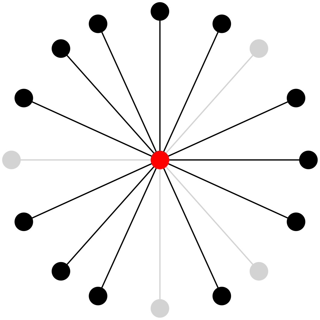
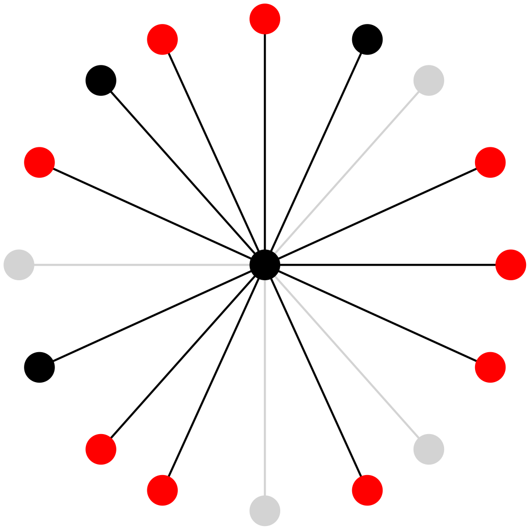
Survival in a star: We consider the star graph induced by a vertex of exceptionally large degree and its neighbours. Furthermore, we assume that the infection rate is small but fixed. By assumption (2.3), at any given time the vertex is on average connected to neighbours via open edges (see (2.4)) and the update speed is of order , for some . Assume for the moment that only the centre is infected, while all neighbours are healthy as visualised in Figure 1(a). Now on average infects
many neighbours before itself recovers or the connecting open edge is updated. Note that is the probability that an infection happens along an edge before updates or recovers.
Hence, after recovery of we are in the situation that roughly neighbours are infected and the centre is healthy, as visualised in Figure 1(b). The probability that all neighbours recover or that their edges update before they could reinfect the centre is approximately
Thus, once an order of many infected neighbours is reached, the total number of infected neighbours will be kept at this order for a time of order where . This implies that if , then the infection persists for an exponentially long time with high probability. This will then be enough time to pass the infection on to the next star.
Transmitting the infection to the next star: Let us assume that the root is initially infected and has a large degree . Furthermore, suppose the centre of the next star that has neighbours is in generation of . Then, the probability that the infection originating from the root is transmitted to in less than time units is approximately
| (3.10) |
for some (see Lemma 7.7 for details). By the previous heuristics we know that an infection can survive in a star of size for a time of order , which means that for a time period of length it is possible for the infection to be transmitted from to without the infection in the star around becoming extinct. Thus, the probability of a successful transmission can be lower bounded by roughly trials of attempting to infect vertex in one go in a time span of length less than . Then the probability that at least one trial is successful is approximately
If the generation is sufficiently small the transmission happens with high probability, i.e. we need that
| (3.11) |
Probability to find another star: In the last step we treat the question, for which offspring distributions it is possible to find a sequence , which grows sufficiently slowly. This boils down to the question how far into the tree do we need to look to find a star of size for a given distribution. Let us first denote by
so that the expected number of stars of size in generation is approximately given by
Now it is easy to see that if
Thus, together with (3.11) we found a lower and upper bound on the sequence , i.e.
| (3.12) |
By this reasoning it follows that if the distribution of satisfies (3.7) with , then we can find a sequence such that with probability bounded away from zero the infection is transmitted to the next star and then back and forth between stars. This can then be used to show that that is reinfected infinitely often for any which implies strong survival in case . This concludes the heuristic explanation of .
On the other hand, if then this argument is no longer true for all . But it can be modified such that we can conclude strong survival if the infection rate is chosen large enough. First, the size of the stars is chosen large but fixed, then by (3.12) if is chosen to be at least of order it still holds true that the infection is transmitted back and forth between stars of size with a sufficiently high probability. This can then be used to show , i.e. strong survival for a sufficiently large as long as .
Remark 3.6.
Our proof strategy is similar to the strategy proposed for the static case by Pemantle [18]. But there are some significant differences. The basic idea for the survival of the infection in a star is that if there is a sufficient number of infected neighbours, in our case , then the infection can persist on its own for a long time. In comparison to the static case we lose roughly many infections in the first steps since additionally to recoveries edges update. Since the star is exceptionally large the edge will be most likely closed after an update. Thus, only many neighbours can be sustained and we lose another for the same reason in the probability of reinfection, which is . In the static case, we would have in both terms instead.
Outline of the article. The remaining paper is structured as follows. In Section 4, we discuss connections to existing results and some open problems. In Section 5, the graphical representation for the contact process is introduced together with the results showing that the critical values do not depend on the particular realisation of an infinite BGW tree. Section 6 is devoted to the proof of Theorem 3.1 and Proposition 3.3. In Section 7, we show Theorem 3.4. The first step of the heuristic, survival in a star, is treated in Subsection 7.2, the second step in Subsection 7.3 and 7.4, and the final step together with the proof of Theorem 3.4 is done in Subsection 7.5.
4 Discussion
In this section we discuss our main results in the context of the CPDG on a BGW tree. We concentrate on our main example, i.e. we assume that the update speed satisfies (2.3) and the connection probability is of the form as defined in (2.5). This means that for every there exists an such that
| (4.1) |
where , and .
Theorem 3.1 and Proposition 3.3 are formulated for deterministic graphs. This means that these two results are applied conditionally on the realisation of the BGW tree . Thus, the specific choice of the offspring distribution does not have an impact on these results. On the other hand, Theorem 3.4 does depend on the choice of the offspring distribution. In the following we discuss the two cases of a power-law and a stretched exponential offspring distribution.
4.1 Discussion for power law offspring distributions
Consider an offspring distribution that follows a power law, i.e. for large with . An immediate consequence of Corollary 3.2, Theorem 3.4 and Proposition 3.5 is the following result.
Corollary 4.1.
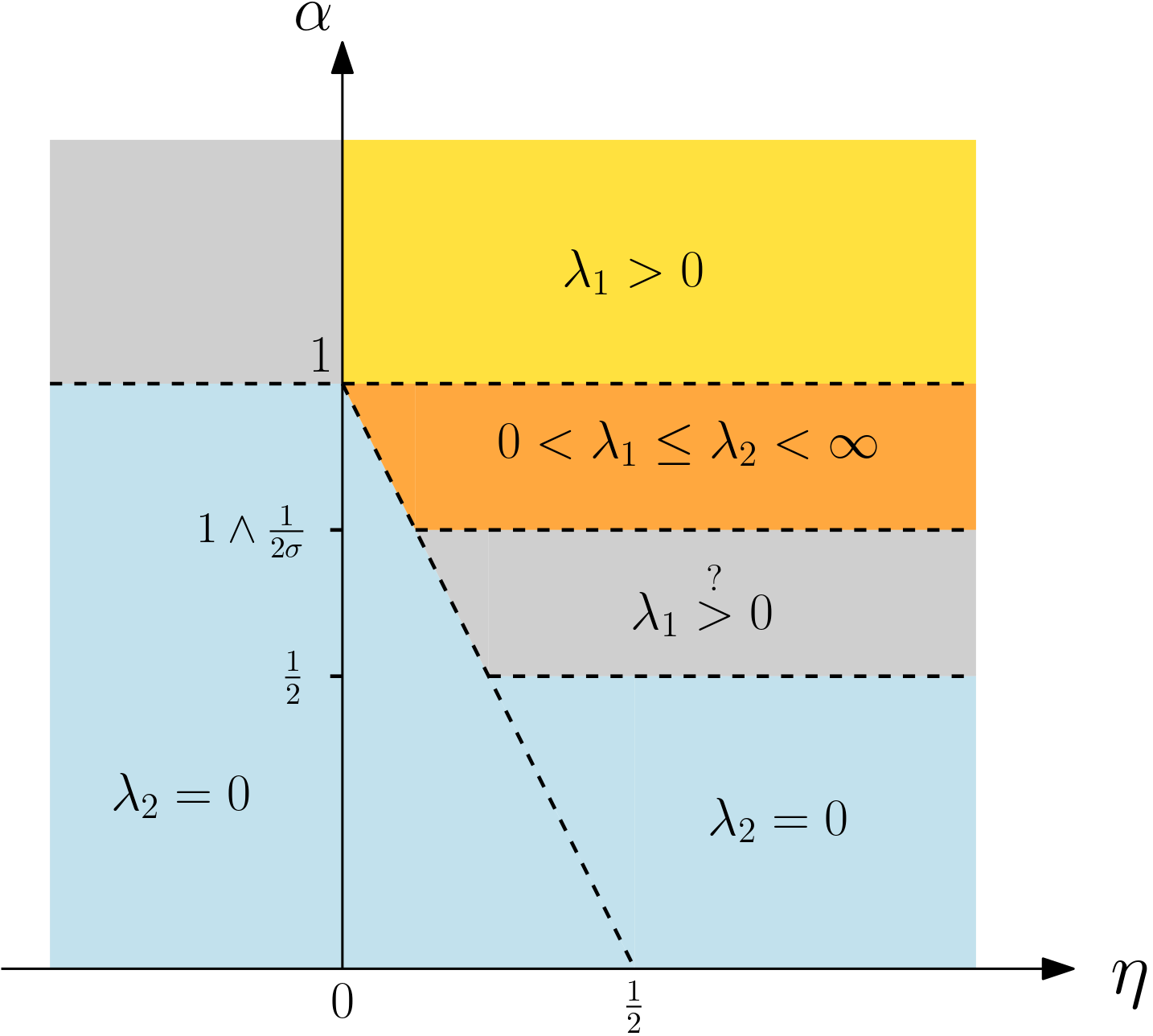
Consider the CPDG on a BGW tree whose offspring distribution follows a power law and has mean larger than . Assume that the connection probability and the update speed satisfy (4.1).
-
(i)
If and either or if and then .
-
(ii)
If either and or if and then .
-
(iii)
If , and then .
Moreover, if then .
We illustrate the resulting phase diagram in Figure 2. A first observation is that the choice of , as well as the offspring tail exponent have no effect on the existence or non-existence of a subritical phase.
Comparison with the static case. At time (and in fact at any given fixed time), the distribution of the number of children of the root is the same as that of
| (4.2) |
Here and are independent copies of the offspring number and conditionally on these the random variables are independent Bernoulli variables with success probabilities , respectively. By calculating the moment-generating function, one can show that has the same distribution as a mixed Binomial distribution , where is an independent copy of .
It is plausible to assume that if we do not allow any updates in the tree, then the contact process on this tree behaves in the same way as the contact process on a static BGW() tree. The difference coming from the correlation of the percolation probabilities of consecutive generations should be negligible. Assuming that and that has a power law distribution with exponent . Then, using a local CLT for binomial random variables and their strong concentration properties, one can show that
where is to be interpreted as upper and lower bounds that agree up to multiplicative constants and we use that the sum concentrates around those values of such that . In particular, has a power law distribution with exponent . The results for the contact process on a static BGW-tree therefore suggest that in the zero update speed case, we always have that for the corresponding critical value . In the case , a standard calculation shows that the percolated offspring distribution has bounded exponential moments, so on a static BGW-tree the contact process has a phase transition.
Indeed, comparing to our model, we have that in the slow speed regime when and , then our model exhibits a phase transition in the same cases as the model on a static BGW()-tree.
However, there is also a major difference between the static and our dynamic model. In the static case, we can choose small enough such that the average degree satisfies . In particular, in that case a BGW()-tree is finite almost surely and the contact process is always sub-critical, i.e. . However, Corollary 4.1 also shows that if , then . Thus, the updating helps the contact process by opening up space so that it can survive for large . Furthermore, for the difference becomes even more apparent since then it holds that . Heuristically one could argue that by letting the model should behave more similarly to the static case, since edge updates become increasingly rare, but this is not reflected in the critical rates. We will come back to this issue below.
Comparison with the penalised contact process. Assume for now that , so that corresponds to a product kernel. As discussed previously, for large update speeds the contact process behaves like the penalised contact process. From the results of [1], we know that in this case, the penalised contact process satisfies if and only if . Under the assumption that , our results fully characterise (with the exception of the case and ) the behaviour of the process. In particular, our model exhibits exactly the same behaviour in the fast speed regime as the penalised contact process when .
In the case , we can thus observe that the dynamical model changes from the static behaviour for to the penalised behaviour for . Moreover, the critical line , interpolates linearly between the two extreme cases.
For general , the situation in the fast speed regime is more complicated and indeed Corollary 4.1 does not fully characterise when there is a phase transition. Nevertheless, we believe that the same critical line as for also characterises the regime between existence and non-existence of a phase transition.
However, it might be that additional moment assumptions on the degree distribution are required. For the special case that the penalisation kernel is given by and for , [1, Theorem 2.5] shows that if (or equivalently that the tail exponent satisfies ), then . However, when , then but . Of course, Proposition 3.3 implies directly that for this special case also in our model holds, but unfortunately we cannot make any statement about . Furthermore,
and thus by coupling the statement of [1, Theorem 2.5(b)] can be extended to for some specific choices of and , but not the whole grey region in Figure 2. However, we believe this restriction to be technical and thus think that in the fast speed regime our model is comparable to the penalised contact process.
Conjecture 1.
Assume the parametrisation (4.1) and and , then if and only if and if and only if .
Immunisation. The second statement of Theorem 3.4 implies that if , then the critical values are finite, , regardless of the other parameter choices. This implies that in this situation no immunisation occurs. (We say that immunisation occurs in a system if for a specific parameter choice .) This is a fundamental difference to the contact process on a dynamical percolation graph considered on in [17] and in the long-range setting in [20, Theorem 2.5] where an immunisation phase takes place. In these models, immunisation occurs if the average degree of the (long-range) percolation graph at every time step is small enough. However, as discussed before, by choosing small, in our setting we can make the average degree at any fixed time arbitrarily small and still have no immunisation phase. One essential difference to the dynamical long-range percolation case is that in the case of we retain the occurrence of vertices with exceptionally large degree. If we know that then the average degree in the thinned tree is . Even though the thinned tree (or rather forest) is fairly sparse or might even only consist of finitely many connected components at any given time point, if we reach a vertex with an exceptionally large degree we can again survive exponentially long in the case that is sufficiently large. This then provides enough time to wait until a connection to another star is established and the infection is transmitted to the next star. On the contrary, if vertices with exceptionally large degree no longer occur. This fact motivates the following conjecture.
Conjecture 2.
Assume the parametrisation (4.1). If then for small enough there exists a such that for all .
Explosion. Finally, we want to comment on the possibility that the CPDG started with finitely many infected vertices explodes in finite time with positive probability. If the offspring distribution has finite mean, i.e. , then the process does not explode in finite time almost surely. This follows by a direct coupling with the classical contact process, where it is know that the process does almost surely not explode if , see e.g. [4, Theorem 3.2] in the case when the fitness is constant equal to one.
On the other hand, if the classical contact process seems to explode in finite time with positive probability. In the case that it appears to us that this can be shown analogously to [1, Theorem 2.5(b)] or more precisely [1, Proposition 6.2]. Note that in that proof it is shown that for the maximum kernel as penalisation when and . This is proved by showing that the infection travels infinitely deep into the tree after a finite time, but it does only return to the root finitely often. Thus, in particular this implies explosion in finite time.
Furthermore, the restriction seems irrelevant for the proof and is in our opinion only in place since is already covered by another result, such that should be possible. For , i.e. but for all , this does not seem to work and it is not clear if the process explodes in finite time.
In this scenario Theorem 3.1 implies for the CPDG that if and , then the probability of explosion in finite time is zero. But in the other parameter regions it is a priori not clear if the process explodes with a positive probability or not.
Again a comparison with the penalised contact process suggests that it is in fact very much possible that explosion occurs for certain parameter choices.
4.2 Discussion of stretched exponential offspring distributions
In the following, we will assume that has stretched exponential tails, i.e. that there exists a such that
| (4.3) |
for some as . Combining Corollary 3.2, Theorem 3.4 and Proposition 3.5, gives the following result for this special case.
Corollary 4.2.
Consider the CPDG on a BGW tree whose offspring distribution has stretched exponential tails such that (4.3) holds for some and has mean larger than . Assume that the connection probability and the update speed satisfy (4.1).
-
(i)
If and either or if and , then .
-
(ii)
If either and or if and , then .
-
(iii)
If , and , then .
Moreover, if , then .
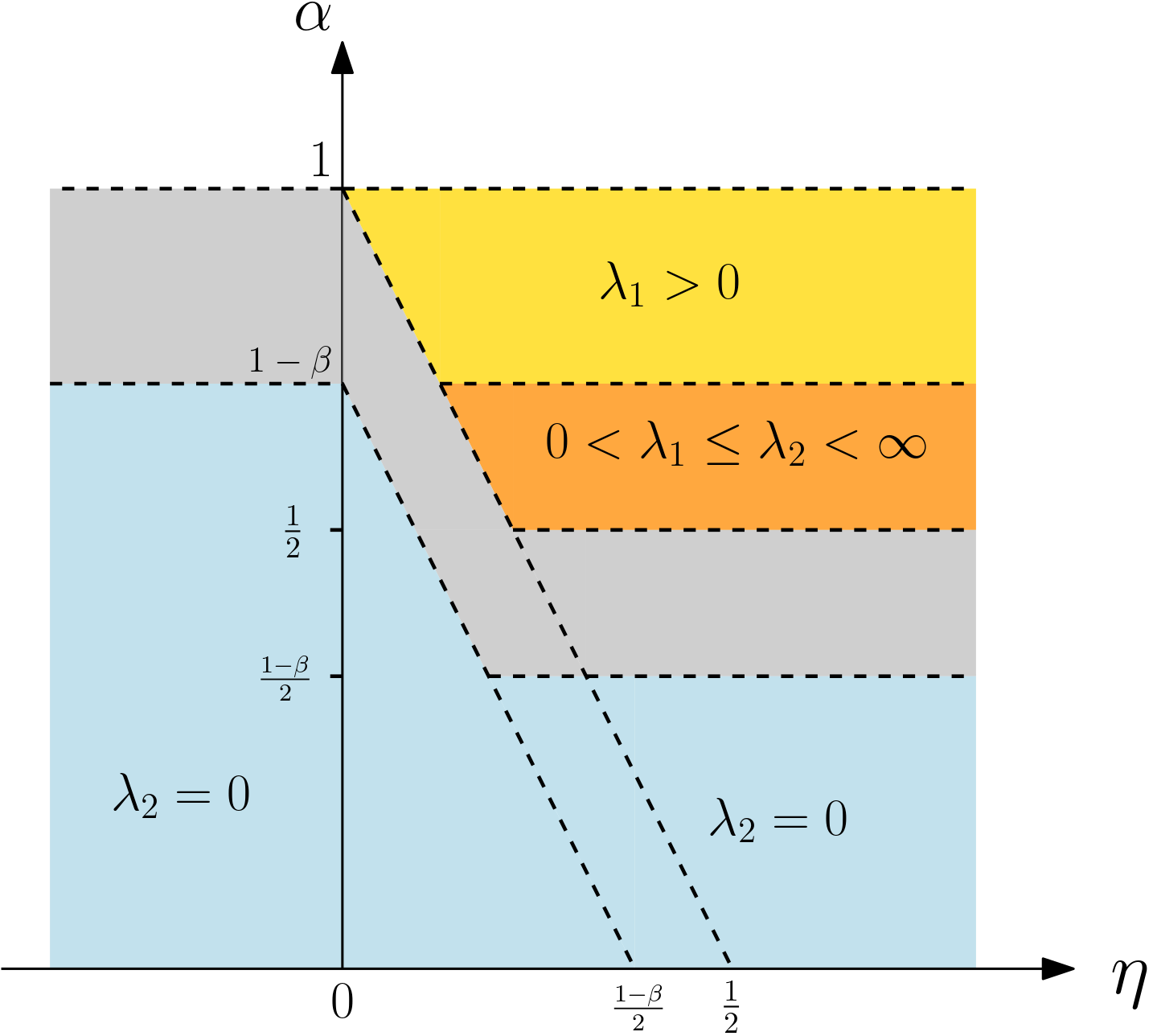
In the case our results do not change, which is not surprising since these results do not depend on the specific graph structure, but only how depends on the degrees. But if , choosing this class of distributions with slightly “lighter” tails compared to the power law distributions has in fact consequences for Theorem 3.4 and Proposition 3.5. In this case we get an additional restriction for our parameter regime, in that needs to be satisfied for (3.7) to hold so that we can deduce from Theorem 3.4. Similary, the condition is necessary so that (3.8) holds and so that Theorem 3.4 yields . We illustrate the additional restrictions in Figure 3 with the product kernel as connection probability.
To see that the additional restriction is natural, it is helpful to again compare to the static case. As discussed before, without updating the model should behave like a contact process on a static BGW)-tree, where is defined in (4.2). However, if satisfies (4.3) and , then does not have any finite exponential moments, so that the static critical parameter satisfies . Moreover, for , the percolated offspring number has some finite exponential moments again, so that the static model exhibits a phase transition. Hence, in the slow updating regime the dynamic model shows the same behaviour as the static case.
For the fast update speed regime, i.e. sufficiently large, the comparison with the penalised contact process yields that for we have . However, for the penalised contact process, as well as for our model, there is a gap in the fast speed case as illustrated by the grey area in Figure 3, where it is not clear whether a phase transition exists or not. Similarly to the case of power-law tails, we would expect a linear transition from the static to the penalised behaviour. However, if we consider the heuristic explanation in Subsection 3.2 and see in the last part that if , then the probability of finding another star of the same size in a reasonable number of steps is not necessarily bounded away from such that the strategy of survival through stars might not work.
This raises the following open problem.
Problem 3.
If we assume that and
does this imply that ?
One possible approach to solve this problem might be to adapt techniques used by [2] to a dynamical setting. With regards to the occurrence of immunisation effects a similar question arises.
Problem 4.
Assume and satisfy (4.1) and that . For small enough, does there exist a such that for all ?
4.3 Comparison with the contact process on finite but large dynamical random graphs
In this final section, we discuss the connections to the models considered in [12, 10, 11]. These study the contact process with either vertex- or edge-updating on inhomogeneous random graphs as the number of vertices tends to infinity. In particular, they give criteria for the existence and non-existence of a phase transition between fast and slow extinction that depend on the exponent governing the update speed as well as the power-law exponent ( in their notation) of the limiting degree distribution of a uniformly chosen vertex. This is in stark contrast to our results, where there is no dependence on the underlying degree exponent (in the power-law case). While the local dynamics of a typical vertex seem similar, these models are difficult to compare. In their model the ‘base graph’ is really the complete graph and the inhomogeneous thinning produces the sparse graph, whereas in our case the underlying tree structure is preserved and we have an additional parameter that controls the thinning.
5 Preliminaries
5.1 Graphical representation
In this section we provide the graphical representation construction for the dynamical contact process on . The general idea is to record the infections and recoveries of the process on on a space-time domain. Let and be two independent families of Poisson point processes. In other words, for every , let and be independent Poisson processes with rates and , respectively. These two processes represent the times at which the edge opens and closes. Furthermore, we define
which is a Poisson process with rate and provides the times of update events on the edge . For every , let us define the following sequence of stopping times
Next let be the initial configuration of the background process , i.e. . For every , we denote by a two state Markov process as follows: we set
for all with . Then we define .
Finally, we define the infection process . Let and be two independent families of Poisson processes such that for all and fixed, the processes and have rate and , respectively. Now we need to introduce the notion of an infection path. Let and with be space-time points. We write if there exists a sequence of times and space points such that as well as and for all with .
Now in order to define the infection process with initial condition we choose a background process with and set as well as
| (5.1) |
The process we just defined has the same transition probabilities as in (2.1) and (2.2).
By now, it is a well-established approach to define variations of the contact process via a graphical representation. If one considers graphs with certain properties, for example finite graphs or infinite graphs with uniformly bounded degrees, it follows by standard results that the constructed process is a Feller process, see for example [15] or [21]. However, in the more general case, where we only assume that the graph is connected and locally finite it is not clear that the resulting process is Feller.
Since in our setting, we cannot ensure that is itself a Feller process, one option is to consider an approximating sequences of processes defined on a sequence of finite subgraphs of by restricting the graphical representation to . To ensure that this sequence of processes, which are then Feller processes, indeed approximates we needed to explicitly assume that we only allow infection paths of finite length in the definition of our CPDG. In fact, this is not a real restriction if the infection process does not explode in finite time. For more details on this see the discussion in Section 6 right before Proposition 6.3.
Remark 5.1.
One advantage of the graphical construction is that it provides a joint coupling of the processes with different infection rules or different initial states. The CPDG is monotone increasing with respect to the initial conditions, i.e.
where and are CPDG. Further, the process is also monotone increasing with respect to the infection rate .
5.2 Properties of on
Let BGW() and recall that we denote by the law of the CPDG on the tree .
Lemma 5.2.
The critical values and are constant -almost surely conditioned on . In particular it holds that
on the event .
The proof follows similar ideas as those used first in [18, Proposition 3.1] and afterwards in [8, Proposition 1].
Proof.
First we deal with the case of . Denote by the survival probability in a given BGW tree with the root initially infected, i.e.
where we are using the notation . We shall prove that
| (5.2) |
which implies that
because if then , and so . Now, assume that the root has children, namely . Then the subtrees rooted in these children are independent identically distributed BGW trees with again offspring distribution , which we denote by . From Lemma 7.6 below, we know that the probability to push the infection from to some conditioned on is given by
Note that by monotonicity
It follows that if for some , then . In other words, if the contact process dies out on then it has to die out on all subtrees . Denote by the generating function of the random variable . Now we observe that
where in the second equality we have used that the subtrees are independent and identically distributed as . This means that
But we know that is a convex function on with at most two solutions of on , namely and If then by convexity for we have iff That means that either or Further, note that as mentioned previously we have
which shows the claim (5.2). This proves that is constant on the event .
Let us now see the proof for . Denote by
Appealing to the same arguments as in the first part, it is enough to prove that if for some , then , since we would get the inequality
by an analogous procedure and therefore the claim follows. Let . Note that for such that , we have
where in the last inequality we have used monotonicity.
Now using again monotonicity of the contact processes, we get
and
where the first inequality holds since switching from to makes the probability smaller since we are considering fewer neighbors. It follows that
| (5.3) |
In addition, we observe that
where the first factor is the probability that the edge is open, the second is the probability that the edge is not updated until time , the third is the probability that infects before time , and the last one is the probability that the infection at remains until time . We observe that we have the same lower bound for since the kernel and the speed function are symmetric. Then, putting everything together in (5.3) and taking yields
In other words, we have deduced that
Since for , we have , it follows that if for some , then . This proves that is constant on the event . For the last claim we remark that it holds that
Since and are constant on it follows that
Thus, we can conclude that on the event it holds that and . ∎
6 Proofs in the general graph setting
In this section we prove Theorem 3.1, Corollary 3.3, and Propositions 3.3 and 3.5. In order to show Theorem 3.1, we will adapt the technique used in the proof of [11, Theorem 5]. Note that [11] always work on finite graphs while we are dealing with an infinite graph. Thus, we need to adjust the proof by using an approximation argument via finite subgraphs. Let be a process with values in , where we again call a vertex infected or healthy if or respectively . Furthermore we call an edge revealed if and otherwise unrevealed.
-
(i)
If an infected vertex shares an unrevealed edge with a vertex then the edge is revealed at rate and is infected if it was previously uninfected.
-
(ii)
If an infected vertex shares a revealed edge with an uninfected vertex then infects at rate
-
(iii)
If is revealed it becomes unrevealed at rate
-
(iv)
Any infected vertex recovers at rate .
We have the following coupling result that is taken from the proof of [11, Theorem 5] but has its roots in [12, Proposition 6.1] and [17]. Since the coupled process is an upper bound it can be used to show extinction for the coupled contact process.
Lemma 6.1.
Let and . Then there exists a coupling such that for all . In particular, if there exists a such that this implies that .
Proof.
We will define a process that is coupled to the processes via the graphical representation using the same Poisson point processes , , and , and then show that the process has the correct dynamics. The evolution of works in the same way as that of , the only difference being that a potential infection event can be used for infection if is a revealed edge even if (so the edge is not open). Recovery events in are used by and in the same way. We will reveal the edge at any potential infection event for which and either or . In this case the infection is also passed on along this edge at time for the process (since then ). An edge will be unrevealed whenever it is updated, so at times .
From this construction, it is clear that we have since the initial states are identical and all infection paths that are used by the process can also be used by . For this note that at any time an edge that is unrevealed but open at will be revealed at time whenever it is used by an infection path for and can then, as a revealed edge, also be used by an infection path for . Also, revealed edges (whether open or closed) can at any be used by an infection path for . Lastly, both processes use the same recovery events.
Thus, it just remains to verify that the process we defined has the dynamics that was described in (i) to (iv) before the statement of Lemma 6.1. The points (ii)-(iv) follow immediately: For (ii) we simply observe that the rate is a consequence of the fact that is for every edge constructed from a Poisson process at rate . Likewise, (iii) follows since update events in for any edge coincide with unrevealment events and happen at rate . Finally, recoveries use , which comes from a rate 1 Poisson process at every vertex, and this implies (iv).
Only the rate claimed in (i) takes a bit more deliberation. First, we note that an edge is only unrevealed at a time if the last event that affected prior to was an update event (as opposed to being revealed and used by an infection path). The outcome of this update event, an open edge with probability and a closed edge otherwise, has thus not been relevant for both infection processes and before time . Thus, is a random variable whose value is independent of and independent of other such Bernoulli random variables (defined analogously for unrevealed edges at infection times). Thus, the rate in (i) for revealment (and potential infection) follows from thinning the rate Poisson process with independent Ber() random variables. ∎
Next let us assume that condition (3.1) holds and set for every and ,
In words and are weighted sums of edges around which are contained in the configuration . Note that due to we have We define for every a score
We also define
where is the number of neighbors which share a revealed edge with . Next, for a given function we define
| (6.1) |
In order to be able to apply the generator to the function , we define the following approximating process. For , set with
where is the graph distance between two vertices in . We consider a new process with state space , where we declare all vertices in to be permanently uninfected and all edges in to be permanently non-revealed. For all other vertices and edges we use same graphical construction as in the original process to describe the infection, recovery and revealment events. Now we set where
| (6.2) |
Note that since all edges in are unrevealed, the corresponding edges do not contribute to the sum defining and so the sum is finite.
Our goal is to show that is a supermartingale for every . For this let us denote by Markov semigroup and by the generator corresponding to .
Lemma 6.2.
Proof.
Suppose that the current state of is . We first list all the possible infinitesimal changes of for .
-
1.
Let us first assume that the vertex is infected, i.e. . Then the following changes can occur:
-
(a)
An infection event between and one of its neighbors occurs and the edge was previously unrevealed, i.e. . This would cause a change of . Now summing over the neighbours of yields that the total rate of change is
-
(b)
The cumulative change caused by update events at revealed edges between and its neighbours is
-
(c)
A recovery event at results in the change .
-
(a)
-
2.
Next we consider to be healthy, i.e. .
-
(a)
The cumulative change caused by infection events along unrevealed edges between and its neighbors is
-
(b)
If the infection event between and its neighbors happens at a revealed edge the cumulative change is
-
(c)
The cumulative change of all update events at revealed edges between and its neighbors is
-
(a)
Now by adding up the individual contributions we listed before we get that
(Note that the sum over is only over which are not infected. We can simplify and ignore the negative contributions from in the second and in the very last sum in order to obtain
| (6.3) | ||||
Now the right hand side of (6.3) can be split in four terms. Let us first handle the terms with negative sign. Since for all and so it follows that
| (6.4) | ||||
Finally we deal with the remaining term on the second line of (6.3) and change the order of summation so that we get
where for the inequality we have once again used as well as assumption (3.2) on the function . With this fact and (6.4) we get by plugging back into (6.3) that
Now by adding in some positive terms (involving ), we obtain that
where we have also used that if . ∎
We can now use Markov semigroup theory which yields that and use the bound on the derivative found in Lemma 6.2 to find a suitable bound on . Then we take the limit as to deduce that goes extinct.
For this purpose, we define an approximation process analogously to . We define by restricting the graphical representation introduced in Section 5.1 to the finite subgraph , where we declare all vertices in to be permanently uninfected and all edges in to be permanently closed. By definition it follows that the sequences of (random) sets are monotone in , i.e. for all , which implies existences of the pointwise limit and also that
| (6.5) |
Now we only need to ensure that holds true for all . It is clear , since edge updates happen independently of each other. In the case of the infection process the equality could only fail if there exists an such that . But in the definition of we explicitly assumed that infection paths are of finite length, and thus there must exist an such that , which implies that .
Proposition 6.3.
Let such that and is a finite set. Suppose that condition (3.1) and that (3.2) and (3.3) of Theorem 3.1 hold. Then it follows that
for every infection rate . Assume further that
| (6.6) |
Then it follows that the process defined as in (6.1) is a supermartingale for every , which converges almost surely to as . This implies in particular that goes extinct almost surely.
Proof.
We first consider the processes and By Lemma 6.2 and (3.3) we get for that
Therefore, for sufficiently large such that ,
| (6.7) |
Moreover, since and when , we obtain that . It follows by Markov’s inequality that for any
Further, using Lemma 6.1 with the processes and , we see that these processes can be coupled such that for all and , which together with the previous inequality implies that
But we have that since As for any we have it is clear that the right-hand side is smaller. In order to see the reverse inequality we note that if holds then there exists an such that and we will by the convergence also have that for large enough , and thus .
This implies
| (6.8) |
Now using that that is decreasing in and continuity from below of the probability measures, we get that
Thus, it follows that for all which in turn implies that
For the last statements, we assume that . From (6.7) and Markov’s property it follows that for each the process is a supermaringale such that as almost surely. In addition, by (6.8) and the continuity of probability measures
as . ∎
Now Theorem 3.1 follows as a corollary. We just need to pick a small enough such that (6.6) is satisfied.
Proof of Corollary 3.2.
Assume that and satisfy (2.3) with . Since is decreasing in both parameters and for any , we have
Using the same arguments we also have the corresponding bounds for . In other words, we deduce that
| (6.9) |
With this in hands, we can check conditions (3.2) and (3.3) of Theorem 3.1. We first prove the statement under condition . Therefore, we assume . Then we choose , then it follows that for all
where in the second inequality we used that since . On the other hand, we observe that (6.9) implies that for all
where in the last inequality we used that and . Therefore, the conditions of Theorem 3.1 are satisfied, and thus and the infection process does not explode for any infection rate .
Now we consider the condition . Thus, we assume that the connection probability is of the form as defined in (2.5), where , and , and still satisfies (2.3). Note that it suffices to show the statement for , since is already covered by the first case . Let for some , which is well-defined since . Now, we observe
where in the inequality we used that and that , which follows since . Hence, we see that for any
It follows that for any
where we used that . For condition (3.3), we observe that
where in the last inequality we used that . Therfore, again the conditions of Theorem 3.1 are satisfied, which yields the claim. ∎
Proof of Proposition 3.3.
Let be such that (3.1) holds. Following similar arguments to those used in the proof of Theorem 2.2 in [20] (based on the coupling of [3]), we can couple the process with a contact process such that for all , with an infection rates defined as follows
for all . Note that we explicitly indicate the dependence on since in the second part of the proof we consider . Denote by for the critical values for weak and strong survival of the process on . Then by the coupling we immediately have for . Note that by rearranging the terms we see that
Now, using the inequalities , which hold for all , we deduce that
| (6.10) |
Since we assume in (3.1) that we obtain that
Denote by a penalised contact process with infection rate , i.e. the infection rate along an edge is . Now we can obviously couple to such that for all . In other words, for , where and are the critical values for weak and strong survival of . Now we assume that (resp. ), i.e. the penalised contact process with rates survives weakly (resp. strongly) with positive probability for all . In particular, the process survives weakly for , corresponding to the transition rates of . Then (resp. ). This provides the first claim.
Now we consider a sequence of update speeds. Then by using a Taylor expansion one can show that as , see for details the proof of [20, Lemma 5.9]. It turns out that as for , which can be shown exactly as in the proof of [20, Corollary 2.4] (we point out that condition in [20, Corollary 2.4] is only used to get the uniform control over , but here it follows from (6.10) and the definition of ). This yields the second claim, i.e.
We finish this section with the proof of Proposition 3.5.
Proof of Proposition 3.5.
In this proof we denote by the critical infection rate for local survival for the penalised contact process on the BGW tree with transitions as in (3.4) and with penalisation chosen to be as in (2.5) with , and such that (3.9) holds. Note that for , and by [1, Theorem 2.1] it follows that . Now if , then , and thus it follows directly that . Furthermore, we see that for all , and this is also true if we replace in with such that . Therefore, by monotonicity of the penalised contact process in the infection rates it follows that This implies for all and . Finally, the claim that the critical infection rates of the CPDG with connection probability equal , i.e. follows by Proposition 3.3. ∎
7 Proofs in the tree setting
The goal of this section is to prove Theorem 3.4. As described in Subsection 3.2, the proof strategy relies on two key arguments. The first argument is that the infection can survive in the neighbourhood of a vertex of exceptionally high degree for a time of exponential order. We call such vertices stars. The second argument is that we will consider relatively heavy-tailed offspring distributions, allowing the infection to reach the next star of at least size fairly quickly. We present the technical auxiliary results in the subsequent Subsections 7.1-7.4 in detail. Finally, in Subsection 7.5, we bring them all together to prove Theorem 3.4.
Throughout this section, in most cases, we consider the root to be a star. Thus, for the sake of readability we introduce some notation. If we condition on , where will be chosen to be sufficiently large, we write (resp. ) instead of (resp. ).
For the rest of this section, we fix an such that , where is a given offspring distribution with . The condition ensures that if we prune the random tree by only keeping vertices of degree less than from generation onward, then this random tree is still supercritical.
Due to Condition (2.3), for given and , we find constants which only depend on such that
| (7.1) |
for . Throughout this section, we assume that .
7.1 Stars and stable stars
We will first focus on the first argument, which is to understand how long the infection can survive restricted to the neighbourhood of a star with sufficiently high probability. The results in the next two subsections are very similar to what is discussed in [11, Section 3.3]. Thus, we will omit some of the proofs, which can be proved analogously.
Since we consider a dynamical tree we need to find a space-time structure which can keep an infection alive for a time of exponential order. For technical reasons we need to only consider neighbours of which are of bounded degree. We denote by
the set of all offspring of with degree less than or equal to . Next we define
Note that for and the overlap of consecutive intervals is of length . Recall that and are the Poisson point processes describing the recovery times of and the updating times of the edge , respectively. Now we define the set of good neighbours of in the interval as follows
In words a good neighbour in is a neighbouring vertex of which itself has degree less than or equal to and is connected to at time . Additionally, the edge is not updated within , and therefore is connected to for the whole time interval . Furthermore, does not recover which implies that if is infected, it will remain infected until at least .
As described in Subsection 3.2, a star can be thought of as reservoir for the infection, where it can survive for an exceptionally long time without input from outside. Furthermore, during this period we want to push the infection to the next star. Thus, for technical reasons it is more convenient if the path towards the next star and the reservoir are defined on disjoint parts of the graph, except for . Thus, we need to be able to exclude a given vertex from the set of good neighbours. Therefore, we define for every the set
In the next result we show that with high probability we have enough good neighbours around the root for a sufficiently long time. This lemma can be proved analogously to [11, Proposition 3]. We will nevertheless give the whole proof for two reasons. First we adapted the statement slightly and secondly since we consider a different model compared to [11] there are minor differences in the proof, and thus we would like to highlight this once.
Lemma 7.1.
There exists independent of and such that for large enough
Proof.
As is fixed, we write for throughout. Note that for the random variable has a Poisson distribution with mean bounded by , where we used that we conditioned on , (7.1) and that by definition . Now, by definition of the set and being a decreasing function, we have for every with that
where we also used that we condition on . Thus, we get that
where , and we recall that is the number of offspring of vertex and by (3.5) we have . Since the number of offspring are sampled independently for every parent in a BGW tree, this implies that stochastically dominates a binomial random variable . By the Chernoff bound for a binomial distribution (see e.g. Theorem 2.21 in [7]), we get for that
| (7.2) |
Next set and observe that
| (7.3) | ||||
Thus, by using the fact that stochastically dominates and (7.2) we get that
Note that if , and thus if we choose and set we have
Now for large enough it holds that , and thus we have by plugging back into (7.3)
which yields the claim. ∎
We say that is a stable star if the following event holds
| (7.4) |
Since we only consider stable stars in the subsequent subsection we mostly refer to just as a star. Note that Lemma 7.1 tells us that for large enough
Furthermore, in most cases we need to exclude a specific neighbour , and therefore we define the event
| (7.5) |
The reason for excluding a specific neighbour is to ensure that the previously mentioned reservoir around and the path towards the next star only share the centre and otherwise are defined on disjoint parts of the graph. Note that acts as a lower bound since for all .
7.2 Survival on a star
In this section we study survival of the contact process on a (stable) star and for notational convenience formulate the results for being a star. So let us introduce the process defined via the same graphical representation as but restricted to , i.e.
-
1.
we set to be the initial configuration and
-
2.
an infection event at time is only valid if .
This means that only and its good neighbours can participate in infection events. Now we define the set of good infected neighbours of as follows
| (7.6) |
where some is excluded. In words this is the set of good neighbours in the interval , which are infected at time , and thus are infected at any time during since good neighbours do not recover during . Furthermore, we denote for any and by the -algebra generated by the graphical construction up to time , and the processes and for all up to time .
Note that in all results in the subsequent subsection we are only concerned with the number of good infected neighbours rather than which neighbours specifically are of this type or which neighbour exactly was excluded. Therefore, for the sake of readability, we omit the argument , and write , , , and , as long as it is clear from the context.
In the next step we need to know how long the centre of a star is typically infected if we already have “enough” infected good neighbours. The following lemma states that the centre of a star with enough infected good neighbours will be infected for at least half of the time within a time interval with high probability.
Lemma 7.2.
Let . There exists a constant independent of , such that for any with and any we have
Proof.
The claim can be proved analogously as [11, Lemma 2]. ∎
The next lemma shows that with high probability the infection will persist for a long time in a stable star if we already have a sufficient number of infected good neighbours. Before we start we introduce some notation, set and define the following event
where . Here again we drop the dependence on and only write , as long as it is clear by context. Note again that the subsequent result is independent of the specific choice of .
Lemma 7.3.
(Local survival) Let and be chosen such that and set . Then there exists a large universal constant such that if for any , we have
on the event .
Proof.
The result follows analogously to [11, Proposition 4]. ∎
With this result we have control over the event that an infection persists for an exponential time if we already have a sufficiently large pool of infected good neighbours which can sustains the centre to be infected most of the time. It remains to estimate the probability to reach this amount of good infected neighbours in case that only the centre is initially infected.
Lemma 7.4.
Let and be chosen such that . Furthermore, let and . Then it holds that
on the event .
Proof.
By the choice of we see that , and thus the probability that does not recover in is bounded from below by . On the other hand, the probability that an infection event happens between a good neighbour and in the time interval is bound from below by . Note that the last inequality holds since . Now given that does not recover in we concluded that on the event the random variable is stochastically dominated by a binomial random variable with trials and success probability . Recall that , where is the constant from Lemma 7.1. Therefore, we get that
Next we can again use a Chernoff bound for the binomial distribution (see e.g. [7, Theorem 2.21]) to obtain
where in the last two inequalities we have used and for , respectively. Thus, it follows that
as claimed. ∎
7.3 Pushing the infection along a path
Given a single path of length on the vertices such that for , the goal in this subsection is to find a lower bound on the probability where we let . We begin by finding the probability to pass the infection along a single edge. In order to do so, we first make the following simple observation.
Lemma 7.5.
Let be independent exponential random variables with parameter and let be independent exponential random variables with parameter . Let be independent of everything else, then
has the Laplace transform
| (7.7) |
Moreover, has the same distribution as the sum of two exponential random variables with parameters
Proof.
We calculate for ,
For the second claim, we recall that the Laplace transform of the sum of two independent exponential random variables with parameter and has the form
By comparing factors, we see that and have to satisfy
which is true by taking and as in the statement of the lemma. ∎
For the next lemma we consider some arbitrary but fixed edge . We denote by and the first true infection time on and the first recovery time of , i.e.
Lemma 7.6.
It holds that
| (7.8) |
Furthermore, for any
where
| (7.9) | ||||
Proof.
For simplicity we drop the argument and write and . Suppose that initially the edge is closed and we denote by referring to . Set and for , iteratively define
as the times at which an edge opens and then the times, once the edge is open, for the edge to either close or for an infection to be passed along. Denote the corresponding waiting times as
Now, define
as the indicator for the event that on the -th trial an infection event takes place rather than a closing event.
By the properties of Poisson processes and their exponential waiting times, the random variables , are all independent. Moreover,
| (7.10) |
Then, if we define to count the total number of trials to pass the infection along the edge, we have that is a geometric random variable with parameter that is independent of . Thus the first time when we have a true infection can be written in terms of these waiting times as follows,
| (7.11) |
Denote by the density of . We can now calculate by independence and then Fubini’s theorem the following probability
Using the representation in (7.11) and Lemma 7.5 with and we get the first claim. For the second claim, we first see that
| (7.12) |
By the second part of Lemma 7.5 we know that has the same law as the sum of two exponential random variables and with parameters and as defined in (7.9). Then it is straightforward to see that
which yields
Plugging this back into (7.12), we get
Using (7.8) together with the identities and , we deduce the desired result. ∎
Finally we will show a lower bound for the probability of pushing the infection along a path of bounded degree to a stable star. The proof uses a similar line of arguments as in [4, Lemma 5.1], however the presence of the dynamical graph structure leads to some changes. In order to do so, we first introduce some notation.
Let and denote by the set of vertices in generation . Note that due to the tree structure of we find a unique path from to , which means that for every .
For any vertex , we define the subgraph where the vertex set is given through and we consider all edges such that . Now we introduce the process , which is defined via the same graphical representation as but the infection is restricted to , i.e.
-
1.
we set to be the initial configuration and
-
2.
only infection events contained in the subgraph are used.
This means that only vertices contained in participate in infection events, and therefore, as long as it follows that for all .
Now we define as the set of all vertices in generation with degree which are connected to via a path consiting of vertices with degree bounded by , i.e.
| (7.13) |
We emphasize here that the notation in what follows corresponds to the conditional probability on the tree and on the event that the root is infected and the background process starts in any distribution.
Lemma 7.7.
Let . Suppose the background process is started in an arbitrary distribution. Let and is the unique path from to then there exists a constant independent of such that
Moreover, let with and suppose that and satisfy (2.3). Then for it follows that
where
| (7.14) |
Proof.
Let us consider the true infection point process on the edge . By this we mean only the times such that , which we denote by
Let us define the sequence of random times as and for set
Furthermore, define with for . Also denote by
where is the event that infects before it recovers. Now we see that
| (7.15) |
Recall that from Lemma 7.6, we have
By monotonicity with respect to the initial condition in the background process, we have
which implies due to the Markov property that
| (7.16) |
On the other hand, appealing to Markov’s inequality and the definition of and , we have, for any
where in the second inequality we have used that the waiting time is larger when we start with closed edges and in the third inequality we have used that is independent of for all and also the times are independent of each other.
Now appealing to Lemma 7.6, we have that
where and are defined as in (7.9) for the corresponding edge . This is the distribution of the sum of two independent exponential random variables with parameters and . Since , by a coupling argument one can show that the law of the sum of two standard exponential random variables stochastically dominates the law of . We also know that the distribution of the sum of two standard exponential random variables is a Gamma distribution with parameter and . Then the law of is stochastically dominated by the law of where , which implies
where . Now, note that
Therefore, by choosing small enough, we can deduce that there exists such that
| (7.17) |
Plugging (7.3) and (7.17) back into (7.15), we get the first statement. For the second claim, we assume that the update speed and satisfy (2.3), and that . First, we deal with the case . Since for all in this case we have , which yields
Furthermore using that , we get that
Therefore, using the first statement of the lemma together with the inequality which holds for and the fact that is decreasing in both arguments, we get that
For the case we have that for all and , and furthermore that for all . Now using that is a monotone function we get that
for all and for it follows that
Since is a positive decreasing function in both arguments, we deduce that
Furthermore, we know that for , and thus we get that for all that
This concludes the proof. ∎
7.4 Transmitting the infection from one star to another
In this section, we finally want to bring together the main results of the previous two subsections. We will now define an infection process , which is restricted to the neighbourhood of the root and a single path leading to a star in generation .
For any vertex we define the subgraph , where the vertex set is given through and we consider all edges such that . Now we introduce the process , which is defined via the same graphical representation as but the infection is restricted to , i.e.
-
1.
we set to be the initial configuration and
-
2.
only infection events contained in the subgraph are used.
This means that only vertices contained in participate in infection events, and therefore, as long as it follows that for all .
If we start with only the centre of a star infected, we estimate the probability to push the infection to the next star. We use Lemmas 7.3 and 7.7 to find a lower bound for the probability that the star , which is at distance from the root and has the same degree as the root, is infected before the infection dies out around the root.
Before we proceed, we recall some notation. We defined the set of good infected neighbours by in (7.6), where a given is excluded. Similar we defined the the -algebra to be generated by the graphical construction up to time , and the processes and for all up to time . Note that for the sake of readability we omit , whenever it is clear from the context. Lastly at the beginning of Subsection 7.2 we defined .
The next lemma shows that, if the root has enough good infected neighbours then the root is infected with sufficiently high probability at a given time.
Lemma 7.8.
Let and with . Now set , then it holds that
on the event .
Proof.
Let us first consider a simpler setting, that is we consider a star graph with centre and leaves denoted by . We consider the following situation: we start with every leaf infected and the root healthy. Furthermore, the leaves are unable to recover, but the root can. We want to find a lower bound on the probability that the root is infected at time . This problem is described by a two-state Markov process on the state space , where is either infected (state 1) or healthy (state 0) and we use the Poisson processes and to construct it. Set
We set initially . Now at any time point in the process jumps to state and at any time point in it jumps into state , i.e. we get a Markov process with transitions
The distribution of this two-state Markov process is well-known,
(see e.g. [16, Example 2.6]). Using the inequality which holds for all , we see that
and thus
Now we come back to our original goal. Since we are on the event we know that there exist at least good neighbours which are infected. By the definition of good neighbours we know that they do not recover and they are connected to the root until time . But this means we are again in the same setting as above, since we have a star graph with at least infected leaves which are unable to recover and we want to know what the probability is that the root is infected after a time step of length . Hence, by monotonicity we get the claim. ∎
The next lemma provides an upper bound for the probability that the number of infected good neighbours during the time interval is at most given that the root is initially infected and has degree , where as defined in Lemma 7.3 for with chosen as in Lemma 7.1. Finally, recall that with is the event that is a stable star, where is excluded, defined in (7.5).
Lemma 7.9.
Let , and be chosen such that and , where denotes the universal constant given in Lemma 7.3. Suppose the background process is started in stationarity. Then, for large enough it holds that
on the event , where
| (7.18) |
and
| (7.19) |
Proof.
In the whole proof we exclude from the star. Thus, we suppress it in the notation and only write , and . We begin by observing
Now note that the conditional probability of on is the same as on , since only depends on events in the graphical representation contained in the time interval . Therefore, it is independent of everything happening after the time point . By Lemma 7.3, we deduce that the inequality
holds on the event and with Lemma 7.4 it follows that
holds on the event . In summary we get that
holds on the event , which proves the claim. ∎
The next lemma gives a lower bound for the probability that a vertex in a given generation is infected if we start with the root infected and condition on the event that the root and such vertices have the same degree. For the next result recall the definition of and from (7.14).
Lemma 7.10.
Proof.
For the sake of readability we will again omit if possible the subscripts and the argument and write , and throughout. The function
is monotone decreasing, and therefore it suffices to derive the bound for . Let and set . Recall that we denote the unique path from to by . We begin by noting that
| (7.22) | ||||
Thanks to Lemma 7.9 we know that the first probability on the right-hand side is bounded from above by on the event .
Thus it is enough to derive the upper bound for the second probability. Define the sequence of times such that and for . Now set for , then we see that
Now set
Note that by definition it holds that . The tower property implies that
where we used that by definition of we have and also that . Now, define the following two events
with , then we see that . Therefore,
where we used the tower property, since , and that by definition. Recall that before Lemma 7.7 we defined the infection process , which is restricted to the path from to . By definition it follows that for all . Let us empasize at this point that by excluding from the set of good neighbours the path leading from to and the set are defined on disjoint parts of the graphical representation for all . This enables us to use the Markov property and monotonicity to obtain that
where we have used that . Thus, we obtain that
Moreover, appealing to Lemmas 7.7 and 7.8 we get
and
These two inequalities now yield that
Now we can recursively conclude
where in the last step we treated the first time interval differently, since we know that at time the root is infected, and thus we do not need to reinfect it in the first time period. Recalling that we chose , we can conclude
and thus the claim is proved. ∎
7.5 Proof of Theorem 3.4
The aim of this section is to combine the results of the previous sections and show the two statements of Theorem 3.4. Throughout the section we suppose that is a CPDG with initially infected and that the background process is started stationary. Let be a fixed constant large enough such that
| (7.23) |
We recall that the first claim of Theorem 3.4 is that if , and (3.7) holds then . In other words, for every local survival takes place with positive probability. The second statement is that if and (3.8) holds then , i.e. for large enough local survival takes place with positive probability. Note that it is sufficient to consider in order to show this claim because the case is covered by the first claim. Therefore, we need to consider two parameter regimes. First let
| (R) |
where is the universal constant given in Lemma 7.3. Note that if we show the first statement for it follows by monotonicity for all . The second parameter regime is the following
| (R’) |
Observe that in both cases we have that for all large enough, which is necessary for several results in the previous sections.
We recall from Section 3.2 that our strategy is to apply [18, Lemma 6.2] to the function
In order to do so, we need to find a non-decreasing function on such that in a neighbourhood of and show that and satisfy
| (7.24) |
where is chosen as in (7.18). For simplicity of exposition, we split the proof of Theorem 3.4 into several lemmas. The first lemma gives us a good candidate for the function .
Lemma 7.11.
Proof.
Let and be the unique path from to and also let
Recall that the process is defined via the same graphical representation as but the infection is restricted to . We begin by noting that due to the monotonicity of the CPDG, we have
Now, Lemma 7.10 tells us that
on the event , where is defined as in Lemma 7.9, the functions and are defined in (7.19) and (7.20), respectively. Then, using the inequality , observe that ( ‣ 7.11) forces to be at most , i.e.
Furthermore, the asymptotic result derived in Lemma 7.4 implies that if , if and if , as . Hence, there exists an sufficiently large such that for all . Thus, it follows that
| (7.25) |
Before we proceed we need to introduce some further notation. Given a realisation of the underlying tree we denote, analogously to (7.5), by the event that is a stable star starting from time , where . Furthermore, we explicitly exclude the neighbour in generation , but we do omit this in the notation to avoid clutter. In the following, we will condition on the event
i.e. that for some which is a stable star starting at time . We deduce for
where
Hence, the next goal is to establish lower bounds for the functions and .
Lower bound for . Recall that we denote by a generic random variable distributed according to the offspring distribution of . Note that the expected number of vertices in can be bounded from below as follows
| (7.26) |
where we used symmetry and monotonicity. Let be the number of vertices in infected before time , that is
Then, by using the fact that for all , followed by the tower property and (7.25), we deduce
Now we observe that from (7.26), we get
where we used that as was pointed out at the end of Section 7.1. In addition, by Lemma 7.1 we have that . Thus there exists such that for large enough . In other words, we deduce
Let us define, for ,
Now, ignore all the infections of by its parent except the first infection. Then, the contact process on the subtrees rooted at vertices which are infected at some time will evolve independently from time to time , since by the branching property of the BGW tree and using that the background process is stationary. Then the vertex will be infected at time with probability at least .
Furthermore, the event that is a stable star from onwards, i.e. that is satisfied, is independent of everything that happened before time and by symmetry it follows that is a lower bound for the probability of being a stable star for every realisation , i.e. .
If we denote by the random number of vertices in which are infected at time and are stable stars starting at , we can conclude that stochastically dominates a random variable that has distribution . Appealing to Lemma 2.3 in [18], there exists such that
Moreover, since dominates the random variable , we obtain that, for
| (7.27) |
which implies for
| (7.28) |
Lower bound for . Let . Note that
where
Now, we need to find lower bounds for and .
For that purpose we need to introduce a bit more notation. Let be the -algebra which is generated by the graphical construction up to time . Furthermore, we denote by the -algebra generated by and for all , i.e. vertices in generation , and with , i.e. edges between generation and . In words this means that contains all the information about recoveries in generation and update events between generation and for the whole time period to . Finally we define the -algebra for .
We begin with the lower bound for , where we get by the tower property that
Recall that on the event we know that there exists an which is a stable star from onwards and , i.e. is infected at time . This means we are again in a situation that we can consider the restriction of the graphical representation to a path of length between and the neighbourhood of . Then, it follows analogously as in the proof of Lemma 7.10 and (7.25) that
where we used that the path is between generation and , and thus independent of everything in generation and higher. Therefore, we can conclude that .
Next we derive a lower bound for . Let us now introduce the stopping time for the contact process ,
The aim is to deduce a lower bound for the probability of the root being infected at time . Thus, we can use monotonicity to restart the infection process after time with only being infected. Furthermore, after we restrict infections to and its neighbourhood, i.e. we restrict the graphical representation to from onwards, analogously as in the definition of . We denote
Note that on we have at least good neighbours in . Further, define to be the event that at least one of the neighbours which are infected at time infects at a time in before this neighbour recovers and
With this notation we can estimate as follows,
| (7.29) |
where we used that the event is independent of , since these events are defined on disjoint parts of the graphical representation. On the other hand, recall that we denote by the -algebra, which is generated by the graphical construction up to time . Thus, using that and the independence of the infection and recovery events, we obtain
Now we find a lower bound for the two conditional probabilities on the right-hand side of the previous equality. First note that . Recall that are the neighbours of with degree less than , i.e. for all . Denote and by the neighbours that are infected at time . Note that we can rewrite the event as follows
Further,
Thus,
where we used that only depends on the graphical representation in the time interval .
On the other hand, by monotonicity we get
where
Now, appealing to the strong Markov property and Lemma 7.9, we deduce that
Putting everything together yields
Hence, substituting back into (7.29) we deduce
Note that as for all . Further, we recall that if , if and if , as . Thus, we find a and a constant such that for we have for all . Finally, the lower bounds for and give that for
This yields that, for ,
where . Under the assumption that satisfies Condition ( ‣ 7.11), we have established the following lower bound for ,
This together with the fact
implies that there exists such that
and the desired result follows. ∎
The following lemma tells us that under the Condition (3.7) we can find a natural number such that Condition ( ‣ 7.11) holds for large enough.
Lemma 7.12.
Proof.
By Assumption (3.7), we have that there exists a subsequence such that as and
| (7.31) |
For the rest of this proof we write and . Note that for this sequence it also holds that as , which implies that as .
The proof is completed as soon as we can show that Assumption (3.7) implies for sufficiently large that the following inequality holds
| (7.32) |
where we can avoid the ceiling and the floor in the factors and as as (and similarly for and ). Therefore, (7.32) is equivalent to ( ‣ 7.11) for large enough. Now, we see that (7.32) is equivalent to
| (7.33) |
Further, we observe that
| (7.34) |
where in the first limit we have used that for all and as . For the second limit we have used that there exist such that
| (7.35) |
which follows for large enough by (2.3) and (R). This yields that
Therefore, when is large enough (7.33) is implied by
| (7.36) |
Furthermore, recall from (7.14), then we see that for large enough this is equivalent to
| (7.37) |
Now, we will see that (7.31) implies (7.37). Suppose that is sufficiently large so that
| (7.38) |
Since , and by (7.35), we can assume that is sufficiently large so that
Moreover, by (7.31), we have
Then we can choose large enough such that
In other words, we have for this choice of that
where the last inequality is implied by the choice of in (7.38). Therefore, (7.37) holds, which concludes the proof. ∎
Lemma 7.13.
Proof.
Similar as in the proof of the previous lemma by Assumption (3.8), we have that there exists a subsequence such that as and
| (7.39) |
Again we write the rest of this proof , and . It follows that for this sequence it holds that as , which implies that as .
We have to show that Assumption (3.8) implies for sufficiently large that the following inequality holds
| (7.40) |
Similarly as in Lemma 7.12, we deduce that
Thus, when is large enough (7.40) is implied by
Note that the right-hand side does not depend on . Since , we require for this equality to hold that
| (7.41) |
We point out here that we are assuming that , and thus . Now the fact
guarantees together with (7.39) that (7.41) holds for large enough since the limit diverges. In other words, defined as in (7.30) satisfies Condition ( ‣ 7.11) for some large . ∎
We are now ready to deduce Theorem 3.4.
Proof of Theorem 3.4.
Let us begin with the first claim. Assume that Condition (3.7) holds, and . Fix . Next define as in (7.30). By Lemma 7.12, we know satisfies Condition ( ‣ 7.11) for some large enough. Now, we are able to apply Lemma 7.11 to deduce that the non-negative and non-decreasing function
satisfies
where . Furthermore, we observe that
In addition, by definition of , we have , which implies in a neighborhood of 0. Thus appealing to Lemma 3.4 in [18], we conclude that
and thus
which in turn implies that .
For the second part, we fix and and assume that Condition (3.8) holds. Now, for , we choose and as in (7.30). By Lemma 7.13, we know that for some large the term satisfies Condition ( ‣ 7.11). Therefore, using the same arguments as before we can conclude that for this choice of the infection rate,
which allows us to conclude that . ∎
Acknowledgement. MS was supported by the LOEWE programme of the state of Hessen (CMMS) in the course of this project.
References
- [1] Z. Bartha, J. Komjáthy, and D. Valesin. Degree-penalized contact processes. Preprint, arXiv:2310.07040, 2023.
- [2] S. Bhamidi, D. Nam, O. Nguyen, and A. Sly. Survival and extinction of epidemics on random graphs with general degree. Ann. Probab., 49(1):244–286, 2021.
- [3] E. I. Broman. Stochastic domination for a hidden Markov chain with applications to the contact process in a randomly evolving environment. Ann. Probab., 35(6):2263–2293, 2007.
- [4] N. Cardona-Tobón and M. Ortgiese. The contact process with fitness on random trees. Preprint arXiv:2110.14537, 2021.
- [5] S. Chatterjee and R. Durrett. Contact processes on random graphs with power law degree distributions have critical value 0. Ann. Probab., 37(6):2332–2356, 2009.
- [6] T. E. Harris. Contact interactions on a lattice. Ann. Probability, 2:969–988, 1974.
- [7] R. van der Hofstad. Random graphs and complex networks. Vol. 1. Cambridge Series in Statistical and Probabilistic Mathematics, [43]. Cambridge University Press, Cambridge, 2017.
- [8] X. Huang. Exponential growth and continuous phase transitions for the contact process on trees. Electron. J. Probab., 25:Paper No. 77, 21, 2020.
- [9] X. Huang and R. Durrett. The contact process on random graphs and Galton-Watson trees. ALEA Lat. Am. J. Probab. Math. Stat., 17(1):159–182, 2020.
- [10] E. Jacob, A. Linker, and P. Mörters. Metastability of the contact process on fast evolving scale-free networks. Ann. Appl. Probab., 29(5):2654–2699, 2019.
- [11] E. Jacob, A. Linker, and P. Mörters. The contact process on dynamical scale-free networks. Preprint arXiv:2206.01073, 2022.
- [12] E. Jacob and P. Mörters. The contact process on scale-free networks evolving by vertex updating. R. Soc. Open Sci., 4(5):170081, 14, 2017.
- [13] J. Komjáthy, J. Lapinskas, and J. Lengler. Penalising transmission to hubs in scale-free spatial random graphs. Ann. Inst. Henri Poincaré Probab. Stat., 57(4):1968–2016, 2021.
- [14] T. M. Liggett. Stochastic interacting systems: contact, voter and exclusion processes, volume 324 of Grundlehren der Mathematischen Wissenschaften [Fundamental Principles of Mathematical Sciences]. Springer-Verlag, Berlin, 1999.
- [15] T. M. Liggett. Interacting particle systems. Classics in Mathematics. Springer-Verlag, Berlin, 2005. Reprint of the 1985 original.
- [16] T. M. Liggett. Continuous time Markov processes, volume 113 of Graduate Studies in Mathematics. American Mathematical Society, Providence, RI, 2010. An introduction.
- [17] A. Linker and D. Remenik. The contact process with dynamic edges on . Electron. J. Probab., 25:Paper No. 80, 21, 2020.
- [18] R. Pemantle. The contact process on trees. Ann. Probab., 20(4):2089–2116, 1992.
- [19] M. Seiler and A. Sturm. Contact process in an evolving random environment. Electron. J. Probab., 28:Paper No. 1, 61, 2023.
- [20] M. Seiler and A. Sturm. Contact process on a dynamical long range percolation. Electron. J. Probab., 28:Paper No. 157, 36, 2023.
- [21] J. M. Swart. A course in interacting particle systems. Preprint, arXiv:1703.10007, 2022.