Contraction rates for conjugate gradient and Lanczos approximate posteriors in Gaussian process regression

Abstract

Due to their flexibility and theoretical tractability Gaussian process (GP) regression models have become a central topic in modern statistics and machine learning. While the true posterior in these models is given explicitly, numerical evaluations depend on the inversion of the augmented kernel matrix $K+\sigma^{2}I$, which requires up to $O(n^{3})$ operations. For large sample sizes n, which are typically given in modern applications, this is computationally infeasible and necessitates the use of an approximate version of the posterior. Although such methods are widely used in practice, they typically have very limtied theoretical underpinning.

In this context, we analyze a class of recently proposed approximation algorithms from the field of Probabilistic numerics. They can be interpreted in terms of Lanczos approximate eigenvectors of the kernel matrix or a conjugate gradient approximation of the posterior mean, which are particularly advantageous in truly large scale applications, as they are fundamentally only based on matrix vector multiplications amenable to the GPU acceleration of modern software frameworks. We combine result from the numerical analysis literature with state of the art concentration results for spectra of kernel matrices to obtain minimax contraction rates. Our theoretical findings are illustrated by numerical experiments.

1 Introduction

Due to their flexibility in capturing complex patterns in data without assuming a specific functional form and their capacity to directly model the uncertainty of estimates, Gaussian process (GP) have become a mainstay of modern Statistics and Machine Learning, see e.g. [RW06]. Formally, in the classical GP regression model one observes the data $(X_{1},Y_{1}),...(X_{n},Y_{n})$ satisfying that

$$Y_{i}=f(X_{i})+\varepsilon_{i},\qquad i=1,\dots,n,$$ (1.1)

where $X:=(X_{i})_{i\leq n}$ are i.i.d. random design points from a subset $\mathfrak{X}\subset\mathbb{R}^{d}$ forming a Polish space with distribution $G$, the noise vector $\varepsilon:=(\varepsilon_{i})_{i\leq n}$ is an $n$-dimensional standard Gaussian independent from the design, with variance $\sigma^{2}$ and the prior knowledge about the unknown function $f:\mathfrak{X}\to\mathbb{R}$ is modeled by a centered Gaussian Process $F(x)_{x\in\mathfrak{X}}$ defined by a covariance kernel $k:\mathfrak{X}^{2}\to\mathbb{R}$. We assume that $k$ is sufficiently regular such that $F$ is also Gaussian random variable in $F\in L^{2}(G)$, see, e.g., Section 11.1 in [GV17]. The corresponding posterior $\Pi_{n}(\cdot|X,Y)$ is then also a GP and can be computed explicitly with mean and covariance functions given by

$$x \mapsto k(X,x)^{\top}(K+\sigma^{2}I_{n})^{-1}Y,$$ (1.2)

$$(x,x^{\prime}) \mapsto k(x,x^{\prime})-k(X,x)^{\top}(K+\sigma^{2}I_{n})^{-1}k(X,x^{\prime}),$$

respectively, where $K:=k(X_{i},X_{j})_{i,j\leq n}\in\mathbb{R}^{n\times n}$ is the empirical kernel matrix and $k(X,x):=(k(X_{i},x))_{i\leq n}\in\mathbb{R}^{n}$ is the vector valued evaluation of the function $k(\cdot,x)$ at the design points, see e.g. [RW06]. Note that the analytic form of the posterior given in (1.2) involves the inversion of the matrix $K+\sigma^{2}I_{n}\in\mathbb{R}^{n\times n}$, which has computational complexity $O(n^{3})$ and memory requirement $O(n^{2})$. Therefore, in large scale applications, exact Bayesian inference based on GPs become computationally intractable.

From the side of computational theory, a large body of research has been dedicated to overcoming this computational bottleneck by developing approximations of the posterior in Equation (1.2) that reduce its computational complexity. Popular methods based on probabilistic considerations include variational Bayes posteriors [Tit09, Tit09a], Vecchia approximations [Dat+16, Fin+19, Kat+20], distributed GPs [Tre00, RG02, PH16, KMH05, Guh+22, DN15] and banding of the kernel or precision matrix [Dur+19, Yu+21].

Recently, there has been a particular emphasis on iterative methods from classical numerical analysis such as conjugate gradient (CG) and Lanczos aprooximations of the posterior in Equation (1.2), see [Ple+18, Wan+19]. Compared to some of the other methods, prima facie, these algorithms do not have probabilistic interpretations. They are, however, particulary advantageous in truly large scale applications. Specifically, they are solely based on matrix vector multiplications. Beyond reducing the computational complexity of the algorithm, this additionally makes them amenable to the GPU acceleration in modern software frameworks, see, e.g., GPyTorch [Gar+18].

Although some form of approximation is indispensable from a computational perspective, from the perspective of statistical inference, most of the procedures above have only limited theoretical underpinning. Only recently, approximation techniques have been started to be investigated from a frequentist perspective and contraction rate guarantees were derived for the approximate posteriors, see for instance [SZ19, Guh+19, SHV23] for distributed GPs and [NSZ22] for variational GP methods. In particular, for the aforementioned procedures from classical numerics, no frequentist results are known so far, which largely has been due to a lack of probabilistic interpretations of the resulting approximate posteriors in these methods and the difficulty of rigorously understanding the spectral properties of the posterior covariance kernel, which in turn depends on the random design points.

In this work, we derive frequentist contraction rates for a class of algorithms from probabilistic numerics called computation aware GPs proposed in [Wen+22], which are based on Bayesian updates conditional on the data vector $Y$ projected into different directions. Specifically, we cover the instances of their algorithm in which the projection directions are given by the empirical eigenvectors of the kernel matrix, their approximations via the Lanczos algorithm and the directions provided by solving $K_{\sigma}w=Y$ via CG. The last two versions of the algorithm represent probabilistic interpretations for CG and Lanczos approximations of the posterior. We then combine bounds from classical numerics with only recently developed precise spectral concentration results for kernel matrices from [JW23] to derive contraction rates. The results provide a guide for the required number of iterations in the algorithms to achieve optimal inference for the functional parameter of interest. The theoretical thresholds were confirmed in our numerical analysis on synthetic data sets for different choices of GPs. Our theory directly applies to the implementation of the CG approximate posterior implemented in GPyTorch [Gar+18], where the covariance estimation via the Lanczos variance estimation from [Ple+18] is replaced by a computationally lighter method based on the conjugate gradient directions directly, proposed in [Wen+22].

Beyond deriving frequentist contraction rate guarantees, we also establish previously unexplored connections between various numerical algorithms. In particular, we provide new probabilistic context for the conjugate gradient approximation of the posterior and formally derive its connection to the Lanczos algorithm and a particular variational Bayes approach proposed in [Tit09]. These connections can be used to further speed up the computation of the approximate posteriors and put the algorithms in a wider context.

The remainder of the paper is organized as follows. In Section, 2 we recall the recently proposed, general Bayesian updating algorithm from probabilistic numerics and consider specific examples including Lanczos iteration and conjugate gradient descent. In Section 3, we discuss the frequentist analysis of (approximate) posterior distributions, which provides the context for our main contraction rate result for numerical algorithms in Section 4. We apply this general theorem for several standard examples in Section 5 and compare the numerical performance of the considered algorithms over synthetic data sets in Section 7. The fundamental ideas of the proofs are highlighted in Section 6 while the rigorous proof of our main contraction result is given in Appendix A. Auxiliary lemmas, the proofs covering the examples and additional technical lemmas are deferred to Appendix B, Appendix C and Appendix D, respectively.

Notation. We collect some notational choices, we use in the following. For two positive sequences $a_{n},b_{n}$ let us denote by $a_{n}\lesssim b_{n}$ if there exists a constant $C>0$ independent of $n$ such that $a_{n}/b_{n}\leq C$ for all $n$. Furthermore, we denote by $a_{n}\asymp b_{n}$, if $a_{n}\lesssim b_{n}$ and $b_{n}\lesssim a_{n}$ hold simultaneously. When needed explicitly, we will also refer to $c,C>0$ for constants independent of $n$, which are allowed to change from line to line.

The evaluation $(f(X_{1}),\dots,f(X_{n}))\in\mathbb{R}^{n}$ of a function $f\in L^{2}(G)$ at the design points will be often be denoted by $\mathbf{f}$, $\land$ and $\lor$ denote minimum and maximum between two numbers respectively and “$(\cdot)$” will denote an open function argument.

Finally, for a probability measure $\mathbb{P}$, in some proofs, the distribution of a random variable $X$ under $\mathbb{P}$ will be denoted $\mathbb{P}^{X}$. Similarly, when $Y$ is another random variable, the conditional distributions of $Y|X$ and $Y|X=x$ will be denoted as $\mathbb{P}^{Y|X}$ and $\mathbb{P}^{Y|X=x}$ respectively.

2 Approximate posteriors from probabilistic numerics

The true posterior mean function

$$x\mapsto k(X,x)^{\top}K_{\sigma}^{-1}Y,\qquad x\in\mathfrak{X},$$ (2.1)

in (1.2) is a linear combination of the functions $k(X_{i},\cdot),i\leq n$. The weights $K_{\sigma}^{-1}Y$ in the linear combination above, however, are computationally inaccessible for large sample sizes.

In this work, we focus on a class of approximation algorithms for the posterior from probabilistic numerics, called computation aware GPs, proposed in [Wen+22]. They can be interpreted as iteratively learning the representer weights $K_{\sigma}^{-1}Y$ of the posterior mean function by iteratively solving the equation

$$Y=K_{\sigma}w,\qquad w\in\mathbb{R}^{n},$$ (2.2)

in a computationally efficient manner.

Remark 2.1 (Representer weights).

Recall, that the posterior mean function is the solution of the kernel regression problem

$$\min_{f\in\mathbb{H}}\|Y-f\|_{n}^{2}+\sigma^{2}\|f\|_{\mathbb{H}}^{2},$$ (2.3)

where $\mathbb{H}$ is the reproducing kernel Hilbert (RKHS) space induced by $k$, see e.g. Section 6.2 in [WR95]. Hence, the name representer weights originates from the Representer Theorem, see [KW71] and [WR95], stating that in minimization problems, such as in Equation (2.3), the minimizer over the whole space $\mathbb{H}$ can be represented as a weighted linear combination of the features $k(X_{i},\cdot)$.

An important aspect of the general algorithm proposed in [Wen+22] is its probabilistic interpretation in terms of a Bayesian updating scheme. We shortly recall this interpretation, which will be a corner stone of our theoretical analysis.

2.1 A general class of algorithms

In [Wen+22], the authors regard the distribution $N(0,K_{\sigma}^{-1})$ of the true representer weights $W^{*}:=K_{\sigma}^{-1}Y$ as a model of our prior knowledge about $W^{*}$. The mean $w_{0}:=0$ is an initial best guess about $W^{*}$ and $\Gamma_{0}:=K_{\sigma}^{-1}$ represents our excess uncertainty owed to the existing computational constraints. Then, our guess and the corresponding uncertainty are iteratively updated via the following algorithm.

For given believes $W^{*}\sim N(w_{m-1},\Gamma_{m-1})$, $m\in\mathbb{N}$, the Bayesian update at the $m$-th step is computed based on the following computationally accessible information. Let us compute first the observation via information operator $\alpha_{m}$, which is the inner product of the $m$-th policy or search direction $s_{m}\in\mathbb{R}^{n}$ (provided by the user) and the predictive residual $Y-K_{\sigma}w_{m-1}\in\mathbb{R}^{n}$, i.e.,

$$\alpha_{m}:=s_{m}^{\top}(Y-K_{\sigma}w_{m-1})=s_{m}^{\top}K_{\sigma}(K_{\sigma}^{-1}Y-w_{m-1}).$$ (2.4)

Then, Lemma B.1 below yields inductively that $W^{*}|\alpha_{m}\sim N(w_{m},\Gamma_{m})$ with

$$w_{m} =w_{m-1}+\underbrace{\Gamma_{m-1}K_{\sigma}s_{m}}_{=:d_{m}}(\underbrace{s_{m}^{\top}K_{\sigma}\Gamma_{m-1}K_{\sigma}s_{m}}_{=:\eta_{m}})^{-1}\alpha_{m}=w_{m-1}+\eta_{m}^{-1}d_{m}d_{m}^{\top}Y=C_{m}Y,$$ (2.5)

$$\Gamma_{m} =\Gamma_{m-1}-\underbrace{\Gamma_{m-1}K_{\sigma}s_{m}}_{=:d_{m}}(\underbrace{s_{m}^{\top}K_{\sigma}\Gamma_{m-1}K_{\sigma}s_{m}}_{=:\eta_{m}})^{-1}(\underbrace{\Gamma_{m-1}K_{\sigma}s_{m}}_{=:d_{m}})^{\top}=K_{\sigma}^{-1}-C_{m},$$ (2.6)

and $C_{m}:=\sum_{j=1}^{m}\eta_{j}^{-1}d_{j}d_{j}^{\top}$. Here $C_{m}$ denotes the precision matrix approximation, $d_{m}$ the search direction, and $\eta_{m}$ is the normalization constant after $m$ iterations.

Note that $C_{m}K_{\sigma}$ is the $K_{\sigma}$-orthogonal projection onto the $\operatorname*{span}\{s_{j}:j\leq m\}$, see Lemma S1 in [Wen+22]. This guarantees that the updating formulas in Equations (2.5) and (2.6) are well defined as long as the policies $(s_{j})_{j\leq m}$ are linearly independent. Indeed, then, it follows inductively that

$$\eta_{j}=((I-C_{j-1}K_{\sigma})s_{j})^{\top}K_{\sigma}(I-C_{j-1}K_{\sigma})s_{j}>0$$ (2.7)

for all $j\leq m$. Further, for $m\to n$, $C_{m}$ monotonously approaches $K_{\sigma}^{-1}$. This implies that updating iteratively improves the estimate $w_{m}$ of the representer weights and reduces the excess uncertainty $\Gamma_{m}$.

Based on the updated believes $N(w_{m},\Gamma_{m})$ about the representer weights, a full approximate posterior can be constructed in the following manner. Conditional on the true representer weights the prior process $F$ is distributed according to

$$F|W^{*}=w^{*}\sim\text{GP}\big{(}k(X,\cdot)^{\top}w^{*},k(\cdot,\cdot)-k(X,\cdot)^{\top}K_{\sigma}^{-1}k(X,\cdot)\big{)}.$$ (2.8)

At a fixed iteration $m$, integrating out $F|W^{*}=w^{*}$ against our current belief $N(W_{m},\Gamma_{m})$ yields the process $\Psi_{m}(\cdot):=\mathbb{P}^{F|W^{*}=w^{*}}(\cdot)N(W_{m},\Gamma_{m})(dw^{*})$. By another application of Lemma B.1, this is the GP with mean and covariance functions

$$x \mapsto k(X,x)^{\top}w_{m}=k(X,x)^{\top}C_{m}Y,$$ (2.9)

$$(x,x^{\prime}) \mapsto\underbrace{k(x,x^{\prime})-k(X,x)^{\top}C_{m}k(X,x^{\prime})}_{\text{Combinded uncertainty}}$$

$$=\underbrace{k(x,x^{\prime})-k(X,x)^{\top}K_{\sigma}^{-1}k(X,x^{\prime})}_{\text{Mathematical uncertainty}}+\underbrace{k(X,x)^{\top}\Gamma_{m}k(X,x^{\prime})}_{\text{Computational uncertainty}},$$

respectively. The process $\Psi_{m}$ is then an approximation of the true posterior $\Pi(\cdot|X,Y)$ from Equation (1.2), in which we have replaced $K_{\sigma}^{-1}$ with $C_{m}$. Since $C_{m}=K_{\sigma}^{-1}-\Gamma_{m}$, this approximation can be understood as combining the mathematical/statistical uncertainty of the true posterior with the computational uncertainty introduced by the approximation of $K_{\sigma}^{-1}$. Note that the Bayesian updating scheme guarantees that both $C_{m}$ and $\Gamma_{m}$ are well defined positive semi-definite covariance matrices. Furthermore, while individually the terms $K_{\sigma}^{-1}$ and $\Gamma_{m}$ are computationally prohibitive, the combined uncertainty represented by $C_{m}$ can be evaluated. We obtain the following iterative algorithm:

Algorithm 1 GP approximation scheme

1:procedure ITERGP$(k,X,Y)$

2:     $C_{0}\leftarrow 0\in\mathbb{R}^{n\times n}$, $w_{0}\leftarrow 0\in\mathbb{R}^{n}$

3:     for  $j=1,2,\dots,m$  do

4:         $s_{j}\leftarrow\text{POLICY()}$

5:         $d_{j}\leftarrow(I-C_{j-1}K_{\sigma})s_{j}$

6:         $\eta_{j}\leftarrow s_{j}^{\top}K_{\sigma}d_{j}$

7:         $C_{j}\leftarrow C_{j-1}+\eta_{j}^{-1}d_{j}d_{j}^{\top}$

8:         $w_{j}\leftarrow w_{j-1}+\eta_{j}^{-1}d_{j}d_{j}^{\top}Y$

9:     end for

10:     $\mu_{m}(\cdot)\leftarrow k(X,\cdot)^{\top}w_{m}$

11:     $k_{m}(\cdot,\cdot)\leftarrow k(\cdot,\cdot)-k(X,\cdot)^{\top}C_{m}k(X,\cdot)$

12:end procedure

13:return $\text{GP}(\mu_{m},k_{m})$

Since any individual iteration of Algorithm 1 only involves evaluating a fixed number of matrix vector multiplications and dot-products in $\mathbb{R}^{n}$, a full run of $m$ iterations has a computational complexity of $O(mn^{2})$.

2.2 Eigenvector, Lanczos and conjugate gradient posteriors

Several standard approximation methods for Gaussian processes can be cast in terms of Algorithm 1 via an appropriate choice of the policies $(s_{j})_{j\leq m}$. However, we cannot hope to obtain a good approximation for arbitrary choices of the policies. In fact, we provide a toy example in Remark 4.4 below, showing that for certain bad choices even after $m=n-1$ iterations the approximation can be inconsistent. Under mild assumptions, it was shown in [Wen+22] that the approximate posterior converges to the true posterior as $m$ converges to $n$, see Theorem 1 and Corollary 1 in the aforementioned paper. However, taking $m\asymp n$ would not reduce the computational complexity of the algorithm compared to the original posterior.

In order to move beyond these type of results, to cover the computationally more interesting $m=o(n)$ case, the policies have to incorporate relevant information about the kernel matrix $K$. In the following, we will focus on three specific instances of Algorithm 1.

2.2.1 Empirical eigenvector posterior

Assuming that our policy is informed by the kernel matrix $K$, a natural choice of actions $(s_{j})_{j\leq m}$ is based on the singular value decomposition

$$K=\sum_{j=1}^{n}\widehat{\mu}_{j}\widehat{u}_{j}\widehat{u}_{j}^{\top},$$ (2.10)

where $\widehat{\mu}_{1}\geq\dots\widehat{\mu}_{n}\geq 0$ are the ordered eigenvalues of $K$ and the eigenvectors $(\widehat{u}_{j})_{j\leq n}$ form an orthonormal basis of $\mathbb{R}^{n}$. By setting $s_{j}:=\widehat{u}_{j}$, $j\leq m$, in each step of Algorithm 1, we project the residuals onto the search directions that carries the most information about $K$. Since $K_{\sigma}^{-1}$ can be expressed in terms of the eigenpairs $(\widehat{\mu}_{j},\widehat{u}_{j})_{j\leq n}$ as $\sum_{j=1}^{n}(\widehat{\mu}_{j}+\sigma^{2})^{-1}\widehat{u}_{j}\widehat{u}_{j}^{\top}$, the following lemma provides a matching form of the approximate precision matrix $C_{m}$ under this policy. The resulting empirical eigenvector posterior will be referred to as EVGP in the following.

Lemma 2.2 (EVGP).

Given actions $s_{j}:=\widehat{u}_{j}$, $j\leq m$, in Algorithm 1, the approximate precision matrix $C_{m}=C_{m}^{\text{EV}}$ of $K_{\sigma}^{-1}$ is given by

$$C_{m}^{\text{EV}} =\sum_{j=1}^{m}\frac{1}{\widehat{\mu}_{j}+\sigma^{2}}\widehat{u}_{j}\widehat{u}_{j}^{\top}.$$ (2.11)

A short, inductive derivation can be found in Appendix B.

Although this version of Algorithm 1 only depends on empirical quantities, which can be computed from the data, it remains a substantial idealization, as for large values of $n$, the eigenpairs $(\widehat{\mu}_{j},\widehat{u}_{j})_{j\leq m}$ of $K$ themselves can only be accessed via numerical approximation. Since $K$ is a random matrix depending on the design, in each instance, the approximation of the eigenpairs has to be computed alongside Algorithm 1. Consequently, this issue cannot be circumvented by approximating the eigenpairs up to an arbitrary tolerance in advance, as it could be for a fixed deterministic matrix. In order to proceed to a fully numerical algorithm, we consider search directions $(s_{j})_{j\leq m}$ based on approximate eigenvectors of $K$ obtained either from the Lanczos algorithm or conjugate gradient descent.

2.2.2 Lanczos eigenvector posterior (LGP)

First, we consider search directions $(s_{j})_{j\leq m}$ based on approximate eigenvectors of $K$ obtained from the Lanczos algorithm. This is one of the standard numerical tools to obtain the singular value decomposition of a matrix, see, e.g., sparse.linalg.svds from SciPy [Vir+20]. The Lanczos algorithm is an orthogonal projection method, see Chapter 4 of [Saa11], based on the Krylov spaces

$$\mathcal{K}_{m}:=\operatorname*{span}\{v_{0},Kv_{0},\dots,K^{m-1}v_{0}\},\qquad m=1,2,\dots,n,$$ (2.12)

where we assume that $v_{0}\in\{Y/\|Y\|,Z/\|Z\|\}$ is an initial vector vith length $\|v_{0}\|=1$ either based on the data $Y$ or a $n$-dimensional standard Gaussian vector $Z$. Given that $\dim\mathcal{K}_{m}=m$, the algorithm computes an orthonormal basis $(v_{j})_{j\leq m}$ of $\mathcal{K}_{m}$. Approximations of the eigenpairs $(\widehat{\mu}_{j},\widehat{u}_{j})_{j\leq m}$ are then given by the first eigenpairs $(\tilde{\mu}_{j},\tilde{u}_{j})_{j\leq m}$ of $VV^{\top}KVV^{\top}$, where $V\in\mathbb{R}^{n\times m}$ denotes the matrix whose columns contain the $(v_{j})_{j\leq m}$. From a purely numerical perspective, we obtain the approximation

$$\sum_{j=1}^{m}\frac{1}{\tilde{\mu}_{j}+\sigma^{2}}\tilde{u}_{j}\tilde{u}_{j}^{\top}\approx\sum_{j=1}^{m}\frac{1}{\widehat{\mu}_{j}+\sigma^{2}}\widehat{u}_{j}\widehat{u}_{j}^{\top}=C_{m}^{\text{EV}}$$ (2.13)

of $C_{m}^{\text{EV}}$ from Lemma 2.2, which in turn is an approximation of the empirical precision matrix $K_{\sigma}^{-1}$. Crucially, this approximation coincides with the Lanczos version of Algorithm 1, where we directly set the policy actions to $s_{j}:=\tilde{u}_{j}$, $j\leq m$.

Lemma 2.3 (LGP).

For actions $s_{j}=\tilde{u}_{j}$, $j\leq m$, the approximation $C_{m}=C_{m}^{\text{L}}$ of $K_{\sigma}^{-1}$ in Algorithm 1 is given by

$$C_{m}^{\text{L}}=\sum_{j=1}^{m}\frac{1}{\tilde{\mu}_{j}+\sigma^{2}}\tilde{u}_{j}\tilde{u}_{j}^{\top}.$$ (2.14)

The fact that the Lanczos approximation of the empirical eigenvectors is compatible with Algorithm 1 in the above sense will later facilitate the analysis of the resulting fully numerical posterior. The proof of Lemma 2.3 can be found in Appendix B.

2.2.3 Conjugate gradient posterior (CGGP)

Beside the Lanczos approximation, we focus on one other version of Algorithm 1 which is fully numerically tractable. It is defined by actions stemming from a conjugate gradient approximation of the solution of $Y=K_{\sigma}w$. CG is one of the standard algorithms to solve linear equations efficiently, see, e.g., sparse.linalg.cg from SciPy [Vir+20]. It is a line search method which iteratively minimizes the quadratic objective $\varrho(w):=(w^{\top}K_{\sigma}w)/2-Y^{\top}w$, $w\in\mathbb{R}^{n}$, along search directions $(d_{j}^{\text{CG}})_{j\leq m}$ satisfying the conjugacy condition

$$(d^{\text{CG}})^{\top}_{j}K_{\sigma}d^{\text{CG}}_{k}=0\qquad\text{ for all }j,k\leq m,j\neq k.$$ (2.15)

Starting at $w_{0}=0$, the update $w_{j}$ is chosen such that

$$\varrho(w_{j})=\min_{t\in\mathbb{R}}\varrho(w_{j-1}+td^{\text{CG}}_{j}).$$ (2.16)

The directions $(d_{j}^{CG})_{j\leq m}$ are then computed alongside the updates by applying the Gram-Schmidt procedure to the gradients

$$\nabla\varrho(w_{j})=K_{\sigma}w_{j}-Y,\qquad j\leq m.$$ (2.17)

The explicit solution of the line search problem in Equation (2.16) is given by $t=\|\nabla\varrho(w_{j-1})\|^{2}\\ /((d^{\text{CG}}_{j})^{\top}K_{\sigma}d^{\text{CG}}_{j})$ such that the above description defines a full numerical procedure.

[Wen+22] show that for $s_{j}=d_{j}^{\text{CG}}$, $j\leq m$, the Bayesian updating procedure for the representer weights in Equation (2.5) coincides with the CG iteration. Consequently, the resulting matrix $C_{m}=C_{m}^{\text{CG}}$ from Algorithm 1 can be interpretet as the approximation of the empirical precision matrix $K_{\sigma}^{-1}$, which is implicitly determined by applying CG to $K_{\sigma}w=Y$. An explicit formula is given by the following lemma, which is proven in Appendix B.

Lemma 2.4 (CGGP).

For actions $s_{j}=d_{j}^{\text{CG}}$, $j\leq m$, the approximation $C_{m}=C_{m}^{\text{CG}}$ of $K_{\sigma}^{-1}$ in Algorithm 1 is given by

$$C_{m}^{\text{CG}} =\sum_{j=1}^{m}\frac{1}{(d_{j}^{\text{CG}})^{\top}K_{\sigma}d_{j}^{\text{CG}}}d_{j}^{\text{CG}}(d_{j}^{\text{CG}})^{\top}.$$ (2.18)

The CG-version of Algorithm 1 is of particular importance. Not only is it a fully numerical procedure, but CG is one of the default methods to obtain an approximation of the posterior mean of a Gaussian process posterior, see [Ple+18] and [Wan+19]. Lemma 2.4 above provides us with an explicit representation of the approximate covariance matrix. This substantially speeds up the computations, as given the directions of the CG approach $(d^{\text{CG}}_{j})$, $j\leq m$ there is no need to run Algorithm 1 to obtain the approximate covariance matrix. Therefore, we have an explicit, easy to compute representation of the approximate posterior resulting from the CG descent algorithm, see also the discussion in Section 4 of [Wen+22].

3 Approximate posterior contraction

In studying the approximation algorithms from Section 2.2, we take the frequentist Bayesian perspective. This provides an objective, universal way of quantifying the performance of Bayesian procedures, which are inherently subjective by the choice of the prior.

In our analysis we consider the frequentist data generating model

$$Y_{i}=f_{0}(X_{i})+\varepsilon_{i},\qquad i=1,\dots,n,$$ (3.1)

where $f_{0}$ is the underlying, true, functional parameter of interest. We are interested in how well the posterior in our Bayesian procedure can recover $f_{0}$, i.e. how fast the posterior contracts around the true function as the sample size $n$ increases. More concretely, for a suitable metric $d$ on the parameter space, in our case $L^{2}(G)$, and a given prior, the corresponding posterior $\Pi_{n}(\cdot|X,Y)$ is said to contract around the truth $f_{0}\in L^{2}(G)$ with rate $\varepsilon_{n}$, if for any sequence $M_{n}\to\infty$,

$$\Pi_{n}\{f:d(f,f_{0})\geq M_{n}\varepsilon_{n}|X,Y\}\to 0$$ (3.2)

in probability under $\mathbb{P}_{f_{0}}^{\otimes n}$ and $n\to\infty$. Equation (3.2) should be interpreted in the sense that under the frequentist assumption, i.e. that the data are generated from the true parameter $f_{0}$, the posterior asymptotically puts its mass on a ball of radius $M_{n}\varepsilon_{n}$ around the truth $f_{0}$. In particular, if $\varepsilon_{n}$ is the minimax optimal rate for the frequentist estimation problem, Equation (3.2) implies that a minimax optimal estimator can be constructed from the Bayesian method, see e.g. Theorem 8.7 in [GV17].

In the setting of the Gaussian process regression model from Equation (1.1), we fix $\sigma^{2}>0$ and consider the set of densities

$$\mathcal{P}:=\Big{\{}p_{f}(x,y)=\frac{1}{\sqrt{2\pi\sigma^{2}}}\exp\Big{(}\frac{-(y-f(x))^{2}}{2\pi\sigma^{2}}\Big{)},f\in L^{2}(G)\Big{\}},$$ (3.3)

with respect to the product measure $G\otimes\lambda$, where $\lambda$ denotes the Lebesgue measure on $\mathbb{R}$. By identifying $f$ with $p_{f}$, we can define a metric on $L^{2}(G)$ via the Hellinger distance

$$d_{\text{H}}(f,g):=d_{\text{H}}(p_{f},p_{g}):=\sqrt{\int(\sqrt{p_{f}}-\sqrt{p_{g}})^{2}\,dG\otimes\lambda},\qquad f,g\in L^{2}(G).$$ (3.4)

The posterior contraction rate in this setting is determined by the behaviour of the kernel operator corresponding to the covariance kernel $k$, i.e.

$$T_{k}:L^{2}(G)\to L^{2}(G),\qquad f\mapsto\int f(x)k(\cdot,x)\,G(dx)=\sum_{j\geq 1}\lambda_{j}\langle f,\phi_{j}\rangle_{L^{2}}\phi_{j},$$ (3.5)

where the singular value decomposition of $T_{k}$ is determined by the summable eigenvalues $(\lambda_{j})_{j\geq 1}$ and a corresponding orthonormal basis $(\phi_{j})_{j\geq 1}$ of $L^{2}(G)$. More particularly, we consider the concentration function

$$\varphi_{f_{0}}(\varepsilon):=\inf_{h\in\mathbb{H}:\|h-f_{0}\|_{L^{2}}\leq\varepsilon}\|h\|_{\mathbb{H}}^{2}-\log\mathbb{P}\{\|F\|_{2}<\varepsilon\},\qquad\varepsilon>0,$$ (3.6)

at an element $f_{0}\in L^{2}(G)$, where $\mathbb{H}:=\operatorname*{ran}T_{k}^{1/2}$ denotes the RKHS induced by the Gaussian prior on $L^{2}(G)$. When $k$ is sufficiently regular, this space coincides with the RKHS induced by the kernel mentioned in Remark 2.1, see [VZ08] or Chapter 11 of [GV17]. For $f_{0}=0$, the function $\varphi_{f_{0}}$ reduces to the small ball exponent $-\log\mathbb{P}\{\|F\|_{L^{2}}<\varepsilon\}$, which measures the amount of mass the GP prior $F$ puts around zero. For $f_{0}\neq 0$, the additional term is referred to as the decentering function, which measures the decrease in mass when shifting from the origin to $f_{0}$. The connection between the concentration function and the contraction rate $\varepsilon_{n}$ is given by a bound on $\varphi_{f_{0}}$ that we formulate as an assumption.

• (CFun): An element $f_{0}$ in the $L^{2}(G)$-closure $\overline{\mathbb{H}}$ of the reproducing kernel Hilbert space satisfies the concentration function inequality for the rate $\varepsilon_{n}$ if

  $$\varphi_{f_{0}}(\varepsilon_{n})\leq C_{\varphi}n\varepsilon_{n}^{2},\qquad\text{ for all }n\in\mathbb{N}$$ (3.7)

  and some $C_{\varphi}>0$.

The (fastest) rate $\varepsilon_{n}$ in Equation (3.7) is typically determined by the decay of the eigenvalues $(\lambda_{j})_{j\geq 1}$ of the kernel operator, see also the discussion in Section 5. We recall a version of the classical contraction result for Gaussian Process posteriors.

Proposition 3.1 (Standard contraction rate, [VZ08]).

Assume that at some $f_{0}\in\overline{\mathbb{H}}$, the concentration function inequality from Assumption (CFun) holds for a sequence $\varepsilon_{n}\to 0$ with $n\varepsilon_{n}^{2}\to\infty$. Then, for any constant $C_{2}>0$ there exists a constant $C_{1}>0$ such that

$$\mathbb{E}_{f_{0}}^{n}(\Pi_{n}\{d_{\text{H}}(\cdot,f_{0})\geq M_{n}\varepsilon_{n}|X,Y\}\mathbf{1}_{A_{n}}) \leq C_{1}\exp(-C_{2}n\varepsilon_{n}^{2}),$$ (3.8)

for $n$ sufficiently large and a sequence $(A_{n})_{n\in\mathbb{N}}$ with $\mathbb{P}_{f_{0}}^{\otimes n}(A_{n})\to 1$.

In particular, Proposition 3.1 implies the contraction in Equation (3.2).

In our setting, however, we do not have access to the full posterior, but only to its numerical approximations $(\Psi_{m})_{m\in\mathbb{N}}$ from Algorithm 1. To show that these approximations provide reasonable alternatives, we have to derive similar contraction rate guarantees for them as for the original posterior. More concretely, under some additional regularity assumptions, we aim to show that for an appropriately chosen sequence $m_{n}\to\infty$ the approximate posterior achieves the same contraction rate $\varepsilon_{n}$ as the true posterior, i.e.,

$$\Psi_{m_{n}}\{d_{\text{H}}(\cdot,f_{0})\geq M_{n}\varepsilon_{n}\}\to 0$$ (3.9)

in probability under $\mathbb{P}_{f_{0}}^{\otimes n}$ as $n\to\infty$. Such contraction rate results were derived in [NSZ22] in context of the empirical spectral features inducing variable variational Bayes method proposed by [Tit09, Tit09a] as well. Given that this variational approach is a special case of Algorithm 1, see the derivation in the next section, we recall it with the corresponding contraction rate results, for later reference.

The inducing variables variational Bayes approach rests on the idea of summarizing the prior Gaussian Process $F$ by $m$ continuous linear functionals $U=(U_{1},\dots,U_{m})$ from $L^{2}(\Pi)$. The true posterior can then be written as

$$\Pi_{n}(B|X,Y) =\int\mathbb{P}^{F|X,Y,U=u}(B)\,\mathbb{P}^{U|X,Y}(du)$$ (3.10)

for any Borel set from $L^{2}(G)$. Assuming that $U$ summarizes the information from the data about $F$ well, we may approximate the distribution of $F|X,Y,U$ in Equation (3.10) simply by the distribution of $F|U$, which is given by the Gaussian process with mean and covariance functions

$$x\mapsto K_{xu}K_{uu}^{-1}U,\qquad(x,x^{\prime})\mapsto k(x,x^{\prime})-K_{xu}K_{uu}^{-1}K_{ux},$$ (3.11)

respectively, where

$$K_{ux}^{\top}:=K_{xu}:=(\text{Cov}(F(x),U_{j})_{j\leq m})\in\mathbb{R}^{m},\qquad K_{uu}:=\text{Cov}(U)\in\mathbb{R}^{m\times m}.$$ (3.12)

Given that $U|X,Y$ is distributed according to an $m$-dimensional Gaussian, this motivates the variational class

$$\mathcal{Q}:=\Big{\{}Q_{\mu,\Sigma}=\int\mathbb{P}^{F|U=u}(\cdot)N(\mu,\Sigma)(du):\mu\in\mathbb{R}^{m},0\leq\Sigma\in\mathbb{R}^{m\times m}\Big{\}}$$ (3.13)

and approximating the true posterior via

$$\Psi_{m}\in\operatorname*{arg\!\min}_{Q\in\mathcal{Q}}\operatorname*{KL}\big{(}Q,\Pi_{n}(\cdot|X,Y)\big{)}.$$ (3.14)

The problem above has an explicit solution $\Psi_{m}=Q_{\mu^{*},\Sigma^{*}}$ with

$$\mu^{*}=\sigma^{2}K_{uu}(\sigma^{-2}K_{uf}K_{fu}+K_{uu})^{-1}K_{uf}Y,\quad\Sigma^{*}=K_{uu}(\sigma^{-2}K_{uf}K_{fu}+K_{uu})^{-1}K_{uu},$$ (3.15)

where $K_{uf}:=K_{fu}:=(\text{Cov}(F(X_{i}),U_{j}))_{i\leq n,j\leq m}$, see [Tit09, Tit09a].

By considering a sufficiently large number of inducing variables, depending on how well the covariance function (3.11) approximates the true posterior covariance, the same contraction rate result was derived for the variational approximation as for the original posterior in [NSZ22]. In particular, the authors cover the setting

$$U_{j}:=\big{\langle}\widehat{u}_{j},\big{(}F(X_{1}),\dots,F(X_{n})\big{)}\big{\rangle},\qquad j\leq m,$$ (3.16)

where the inducing variables are based on the empirical eigenvectors of the kernel matrix $K$. This version of the variational Bayes approach is connected to all three versions of Algorithm 1 discussed in Section 2. We will repeatedly explore this connection in Sections 4 and 6.

4 Main results

Our main results establish contraction rates for the approximate posteriors resulting from the three versions of Algorithm 1 discussed in Section 2.2. We begin by drawing a connection between the empirical eigenvector version of Algorithm 1 and the variational Bayes approximation based on the empirical spectral features inducing variables given in (3.16).

Lemma 4.1 (Empirical eigenvector actions and variational Bayes).

The approximate posterior $\Psi^{\text{EV}}_{m}$ given by Algorithm 1 based on the empirical eigenvector actions $(\widehat{u}_{i})_{i\leq m}$ coincides with the Variational Bayes approximate posterior based on the empirical spectral features inducing variables (3.16).

Lemma 4.1 establishes the equivalence of the Bayesian updating procedure based on the empirical eigenvectors with the variational Bayes approach. We note that under Assumption (CFun) and the additional condition

$$\sum_{j=m_{n}+1}^{\infty}\lambda_{j}\leq C\varepsilon_{n}^{2},\qquad\mathbb{E}\widehat{\lambda}_{m_{n}+1}\leq Cn^{-1},$$ (4.1)

on the (empirical) eigenvalues, it was shown in Section 5 of [NSZ22] that the above variational approximation contracts with rate $\varepsilon_{n}$ around the true parameter. In view of Lemma 4.1, this implies the same contraction rate $\varepsilon_{n}$ for the idealized empirical eigenvector version of Algorithm 1. A rigorous formulation of this statement is given in Remark 4.3, while the proof of the above lemma is deferred to Appendix A.

The main theoretical contribution of this paper is the derivation of contraction rates for the approximate posterior resulting from the Lanczos and the CG-versions of Algorithm 1. Contrary to the empirical eigenvector or variational Bayes approximation, these constitute fully numerical procedures. We briefly discuss the importance of this aspect of our results. The eigenvectors $(\widehat{u}_{j})_{j\leq m}$ of the matrix $K$ are empirical quantities, i.e., they can be computed from the observed data. Algorithms based on explicit versions of the $(\widehat{u}_{j})_{j\leq m}$, however, still constitute substantial idealizations, since, except for very small sample sizes $n$, the empirical eigenvectors can only be accessed via numerical approximation. Standard algorithms to obtain the singular value decompositition of an $n\times n$ matrix up to the $m$-th eigenvector, such as the Lanczos iteration, have a computational complexity of $O(mn^{2})$. This is a significant improvement compared to the inversion of $K_{\sigma}^{-1}$ for the true posterior. Crucially, however, standard guarantees for these type of algorithms are expressed in terms of spectral gaps of the target matrix, see Theorems 6.7 and 6.8. In our case, the matrix $K$ is itself a random object depending on the design. This means that the approximate singular value decomposition (SVD) has to be computed alongside Algorithm 1 for each data set. However, the standard guarantees for the approximation of the SVD are uninformative in this case, since they are themselves expressed in terms of random quantities. Consequently, there is a true theoretical gap between results for approximate posteriors stated in terms of the $(\widehat{u}_{j})_{j\leq m}$ and fully numerical procedures such as the Lanczos iteration and the conjugate gradient descent algorithms.

Most of the theory developed in this work goes toward bridging the theoretical gap discussed above. For the Lanczos version of the algorithm, this translates to establishing that the approximate eigenpairs $(\tilde{\lambda}_{j},\tilde{u}_{j})_{j\leq m}$ replicate the empirical eigenpairs $(\widehat{\lambda}_{j},\widehat{u}_{j})_{j\leq m}$ well with high probability. Then, in Corollary 6.3 below, we derive a so far unexplored connection between the Lanczos iteration and CG descent algorithms, by showing that the latter lives essentially on the same Krylov space as the former. This, in turn, results in the same contraction rate guarantees for the CG as for the Lanczos iteration.

More concretely, approximation of the empirical eigenpairs requires that the empirical eigenvalues $(\widehat{\lambda}_{j})_{j\leq m}$ concentrate around their population counterparts $(\lambda_{j})_{j\leq m}$ well enough as to translate classical bounds for the Lanczos algorithm in terms of the eigenpairs $(\widehat{\lambda}_{j},\widehat{u}_{j})_{j\leq n}$ into bounds in terms of the corresponding population quantities with high probability. We discuss this in detail in Section 6.2. In order to obtain this type of concentration, we need to employ recently developed numerical analytics and spectral techniques from [JW23], requiring additional assumptions beside Assumption (CFun) and the condition in Equation (4.1) needed for the contraction of the idealized, eigenvector version of Algorithm 1.

To begin with, for convenience, we assume that the eigenvalues of the population kernel operator $T_{k}$ are simple, the eigenvalue function is convex and satisfies certain regularity assumptions.

• (SPE): The population eigenvalues $(\lambda_{j})_{j\geq 1}$ of $T_{k}$ are simple, i.e., $\lambda_{1}>\lambda_{2}>\dots>0$.

• (EVD): We assume the following decay behaviour of the population eigenvalues:

  1. There exists a convex function $\lambda:[0,\infty)\to[0,\infty)$ such that $\lambda_{j}=\lambda(j)$ and $\lim_{j\to\infty}\lambda(j)=0$.

  2. There exists a constant $C>0$ such that, $\lambda(Cj)\leq\lambda(j)/2$ for all $j\in\mathbb{N}$.

  3. There exists a constant $c>0$ such that $\lambda_{j}\geq e^{-cj}$ for all $j\in\mathbb{N}$.

We also impose a moment condition on the Karhunen-Loève coefficients of the Hilbert space valued random variable $k(\cdot,X_{1})\in\mathbb{H}$.

• (KLMom): There exists a $p>4$, such that the Karhunen-Loève coefficients $\eta_{j}:=\langle k(\cdot,X_{1}),\phi_{j}\rangle_{\mathbb{H}}$ of $k(\cdot,X_{1})$ satisfy

  $$\sup_{j\geq 0}\mathbb{E}|\eta_{j}|^{p}<\infty,$$ (4.2)

  where $\phi_{j}$ denotes the $j$-th eigenfunction of the kernel operator $T_{k}$ from Equation (3.5).

We briefly discuss the conditions above. Assumptions (EVD)(ii) and (iii) guarantee that the eigenvalue decay is not too slow or fast respectively. Importantly, this include the standard settings of polynomially and exponentially decaying eigenvalues, see Section 5 for particular examples. Note, that by the reproducing property of the kernel $\eta_{j}=\phi_{j}(X_{1})$, where $\phi_{j}$ denotes the $j$-th eigenfunction of the kernel operator $T_{k}$. Therefore, (KLMom) can also be understood as a moment condition on the eigenfunctions of $T_{k}$. Together, Assumptions (A2)- (A4) are instrumental in order to guarantee that the empirical eigenvalues concentrate sufficiently well around their population counterparts. This is developed in detail in Section 6, which results in the following contraction guarantees for the Lanczos and CG algorithms.

Theorem 4.2 (Contraction rates for LGP and CGGP).

Under Assumptions (SPE), (EVD), (KLMom), let $f_{0}\in\overline{\mathbb{H}}\cap L^{\infty}(G)$ satisfy the concentration function inequality from Assumption (CFUN), for a sequences $\varepsilon_{n}\to 0$ with $n\varepsilon_{n}^{2}\to\infty$. Further, let condition (4.1) hold for a sequence $m_{n}$ satisfying $C^{\prime}\log n\leq m_{n}=o(\sqrt{n}/\log n\land(n^{(p/4-1)/2}\log^{p/8-1}n))$ for some $C^{\prime}>0$ sufficiently large. Then, both the LGP and the CGGP approximate posteriors based on $m_{n}\log n$ actions contract around $f_{0}$ with rate $\varepsilon_{n}$, i.e., for any sequence $M_{n}\to\infty$,

$$\Psi_{m_{n}\log n}\{d_{\text{H}}(\cdot,f_{0})\geq M_{n}\varepsilon_{n}\}\xrightarrow[]{n\to\infty}0$$ (4.3)

in probability under $\mathbb{P}^{\otimes n}_{f_{0}}$ and $n\to\infty$.

As discussed above, in view of Lemma 4.1, the eigenvector version of Algorithm 1 is equivalent to the empirical spectral features inducing variables variational approach, hence the results of Theorem 4.2 hold for this, idealized case as well. We discuss this in more details in the following remark.

Remark 4.3 (Relation to variational Bayes).

1. Based on the equivalence in Lemma 4.1 and the reasoning in [NSZ22], the same result as in Theorem 4.2 holds for Algorithm 1 based on the empirical eigenvector actions with $\Psi_{m_{n}}$ instead of $\Psi_{m_{n}\log n}$ requiring only Assumption (CFun) and condition (4.1).

2. Since due to Lemma 2.3, the Lanczos version of Algorithm 1 simply replaces the empirical eigenpairs with their approximate counterparts, the equivalence from Lemma 4.1 implies that the result in Theorem 4.2 can also be interpreted as a guarantee for a fully numerical version of the variational Bayes posterior.

We also note, that compared to the empirical eigenvector actions the CG and Lanczos algorithms require an additional multiplicative slowly varying factor. In the above theorem for simplicity we used a logarithmic factor, but this can be further reduced. The reason for the larger iteration number is due to the approximation error of the iterative algorithms for estimating the empirical eigenpairs. To achieve sufficient recovery of the space spanned by the first $m_{n}$ eigenvectors the CG and Lanczos methods need to be run a bit longer. This phenomena is also investigated in our numerical analysis in Section 7. Finally, we show in the following remark that the above contraction rate results cannot hold in general, for arbitrary policies in Algorithm 1.

Remark 4.4 (Inconsistency example).

Theorem 4.2, does not hold in general for arbitrary policies, even if $m$ is taken to be arbitrarily close (but not equal) to $n$. We demonstrate this in a simple example related to the empirical eigenvalues method. Let us consider, for instance, the policies $s_{j}:=\widehat{u}_{j+1}$, $j\leq m$. Then even for $m=n-1$, Algorithm 1 (with this choice of policy) results in an inconsistent approximation for the posterior and inconsistent estimator for $f_{0}$, see Section B for details. Hence, beside the pathological case $m=n$, the behaviour of Algorithm 1 cannot be assessed in full generality but only in specific cases.

In the following section, we show how Theorem 4.2 translates to minimax optimal convergence rates in standard settings.

5 Examples

In order to demonstrate the applicability of our general contraction rate theorem, we assume that $\mathfrak{X}$ is given by $\mathbb{R}^{d}$ or $[0,1]^{d}$ for some $d\in\mathbb{N}$ and consider random series priors, where we endow the coefficients of an orthonormal basis $(\phi_{j})_{j\geq 1}$ of $L^{2}(G)$ with independent mean zero Gaussian distributions resulting in a centered Gaussian process prior, i.e.,

$$F=\sum_{j=1}^{\infty}\sqrt{\lambda_{j}}Z_{j}\phi_{j}\qquad\text{ with }\qquad Z_{j}\sim N(0,1)\text{ i.i.d.}$$ (5.1)

and a non-negative, summable sequence $(\lambda_{j})_{j\geq 1}$. By Lemma 2.1 in [GV17], $F$ defines a prior on $L^{2}(G)$. In the following, we assume that

$$\sup_{j\geq 1}\mathbb{E}|\phi_{j}(X_{1})|^{p}<\infty$$ (5.2)

for $p>4$ from Assumption (KLMom). By taking second moments, it can be checked that

$$k(x,x^{\prime}):=\sum_{j=1}^{\infty}\lambda_{j}\phi_{j}(x)\phi_{j}(x^{\prime})\quad\text{and}\quad k(x,x)=\sum_{j=1}^{\infty}\lambda_{j}\phi_{j}(x)^{2},\qquad x,x^{\prime}\in\mathfrak{X}$$ (5.3)

converge $G^{\otimes 2}$- and $G$-almost surely respectively. By setting $F$, $k$ and $(\phi_{j})_{j\geq 1}$ to zero on suitable nullsets, $k$ defines the covariance kernel of the process $F(x)_{x\in\mathfrak{X}}$ which has well defined point evaluations as required in the setup of the model in Equation (1.1). Finally, $(\lambda_{j},\phi_{j})_{j\geq 1}$ is the eigensystem of the kernel operator $T_{k}$ confirming that the condition Equation (5.2) is in fact equivalent to Assumption (KLMom) in this setting.

We investigate the two most common structure, i.e. when the variances $(\lambda_{j})_{j\in\mathbb{N}}$ of the Gaussian distributions are polynomially or exponentially decaying.

5.1 Polynomially decaying eigenvalues

First, we consider polynomially decaying coefficients $(\lambda_{j})_{j\in\mathbb{N}}$, i.e. the functional parameter $f$ is endowed with the prior

$$F(x)=\sum_{j=1}^{\infty}\tau j^{-1/2-\alpha/d}Z_{j}\phi_{j}(x),\qquad x\in\mathfrak{X},$$ (5.4)

where $\alpha>0$ and $\tau$ are the regularity and scale hyperparameters of the process, respectively. Such polynomially decaying eigenvalues $\lambda_{j}\asymp\tau^{2}j^{-1-2\alpha/d}$ are quite standard. For instance, the popular Matérn kernel or the fractional Brownian motion possesses such eigenstructure, see [See07, Bro03]. The theoretical properties of the corresponding posterior is also well investigated, see for instance Section 11.4.5 of [GV17] or [KVZ11, SVZ13]. Choosing the rescaling factor $\tau=n^{(\alpha-\beta)/(2\beta+d)}$ results in rate optimal contraction rate when estimating Sobolev $\beta$-smooth functions, i.e.,

$$f_{0}\in S^{\beta}(L):=\{f\in L^{2}(G):\|f\|_{S^{\beta}}^{2}\leq L\}\qquad\text{with}\qquad\|f\|_{S^{\beta}}^{2}:=\sum_{j=1}^{\infty}j^{2\beta/d}\langle f,\phi_{j}\rangle^{2}.$$ (5.5)

We also take this optimal choice of the scaling parameter and show below that the approximate posterior resulting from both the Lanczos iteration and conjugate gradient descent algorithms achieve the minimax optimal contraction rate if they are run for at least $m_{n}\geq n^{d/(2\beta+d)}\log n$ iterations. The proof of the corollary is deferred to Section C.

Corollary 5.1 (Polynomially decaying eigenvalues).

Consider the non-parametric regression model (1.1) with $f_{0}\in S^{\beta}(L)\cap L^{\infty}(G)$, and the GP prior (5.4) with fixed regularity hyperparameter $0<\alpha$ satisfying $d/2<\beta\leq\alpha+d/2$ and scale hyperparameter $\tau=n^{(\alpha-\beta)/(2\beta+d)}$. Then, as long as condition (5.2) is satisfied with $p>4+8d/(2\beta+d)$, both LGP and CGGP with iteration number $m_{n}\geq n^{d/(2\beta+d)}\log n$ achieve minimax posterior contraction rates, i.e., for arbitrary $M_{n}\to\infty$,

$$\Psi_{m_{n}}\{f:d_{\text{H}}(f,f_{0})\geq M_{n}n^{-\beta/(d+2\beta)}|X,Y\}\rightarrow 0,$$

in probability under $\mathbb{P}_{f_{0}}^{\otimes n}$ and $n\to\infty$.

Remark 5.2 (Rescaled hyperparameter $\tau$.).

We choose $\tau=\tau_{n}$ depending on $n$. Consequently, the underlying population eigenvalues $(\lambda_{j})_{j\geq 1}=(\lambda_{j}^{(n)})_{j\geq 1}$ will themselves depend on $n$. Our results, however, remain applicable as long as Assumptions (SPE), and (EVD) remain satisfied for the $(\lambda_{j}^{(n)})_{j\geq 1}$.

5.2 Exponentially decaying eigenvalues

Next, we consider exponentially decaying eigenvalues for the covariance kernel. Since such kernel would result in infinitely smooth functions one has to appropriately rescale the prior. Therefore we consider GP priors of the form

$$F(x)=\sum_{j=1}^{\infty}e^{-\tau j^{1/d}}Z_{j}\phi_{j}(x),\qquad x\in\mathfrak{X},$$ (5.6)

with scale parameter $\tau>0$. We note that the highly popular squared exponential covariance kernel (with respect to the standard Gaussian base measure) has similar, exponentially decaying eigenstructure. The theoretical properties of the posterior associated to such priors are also well studied in the literature, see for instance [PB15, CKP14] for contraction and [HS21] for frequentist coverage of the credible sets. We note that in principle, one could also consider various extension of this prior, for instance by allowing an additional multiplicative (space) scaling factor $\tau^{q}$ for some $q\in\mathbb{R}$. Our proof techniques could be extended to such cases as well in a straightforward, but somewhat cumbersome manner. However, for simplicity of presentation we do not consider the most general class one could cover here.

Corollary 5.3 (Exponentially decaying eigenvalues).

Consider the non-parametric regression model (1.1) with $f_{0}\in S^{\beta}(L)\cap L^{\infty}(G)$ and the random series prior (5.6) with scale hyperparameter $\tau=n^{-1/(2\beta+d)}\log n$ and $\beta>d/2$. Then as long as condition (5.2) is satisfied with $p>4+8d/(2\beta+d)$, both LGP and CGGP with iteration number $m_{n}\geq n^{d/(d+2\beta)}\log n$ achieve minimax posterior contraction rates (up to a logarithmic factor), i.e., for any sequence $M_{n}\to\infty$,

$$\Psi_{m_{n}}\{f:d_{\text{H}}(f,f_{0})\geq M_{n}n^{-\beta/(d+2\beta)}\log^{1/2}n|X,Y\}\rightarrow 0,$$

in probability under $\mathbb{P}_{f_{0}}^{\otimes n}$ and $n\to\infty$.

The proof of the corollary is deferred to Section C.

Remark 5.4.

The logarithmic factor in the contraction rate is an artifact of the proof technique based on the concentration inequality (CFUN). One can achieve minimax posterior contraction rates using kernel ridge regression techniques, see for instance Corollary 12 of [NSZ23] (with $m$ taken to be equal to $n$ to get back the full posterior). However, in this case only a polynomially decaying upper bound is given for the expectation of the posterior mass outside of the $M_{n}n^{-\beta/(d+2\beta)}$-radius ball centered at $f_{0}$. This, however, does not permit the use of Proposition 6.1, see also Theorem 5 in [RS19], requiring exponential upper bounds for this probability on a large enough event.

6 Technical analysis

6.1 Approximate contraction via Kullback-Leibler bounds

In view of [RS19], sufficiently controlling the Kullback-Leibler divergence between the posterior and the approximating measure results in the same contraction rate for the approximation as for the original posterior. In the following proposition, we slightly reformulate their result adapted to our setting. For completeness, a proof is in Appendix D.

Proposition 6.1 (Contraction of approximation).

Under the assumptions of Proposition 3.1, let $(\nu_{n})_{n\in\mathbb{N}}$ be a sequence of distributions such that for any sequence $M_{n}^{\prime}\to\infty$, there exist events $A_{n}^{\prime}$ such that

$$\operatorname*{KL}(\nu_{n},\Pi_{n}(\cdot|X,Y))\mathbf{1}_{A_{n}^{\prime}}\leq nM_{n}^{\prime 2}\varepsilon_{n}^{2}\qquad\text{ and }\qquad\mathbb{P}^{\otimes n}_{f_{0}}(A_{n}^{\prime})\to 1.$$ (6.1)

Then, for all sequences $M_{n}\to\infty$

$$\nu_{n}\{d_{\text{H}}(\cdot,f_{0})\geq M_{n}\varepsilon_{n}\}\to 0$$ (6.2)

in probability under $\mathbb{P}_{f_{0}}^{\otimes n}$ and $n\to\infty$.

In order to derive Theorem 4.2 via Proposition 6.1, we need to bound the Kullback-Leibler divergence between the approximate posterior $\Psi_{m}$ and $\Pi_{n}(\cdot|X,Y)$. Conveniently, it can be shown that the Kullback-Leibler divergence between the measures on the function space $L^{2}(G)$ coincides with the Kullback-Leibler divergence between the finite dimensional Gaussians at the design points, see Lemma B.2. Therefore, we obtain

$$2\operatorname*{KL}(\Psi_{m},\Pi_{n}(\cdot|X,Y)) =2\operatorname*{KL}(N(KK_{\sigma}^{-1}Y,K-KK_{\sigma}^{-1}K),N(KC_{m}Y,K-KC_{m}K))$$ (6.3)

$$=\operatorname*{tr}(K-KK_{\sigma}^{-1}K)^{-1}(K-KC_{m}K)-n$$

$$+Y^{\top}(K_{\sigma}^{-1}-C_{m})K(K-KK_{\sigma}^{-1}K)^{-1}K(K_{\sigma}^{-1}-C_{m})Y$$

$$+\log\det([K-KC_{m}K)^{-1}[K-KK_{\sigma}^{-1}K])$$

$$=:(\text{I})+(\text{II})+(\text{III}).$$

Since $K_{\sigma}^{-1}-C_{m}=\Gamma_{m}\geq 0$, we have $K-KC_{m}K\geq K-KK_{\sigma}^{-1}K$. This implies that the $\log$-determinant in the third term is negativ. Setting $C_{m}^{\text{EV}}=\sum_{j=1}^{m}(\widehat{\mu}_{j}+\sigma^{2})^{-1}\widehat{u}_{j}\widehat{u}_{j}^{\top}$, we can bound the remainder via

$$(\text{I})+(\text{II}) =\operatorname*{tr}(K-KK_{\sigma}^{-1}K)^{-1}(K-KC_{m}K)-n+\|(K_{\sigma}^{-1}-C_{m})Y\|_{K(K-KK_{\sigma}^{-1}K)^{-1}K}^{2}$$

$$\leq\operatorname*{tr}(K-KK_{\sigma}^{-1}K)^{-1}K(K_{\sigma}^{-1}-C^{\text{EV}}_{m})K+2\|(K_{\sigma}^{-1}-C^{\text{EV}}_{m})Y\|_{K(K-KK_{\sigma}^{-1}K)^{-1}K}^{2}$$

$$+\operatorname*{tr}(K-KK_{\sigma}^{-1}K)^{-1}K(C^{\text{EV}}_{m}-C_{m})K+2\|(C_{m}-C^{\text{EV}}_{m})Y\|_{K(K-KK_{\sigma}^{-1}K)^{-1}K}^{2},$$ (6.4)

where $\|\cdot\|_{A}$ denotes the norm induced by the dot-product $\langle\cdot,A\cdot\rangle$. The two terms depending only on $C_{m}^{\text{EV}}$ will be straightforward to analyze, since all relevant matrices are jointly diagonalizable with respect to the true empirical projectors $(\widehat{u}_{j})_{j\leq n}$. The remainder crucially depends on the difference $C_{m}-C_{m}^{\text{EV}}$. In case of the Lanczos posterior, it is given by

$$C_{m}^{\text{L}}-C^{\text{EV}}_{m}=\sum_{j=1}^{m}\Big{(}\frac{1}{\tilde{\mu}_{j}+\sigma^{2}}\tilde{u}_{j}\tilde{u}_{j}^{\top}-\frac{1}{\widehat{\mu}+\sigma^{2}}\widehat{u}_{j}\widehat{u}_{j}^{\top}\Big{)}.$$ (6.5)

In Section 6.2, we develop a rigorous analysis of the Lanczos algorithm that allows us to treat this difference, resulting in the following Kullback-Leibler bound.

Proposition 6.2 (Kullback-Leibler bound).

Under Assumptions (SPE), (EVD), and (KLMom), let $f_{0}\in\overline{\mathbb{H}}\cap L^{\infty}(G)$ satisfy the concentration function inequality from Assumption (CFUN) for a sequence $\varepsilon_{n}\to 0$ with $n\varepsilon_{n}^{2}\to\infty$. Additionally, let $m_{n}$ be a sequence that satisfies $C^{\prime}\log n\leq m_{n}=o((\sqrt{n}/\log n)\land(n^{(p/4-1)/2}(\log n)^{p/8-1}))$ for some $C^{\prime}>0$ sufficiently large and consider the Lanczos algorithm 2 iterated for $m_{n}\log n$ steps initialized at $v_{0}\in\{Y/\|Y\|,Z/\|Z\|\}$, where $Z$ is a $n$-dimensional standard Gaussian. Then, for any sequence $M_{n}\to\infty$, the approximate posterior $\Psi_{m}$ from Algorithm 1 based on $m=m_{n}\log n$ Lanczos actions satisfies the bound

$$\operatorname*{KL}(\Psi_{m_{n}\log n},\Pi_{n}(\cdot|X,Y)) \leq\frac{M_{n}n}{\sigma^{2}}\Big{(}\varepsilon_{n}^{2}+\sum_{j=m_{n}+1}^{\infty}\lambda_{j}+n\varepsilon_{n}^{2}\mathbb{E}\widehat{\lambda}_{m_{n}+1}\Big{)}$$ (6.6)

with probability converging to one under $\mathbb{P}_{f_{0}}^{\otimes n}$ and $n\to\infty$.

The proof of Proposition 6.2 is deferred to Appendix A. Propositions 6.1 and 6.2 then together imply Theorem 4.2 for the Lanczos version of Algorithm 1.

Since the conjugate gradient actions span the same Krylov space as the Lanczos actions, the CG version of Algorithm 1 obtains the same upper bound for the KL divergence as in Proposition 6.2. We formalize this statement in the following corollary, which is proven in Appendix A.

Corollary 6.3 (Equivalence of LGP and CGGP).

For any integer $m\geq 1$, the approximate posterior from Algorithm 1 based on $m$ CG-actions is identical to the one resulting in from the Lanczos iteration with $m$ steps and starting value $v_{0}=Y/\|Y\|$. Consequently, the bound from Proposition 6.2 also holds for the CG-approximate posterior under the same conditions.

Remark 6.4 (CGGP as an approximation of variational Bayes).

In settings in which the numerical inversion of $K_{\sigma}$ is infeasible, one of the standard approaches in order to compute the posterior mean is to apply CG to $K_{\sigma}w=Y$, see [Ple+18] and [Wan+19]. There, CGGP is often interpreted as an exact version of the posterior with a preset tolerance level. Corollary 6.3, however, provides a new interpretation for this approach: EVGP is equivalent to the variational Bayes algorithm based on empirical spectral features inducing variables, see [Tit09, BRVDW19] and Lemma 4.1. Since LGP is a numerical approximation of EVGP and LGP is equivalent to CGGP, the conjugate gradient algorithm can also be interpreted as an implicit implementation of a specific variational Bayes method. Given its numerical advantages, in many circumstances, CGGP may therefore even be preferable to an explicit implementation of a variational procedure.

6.2 Analysis of the Lanczos approximate posterior

In this section, we analyze the application of the Lanczos algorithm to the kernel matrix $K$ in our probabilistic setting. In the following, most of the results will apply to the first $m=m_{n}$ eigenvalues or eigenvectors under the assumption that we use a Krylov space

$$\mathcal{K}_{\tilde{m}}:=\operatorname*{span}\{v_{0},Kv_{0},\dots,K^{\tilde{m}-1}v_{0}\},\qquad\text{ with }\qquad\|v_{0}\|=1$$ (6.7)

and $\tilde{m}=m_{n}\log n$ in the Lanczos algorithm. For notational convenience, we will also use the normalized kernel matrix $A:=n^{-1}K$, i.e. we consider the empirical eigenpairs $(\widehat{\lambda}_{j},\widehat{u}_{j})_{j\leq m}$ and their Lanczos counterparts $(\tilde{\lambda}_{j},\tilde{u}_{j})_{j\leq m}$ of this normalized matrix. In Appendix B, we prove that under the following assumption, the Krylov space $K_{\tilde{m}}$ has full dimension.

1. (LWdf): The eigenvalues of $A=n^{-1}K$ satisfy $\widehat{\lambda}_{1}>\dots>\widehat{\lambda}_{\tilde{m}}>0$ and $\langle v_{0},\widehat{u}_{j}\rangle\neq 0$ for all $j\leq\tilde{m}$, where $v_{0}$ is the initial vector of the Lanczos algorithm.

Lemma 6.5 (Krylov space dimension).

Under Assumption (LWdf), $\dim\mathcal{K}_{\tilde{m}}=\tilde{m}$.

In this setting, consequently, the following formal algorithm is well defined.

Algorithm 2 Lanczos algorithm

1:procedure ITERLanczos$(K,v_{0},\tilde{m})$

2:     Initialize $v_{0}$ with $\|v_{0}\|=1$.

3:     Compute ONB $v_{1},\dots,v_{\tilde{m}}$ of $\mathcal{K}_{\tilde{m}}$.

4:     $V\leftarrow(v_{1},\dots,v_{\tilde{m}})$.

5:     $A\leftarrow n^{-1}K$.

6:     Compute eigenpairs $(\tilde{\lambda}_{j},\tilde{u}_{j})_{j\leq\tilde{m}}$ of $V^{\top}AV$.

7:     $\tilde{u}_{j}\leftarrow V\tilde{u}_{j}$, $j\leq\tilde{m}$.

8:end procedure

9:return $(\tilde{\lambda}_{j},\tilde{u}_{j})_{j\leq\tilde{m}}$.

Since $V^{\top}AV$ is the restriction of $A$ onto $\operatorname*{span}\{v_{j}:j\leq\tilde{m}\}$ in terms of the basis $(v_{j})_{j\leq\tilde{m}}$, the Lanczos algorithm computes the eigenpairs of $P_{\tilde{m}}A|_{K_{\tilde{m}}}$, where $|_{K_{\tilde{m}}}$ denotes the restriction onto $K_{\tilde{m}}$ and $P_{\tilde{m}}$ is the orthogonal projection onto $K_{\tilde{m}}$.

Lemma 6.6 (Elementary properties of Lanczos eigenquantities).

Under Assumption (LWdf), the approximate objects $(\tilde{\lambda}_{j},\tilde{u}_{j})_{j\leq\tilde{m}}$ from Algorithm 2 satisfy the following properties:

1. $\tilde{u}_{1},\dots,\tilde{u}_{\tilde{m}}$ are an ONB of $\mathcal{K}_{\tilde{m}}$,

2. $(A-\tilde{\lambda}_{j}I)\tilde{u}_{j}\perp\mathcal{K}_{\tilde{m}}$ for all $j=1,\dots,\tilde{m}$,

3. $\tilde{\lambda}_{j}\leq\widehat{\lambda}_{j}$ for all $j=1,\dots,\tilde{m}$.

Proof.

Property (i) is immediate. (ii) is the Galerkin condition (4.17) from [Saa11]. (iii) follows from the restriction of $A$ onto $\mathcal{K}_{\tilde{m}}$ in Algorithm 2. A formal derivation can be found in Corollary 4.4 in [Saa11]. ∎

We state two classical bounds for the Lanczos eigenpairs in our setting, which we have adapted from [Saa80]. The derivations are in Appendix D. For the eigenvalues, the following bound holds, where $\tan(\hat{u}_{i},v_{0})$ denotes the tangens of the acute angle between $\hat{u}_{i}$ and $v_{0}$.

Theorem 6.7 (Lanczos: Eigenvalue bound, [Saa80]).

Under Assumption (LWdf), for any fixed integer $i\leq\tilde{m}<n$ with $\tilde{\lambda}_{i-1}>\widehat{\lambda}_{i}$ if $i>1$ and any integer $\tilde{p}\leq\tilde{m}-i$, the eigenvalue approximation from Algorithm 2 satisfies

$$0\leq\widehat{\lambda}_{i}-\tilde{\lambda}_{i}\leq(\widehat{\lambda}_{i}-\widehat{\lambda}_{n})\Big{(}\frac{\tilde{\kappa}_{i}\kappa_{i,\tilde{p}}\tan(\widehat{u}_{i},v_{0})}{T_{\tilde{m}-i-\tilde{p}}(\gamma_{i})}\Big{)}^{2},$$ (6.8)

where $\gamma_{i}:=1+2(\widehat{\lambda}_{i}-\widehat{\lambda}_{i+\tilde{p}+1})/(\widehat{\lambda}_{i+\tilde{p}+1}-\widehat{\lambda}_{n})$,

$$\tilde{\kappa}_{i}:=\prod_{j=1}^{i-1}\frac{\tilde{\lambda}_{j}-\widehat{\lambda}_{n}}{\tilde{\lambda}_{j}-\widehat{\lambda}_{i}},\qquad\kappa_{i,\tilde{p}}:=\prod_{j=i+1}^{i+\tilde{p}}\frac{\widehat{\lambda}_{j}-\widehat{\lambda}_{n}}{\widehat{\lambda}_{i}-\widehat{\lambda}_{j}},\qquad$$ (6.9)

and $T_{l}$ denotes the $l$-th Tschebychev polynomial.

We comment on the interpretation of the above bound. The Tschebychev polynomials satisfy the lower bound

$$T_{l}(x) \geq c|x|^{l},\qquad|x|\geq 1,$$ (6.10)

see Chapter 4 in [Saa11]. Then, for fixed kernel matrix $K$ and index $i$, the quantities $\tilde{\kappa}_{i}$ and $\kappa_{i,\tilde{p}}$ can be considered as constants, and since $\gamma_{i}>1+c$ is bounded away from one, the upper bound in (6.8) decreases exponentially fast in $\tilde{m}$.

Noting that the Hilbert-Schmidt norm between two eigenprojectors can be expressed as the sine of the acute angle between the two vectors, i.e.

$$\|\widehat{u}_{j}\widehat{u}_{j}^{\top}-\tilde{u}_{j}\tilde{u}_{j}^{\top}\|_{\text{HS}} =2-2\langle\widehat{u}_{j},\tilde{u}_{j}\rangle\operatorname*{tr}(\widehat{u}_{j}\tilde{u}_{j}^{\top})=2(1-\langle\widehat{u}_{j},\tilde{u}_{j}\rangle^{2})=2\sin^{2}(\tilde{u}_{j},\widehat{u}_{j}),$$ (6.11)

a similar bound holds for the above difference as well.

Theorem 6.8 (Lanczos: Eigenvector bound [Saa80]).

Under Assumption (LWdf), for any fixed $i\leq\tilde{m}$ let $(\tilde{\lambda}^{*},\tilde{u}^{*})$ be the approximate eigenpair from Algorithm 2 that satisfies $\widehat{\lambda}_{i}-\tilde{\lambda}^{*}=\min_{j\leq\tilde{m}}\widehat{\lambda}_{i}-\tilde{\lambda}_{j}$. Then, for any integer $\tilde{p}\leq\tilde{m}-i$, we have

$$\frac{1}{2}\|\tilde{u}^{*}\tilde{u}^{*\top}-\widehat{u}_{i}\widehat{u}_{i}^{\top}\|_{\text{HS}}^{2} =\sin^{2}(\tilde{u}^{*},\widehat{u}_{i})\leq\Big{(}1+\frac{\|K\|_{\text{op}}}{n\delta_{i}^{2}}\Big{)}\Big{(}\frac{\kappa_{i}\kappa_{i,\tilde{p}}\tan(\widehat{u}_{i},v_{0})}{T_{\tilde{m}-i-\tilde{p}}(\gamma_{i})}\Big{)}^{2},$$ (6.12)

where $\delta_{i}^{2}:=\min_{\tilde{\lambda}_{j}\neq\tilde{\lambda}^{*}}|\widehat{\lambda}_{i}-\tilde{\lambda}_{j}|$, $\gamma_{i}:=1+2(\widehat{\lambda}_{i}-\widehat{\lambda}_{i+\tilde{p}+1})/(\widehat{\lambda}_{i+\tilde{p}+1}-\widehat{\lambda}_{n})$,

$$\kappa_{i}:=\prod_{j=1}^{i-1}\frac{\widehat{\lambda}_{j}-\widehat{\lambda}_{n}}{\widehat{\lambda}_{j}-\widehat{\lambda}_{i}},\qquad\kappa_{i,\tilde{p}}:=\prod_{j=i+1}^{i+\tilde{p}}\frac{\widehat{\lambda}_{j}-\widehat{\lambda}_{n}}{\widehat{\lambda}_{i}-\widehat{\lambda}_{j}}$$ (6.13)

and $T_{l}$ denotes the $l$-th Tschebychev polynomial.

For a fixed kernel matrix $K$ and index $i$, this yields the same geometric convergence in $\tilde{m}$ as before.

For the results in Theorem 4.2, however, we have to treat the kernel matrix as a random object, i.e., the bounds in Theorems 6.7 and 6.8 are themselves random and only provide guarantees insofar they can be restated with high probability in terms of deterministic population quantities. Further, we need guarantees for the Lanczos eigenpairs up to index $m_{n}$, which grows when $n\to\infty$. We shortly illustrate the essential challenge this poses via the inverse empirical eigengap $1/(\widehat{\lambda}_{m_{n}-1}-\widehat{\lambda}_{m_{n}})$ that appears in the term $\kappa_{m_{n}}$. Note that $A=n^{-1}K$ has the same eigenvalues as the operator

$$\widehat{\Sigma}:\mathbb{H}\to\mathbb{H},\qquad h\mapsto\frac{1}{n}\sum_{j=1}^{n}\langle h,k(\cdot,X_{i})\rangle_{\mathbb{H}}k(\cdot X_{i}),$$ (6.14)

which is the empirical version of the non-centered covariance operator $\Sigma:\mathbb{H}\to\mathbb{H},h\mapsto\mathbb{E}(\langle h,k(\cdot,X_{i})\rangle_{\mathbb{H}}k(\cdot,X_{i}))$. $\Sigma$ is the restriction of the kernel operator $T_{k}$ to $\mathbb{H}$ and has the same eigenvalues $(\lambda_{j})_{j\geq 1}$, see also the proof of Proposition 6.9. In this sense the $(\widehat{\lambda}_{j})_{j\geq 1}$ are empirical versions of the $(\lambda_{j})_{j\geq 1}$. In order to control the inverse empirical eigengap above, up to a constant, we therefore need to be able to replace the empirical eigengap with its population counterpart $\lambda_{m_{n}-1}-\lambda_{m_{n}}$ in the bound with high probability. This, however, requires that the empirical eigengap converges to the population eigengap with a faster rate than the population gap converges to zero, since $\lambda_{m_{n}-1}-\lambda_{m_{n}}\to 0$ for $m_{n}\to\infty$. This is a strong requirement in the sense that classical concentration results for the spectrum of $n^{-1}K$, see for instance [STW02] and [STCK01], do not provide a sharp enough control. To the best of our knowledge, only the recently developed theory in [JW23] is able to deliver relative perturbation bounds for the eigenvalues which are precise enough to address this problem. Proposition 6.9 is adapted to our setting from Corollary 4 in [JW23] and its derivation is deferred to Appendix D.

Proposition 6.9 (Relative perturbaton bounds, [JW23]).

Under Assumptions (SPE) and (KLMom), fix $m<m_{0}\leq n$ such that $\lambda_{m_{0}}\leq\lambda_{m}/2$ and further assume that

$$\mathbf{r}_{i}(\Sigma):=\sum_{k\neq i}\frac{\lambda_{k}}{|\lambda_{i}-\lambda_{k}|}+\frac{\lambda_{i}}{(\lambda_{i-1}-\lambda_{i})\land(\lambda_{i}-\lambda_{i+1})}\leq C\sqrt{\frac{n}{\log n}},$$ (6.15)

$$\qquad\text{ for all }i\leq m.$$

Then, the eigenvalues of $A=n^{-1}K$ satisfy the relative perturbation bound

$$\Big{|}\frac{\widehat{\lambda}_{i}-\lambda_{i}}{\lambda_{i}}\Big{|} \leq C\sqrt{\frac{\log n}{n}}\qquad\text{ for all }i\leq m$$ (6.16)

with probability at least $1-m_{0}^{2}(\log n)^{-p/4}n^{1-p/4}$.

In our setting, under Assumption (EVD), the relative rank $\mathbf{r}_{i}(\Sigma)$ can then be bounded up to a constant by $m\log m$ uniformly in $i\leq m$, see Lemma B.3. Proposition 6.9 immediately yields that the Krylov space $\mathcal{K}_{\tilde{m}}$ is well defined asymptotically almost surely, see Lemma B.4. From there, we obtain control over the quantities $\gamma_{i},\tilde{\kappa}_{i}\kappa_{i},\kappa_{i,\tilde{p}}$ and $\delta_{i}$ in Theorems 6.7 and 6.8. Finally, this translates to high probability bounds for the Lanczos eigenpairs purely in terms of population quantities.

Proposition 6.10 (Probabilistic bounds for Lanczos eigenpairs).

Under Assumptions (SPE), (EVD) and (KLMom), set the Lanczos iteration number to $\tilde{m}=m\log n$ with $m=o((\sqrt{n}/\log n)\land(n^{(p/4-1)/2}(\log n)^{p/8-1}))$. Then, the approximate eigenvalues $(\tilde{\lambda}_{i})_{i\leq m}$ from Algorithm 2 started at $v_{0}\in\{Z/\|Z\|,Y/\|Y\|\}$ from Lemma B.4 with $f_{0}\in L^{\infty}(G)$ satisfy

$$0\leq\widehat{\lambda}_{i}-\tilde{\lambda}_{i}\leq\lambda_{i}(1+c)^{-m}\qquad\text{ and }\qquad\|\tilde{u}_{i}\tilde{u}_{i}^{\top}-\widehat{u}_{i}\widehat{u}_{i}^{\top}\|_{\text{HS}}\leq(1+c)^{-m}$$ (6.17)

$$\qquad\text{ for all }i\leq m$$

with probability converging to one.

A proof of Proposition 6.10 is given in Appendix B. Finally, the established bounds are sufficient to treat the difference in Equation (6.5) and establish Proposition 6.2.

7 Numerical simulations

In this section, we illustrate our theoretical findings via numerical simulations based on synthetic data sets. We consider two of the most frequently used kernels, the Matérn and squared exponential kernel. Although strictly speaking, these are not fully covered by our theoretical analysis (as there are no known upper bounds derived for the corresponding Karhunen-Loève coefficients in the literature), they possess polynomial and exponentially decaying eigenvalues, respectively, considered in Section 5. The python code for our simulations is available from the website of the corresponding author.

7.1 Matérn covariance kernel

We consider design points $X_{i}\stackrel{{\scriptstyle iid}}{{\sim}}\text{Unif}(0,1)$ and observations $Y_{i}$, $i=1,...,n$, from the model

$$Y_{i}=f_{0}(X_{i})+\varepsilon_{i},\qquad i=1,\dots,n,$$ (7.1)

where $\varepsilon_{i}\stackrel{{\scriptstyle iid}}{{\sim}}N(0,\sigma^{2})$ with $\sigma=0.2$ and

$$f_{0}(x)=|x-0.4|^{\beta}-|x-0.2|^{\beta},\qquad x\in\mathbb{R},$$ (7.2)

with regularity hyperparameter $\beta=0.6$. Then, we endow the functional parameter with a centered GP prior defined by the Matérn kernel

$$k(x,x^{\prime})=\frac{1}{\Gamma(\alpha)2^{\alpha-1}}(\sqrt{2\alpha}|x^{\prime}-x|)^{\alpha}B_{\alpha}(\sqrt{2\alpha}|x^{\prime}-x|),\qquad x,x^{\prime}\in\mathbb{R},$$ (7.3)

where $B_{\alpha}$ is a modified Bessel function and $\alpha$ is the regularity hyperparameter of the prior, see [RW06]. To obtain optimal posterior inference we match the regularity of the prior with the regularity of the true parameter by choosing $\alpha=\beta$.

We begin by comparing the results of LGP and CGGP for small $n$ and $m$ to illustrate the equivalence from Corollary 6.3. Figure 1 clearly demonstrates that the posteriors are identical. In all pictures we plot the posterior means in solid and the $95\%$ pointwise credible bands by dashed lines. The true posterior is denoted by green, the approximation by blue and the true function by black. In the following, we therefore focus only on the CGGP version of Algorithm 1.

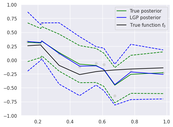
(a) LGP posterior $\Psi^{\text{L}}_{5}$.

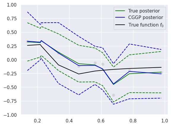
(b) CGGP posterior $\Psi^{\text{CG}}_{5}$.

Figure 1: Equivalence of LGP and CGGP for $n=10$ observations from model (7.1). LGP and CGGP posteriors $\Psi_{m}$ with $m=5$.

Then, we investigate the accuracy of the approximation resulting from different number of iterations. We recall from [VZ11] that for $f_{0}\in C^{\beta}[0,1]\cap H^{\beta}[0,1]$ and a Matérn process with $\alpha=\beta$, Assumption (CFun) holds, resulting in the minimax contraction rate $\varepsilon_{n}=n^{-\beta/(2\beta+1)}$ for the true posterior, where $C^{\beta}[0,1]$ and $H^{\beta}[0,1]$ denote the spaces of $\beta$-Hölder continuous functions and $\beta$-Sobolev functions respectively. Furthermore, Corollary 7 of [NSZ22] together with the equivalence in Lemma 4.1 guarantees that the EVGP posterior $\Psi^{\text{EV}}_{m}$ also contracts with the rate $\varepsilon_{n}=n^{-\beta/(1+2\beta)}$ as long as

$$m\geq n^{1/(1+2\beta)}\approx 40\qquad\text{ for }n=3000.$$ (7.4)

This is confirmed by the plot in Figure 2, which reproduces the results from [NSZ22]. For the empirical eigenvectors, we use the full SVD of the kernel matrix computed via linalg.svd from NumPy [Har+20].

Based on our theoretical results we can expect the same optimal contraction rate to hold for the CGGP posterior as well, as long as the Lanczos approximation of the eigenpairs of the kernel matrix is sufficient. For a Krylov space of dimension $40$, however, we cannot expect convergence for all 40 eigenpairs, which is the reason that Theorem 4.2 requires an additional slowly increasing multiplicative factor (in the theorem a logarithmic term was introduced, but a slower factor is also sufficient). Correspondingly, the CGGP posterior for $m=40$, which is equivalent to the LGP posterior with $m=40$ based on the Krylov space $\mathcal{K}_{40}$, displays slightly worse approximation behaviour than the idealized EVGP one. This slight suboptimality can be seen by the wider credible bands even if the posterior mean is already replicated close to exactly and the mean squared error (MSE)

$$\text{MSE}=\frac{1}{n}\sum_{i=1}^{n}(\mu_{m}^{\text{CG}}(X_{i})-f_{0}(X_{i}))^{2}$$ (7.5)

of the CGGP posterior mean $\mu_{m}^{\text{CG}}$ is essentially identical to the MSE of the true posterior mean, see Table 1.

To incorporate the slightly larger iteration number needed for the CG and Lanczos algorithms we also run CGGP twice as long, for $m=80$ iterations. Note that the logarithmic factor from our theorem would imply a $\log n=8$ (for $n=3000$) multiplier compared to the EVGP case. However, as discussed above, a smaller term is also sufficient. In fact, the documentation of the implementation sparse.linalg.svds of the Lanczos algorithm from SciPy [Vir+20] suggests also to use twice as large dimensional Krylov space as the number of approximated eigenpairs needed by the user to guarantee convergence. The results for the CGGP posterior with $m=80$ iterations then provide an approximation that is highly similar to the EVGP, see Figure 3 and Table 1.

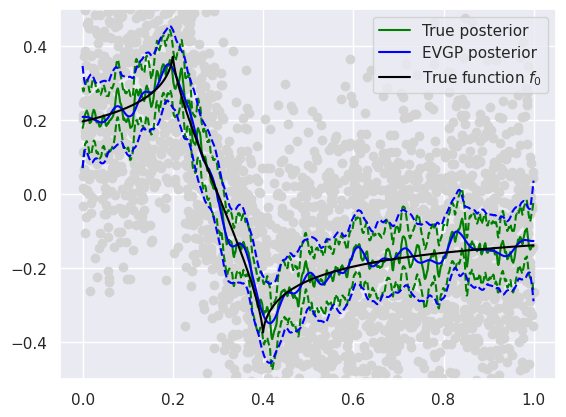
(a) EVGP $\Psi_{40}^{\text{EV}}$.

(b) CGGP $\Psi_{40}^{\text{CG}}$.

Figure 2: Simulation results for the Matern kernel with $n=3000$ observations from model (7.1). EVGP and CGGP posteriors $\Psi_{m}$ with $m=40$.

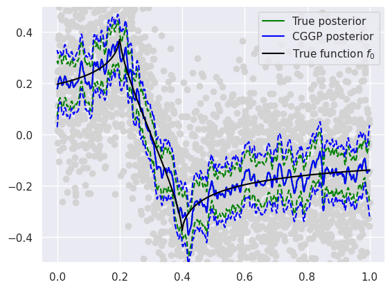
(a) CGGP $\Psi_{80}^{\text{CG}}$.

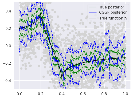
(b) CGGP $\Psi_{20}^{\text{CG}}$.

Figure 3: Simulation results for the Matern kernel with $n=3000$ observations from model (7.1). CGGP posteriors $\Psi^{\text{CG}}_{m}$ with $m=80$ and $20$, respectively.

Considering only half as many iterations than for the EVGP method, i.e., $m=20$, as suggested by our theory, results in an approximation that is substantially worse than the true posterior. This is indicated by an order of magnitude larger MSE and credible bands that are wider by about a factor of two than for the true posterior. Increasing the number of iterations substantially beyond what is suggested by our theory allows to recover the true posterior more precisely, however, without qualitatively improving the resulting inference on $f_{0}$, see Figure 4 and Table 1.

Finally, the $\log$-$\log$ plot in Figure 4 illustrates that the computational cost of the CGGP posterior with $m=2n^{1/(2\alpha+1)}$ iterations scales like $O(mn^{2})$ instead of $O(n^{3})$.

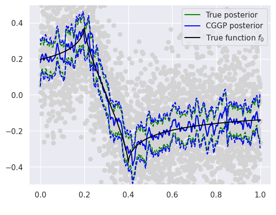
(a) CGGP $\Psi_{160}^{\text{EV}}$, MSE $=7.5\text{e}^{-04}$.

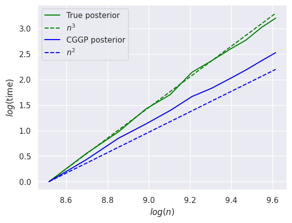
(b) Log-log plot of computation times.

Figure 4: Simulation results for the Matern kernel with $n=3000$ observations from model (7.1). CGGP posteriors $\Psi^{\text{CG}}_{m}$ with $m=160$. Log-log plot of computation times for the true posterior compared with the CGGP posterior for the optimal choice of $m$. $n\in\{5000,6000,\dots,15000\}$ and intercept shifted to $0$.

Posterior	True	$\Psi_{40}^{\text{EV}}$	$\Psi_{20}^{\text{CG}}$	$\Psi_{40}^{\text{CG}}$	$\Psi_{80}^{\text{CG}}$	$\Psi_{160}^{\text{CG}}$
MSE	$8\text{e}^{-04}$	$6\text{e}^{-04}$	$2\text{e}^{-03}$	$9\text{e}^{-04}$	$8\text{e}^{-04}$	$8\text{e}^{-04}$

Table 1: MSE for the posteriors displayed in Figures 2, 3 and 4.

7.2 Squared exponential covariance kernel

We consider the regression model (7.1) with $\sigma=0.2$ and

$$f_{0}(x):=|x+1|^{\beta}-|x-3/2|^{\beta},\qquad x\in\mathbb{R},$$ (7.6)

with regularity $\beta=0.8$. As a prior, we choose a centered GP with squared exponential covariance kernel

$$k(x,x^{\prime}):=\exp\Big{(}\frac{-(x^{\prime}-x)^{2}}{b^{2}}\Big{)},\qquad x,x^{\prime}\in\mathbb{R}.$$ (7.7)

The corresponding eigenvalues are exponentially decaying, see Section 5 for discussion and references. By setting the bandwidth parameter $b=b_{n}=4n^{-1/(1+2\beta)}$, the corresponding true posterior achieves the minimax contraction rate $\varepsilon_{n}=n^{-\beta/(1+2\beta)}$ for any $f_{0}\in C^{\beta}(\mathbb{R})\cap L^{2}(\mathbb{R})$. Since with high probability, the design points $X_{i}$, $i\leq n$ are contained in a compact interval and the tails of $f_{0}$ can be adjusted to guarantee $f_{0}\in L^{2}(\mathbb{R})$, these assumptions are essentially satisfied in our setting.

As in Section 7.1, we focus on results for the CGGP posterior after checking the equivalence between LGP and CGGP from Corollary 6.3 for small $n$ and $m$, see Figure 5.

Posterior	True	$\Psi_{80}^{\text{EV}}$	$\Psi_{40}^{\text{CG}}$	$\Psi_{80}^{\text{CG}}$	$\Psi_{160}^{\text{CG}}$	$\Psi_{320}^{\text{CG}}$
MSE	$6\text{e}^{-04}$	$6\text{e}^{-04}$	0.01	$6\text{e}^{-04}$	$6\text{e}^{-04}$	$6\text{e}^{-04}$

Table 2: MSE for the posteriors displayed in Figures 6, 7 and 8.

(a) LGP posterior $\Psi^{\text{L}}_{3}$.

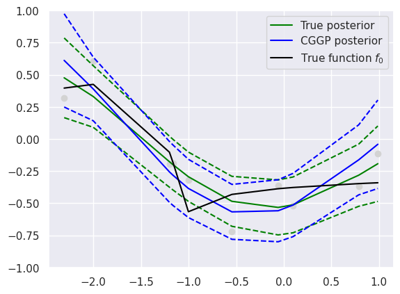
(b) CGGP posterior $\Psi^{\text{CG}}_{3}$.

Figure 5: Equivalence of LGP and CGGP for $n=10$ observations in the regression model with $f_{0}$ given in (7.6). The LGP and CGGP posteriors $\Psi_{m}$ are computed with $m=3$ iterations. The Lanczos algorithm is initialized at $w_{0}=Y/\|Y\|$.

(a) EVGP $\Psi_{80}^{\text{EV}}$

(b) CGGP $\Psi_{80}^{\text{CG}}$,

Figure 6: CGGP approximation in the regression model with $f_{0}$ given in (7.6), sample size $n=5000$ and squared exponential covariance kernel. The approximate EVGP and CGGP posteriors $\Psi_{m}$ are computed with $m=80$ iterations.

For the EVGP posterior $\Psi_{m}^{\text{EV}}$, Corollary 9 in [NSZ22] together with Lemma 4.1 guarantee that the contraction rate of the approximate posterior is (nearly) optimal $n^{-\beta/(1+2\beta)}\log n$ for a choice

$$m\geq 2^{-3/2}n^{1/(1+2\beta)}\log n\approx 80\qquad\text{for $n=5000$.}$$ (7.8)

This is confirmed in Figure 6, showing that $\Psi^{\text{EV}}_{80}$ already recovers the true posterior along the whole interval that contains the observations. The CGGP posterior provides a good approximation within two standard deviations of the standard normal design distribution, see Figure 6(b). It turns out that $m=80$ iterations are enough for the CGGP posterior mean to achieve essentially the same MSE as the true posterior, see Table 2. Following the same reasoning as in Section 7.1, we add a factor two to the iteration number. Then, the CGGP has essentially the same performance, including the width of the credible bands, as the EVGP posterior.

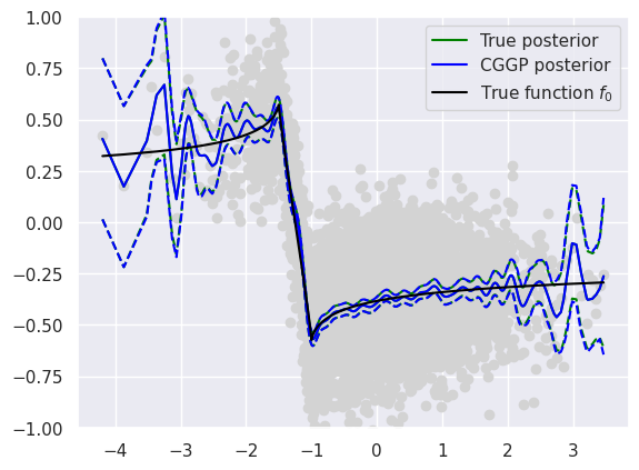
(a) CGGP $\Psi_{160}^{\text{CG}}$.

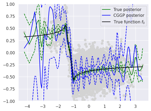
(b) EVGP $\Psi_{40}^{\text{EV}}$

Figure 7: Comparing approximation accuracy for other iteration numbers in the setting of Figure 6. The EVGP and CGGP posteriors $\Psi_{m}$ are computed with $m=160$ and $m=40$ iterations, respectively.

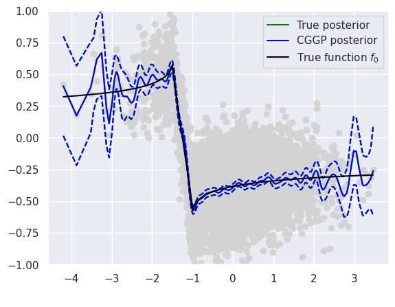
(a) CGGP $\Psi_{320}^{\text{EV}}$

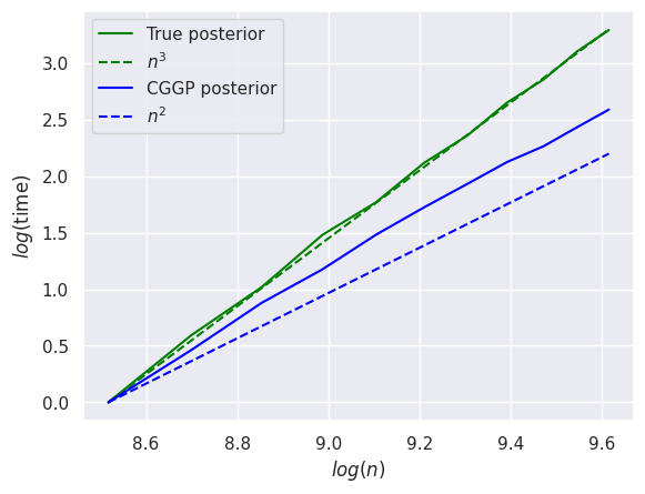
(b) Log-log plot of computation times.

Figure 8: CGGP posterior $\Psi^{\text{CG}}_{m}$ with $m=320$. Log-log plot of computation times for the true posterior compared with the CGGP posterior for the optimal choice of $m$. $n\in\{5000,6000,\dots,15000\}$ and intercept shifted to $0$.

Considering half the optimal amount of iterations $m=40$, this relationship is lost as the CGGP posterior cannot approximate the true posterior even within one standard deviation of the design distribution, see Figure 7. This is also reflected by the substantially larger MSE of the posterior mean. Finally, increasing the number of iterations beyond the indicated size, here we choose $m=320$, visually recovers the true posterior exactly, however, without improving the MSE, see Figure 8.

In conclusion, the numerical analysis above indicates that the approximate posterior, based on sufficiently many iterations, produces similarly reliable inference on the true functions $f_{0}$ while reducing the computational complexity of the procedure substantially. The amount of reduction is illustrated in Figure 8, which shows that the computation time of the true posterior scales like $O(n^{3})$, whereas the approximation scales like $O(mn^{2})$.

Appendix A Proofs of main results

Proof of Lemma 4.1 (Empirical eigenvector actions and variational Bayes).

Since two
Gaussian processes are uniquely determined by their mean and covariance functions, it suffices to check that these are equal. The mean and covariance functions of the empirical eigenvector posterior from Algorithm 1 are given by

$$x \mapsto k(X,x)^{\top}C_{m}^{\text{EV}}Y=k(X,x)^{\top}\sum_{j=1}^{m}\frac{\langle\widehat{u},Y\rangle}{\widehat{\mu}_{j}+\sigma^{2}}\widehat{u}_{j},$$ (A.1)

$$(x,x^{\prime}) \mapsto k(x,x^{\prime})-k(X,x)^{\top}C_{m}k(X,x)=k(x,x^{\prime})-\sum_{j=1}^{m}\frac{\langle k(X,x),\widehat{u}_{j}\rangle\langle k(X,x^{\prime}),\widehat{u}_{j}\rangle}{\widehat{\mu}_{j}+\sigma^{2}}.$$

By combining Equations (3.11), (3.13) and (3.15), the variational Bayes posterior mean and covariance functions, in the notation from there, are given by

$$x \mapsto\sigma^{2}K_{xu}(\sigma^{-2}K_{uf}K_{fu}+K_{uu})^{-1}K_{uf}Y$$ (A.2)

$$(x,x^{\prime}) \mapsto k(x,x^{\prime})-K_{xu}K_{uu}^{-1}K_{ux}+K_{xu}(\sigma^{-2}K_{fu}K_{uf}+K_{uu})^{-1}K_{ux}.$$

where from Equation (3.16), it follows that $K_{uu}=\text{Cov}(U)=\operatorname*{diag}(\widehat{\mu}_{1},\dots,\widehat{\mu}_{m})$,

$$K_{uf} =(\text{Cov}(U_{j},F(X_{i})))_{j\leq m,i\leq n}=\begin{pmatrix}\widehat{\mu}_{1}\widehat{u}_{1}^{\top}\\ \vdots\\ \widehat{\mu}_{m}\widehat{u}_{m}^{\top}\\ \end{pmatrix}\in\mathbb{R}^{m\times n}$$ (A.3)

$$\qquad\text{ and }\qquad K_{xu} =(\text{Cov}(F(x),U_{j}))_{j\leq m}=k(X,x)^{\top}\begin{pmatrix}\widehat{u}_{1}\dots\widehat{u}_{m}\end{pmatrix}\in\mathbb{R}^{1\times m}.$$

Consequently, the mean function is

$$x \mapsto k(X,x)^{\top}\begin{pmatrix}\vdots&&\vdots\\ \widehat{u}_{1}&\dots&\widehat{u}_{m}\\ \vdots&&\vdots\end{pmatrix}\begin{pmatrix}(\widehat{\mu}_{1}^{2}+\sigma^{2}\widehat{\mu}_{1})^{-1}&&\\ &\ddots&\\ &&(\widehat{\mu}_{m}^{2}+\sigma^{2}\widehat{\mu}_{m})^{-1}\end{pmatrix}\begin{pmatrix}\widehat{\mu}_{1}\langle Y,\widehat{u}_{1}\rangle\\ \vdots\\ \widehat{\mu}_{m}\langle Y,\widehat{u}_{m}\rangle\\ \end{pmatrix}$$

$$=k(X,x)^{\top}\sum_{j=1}^{m}\frac{\langle\widehat{u},Y\rangle}{\widehat{\mu}_{j}+\sigma^{2}}\widehat{u}_{j}.$$ (A.4)

An analogous calculation shows that also the coavariance functions coincide. ∎

Proof of Proposition 6.2 (Kullback-Leibler bound).

We pick up the reasoning at the decomposition of the Kullback-Leibler divergence from Equation (6.1). For notational convenience, we omit the dependency of $m_{n}$ and $\tilde{m}_{n}=m_{n}\log n$ on $n$.

We note that $C_{\tilde{m}}-C_{m}\geq 0$ implies

$$\operatorname*{tr}(K-KK_{\sigma}^{-1}K)^{-1}K(C_{\tilde{m}}-C_{m})K \geq 0$$ (A.5)

and

$$\ \ \ \ \|(K_{\sigma}^{-1}-C_{\tilde{m}})Y\|_{K(K-KK_{\sigma}^{-1}K)^{-1}K}=\|\Gamma_{\tilde{m}}K_{\sigma}K_{\sigma}^{-1}Y\|_{K(K-KK_{\sigma}^{-1}K)^{-1}K}$$ (A.6)

$$=\|\Gamma_{\tilde{m}}K_{\sigma}\Gamma_{m}K_{\sigma}K_{\sigma}^{-1}Y\|_{K(K-KK_{\sigma}^{-1}K)^{-1}K}\leq\|\Gamma_{m}K_{\sigma}K_{\sigma}^{-1}Y\|_{K(K-KK_{\sigma}^{-1}K)^{-1}K},$$

$$=\|(K_{\sigma}^{-1}-C_{m})Y\|_{K(K-KK_{\sigma}^{-1}K)^{-1}K},$$

where we have used the fact that $\Gamma_{m}K_{\sigma}$ is the $K_{\sigma}$-orthogonal projection onto $\operatorname*{span}\{s_{j}:j\leq m\}^{\perp}$. Using this, we may assume without loss of generality that $\operatorname*{KL}(\Psi_{\tilde{m}},\Pi_{n}(\cdot|X,Y))\leq\operatorname*{KL}(\Psi_{m},\Pi_{n}(\cdot|X,Y))$, i.e., we can consider the approximate posterior based on $(\tilde{u}_{i})_{i\leq m}$ but from the Lanczos algorithm computed based on $\tilde{m}$.

Step 1: Empirical eigenvector part. Treating the first part of the decomposition from Equation (6.3)

$$({\dagger}):=\operatorname*{tr}(K-KK_{\sigma}^{-1}K)^{-1}K(K_{\sigma}^{-1}-C_{m}^{\text{EV}})K+2\|(K_{\sigma}^{-1}-C_{m}^{\text{EV}})Y\|_{K(K-KK_{\sigma}^{-1}K)^{-1}K}^{2},$$ (A.7)

which only depends on the idealized empirical eigenvalues $(\widehat{u}_{i})_{i\leq m}$, is straightforward. The trace term satisfies

$$\ \ \ \ \operatorname*{tr}(K-KK_{\sigma}^{-1}K)^{-1}K(K_{\sigma}^{-1}-C_{m}^{\text{EV}})K$$ (A.8)

$$=\operatorname*{tr}(K-KK_{\sigma}^{-1}K)^{-1}\Big{(}\sum_{j=m+1}^{n}\frac{\widehat{\mu}_{j}^{2}}{\widehat{\mu}_{j}+\sigma^{2}}\widehat{u}_{j}\widehat{u}_{j}^{\top}\Big{)}=\frac{n}{\sigma^{2}}\sum_{j=m+1}^{n}\widehat{\lambda}_{j},$$

since the matrix $(K-KK_{\sigma}^{-1}K)$ can also be decomposed in terms of the projectors $(\widehat{u}_{j}\widehat{u}_{j}^{\top})_{j\leq n}$ with eigenvalues

$$\Big{(}\widehat{\mu}_{j}-\frac{\widehat{\mu}_{j}^{2}}{\widehat{\mu}_{j}+\sigma^{2}}\Big{)}=\frac{\widehat{\mu}_{j}\sigma^{2}}{\widehat{\mu}_{j}+\sigma^{2}}\qquad\text{ for all }j\leq n.$$ (A.9)

For the term involving $Y=\mathbf{f}_{0}+\varepsilon$, we set $\Gamma_{m}^{\text{EV}}:=K_{\sigma}^{-1}-C_{m}^{\text{EV}}$ and estimate

$$\ \ \ \ \|(K_{\sigma}^{-1}-C_{m}^{\text{EV}})Y\|_{K(K-KK_{\sigma}^{-1}K)K}^{2}=Y^{\top}\Gamma^{\text{EV}}_{m}K(K-KK_{\sigma}^{-1}K)^{-1}K\Gamma_{m}^{\text{EV}}Y$$

$$\leq 2\mathbf{f}_{0}^{\top}\Gamma_{m}^{\text{EV}}K(K-KK_{\sigma}^{-1}K)^{-1}K\Gamma_{m}^{\text{EV}}\mathbf{f}_{0}+2\varepsilon^{\top}\Gamma_{m}^{\text{EV}}K(K-KK_{\sigma}^{-1}K)^{-1}K\Gamma_{m}^{\text{EV}}\varepsilon.$$

We further split $\mathbf{f}_{0}:=\mathbf{h}+\mathbf{f}_{0}-\mathbf{h}$, where $h\in\mathbb{H}$ is an element of the RKHS induced by the prior process and estimate both individually again. Then,

$$\ \ \ \ \mathbf{h}^{\top}\Gamma_{m}^{\text{EV}}K(K-KK_{\sigma}^{-1}K)^{-1}K\Gamma_{m}^{\text{EV}}\mathbf{h}$$ (A.10)

$$=\mathbf{h}^{\top}K_{\sigma}^{-1}(I-K_{\sigma}C_{m}^{\text{EV}})K(K-KK_{\sigma}^{-1}K)^{-1}K\Gamma_{m}^{\text{EV}}\mathbf{h}$$

$$\leq\mathbf{h}^{\top}K_{\sigma}^{-1}\mathbf{h}\|(I-K_{\sigma}C_{m}^{\text{EV}})K(K-KK_{\sigma}^{-1}K)^{-1}K\Gamma_{m}^{\text{EV}}\|_{\text{op}}$$ (A.11)

$$\leq\|h\|_{\mathbb{H}}^{2}\|K(K-KK_{\sigma}^{-1}K)^{-1}K\Gamma_{m}^{\text{EV}}\|_{\text{op}}\leq\frac{n}{\sigma^{2}}\|h\|_{\mathbb{H}}^{2}\widehat{\lambda}_{m+1},$$

where we have used the fact that $h^{\top}K_{\sigma}^{-1}h\leq\|P_{n,k}h\|_{\mathbb{H}}$ with $P_{n,k}$ the projection onto $\operatorname*{span}\{k(X_{i},\cdot):i=1,\dots,n\}$ and the singular value decomposition of $K(K-KK_{\sigma}^{-1}K)^{-1}K\Gamma_{m}^{\text{EV}}$.

An analogous estimate shows

$$\ \ \ \ (\mathbf{f}_{0}-\mathbf{h})^{\top}\Gamma_{m}^{\text{EV}}K(K-KK_{\sigma}^{-1}K)^{-1}K\Gamma_{m}^{\text{EV}}(\mathbf{f}_{0}-\mathbf{h})$$ (A.12)

$$\leq n\|f_{0}-h\|_{n}^{2}\|\Gamma_{m}^{\text{EV}}K(K-KK_{\sigma}^{-1}K)^{-1}K\Gamma_{m}^{\text{EV}}\|_{\text{op}}\leq\frac{n}{\sigma^{2}}\|f_{0}-h\|_{n}^{2}.$$

Plugging all estimates into Equation (A.7) yields that

$$({\dagger}) \leq\frac{Cn}{\sigma^{2}}\Big{(}\sum_{j=m+1}^{n}\widehat{\lambda}_{j}+\|h\|_{\mathbb{H}}^{2}\widehat{\lambda}_{m+1}+\|f_{0}-h\|_{n}^{2}\Big{)}$$ (A.13)

$$+2\varepsilon^{\top}\Gamma^{\text{EV}}_{m}K(K-KK_{\sigma}^{-1}K)^{-1}K\Gamma_{m}^{\text{EV}}\varepsilon$$

for any $h\in\mathbb{H}$.

Step 2: Lanczos eigenvector part. We treat the second part of the decomposition in Equation (6.1)

$$({\dagger}{\dagger}):=\operatorname*{tr}(K-KK_{\sigma}^{-1}K)^{-1}K(C^{\text{EV}}_{m}-C_{m})K+2\|(C_{m}-C^{\text{EV}}_{m})Y\|_{K(K-KK_{\sigma}^{-1}K)K}^{2},$$ (A.14)

with $C_{m}=C_{m}^{\text{L}}$ and set $D_{m}:=C_{m}^{\text{EV}}-C_{m}^{\text{L}}$. The trace term satisfies

$$\ \ \ \ \operatorname*{tr}(K-KK_{\sigma}^{-1}K)^{-1}K(C^{\text{EV}}_{m}-C_{m}^{\text{L}})K=\operatorname*{tr}K(K-KK_{\sigma}^{-1}K)^{-1}KD_{m}$$ (A.15)

$$\leq\|K(K-KK_{\sigma}^{-1}K)^{-1}K\|_{HS}\|D_{m}\|_{\text{HS}}\leq\frac{n(\|K\|_{\text{op}}^{2}+\sigma^{2}\|K\|_{\text{op}})}{\sigma^{2}}\|D_{m}\|_{\text{HS}},$$

where we have used the singular value decomposition of $K$ again.

For the other term, we again split $Y=\mathbf{f}_{0}-\mathbf{h}+\mathbf{h}+\mathbf{\varepsilon}$ for an arbitrary element $h\in\mathbb{H}$ and estimate

$$\ \ \ \ \|(C_{m}^{\text{L}}-C_{m}^{\text{EV}})Y\|_{K(K-KK_{\sigma}^{-1}K)K}^{2}$$ (A.16)

$$\leq C\|K(K-KK_{\sigma}^{-1}K)K\|_{\text{op}}(\|\varepsilon\|^{2}+n\|f_{0}-h\|_{n}^{2}+\|\mathbf{h}\|^{2})\|D_{m}\|_{\text{HS}}^{2}$$ (A.17)

$$\leq C\frac{\|K\|_{\text{op}}^{2}+\sigma^{2}\|K\|_{\text{op}}}{\sigma^{2}}(\|\varepsilon\|^{2}+n\|f_{0}-h\|_{n}^{2}+(\|K\|_{\text{op}}+\sigma^{2})\|h\|_{\mathbb{H}})\|D_{m}\|_{\text{HS}}^{2},$$

where we have used again that $\|\mathbf{h}\|^{2}\leq(\|K\|_{\text{op}}+\sigma^{2})\|K_{\sigma}^{-1/2}\mathbf{h}\|^{2}\leq(\|K\|_{\text{op}}+\sigma^{2})\|h\|_{\mathbb{H}}^{2}$. Together, this yields

$$({\dagger}{\dagger}) \leq C\Big{(}\frac{n(\|K\|_{\text{op}}^{2}+\sigma^{2}\|K\|_{\text{op}})}{\sigma^{2}}\|D_{m}\|_{\text{HS}}$$ (A.18)

$$\qquad+\frac{\|K\|_{\text{op}}^{2}+\sigma^{2}\|K\|_{\text{op}}}{\sigma^{2}}(\|\varepsilon\|^{2}+n\|f_{0}-h\|_{n}^{2}+(\|K\|_{\text{op}}+\sigma^{2})\|h\|_{\mathbb{H}}^{2})\|D_{m}\|_{\text{HS}}^{2}\Big{)}$$

for any $h\in\mathbb{H}$.

Step 3: Probabilistic part. Via Markov’s inequality, for a fixed sequence $M_{n}\to\infty$, we can restrict to an event with probability converging to one, on which

$$\sum_{j=m+1}^{n}\widehat{\lambda}_{j}\leq M_{n}\sum_{j=m+1}^{n}\lambda_{j},\quad\widehat{\lambda}_{m+1}\leq M_{n}\mathbb{E}\widehat{\lambda}_{m+1},\quad\|f_{0}-h\|_{n}^{2}\leq M_{n}\|f_{0}-h\|_{L^{2}}^{2},$$ (A.19)

where we have also used Proposition B.6 for the first inequality. By the same reasoning, we can also assume that

$$\ \ \ \ \varepsilon^{\top}\Gamma_{m}^{\text{EV}}K(K-KK_{\sigma}^{-1}K)^{-1}K\Gamma_{m}^{\text{EV}}\varepsilon\leq M_{n}\mathbb{E}_{\varepsilon}\operatorname*{tr}(\varepsilon\varepsilon^{\top})\Gamma_{m}^{\text{EV}}K(K-KK_{\sigma}^{-1}K)^{-1}K\Gamma_{m}^{\text{EV}}$$

$$=M_{n}\sigma^{2}\operatorname*{tr}\Gamma_{m}^{\text{EV}}K(K-KK_{\sigma}^{-1}K)^{-1}K\Gamma_{m}^{\text{EV}}\leq\frac{M_{n}n}{\sigma^{2}}\sum_{j=m+1}^{n}\widehat{\lambda}_{j}$$ (A.20)

and $\|\varepsilon\|^{2}\leq M_{n}\mathbb{E}\|\varepsilon\|^{2}=M_{n}\sigma^{2}n$.

By further restricting to the event from Proposition 6.9 with $m_{0}=C\tilde{m}=Cm\log n$ and using Proposition 6.10, we finally have

$$\|D_{m}\|_{\text{HS}} \leq\sum_{j=1}^{m}\Big{\|}\frac{1}{\widehat{\mu}_{j}+\sigma^{2}}\widehat{u}_{j}\widehat{u}_{j}^{\top}-\frac{1}{\tilde{\mu}_{j}+\sigma^{2}}\tilde{u}_{j}\tilde{u}_{j}^{\top}\Big{\|}_{\text{HS}}$$ (A.21)

$$\leq\sum_{j=1}^{m}\Big{|}\frac{1}{\widehat{\mu}_{j}+\sigma^{2}}-\frac{1}{\tilde{\mu}_{j}+\sigma^{2}}\Big{|}+\frac{\|\widehat{u}_{j}\widehat{u}_{j}^{\top}-\tilde{u}_{j}\tilde{u}_{j}^{\top}\|_{\text{HS}}}{\sigma^{2}}$$

$$\leq\Big{(}\frac{mn}{\sigma^{4}}+\frac{m}{\sigma^{2}}\Big{)}(1+c)^{-m}$$

and $\|K\|_{\text{op}}=\widehat{\mu}_{1}=n\widehat{\lambda}_{1}\leq Cn\lambda_{1}$ as in Step 1 of the proof of Proposition 6.10.

Now, Assumption (CFUN) implies that we can choose $h\in\mathbb{H}$ such that

$$\|h\|_{\mathbb{H}}^{2}\leq n\varepsilon_{n}^{2}\qquad\text{ and }\qquad\|f_{0}-h\|_{L^{2}}^{2}\leq\varepsilon_{n}^{2}.$$ (A.22)

In combining all of our estimates, we note that since $C^{\prime}\log n\leq m$ for $C^{\prime}$ sufficiently large, all terms involving $\|D_{m}\|_{\text{HS}}$ are of lower order. The remaining terms yield the estimate

$$\operatorname*{KL}(\Psi_{\tilde{m}},\Pi_{n}(\cdot|X,Y)) \leq({\dagger})+({\dagger}{\dagger})\leq\frac{CM_{n}^{2}n}{\sigma^{2}}\Big{(}\varepsilon_{n}^{2}+\sum_{j=m+1}^{\infty}\lambda_{j}+n\varepsilon_{n}^{2}\mathbb{E}\widehat{\lambda}_{m+1}\Big{)}.$$ (A.23)

The result now follows by adjusting the sequence $M_{n}$ accordingly. This finishes the proof. ∎

Proof of Corollary 6.3 (Equivalence between LGP and CGGP).

The approximate posterior from Algorithm 1 only depends on the approximation $C_{m}$ of $K_{\sigma}^{-1}$. Additionally, since $C_{m}K_{\sigma}^{-1}$ is the $K_{\sigma}^{-1}$-orthogonal projection onto $\operatorname*{span}\{s_{j}:j\leq m\}$, see Lemma S1 in [Wen+22], $C_{m}$ only depends on $\operatorname*{span}\{s_{j}:j\leq m\}$. Consequently, if for two versions of the algorithm $\operatorname*{span}\{s_{j}:j\leq m\}$ coincide, then the resulting approximate posteriors are identical.

Now, for the Lanczos algorithm initiated at $Y/\|Y\|$ iterated for $m$ steps

$$\operatorname*{span}\{s_{j}:j\leq m\}=\operatorname*{span}\{\tilde{u}_{j}:j\leq m\}=\operatorname*{span}\{Y,KY,\dots K^{m-1}Y\}$$ (A.24)

and since the conjugate gradients of the CG-method span the Krylov space associated with $K_{\sigma}$ and $Y$, we also have

$$\operatorname*{span}\{s_{j}:j\leq m\}=\operatorname*{span}\{Y,K_{\sigma}Y,\dots,K_{\sigma}^{m-1}Y\}=\operatorname*{span}\{Y,KY,\dots K^{m-1}Y\}.$$

This proves that the resulting approximate posteriors are identical. The last statement of Corollary 6.3 then follows immediately. ∎

Appendix B Auxiliary results

Lemma B.1 (Multivariate conditional Gaussians).

For a random variable $(X,Y)^{\top}\in\mathbb{R}^{m+n}$ with joint distribution

$$\begin{pmatrix}X\\ Y\end{pmatrix}\sim N\left(\begin{pmatrix}\mu\\ \nu\end{pmatrix},\begin{pmatrix}R&C\\ C^{\top}&S\end{pmatrix}\right)$$ (B.1)

where $R$ is nonsingular, the conditional distribution $Y|X$ is given by $N(\nu+C^{\top}(X-\mu),S-C^{\top}R^{-1}C)$.

Proof.

See Proposition 3.13 in [Eat07]. ∎

Proof of Lemma 2.2 (EVGP).

We establish the claim via induction over $m\in\mathbb{N}$. For $m=1$, the definition of Algorithm 1 states that

$$d_{1}=(I-0\cdot K_{\sigma})s_{1}=\widehat{u}_{1},\qquad\text{ and }\qquad\eta_{1}=\widehat{u}_{1}^{\top}K_{\sigma}\widehat{u}_{1}=\widehat{\mu}_{1}+\sigma^{2},$$ (B.2)

which yields $C^{\text{EV}}_{1}=(\widehat{\mu}_{1}+\sigma^{2})^{-1}\widehat{u}_{1}\widehat{u}_{1}^{\top}$. Suppose now that we have shown the claim for $m$. Then, we obtain

$$d_{m+1}=(I-C_{m}^{\text{EV}}K_{\sigma})\widehat{u}_{m+1}=\widehat{u}_{m+1}\quad\text{ and }\quad\eta_{m+1}=\widehat{u}_{m+1}^{\top}K_{\sigma}\widehat{u}_{m+1}=\widehat{\mu}_{m+1}+\sigma^{2},$$ (B.3)

where we have used that $C^{\text{EV}}_{m}=\sum_{j=1}^{m}(\widehat{\mu}_{j}+\sigma^{2})^{-j}\widehat{u}_{j}\widehat{u}_{j}^{\top}$. This finishes the proof. ∎

Proof of Lemma 2.3 (LGP).

We establish the result via induction over $m\in\mathbb{N}$. For $m=1$, the definition of Algorithm 1 and Lemma 6.6 (ii) yield that

$$d_{1}=s_{1}=\tilde{u}_{1}\qquad\text{ and }\qquad\eta_{1}=\tilde{u}_{1}^{\top}K_{\sigma}\tilde{u}_{1}=(\tilde{\mu}_{1}+\sigma^{2})\tilde{u}_{1}^{\top}(\tilde{u}_{1}+u^{\perp})=\tilde{\mu}_{1}+\sigma^{2},$$ (B.4)

for some $u^{\perp}\perp\mathcal{K}_{\tilde{m}}$.

Suppose, we have established the claim for $m\in\mathbb{N}$. Then, we obtain

$$d_{m+1} =(I-C_{m}^{\text{L}}K_{\sigma})\tilde{u}_{m+1}=\tilde{u}_{m+1}-C_{m}^{\text{L}}((\tilde{\mu}_{m+1}+\sigma^{2})\tilde{u}_{m+1}+u_{1}^{\perp})=\tilde{u}_{m+1},$$ (B.5)

$$\eta_{m+1} =\tilde{u}_{m+1}^{\top}K_{\sigma}\tilde{u}_{m+1}=\tilde{u}_{m+1}^{\top}((\widehat{\mu}_{m+1}+\sigma^{2})\tilde{u}_{m+1}+u_{2}^{\perp})=\widehat{\mu}_{m+1}+\sigma^{2},$$

where again, $u_{1}^{\perp},u_{2}^{\perp}$ are elements in $\mathcal{K}_{m}^{\perp}$ and we have used that $C^{\text{L}}_{m}=\sum_{j=1}^{m}(\tilde{\mu}_{j}+\sigma^{2})^{-j}\tilde{u}_{j}\tilde{u}_{j}^{\top}$. ∎

Proof of Lemma 2.4 (CGGP).

We establish the result via induction over $m\in\mathbb{N}$. For $m=1$, the definition of Algorithm 1 yields that

$$d_{1}=s_{1}=d_{1}^{\text{CG}}\qquad\text{ and }\qquad\eta_{1}=(d_{1}^{\text{CG}})^{\top}K_{\sigma}d_{1}^{\text{CG}}$$ (B.6)

Suppose, we have established the claim for $m\in\mathbb{N}$. Then, we obtain

$$d_{m+1}=(I-C_{m}^{\text{CG}}K_{\sigma})d_{m+1}^{\text{CG}}=d_{m+1}^{\text{CG}}\qquad\text{ and }\qquad\eta_{m+1}=(d_{m+1}^{\text{CG}})^{\top}K_{\sigma}d_{m+1}^{\text{CG}},$$ (B.7)

where we have used that $C_{m}^{\text{CG}}=\sum_{j=1}^{m}((d_{j}^{\text{CG}})^{\top}K_{\sigma}d_{j}^{\text{CG}})^{-1}d_{j}^{\text{CG}}(d_{j}^{\text{CG}})^{\top}$ and the conjugacy condition from Equation (2.15). ∎

Lemma B.2 (KL between posterior processes).

Conditional on the design $X$ and the observations $Y$, the Kullback-Leibler divergence $\operatorname*{KL}(\Psi_{m},\Pi_{n}(\cdot|X,Y))$ between the approximate posterior GP from Algorithm 1 and the true posterior GP is equal to the Kullback-Leibler divergence $\operatorname*{KL}(\Psi_{m}\{\mathbf{f}\in\cdot\},\Pi_{n}\{\mathbf{f}\in\cdot|X,Y\}))$ between the finite dimensional Gaussians given by $\mathbf{f}=(f(X_{1}),\dots f(X_{n}))$, i.e., the function $f$ evaluated at the design points.

Proof.

Initially, we introduce some helpful notation. Let $(\Omega,\mathscr{A},\mathbb{P})$ denote the probability space on which the Gaussian regression model from Equation (1.1) is defined conditional on the design $X$. In the following, superscripts will denote push forward measures, see the remarks on notation in Section 1. Let $W^{*}=K_{\sigma}^{-1}Y$ denote the true representer weights and without loss of generality assume that on $(\Omega,\mathscr{A},\mathbb{P})$ there exists a random variable $W_{m}\sim N(C_{m}Y,\Gamma_{m})$ representing our believes at iteration $m$ of the Bayesian updating scheme in Equations (2.5) and (2.6). The approximate posterior $\Psi_{m}$ is the push forward of $F$ under the measure

$$\mathbb{Q}(A):=\int\mathbb{P}(A|W^{*}=w)\,\mathbb{P}^{W_{m}}(dw),\qquad A\in\mathscr{A},$$ (B.8)

i.e., $\Psi_{m}=\mathbb{Q}^{F}$.

Assuming all quantities exist, we may now write the Kullback-Leibler divergence in terms of Radon-Nikodym derivatives, i.e.,

$$\operatorname*{KL}(\Psi_{m},\Pi_{n}(\cdot|X,Y)) =\int\frac{d\Psi_{m}}{d\Pi}\,d\Psi_{m}+\int\frac{d\Pi}{d\Pi_{n}(\cdot|X,Y)}\,d\Psi_{m}$$ (B.9)

$$=\int\frac{d\mathbb{Q}^{F}}{d\mathbb{P}^{F}}\,d\mathbb{Q}^{F}+\int\frac{d\mathbb{P}^{F}}{d\mathbb{P}^{F|Y}}\,d\mathbb{Q}^{F}$$

and analogously

$$\operatorname*{KL}(\Psi_{m}\{\mathbf{f\in\cdot}\},\Pi_{n}\{\mathbf{f}\in\cdot|X,Y\}) =\int\frac{d\mathbb{Q}^{\vec{F}}}{d\mathbb{P}^{\vec{F}}}\,d\mathbb{Q}^{\vec{F}}+\int\frac{d\mathbb{P}^{\vec{F}}}{d\mathbb{P}^{\vec{F}|Y}}\,d\mathbb{Q}^{\vec{F}},$$ (B.10)

where $\vec{F}:=(F(X_{1}),\dots,F(X_{n}))$ denotes the finite dimensional evaluation of the process $F$. Therefore, it is sufficient to show that the integrands in Equations (B.9) and (B.10) and exist and coincide respectively.

For the first integrand, we initially note that $\mathbb{Q}$ is absolutely continuous with respect to $\mathbb{P}$ with

$$\frac{d\mathbb{Q}}{d\mathbb{P}}=\Big{(}\frac{d\mathbb{P}^{W_{m}}}{d\mathbb{P}^{W^{*}}}\Big{)}\circ W^{*},$$ (B.11)

where $d\mathbb{P}^{W_{m}}/d\mathbb{P}^{W^{*}}=d\mathbb{Q}^{W_{m}}/d\mathbb{P}^{W^{*}}$ exists, since under $\mathbb{P}$ both $W_{m}$ and $W^{*}$ are non-degenerate Gaussians. For Equation (B.11), consider that indeed, for any $A\in\mathscr{A}$, we have

$$\ \ \ \ \int_{A}\frac{d\mathbb{P}^{W_{m}}}{d\mathbb{P}^{W^{*}}}(W^{*})\,d\mathbb{P}=\int\frac{d\mathbb{P}^{W_{m}}}{d\mathbb{P}^{W^{*}}}(w)\,\mathbb{P}(A|W^{*}=w)\mathbb{P}^{W^{*}}(dw)=\mathbb{Q}(A).$$ (B.12)

This can now be used to prove $d\mathbb{Q}^{F}/d\mathbb{P}^{F}=d\mathbb{Q}^{\vec{F}}/d\mathbb{P}^{\vec{F}}$: For any Borel set $B\subset L^{2}(G)$,

$$\mathbb{Q}\{F\in B\} =\int_{F\in B}\frac{d\mathbb{Q}^{W_{m}}}{d\mathbb{P}^{W^{*}}}(W^{*})\,d\mathbb{P}=\iint\mathbf{1}_{B}(f)\frac{d\mathbb{Q}^{W_{m}}}{d\mathbb{P}^{W^{*}}}(K_{\sigma}^{-1}(\mathbf{f}+\varepsilon))\,\mathbb{P}^{\varepsilon}(d\varepsilon)\,\mathbb{P}^{F}(df),$$ (B.13)

where we have used the fact that $W^{*}=K_{\sigma}^{-1}Y$ is a function of $\mathbf{f}$ and $\varepsilon$. This implies

$$\frac{d\mathbb{Q}^{F}}{d\mathbb{P}^{F}} =\int\frac{d\mathbb{Q}^{W_{m}}}{d\mathbb{P}^{W^{*}}}(\mathbf{f}+\varepsilon)\,\mathbb{P}^{\varepsilon}(d\varepsilon),$$ (B.14)

which only depends on $\mathbf{f}=f(X_{1},\dots,X_{n})$. It follows that for any Borel set $B\subset\mathbb{R}^{n}$,

$$\int_{B}\frac{d\mathbb{Q}^{F}}{d\mathbb{P}^{F}}(\mathbf{f})\,d\mathbb{P}^{\vec{F}}(d\mathbf{f}) =\int\mathbf{1}_{B}(\mathbf{f})\frac{d\mathbb{Q}^{F}}{d\mathbb{P}^{F}}(f)\,d\mathbb{P}^{F}(df)=\mathbb{Q}\{\vec{F}\in B\},$$ (B.15)

which establishes existence and equality of the first integrands.

An analogous argument applies for the second integrands, since

$$\frac{d\mathbb{P}^{F}}{d\mathbb{P}^{F|Y}} =\Big{(}\frac{d\mathbb{P}^{F|Y}}{d\mathbb{P}^{F}}\Big{)}^{-1}=\frac{p(Y)}{p(Y|F)}=\frac{p(Y)}{p(Y|\vec{F})},$$ (B.16)

where $p$ is the likelihood of our model and we have used the fact that distribution of $Y$ only depends on $F$ evaluated at the design. ∎

Proof of Lemma 6.5 (Krylov space dimension).

We prove the linear independence of the vectors spanning the Krylov space. From the linear independence of the $(\widehat{u}_{j})_{j\leq n}$, it follows that for any $\beta\in\mathbb{R}^{\tilde{m}}$,

$$0=\sum_{k=0}^{\tilde{m}-1}\beta_{k}K^{k}v_{0} =\sum_{j=1}^{n}\langle v_{0},\widehat{u}_{j}\rangle\sum_{k=0}^{\tilde{m}-1}\beta_{k}\widehat{\lambda}_{j}^{k}\widehat{u}_{j},$$ (B.17)

implies that $\sum_{k=0}^{\tilde{m}-1}\beta_{k}\widehat{\lambda}_{j}^{k}=0$ for all $j\leq\tilde{m}$. This can be written as $\Lambda\beta=0$, where $\Lambda=(\widehat{\lambda}_{j}^{k})_{j,k}\in\mathbb{R}^{\tilde{m}\times\tilde{m}}$ is a Vandermonde matrix. Since $\widehat{\lambda}_{1}>\dots>\widehat{\lambda}_{\tilde{m}}>0$, $\Lambda$ is invertible, which implies $\beta=0$. ∎

Lemma B.3 (Convex function decay, [CMS07]).

Assume that there is a convex function $\lambda:[0,\infty)\to[0,\infty)$ such that $\lambda_{j}=\lambda(j)$ and $\lim_{j\to\infty}\lambda(j)=0$. Then, for a fixed $m$

$$\sum_{k\neq m}\frac{\lambda_{k}}{|\lambda_{m}-\lambda_{k}|} \leq Cm\log m\qquad\text{ and }\qquad\lambda_{j}-\lambda_{k}\geq\Big{(}1-\frac{j}{k}\Big{)}\lambda_{j}$$ (B.18)

for all $j<k$.

Lemma B.4 (Well definedness of the Krylov space).

Under Assumptions (SPE), (EVD) and (KLMom), consider $m$ such that $m=o((\sqrt{n}/\log n)\land(n^{(p/4-1)/2}(\log n)^{p/8-1}))$. Then, the following hold:

1. The empirical eigenvalues satisfy $\widehat{\lambda}_{1}>\widehat{\lambda}_{2}>\dots>\widehat{\lambda}_{\tilde{m}}>0$ with probability converging to one.

2. For $v_{0}:=Z/\|Z\|$, where $Z\sim N(0,I)$ independent of everything else, the tangens of the acute angles between $v_{0}$ and $(\widehat{u}_{i})_{i\leq\tilde{m}}$ satisfies

   $$0\leq\tan(v_{0},\widehat{u}_{i})\leq Cn^{2}\qquad\text{ for all }i\leq\tilde{m}$$ (B.19)

   with probability converging to one.

3. As long as $f_{0}\in L^{\infty}(G)$, the same result as in (ii) also holds for $v_{0}:=Y/\|Y\|$.

In particular, in both the settings of (ii) and (iii), Assumption (LWdf) is satisfied with probability converging to one.

Proof.

For (i), assume that there exists an $i<\tilde{m}$ such that $\widehat{\lambda}_{i}=\widehat{\lambda}_{i+1}$. Then, for $m_{0}=C\tilde{m}=Cm\log n$ in Proposition 6.9, the relative rank $\mathbf{r}_{i}$ satisfies the bound

$$\mathbf{r}_{i}\leq C\tilde{m}\log\tilde{m}\leq C\sqrt{\frac{n}{\log n}}\qquad\qquad\text{ for all }i\leq\tilde{m}$$ (B.20)

according to Lemma B.3 and our assumption on $m$. Consequently, there is an event with probability converging to one on which

$$\frac{\lambda_{i}-\lambda_{i+1}}{\lambda_{i}} \leq\Big{|}\frac{\widehat{\lambda}_{i}-\lambda_{i}}{\lambda_{i}}\Big{|}+\Big{|}\frac{\widehat{\lambda}_{i+1}-\lambda_{i+1}}{\lambda_{i}}\Big{|}\leq C\sqrt{\frac{\log n}{n}}.$$ (B.21)

At the same time, however, Lemma B.3 guarantees that $(\lambda_{i}-\lambda_{i+1})/\lambda_{i}\geq 1-i/(i+1)\geq 1/\tilde{m}$. This contradicts that by our assumptions, $\tilde{m}=o(\sqrt{n/\log n})$. Similarly, $\widehat{\lambda}_{\tilde{m}}=0$ implies that $\lambda_{\tilde{m}}\leq\lambda_{\tilde{m}}C\sqrt{\log(n)/n}$, which contradicts Assumption (SPE) for $n$ sufficiently large.

For (ii), fix $i\leq\tilde{m}$ and $t>0$. We then have $\tan(v_{0},\widehat{u}_{i})\leq 1/\cos(v_{0},\widehat{u}_{i})$ and since we are considering the acute angle $\cos(v_{0},\widehat{u}_{i})=|\langle v_{0},\widehat{u}_{i}\rangle|$. With $v_{0}=Z/\|Z\|$, we have

$$\mathbb{P}\{|\langle v_{0},\widehat{u}_{i}\rangle|\leq t\} \leq\mathbb{P}\{|\langle Z,\widehat{u}_{i}\rangle|\leq 2\sqrt{n}t\}+\mathbb{P}\{\|Z\|\geq 2\sqrt{n}\}.$$ (B.22)

Since $\|Z\|-\sqrt{n}$ is subgaussian, see [Ver18], the second probability is smaller than $\exp(-cn)$ and since $\langle Z,\widehat{u}_{i}\rangle\sim N(0,\|\widehat{u}_{i}\|^{2})$, the first probability is

$$\frac{1}{\sqrt{2\pi}}\int_{-2\sqrt{n}t}^{2\sqrt{n}t}e^{\frac{-x^{2}}{2}}\,dx\leq c\sqrt{n}t.$$ (B.23)

The result now follows from setting $t=n^{-2}$ and applying a union bound noting that $\tilde{m}n^{-3/2}\to 0$.

For (iii), analogously,

$$\mathbb{P}\{|\langle v_{0},\widehat{u}_{i}\rangle|\leq t\} \leq\mathbb{P}\{|\langle\mathbf{f}_{0}+\boldsymbol{\varepsilon},\widehat{u}_{i}\rangle|\leq C(\|f_{0}\|_{L^{2}}\lor\sigma)\sqrt{n}t\}$$ (B.24)

$$+\mathbb{P}\{\|\mathbf{f}_{0}+\boldsymbol{\varepsilon}\|\geq C(\|f_{0}\|_{L^{2}}\lor\sigma)\sqrt{n}\}$$

$$=:(\text{I})+(\text{II}).$$

Via independence, the first term satisfies

$$(\text{I}) =\int\mathbb{P}^{\varepsilon}\{|\langle\mathbf{f}_{0}+\boldsymbol{\varepsilon},\widehat{u}_{i}\rangle|\leq C(\|f_{0}\|_{L^{2}}\lor\sigma)\sqrt{n}t\}\,d\mathbb{P}^{X_{1},\dots,X_{n}}$$ (B.25)

$$=\int N(\langle\mathbf{f}_{0},\widehat{u}_{i}\rangle,\sigma^{2})([-C(\|f_{0}\|_{L^{2}}\lor\sigma)\sqrt{n}t,C(\|f_{0}\|_{L^{2}}\lor\sigma)\sqrt{n}t])\,d\mathbb{P}^{X_{1},\dots,X_{n}}$$

$$\leq\int N(0,\sigma^{2})([-C(\|f_{0}\|_{L^{2}}\lor\sigma)\sqrt{n}t,C(\|f_{0}\|_{L^{2}}\lor\sigma)\sqrt{n}t])\,d\mathbb{P}^{X_{1},\dots,X_{n}}$$

$$\leq C(\|f_{0}\|_{L^{2}}/\sigma+1)\sqrt{n}t.$$

The second term can be estimated via

$$(\text{II}) \leq\mathbb{P}\{\|\boldsymbol{\varepsilon}/\sigma\|\geq C\sqrt{n}\}+\mathbb{P}\{\|f_{0}\|_{n}^{2}-\|f_{0}\|_{L^{2}}^{2}\geq C\|f_{0}\|_{L^{2}}^{2}\}$$ (B.26)

$$\leq e^{-cn}+\exp\Big{(}\frac{-cn\|f_{0}\|_{L^{2}}^{4}}{\|f_{0}\|_{\infty}^{4}}\Big{)},$$

using the Gaussianity of $\boldsymbol{\varepsilon}$ as before and the norm concentration result in [Wai19] after Equation (14.2). The result now follows exactly as in the setting of $v_{0}=Z/\|Z\|$. ∎

Lemma B.5 (Eigenvector product terms).

Under Assumptions (SPE), (EVD) and (KLMom), consider $m=o((\sqrt{n}/\log n)\land(n^{(p/4-1)/2}(\log n)^{p/8-1}))$. Then for $\tilde{p}=m$ in Theorems 6.7 and 6.8, there exist constants $c,C>0$ such that

$$\gamma_{i}\geq 1+c,\qquad\kappa_{i}\leq C^{i}\qquad\text{ and }\qquad\kappa_{i,m}\leq C^{m}\qquad\text{ for all }i\leq m$$ (B.27)

with probability converging to one.

Proof.

As in Lemma B.4, we consider the event from Proposition 6.9 with $m_{0}=C\tilde{m}=Cm\log n$.

For $\gamma_{i}=1+2(\widehat{\lambda}_{i}-\widehat{\lambda}_{i+m+1})/(\widehat{\lambda}_{i+m+1}-\widehat{\lambda}_{n})$, the relative perturbation bound yields

$$\frac{\widehat{\lambda}_{i}-\widehat{\lambda}_{i+m+1}}{\widehat{\lambda}_{i+m+1}-\widehat{\lambda}_{n}} \geq\frac{\lambda_{i}-\lambda_{i+m+1}-C\lambda_{i}\sqrt{\log(n)/n}}{\lambda_{i+m+1}+C\lambda_{i+m+1}\sqrt{\log(n)/n}}\geq\frac{\lambda_{i}-\lambda_{i+m+1}}{2\lambda_{i}}-C\sqrt{\frac{\log n}{n}}$$ (B.28)

for $n$ sufficiently large, which establishes the first claim, since

$$\frac{\lambda_{i}-\lambda_{i+m+1}}{\lambda_{i}} \geq 1-\frac{i}{i+m+1}=\frac{m+1}{i+m+1}\geq\frac{1}{2}$$ (B.29)

according to Lemma B.3.

For $\kappa_{i}$, we have by analogous reasoning using Proposition 6.9 that for $n$ sufficiently large

$$\kappa_{i} =\prod_{j=1}^{i-1}\frac{\widehat{\lambda}_{j}-\widehat{\lambda}_{n}}{\widehat{\lambda}_{j}-\widehat{\lambda}_{i}}\leq\prod_{j=1}^{i-1}\frac{\widehat{\lambda}_{j}}{\widehat{\lambda}_{j}-\widehat{\lambda}_{i}}\leq\prod_{j=1}^{i-1}\frac{\lambda_{j}+C\lambda_{j}\sqrt{\log(n)/n}}{\lambda_{j}-\lambda_{i}-C\lambda_{j}\sqrt{\log(n)/n}}$$ (B.30)

$$\leq\prod_{j=1}^{i-1}\frac{C\lambda_{j}}{\lambda_{j}-\lambda_{i}}\leq\prod_{j=1}^{i-1}\frac{Ci}{i-j}\leq C^{i}\frac{i^{i+1}}{i!}\leq\sqrt{i}C^{i}\leq C^{i},$$

where we have used that by Lemma B.3 $(\lambda_{j}-\lambda_{i})/\lambda_{j}\geq i/(i+j)\geq m^{-1}$, $m=o(\sqrt{n}/\log n)$ and the estimate $i!\geq\sqrt{2\pi i}(i/e)^{i}$ from Sterling’s approximation of the factorial.

For the final inequality, we have analogously that

$$\kappa_{i,m} =\prod_{j=i+1}^{i+m}\frac{\widehat{\lambda}_{j}-\widehat{\lambda}_{n}}{\widehat{\lambda}_{i}-\widehat{\lambda}_{j}}\leq\prod_{j=i+1}^{i+m}\frac{\widehat{\lambda}_{j}}{\widehat{\lambda}_{i}-\widehat{\lambda}_{j}}\leq\prod_{j=i+1}^{i+m}\frac{C\lambda_{j}}{\lambda_{i}-\lambda_{j}}\leq\prod_{j=i+1}^{i+m}\frac{Cj}{j-i}\leq\frac{(Cm)^{m}}{m!}\leq C^{m}.$$ (B.31)

on the respective event for $n$ sufficiently large. This finishes the proof. ∎

Proof of Proposition 6.10 (Probabilistic bounds for Lanczos eigenpairs).

We separate the proof into steps.

Step 1: Eigenvalue bound. Under our assumptions, Lemma B.4 guarantees that $\mathcal{K}_{\tilde{m}}$ is well defined with high probability and with $\tilde{p}=m$, Theorem 6.7 yields that for any $i\leq m$, we have

$$0 \leq\widehat{\lambda}_{i}-\tilde{\lambda}_{i}\leq\widehat{\lambda}_{i}\Big{(}\frac{\tilde{\kappa}_{i}\kappa_{i,m}}{T_{\tilde{m}-i-m}(\gamma_{i})}\tan(\widehat{u}_{i},v_{0})\Big{)}^{2}\quad\text{ with }\quad\tilde{\kappa}_{i}:=\prod_{j=1}^{i-1}\frac{\tilde{\lambda}_{j}-\widehat{\lambda}_{n}}{\tilde{\lambda}_{j}-\widehat{\lambda}_{i}}$$ (B.32)

as long as $\tilde{\lambda}_{i-1}>\widehat{\lambda}_{i}$ for $i>1$. By Lemmas B.4 and B.5,

$$\sup_{i\leq m}\Big{(}\frac{\kappa_{i,m}\tan(\widehat{u}_{i},v_{0})}{T_{\tilde{m}-i-m}(\gamma_{i})}\Big{)}^{2} \leq\frac{C^{m}}{(1+c)^{\tilde{m}}}\leq(1+c)^{-\tilde{m}}$$ (B.33)

with probability converging to one on the event from Proposition 6.9 with $m_{0}=C\tilde{m}=Cm\log n$. Note that we have used the lower bound on the Tschebychev polynomial from Equation (6.10) and changed the constants from inequality to inequality.

We now show inductively that on the same event

$$\tilde{\kappa}_{i} =\prod_{j=1}^{i-1}\frac{\tilde{\lambda}_{j}-\widehat{\lambda}_{n}}{\tilde{\lambda}_{j}-\widehat{\lambda}_{i}}\leq C^{i}i!\qquad\text{ for all }i\leq m$$ (B.34)

for n sufficiently large. For $i=1$, we have $\tilde{\kappa}_{i}=1$ by definition. We now assume the statement is true up to the index $i$ and all denominators in the product are positve. Then, by Lemma 6.6 (iii),

$$\tilde{\kappa}_{i+1} \leq\frac{\widehat{\lambda}_{i}}{\tilde{\lambda}_{i}-\widehat{\lambda}_{i+1}}\tilde{\kappa}_{i}\leq\frac{\widehat{\lambda}_{i}}{\tilde{\lambda}_{i}-\widehat{\lambda}_{i+1}}C^{i}i!.$$ (B.35)

Further, using the relative perturbation bound from Proposition 6.9, we obtain

$$\tilde{\lambda}_{i}-\widehat{\lambda}_{i+1} =\tilde{\lambda}_{i}-\widehat{\lambda}_{i}+\widehat{\lambda}_{i}-\widehat{\lambda}_{i+1}\geq\tilde{\lambda}_{i}-\widehat{\lambda}_{i}+\lambda_{i}-\lambda_{i+1}-C\lambda_{i}\sqrt{\frac{\log n}{n}}$$ (B.36)

$$\geq\lambda_{i}-\lambda_{i+1}-C\lambda_{i}\sqrt{\frac{\log n}{n}}-\widehat{\lambda}_{i}(1+c)^{-\tilde{m}},$$

where we have plugged the induction hypothesis into Equation (B.32) for the last inequality. Using the relative perturbation bound again and applying Lemma B.3 then yields

$$\tilde{\lambda}_{i}-\widehat{\lambda}_{i}\geq\frac{\lambda_{i}}{i+1}-C\lambda_{i}\sqrt{\frac{\log n}{n}}-\lambda_{i}(1+c)^{-\tilde{m}}\geq c\widehat{\lambda}_{i}(i+1)^{-1}.$$

Plugging this into Equation (B.35), yields the claim in Equation (B.34).

Together, on the event in question, we have

$$0 \leq\widehat{\lambda}_{i}-\tilde{\lambda}_{i}\leq\widehat{\lambda}_{i}C^{i}i!(1+c)^{-\tilde{m}}\leq\lambda_{i}(1+c)^{-m}\qquad\text{ for all }i\leq m,$$ (B.37)

and $n$ sufficiently large.

Step 2: $\delta_{i}$-term. In order to prove the second statement in Proposition 6.10, we need to show that the eigenpair $(\lambda^{*},\tilde{u}^{*})$ from Theorem 6.8 is given by $(\tilde{\lambda}_{i},\tilde{u}_{i})$ and control the remaining term $\delta_{i}^{2}=\min_{\tilde{\lambda}_{j}\neq\tilde{\lambda}^{*}}|\widehat{\lambda}_{i}-\tilde{\lambda}_{j}|$. We show that on the event from Proposition 6.9

$$\min_{j\leq\tilde{m}}|\widehat{\lambda}_{i}-\tilde{\lambda}_{j}|=\widehat{\lambda}_{i}-\tilde{\lambda}_{i}\qquad\text{ and }\qquad\delta_{i}^{2}=|\widehat{\lambda}_{i}-\tilde{\lambda}_{i}|\geq c\lambda_{i}i^{-1}\qquad\text{ for all }i\leq m$$ (B.38)

with probability converging to one.

We check the first statement inductively. Note that for $i=1$, $\tilde{\lambda}_{2}\leq\tilde{\lambda}_{1}\leq\widehat{\lambda}_{1}$, see Lemma 6.6 (iii), implies that the minimizer is taken by $\tilde{\lambda}_{1}$. Now, assume the statement is correct for any integer strictly smaller than $i$. Then, $\tilde{\lambda}_{i+1}\leq\tilde{\lambda}_{i}\leq\widehat{\lambda}_{i}\leq\widehat{\lambda}_{i-1}$ implies that the minimizer is either taken by $\tilde{\lambda}_{i}$ or $\tilde{\lambda}_{i-1}$.

In case of the latter, however, Step 1 implies that on the event in question

$$\widehat{\lambda}_{i-1}-\widehat{\lambda}_{i} \leq\widehat{\lambda}_{i-1}-\tilde{\lambda}_{i-1}+\widehat{\lambda}_{i}-\tilde{\lambda}_{i-1}\leq\widehat{\lambda}_{i-1}-\tilde{\lambda}_{i-1}+\widehat{\lambda}_{i}-\tilde{\lambda}_{i}\leq\lambda_{i-1}(1+c)^{-m}.$$ (B.39)

This contradicts the fact that on the same event by Proposition 6.9

$$\widehat{\lambda}_{i-1}-\widehat{\lambda}_{i} \geq\lambda_{i-1}-\lambda_{i}-C\lambda_{i-1}\sqrt{\frac{\log n}{n}}\geq\frac{\lambda_{i-1}}{2i}$$ (B.40)

by Lemma B.3 and $n$ sufficiently large. Consequently, for $n$ sufficiently large, the minimizer has to be taken by $\tilde{\lambda}_{i}$.

For the second statement, we then obtain that on the respective event

$$\delta_{i}^{2} =\min(|\widehat{\lambda}_{i}-\tilde{\lambda}_{i+1}|,|\widehat{\lambda}_{i}-\tilde{\lambda}_{i-1}|).$$ (B.41)

On the event from Proposition 6.9, then

$$|\widehat{\lambda}_{i}-\tilde{\lambda}_{i+1}| \geq|\lambda_{i}-\lambda_{i+1}|-|\widehat{\lambda}_{i}-\lambda_{i}|-|\widehat{\lambda}_{i+1}-\lambda_{i+1}|-|\widehat{\lambda}_{i+1}-\tilde{\lambda}_{i+1}|$$ (B.42)

$$\geq|\lambda_{i}-\lambda_{i+1}|-C\lambda_{i}\sqrt{\frac{\log n}{n}}-\lambda_{i+1}(1+c)^{-m}$$

$$\geq c\lambda_{i}i^{-1}-C\lambda_{i}\sqrt{\frac{\log n}{n}}-c\lambda_{i}(1+c)^{-m}$$

$$\geq c\lambda_{i}i^{-1},$$

where we have again used Lemma B.3 and Step 1. An analogous bound holds for $|\widehat{\lambda}_{i}-\tilde{\lambda}_{i-1}|$.

Step 3: Eigenvector bound. Combining Theorem 6.8, Lemma B.5 and Step 2 yields that on the event from Proposition 6.9,

$$\frac{1}{2}\|u_{i}u_{i}^{\top}-\tilde{u}^{*}\tilde{u}^{*\top}\|_{\text{HS}} =\frac{1}{2}\|u_{i}u_{i}^{\top}-\tilde{u}_{i}\tilde{u}_{i}^{\top}\|_{\text{HS}}\leq\Big{(}1+\frac{\|K\|_{\text{op}}}{n\delta_{i}^{2}}\Big{)}C^{m}(1+c)^{-\tilde{m}}$$ (B.43)

$$\leq\|n^{-1}K\|_{\text{op}}\lambda_{i}^{-1}C^{m}(1+c)^{\tilde{m}}.$$

From the relative perturbation bound, on the same event

$$\|n^{-1}K\|_{\text{op}} =\widehat{\lambda}_{1}\leq 2\lambda_{1}$$ (B.44)

and by Assumption (EVD), $\lambda_{i}\geq e^{-ci}$. Together, this yields the second statement in Proposition 6.10. ∎

Proposition B.6 (Expectation of the partial traces, [STW02]).

For any $m=1,\dots,n$,

$$\mathbb{E}\sum_{j=1}^{m}\widehat{\lambda}_{j}\geq\sum_{j=1}^{m}\lambda_{j}\qquad\text{ and }\qquad\mathbb{E}\sum_{j=m+1}^{n}\widehat{\lambda}_{j} \leq\sum_{j=m+1}^{\infty}\lambda_{j}.$$ (B.45)

Proof of Remark 4.4 (Inconsistency example).

We consider the policy choices $s_{j}:=\widehat{u}_{j+1}$, $j\leq n-1$. Analogous to the proof of Lemma 2.2, we obtain the approximation

$$C_{>1}:=\sum_{j=2}^{n}\frac{1}{\widehat{\mu}_{j}+\sigma^{2}}\widehat{u}_{j}\widehat{u}_{j}^{\top}$$ (B.46)

of $K_{\sigma}^{-1}$ in Algorithm 1, i.e. $C_{>1}$ includes all but the information from the first empirical eigenvector. The squared difference between the true approximate and the approximate posterior mean function is then given by

$$\ \ \ \ \|k(X,\cdot)^{\top}K_{\sigma}^{-1}Y-k(X,\cdot)^{\top}C_{>1}Y\|_{\mathbb{H}}^{2}=\|k(X,\cdot)^{\top}(\widehat{\mu}_{1}+\sigma^{2})^{-1}\langle\widehat{u}_{1},Y\rangle\widehat{u}_{1}\|_{\mathbb{H}}^{2}$$ (B.47)

$$=\frac{\langle\widehat{u}_{1},Y\rangle^{2}}{(\widehat{\mu}_{1}+\sigma^{2})^{2}}\langle\widehat{u}_{1},K\widehat{u}_{1}\rangle=\frac{\widehat{\mu}_{1}}{(\widehat{\mu}_{1}+\sigma^{2})^{2}}\langle\widehat{u}_{1},Y\rangle^{2}=\frac{\widehat{\mu}_{1}}{(\widehat{\mu}_{1}+\sigma^{2})^{2}}(\langle\widehat{u}_{1},\mathbf{f}_{0}\rangle+\langle\widehat{u}_{1},\varepsilon\rangle)^{2}.$$

With probability $1/2$, $\langle\widehat{u}_{1},\varepsilon\rangle$ has the same sign as $\langle\widehat{u}_{1},\mathbf{f}_{0}\rangle$. If we further assume that, using the notation from the proof of Proposition 6.9, the true data are sampled from $\mathbf{f}_{0}=\widehat{\varphi}_{1}$, we obtain

$$\langle\widehat{u}_{1},\mathbf{f}_{0}\rangle^{2} =n^{2}\langle\widehat{u}_{1},S_{n}f_{0}\rangle_{n}^{2}=n^{2}\langle S_{n}^{*}\widehat{u}_{1},f_{0}\rangle_{\mathbb{H}}^{2}=n^{2}\|\widehat{\varphi}_{1}\|_{\mathbb{H}}^{2}=n^{2}.$$ (B.48)

Consequently on an event with probability larger than $1/2$

$$\|k(X,\cdot)^{\top}K_{\sigma}^{-1}Y-k(X,\cdot)^{\top}C_{>1}Y\|_{\mathbb{H}}^{2} \geq\frac{n^{2}\widehat{\mu}_{1}}{(\widehat{\mu}_{1}+\sigma^{2})^{2}}=\frac{n\widehat{\lambda}_{1}}{(\widehat{\lambda}_{1}+\sigma^{2}/n)^{2}}\xrightarrow[]{n\to\infty}\infty,$$ (B.49)

as long as $\widehat{\lambda}_{1}$ is larger than a constant. Therefore, the above choice of actions will not produce a consistent estimator for the mean. ∎

Appendix C Proofs for the Examples

In this section we collect the proofs for the considered examples.

Proof of Corollary 5.1 (Polynomially decaying eigenvalues).

We show below that the GP prior from Equation (5.4) satisfies the conditions of our general Theorem 4.2 and hence the contraction rate of the approximate posteriors is a direct consequence.

First note that Assumptions (SPE), (EVD) and (KLMom) are all satisfied in the setting of Equation (5.4).

Next we verify Assumption (CFUN). First note that the small ball probability can be bounded as

$$-\log\Pi_{n}\{\|f\|_{L^{2}}\leq\varepsilon\}=-\log\mathbb{P}\Big{\{}\sum_{j=1}^{\infty}j^{-1-2\alpha/d}Z_{j}^{2}\leq\frac{\varepsilon^{2}}{\tau^{2}}\Big{\}}\lesssim\Big{(}\frac{\varepsilon}{\tau}\Big{)}^{d/\alpha},$$ (C.1)

see Section 11.4.5 of [GV17]. Therefore, for $\epsilon=\varepsilon_{n}\asymp n^{-\beta/(2\beta+d)}$ the small ball exponent term is bounded from above by a multiple of $n^{d/(2\beta+d)}\asymp n\epsilon_{n}^{2}$. Furthermore, by taking $h=\sum_{j=1}^{J}f_{0,j}\phi_{j}\in\mathbb{H}$ with $J=n^{d/(2\beta+d)}$ and $f_{0,j}=\langle f_{0},\phi_{j}\rangle$, we get that

$$\|h\|_{\mathbb{H}}^{2} =\sum_{j=1}^{J}\frac{f_{0,j}^{2}}{\lambda_{j}}\leq J^{1+2(\alpha-\beta)/d}\tau^{-2}\sum_{j=1}^{J}f_{0,j}^{2}j^{2\beta/d}\leq\|f_{0}\|_{S^{\beta}}^{2}n^{d/(2\beta+d)},$$ (C.2)

$$\|h-f_{0}\|_{2}^{2} =\sum_{j=J+1}^{\infty}f_{0,j}^{2}\leq J^{-2\beta/d}\|f_{0}\|_{S^{\beta}}^{2}=\|f_{0}\|_{S^{\beta}}^{2}.n^{-2\beta/(2\beta+d)}.$$

Hence the decentralization term with $\varepsilon_{n}=n^{-\frac{\beta}{2\beta+d}}\|f_{0}\|_{S^{\beta}}$ can be bounded from above by

$$\inf_{h\in\mathbb{H}:\,\|h-f_{0}\|_{2}\leq\varepsilon_{n}}\|h\|_{\mathbb{H}}^{2}\lesssim n\varepsilon_{n}^{2}.$$

Together with the upper bound on the small ball exponent this yields Assumption (CFUN).

By the definition of the eigenvalues

$$\sum_{j=m+1}^{\infty}\lambda_{j}=\sum_{j=m+1}^{\infty}\tau^{2}j^{-1-2\alpha/d}\lesssim n^{2(\alpha-\beta)/(2\beta+d)}m^{-2\alpha/d}$$

and by Lemma 4 of [NSZ22] $\mathbb{E}\widehat{\lambda}_{m}\lesssim\tau^{2}m^{-1-2\alpha/d}$. Hence for $m=m_{n}\gtrsim n^{d/(2\beta+d)}$ condition (4.1) holds. Finally, the conditions $\beta>d/2$ and $p>4+8d/(2\beta+d)$ guarantee that $m_{n}=o((\sqrt{n}/\log n)\land(n^{(p/4-1)/2(\log n)^{p/8-1}}))$. This concludes the proof of the corollary. ∎

Proof of Corollary 5.3 (Exponentially decaying eigenvalues).

We again proceed by verifying that the conditions of Theorem 4.2 hold for the prior (5.6), directly implying our contraction rate results. First, we note that by construction, similarly to the polynomial case the Assumptions (SPE), (KLMom) are all satisfied. Assumption (EVD) is not satisfied, since for any $C>1$, $\lambda(Cj)=e^{-\tau_{n}(C-1)}\lambda(j)\to\lambda(j)$ for $n\to\infty$. It is, however, satisfied for $j=m_{0}=n^{d/(2\beta+d)}\log n$, since

$$\lambda(Cm_{0})=\exp\big{(}-(C-1)\tau_{n}m_{0}^{1/d}\big{)}\lambda(m_{0})\leq\exp\big{(}-C(\log n)^{d}\big{)}\lambda(m_{0})\leq\frac{1}{2}\lambda(m_{0})$$ (C.3)

for $C>1$ sufficiently large independent of $n\in\mathbb{N}$. Since we only need to apply Assumption (EVD) to this $j=m_{0}$ to use Proposition 6.9, we may still apply Theorem 4.2 in this setting.

Next we show that Assumption (CFUN) holds. First, we give a lower bound for the prior small ball probability. Note that by independence, for any $J\in\mathbb{N}$

$$\mathbb{P}\Big{\{}\sum_{j=1}^{\infty}e^{-\tau j^{1/d}}Z_{j}^{2}\leq\varepsilon^{2}\Big{\}} \geq\mathbb{P}\Big{\{}\sum_{j=1}^{J}e^{-\tau j^{1/d}}Z_{j}^{2}\leq\frac{\varepsilon^{2}}{2}\Big{\}}\mathbb{P}\Big{\{}\sum_{j=J+1}^{\infty}e^{-\tau j^{1/d}}Z_{j}^{2}\leq\frac{\varepsilon^{2}}{2}\Big{\}}.$$

Let us take $J=(\tau_{n}^{-1}\log n)^{d}=n^{d/(2\beta+d)}$ and $\varepsilon_{n}^{2}=C_{0}n^{-2\beta/(2\beta+d)}\log n$, for some large enough $C_{0}>0$ to be specified later. Then by noting that for $0<\sigma_{1}\leq\sigma_{2}$, the fraction of the centered Gaussian densities $g_{\sigma_{1}},g_{\sigma_{2}}$ with variances $\sigma_{1}$ and $\sigma_{2}$ satisfy that $g_{\sigma_{2}}/g_{\sigma_{1}}\geq\sigma_{1}/\sigma_{2}$, we get that

$$\mathbb{P}\Big{\{}\sum_{j=1}^{J}e^{-\tau j^{1/d}}Z_{j}^{2}\leq\frac{\varepsilon_{n}^{2}}{2}\Big{\}} \geq\exp\Big{(}-\tau\sum_{j=1}^{J}j^{1/d}-J^{1+1/d}\Big{)}\mathbb{P}\Big{\{}\sum_{j=1}^{J}Z_{j}^{2}\leq\frac{\varepsilon_{n}^{2}\exp(\tau J^{1/d})}{2}\Big{\}}$$

$$\geq\exp(-c\tau J^{1+1/d})\mathbb{P}\Big{\{}\frac{1}{J}\sum_{j=1}^{J}Z_{j}^{2}\leq\frac{C_{0}\log n}{2}\Big{\}}$$ (C.4)

$$\geq\frac{1}{2}\exp(-cn^{d/(2\beta+d)}\log n)$$

for $n$ sufficiently large, where the last inequality follows from the law of large numbers. We note that

$$\sum_{j=J+1}^{\infty}\exp(-\tau j^{1/d}) \leq\int_{J}^{\infty}\exp(-\tau x^{1/d})\,dx=d\int_{J^{1/d}}^{\infty}e^{-\tau y}y^{d-1}\,dy$$ (C.5)

$$\lesssim\tau^{-1}\exp(-\tau J^{1/d})J^{1-1/d},$$

where we have used

$$\int_{J^{1/d}}^{\infty}e^{-\tau y}y^{d-1}\,dy =\tau^{-1}\exp(-\tau J^{1/d})J^{1-1/d}+(d-1)\tau^{-1}\int_{J^{1/d}}^{\infty}e^{-\tau y}y^{d-2}\,dy$$ (C.6)

$$\leq\tau^{-1}\exp(-\tau J^{1/d})J^{1-1/d}+\frac{(d-1)J^{-1/d}}{\tau}\int_{J^{1/d}}^{\infty}e^{-\tau y}y^{d-1}\,dy$$

$$\leq\tau^{-1}\exp(-\tau J^{1/d})J^{1-1/d}+\frac{1}{2}\int_{J^{1/d}}^{\infty}e^{-\tau y}y^{d-1}\,dy$$

for $n$ sufficiently large. Via Markov’s inequality, we arrive at

$$\mathbb{P}\Big{\{}\sum_{j=J+1}^{\infty}\exp(-\tau j^{1/d})Z_{j}^{2}\leq\frac{\varepsilon_{n}^{2}}{2}\Big{\}} \geq 1-\frac{2}{\varepsilon_{n}^{2}}\sum_{j=J+1}^{\infty}\exp(-\tau j^{1/d})$$ (C.7)

$$\geq 1-\frac{cJ\exp(-\tau J^{1/d})}{J^{1/d}\tau\varepsilon_{n}^{2}}\geq\frac{1}{2}$$

for $C_{0}$ large enough in the definition of $\varepsilon_{n}$ above.

Furthermore, with the same notation as in the proof of Corollary 5.3, taking $h=\sum_{j=1}^{J}f_{0,j}\phi_{j}\in\mathbb{H}$ with $J=(\tau_{n}^{-1}\log n)^{d}=n^{d/(2\beta+d)}$, we get that

$$\|h-f_{0}\|_{2}^{2} =\sum_{j=J+1}^{\infty}f_{0,j}^{2}\leq J^{-2\beta/d}\|f_{0}\|_{S^{\beta}}^{2}=n^{-\frac{2\beta}{2\beta+d}}\|f_{0}\|_{S^{\beta}}^{2},$$ (C.8)

$$\|h\|_{\mathbb{H}}^{2} =\sum_{j=1}^{J}\frac{f_{0,j}^{2}}{\lambda_{j}}\leq\max_{j\leq J}\big{(}j^{-2\beta/d}\exp(\tau j^{1/d})\big{)}\sum_{j=1}^{J}j^{2\beta/d}f_{0,j}^{2}\leq Cn^{\frac{d}{2\beta+d}}\|f_{0}\|_{S^{\beta}}^{2},$$

where in the last inequality we have used that the function $x\mapsto e^{\tau x}x^{-2\beta}$ is convex for any $\beta>0$ and therefore the maximum is taken at one of the end points, i.e.,

$$\max_{j\leq J}\big{(}j^{-2\beta/d}\exp(\tau j^{1/d})\big{)}\leq e^{\tau}\lor nJ^{-2\beta/d}\lesssim n^{d/(2\beta+d)}.$$ (C.9)

Hence the decentralization term for $f_{0}\in S^{\beta}(M)$ can be bounded from above for $\epsilon_{n}\gtrsim n^{-\beta/(2\beta+d)}$ by

$$\inf_{h\in\mathbb{H}:\|h-f_{0}\|_{2}\leq\epsilon_{n}}\|h\|_{\mathbb{H}}^{2}\lesssim n^{d/(d+2\beta)}\lesssim n\epsilon_{n}^{2}.$$

Combining the upper bounds on the decentralization term and log small ball probability, we get that that

$$\varphi_{f_{0}}(\varepsilon_{n})\leq Cn^{d/(2\beta+d)}\log n\lesssim n\varepsilon_{n}^{2}.$$

For condition (4.1), we simply note that for $m=m_{n}\geq n^{d/(2\beta+d)}$, as before,

$$\sum_{j=m+1}^{\infty}\lambda_{j}=\sum_{j=m+1}^{\infty}\exp(-\tau j^{1/d})\lesssim\tau^{-1}\exp(-\tau m^{1/d})m^{1-1/d}\lesssim n^{-2\beta/(2\beta+d)},$$ (C.10)

and with the analogous reasoning as in Lemma 4 of [NSZ22], $\mathbb{E}\widehat{\lambda}_{m+1}\lesssim 1/n$. Indeed, for $\underline{m}:=\lfloor(\tau^{-1}(\log n-C))^{d}\rfloor<m$ with $C>0$ large enough, we have

$$\sum_{j=\underline{m}}^{m}\exp(-\tau j^{1/d}) \geq\int_{(\underline{m}-1)^{1/d}}^{m^{1/d}}e^{-\tau y}y^{d-1}\,dy\geq\Big{[}-\tau^{-1}e^{-\tau y}y^{d-1}\Big{]}_{(\underline{m}-1)^{1/d}}^{m^{1/d}}$$ (C.11)

$$\gtrsim\tau^{-1}\exp\big{(}-\tau m^{1/d}\big{)}m^{1/d}\gtrsim n^{-2\beta/(2\beta+d)}$$

via partial integration. Consequently, there exists an $i\in\{\underline{m},\underline{m}+1,\dots,m\}$ with $\mathbb{E}\widehat{\lambda}_{i}\leq C\lambda_{i}$. Otherwise

$$\mathbb{E}\sum_{j=\underline{m}}^{m}\widehat{\lambda}_{j}\geq C\sum_{j=\underline{m}}^{m}\lambda_{j}=C\sum_{j=\underline{m}}^{m}\exp(-\tau j^{1/d})\geq C\sum_{j=\underline{m}}^{\infty}\lambda_{j},$$ (C.12)

which contradicts Proposition B.6 for $C>0$ large enough. This implies

$$\mathbb{E}\widehat{\lambda}_{m+1} \leq\mathbb{E}\widehat{\lambda}_{i}\leq C\lambda_{i}\leq C\lambda_{\underline{m}}=Cn^{-1}.$$ (C.13)

Finally, the conditions $\beta>d/2$ and $p>4+8d/(2\beta+d)$ guarantee that $m_{n}=o((\sqrt{n}/\log n)\\ \land(n^{(p/4-1)/2}(\log n)^{p/8-1}))$. This concludes the proof of the corollary. ∎

Appendix D Complementary results

Proof of Proposition 6.1 (Contraction of approximation).

Fix $M_{n}\to\infty$, set $M_{n}^{\prime}:=\sqrt{M_{n}}$ and $\mathcal{F}_{n}:=\{d_{H}(\cdot,f_{0})\geq M_{n}\varepsilon_{n}\}$. Since by Markov’s inequality,

$$\mathbb{P}_{f_{0}}^{\otimes n}\{\Pi_{n}\{\mathcal{F}_{n}|X,Y\}\geq M_{n}^{\prime}\mathbb{E}_{f_{0}}\Pi_{n}\{\mathcal{F}_{n}|X,Y\}\} \leq\frac{1}{M_{n}^{\prime}}\xrightarrow[]{n\to\infty}0,$$ (D.1)

we can restrict the event $A_{n}$ from Proposition 3.1 such that

$$\Pi_{n}\{\mathcal{F}_{n}|X,Y\}\mathbf{1}_{A_{n}}\leq C_{1}M_{n}^{\prime}\exp(-C_{2}nM_{n}^{2}\varepsilon_{n}^{2}).$$ (D.2)

Exactly as in the proof of Theorem 5 in [RS19], we can then use the duality formula, see Corollary 4.15 in [BLM13],

$$\operatorname*{KL}(\mathbb{Q},\mathbb{P}) =\sup_{g}\Big{(}\int g\,d\mathbb{Q}-\log\int e^{g}\,d\mathbb{P}\Big{)}$$ (D.3)

for the Kullback-Leibler divergence between two probability measures $\mathbb{Q}$ and $\mathbb{P}$ on the same space. The supremum above is taken over all measurable functions $f$ such that $\int e^{g}\,d\mathbb{P}<\infty$. Applying Equation (D.3) with $\mathbb{Q}=\nu_{n},\mathbb{P}=\Pi_{n}(\cdot|X,Y)$ and $g=nM_{n}^{2}\varepsilon_{n}^{2}\mathbf{1}_{\mathcal{F}_{n}}$ yields that on $A_{n}\cap A_{n}^{\prime}$,

$$nM_{n}^{2}\varepsilon_{n}^{2}\nu_{n}(\mathcal{F}_{n})\mathbf{1}_{A_{n}\cap A_{n}^{\prime}} \leq\operatorname*{KL}(\nu_{n},\Pi_{n}(\cdot|X,Y))\mathbf{1}_{A_{n}^{\prime}}+\log\int e^{nM_{n}^{2}\varepsilon_{n}^{2}\mathbf{1}_{\mathcal{F}_{n}}(f)}\,\Pi_{n}(df|X,Y)\mathbf{1}_{A_{n}}$$

$$\leq nM_{n}^{\prime 2}\varepsilon_{n}^{2}+e^{nM_{n}^{2}\varepsilon_{n}^{2}/2}\Pi_{n}(\mathcal{F}_{n}|X,Y)\mathbf{1}_{A_{n}}$$ (D.4)

$$\leq nM_{n}^{\prime 2}\varepsilon_{n}^{2}+C_{1}M_{n}^{\prime}e^{(1-C_{2})nM_{n}^{2}\varepsilon_{n}^{2}}.$$

Note that for the second inequality, we have used $\log(1+x)\leq x$, $x\geq 0$. Rearranging the terms and using that the constant $C_{2}$ from Proposition 6.1 can be chosen strictly larger than $1$ implies that $\nu(\mathcal{F}_{n})\mathbf{1}_{A_{n}\cap A_{n}^{\prime}}\to 0$. Consequently, for any $\alpha>0$,

$$\mathbb{P}_{f_{0}}^{\otimes n}\{\nu_{n}(\mathcal{F}_{n})\geq\alpha\} \leq\mathbb{P}_{f_{0}}^{\otimes n}((A_{n}\cap A_{n}^{\prime})^{c})+\mathbb{P}_{f_{0}}^{\otimes n}\{\nu_{n}(\mathcal{F}_{n})\mathbf{1}_{A_{n}\cap A_{n}^{\prime}}\geq\alpha\}\xrightarrow[]{n\to\infty}0,$$ (D.5)

which finishes the proof. ∎

Proof of Theorem 6.7 (Lanczos: Eigenvalue bound).

We split the proof in separate steps.

Step 1: Polynomial formulation of orthogonality. Any $x\in\mathcal{K}_{\tilde{m}}$, can be written as $x=p(A)v_{0}$ where $p$ is a polynomial with $\deg p\leq\tilde{m}-1$. We now prove that for any $i\leq\tilde{m}$, the statement $x\perp\tilde{u}_{1},\dots\tilde{u}_{i-1}$ is equivalent to $p(\tilde{\lambda}_{1})=\dots=p(\tilde{\lambda}_{i-1})=0$.

If we set $\tilde{\alpha}_{l}:=\langle v_{0},\tilde{u}_{l}\rangle$, $l\leq\tilde{m}$, then for any $j\leq i-1$,

$$\langle x,\tilde{u}_{j}\rangle =\Big{\langle}\sum_{l=1}^{\tilde{m}}\tilde{\alpha}_{l}p(A)\tilde{u}_{l},\tilde{u}_{j}\Big{\rangle}=\Big{\langle}\sum_{l=1}^{\tilde{m}}\tilde{\alpha}_{l}p(\tilde{\lambda}_{l})\tilde{u}_{l},\tilde{u}_{j}\Big{\rangle}=\tilde{\alpha}_{j}p(\tilde{\lambda}_{j}),$$ (D.6)

where we have used the fact that $A\tilde{u}_{l}-\tilde{\lambda}_{l}\tilde{u}_{l}\perp\mathcal{K}_{\tilde{m}}$ from Lemma 6.6 (ii) for the second equality. The claim now follows from the fact that $\tilde{\alpha}_{j}\neq 0$. Indeed, otherwise, $0=\alpha_{j}=\langle\tilde{u}_{j},v_{0}\rangle$ and further

$$0 =\tilde{\lambda}_{j}\tilde{\alpha}_{j}=\langle\tilde{\lambda}_{j}\tilde{u}_{j},v_{0}\rangle=\langle A\tilde{u}_{j},v_{0}\rangle=\langle\tilde{u}_{j},Av_{0}\rangle,$$ (D.7)

where we have again used that $A\tilde{u}_{l}-\tilde{\lambda}_{l}\tilde{u}_{l}\perp\mathcal{K}_{\tilde{m}}$ and $v_{0}\in\mathcal{K}_{\tilde{m}}$. Inductively, this yields $\langle\tilde{u}_{j},A^{l}v_{0}\rangle=0$ for all $0\leq l\leq\tilde{m}$, i.e., $\tilde{u}_{j}=0$. This contradicts $\dim\mathcal{K}_{\tilde{m}}=\tilde{m}$, which is true under Assumption (LWdf).

Step 2: Polynomial formulation of the approximation. Let $U$ denote a linear subspace of $\mathbb{R}^{n}$ and $\tilde{A}:=VV^{\top}AVV^{\top}$. The definition of the Lanczos algorithm 2 and the Courant-Fisher characterization of eigenvalues implies that

$$\tilde{\lambda}_{i} =\min_{\dim U^{\perp}=i-1}\max_{0\neq u\in U}\frac{\langle\tilde{A}u,u\rangle}{\langle u,u\rangle}=\max_{0\neq u\perp\tilde{u}_{1},\dots,\tilde{u}_{i-1}}\frac{\langle\tilde{A}u,u\rangle}{\langle u,u\rangle}$$ (D.8)

$$=\max_{0\neq u\perp\tilde{u}_{1},\dots,\tilde{u}_{i-1}}\frac{\langle AVV^{\top}u,VV^{\top}u\rangle}{\langle VV^{\top}u,VV^{\top}u\rangle}=\max_{\begin{subarray}{c}0\neq x\in\mathcal{K}_{\tilde{m}},\\ x\perp\tilde{u}_{1},\dots,\tilde{u}_{i-1}\end{subarray}}\frac{\langle Ax,x\rangle}{\langle x,x\rangle}.$$

Note that for the third equality above, we may assume that without loss of generality $u\in K_{\tilde{m}}$, since restricting to $\mathcal{K}_{\tilde{m}}$ reduces the denominator without reducing the numerator.

Now, for $L:=\{i+1,\dots,i+\tilde{p}\}$, set $x_{L}:=\prod_{l\in L}(A-\widehat{\lambda}_{l}I)v_{0}$ and $\widehat{\alpha}_{j}:=\langle x_{L},\widehat{u}_{j}\rangle$, $j\leq n$. Here, $\widehat{\alpha}_{j}=0$ for $j\in L$, due to the definition of $x_{L}$ and $\prod_{l\in L}(\tilde{\lambda}_{j}-\widehat{\lambda}_{l})\neq 0$ for all $j<i$ due to Lemma 6.6 (iii). Writing $x\in\mathcal{K}_{\tilde{m}}$ as $p(A)v_{0}$ for a polynomial $p$ with $\deg p\leq\tilde{m}-1$, Step 1 implies that

$$\widehat{\lambda}_{i}-\tilde{\lambda}_{i} =\widehat{\lambda}_{i}-\max_{\begin{subarray}{c}0\neq x\in\mathcal{K}_{\tilde{m}},\\ x\perp\tilde{u}_{1},\dots,\tilde{u}_{i-1}\end{subarray}}\frac{\langle Ax,x\rangle}{\langle x,x\rangle}=\min_{\begin{subarray}{c}\deg p\leq\tilde{m}-1,\\ \forall j<i:p(\tilde{\lambda}_{j})=0\end{subarray}}\frac{\langle(\widehat{\lambda}_{i}I-A)p(A)v_{0},p(A)v_{0}\rangle}{\langle p(A)v_{0},p(A)v_{0}\rangle}$$ (D.9)

$$\leq\min_{\begin{subarray}{c}\deg p\leq\tilde{m}-\tilde{p}-1,\\ \forall j<i:p(\tilde{\lambda}_{j})=0\end{subarray}}\frac{\langle(\widehat{\lambda}_{i}I-A)p(A)x_{L},p(A)x_{L}\rangle}{\langle p(A)x_{L},p(A)x_{L}\rangle}$$

$$=\min_{\begin{subarray}{c}\deg p\leq\tilde{m}-1-\tilde{p},\\ \forall j<i:p(\tilde{\lambda}_{j})=0\end{subarray}}\frac{\sum_{j=1}^{i-1}(\widehat{\lambda}_{i}-\widehat{\lambda}_{j})|\widehat{\alpha}_{j}p(\widehat{\lambda}_{j})|^{2}+\sum_{j=i+\tilde{p}+1}^{n}(\widehat{\lambda}_{i}-\widehat{\lambda}_{j})|\widehat{\alpha}_{j}p(\widehat{\lambda}_{j})|^{2}}{\sum_{j=1}^{n}|\widehat{\alpha}_{j}p(\widehat{\lambda}_{j})|^{2}}.$$

Due to the minimization over $p$, without loss of generality, all denominators in Equation (D.9) differ from zero. Since $\widehat{\lambda}_{1}\geq\dots\geq\widehat{\lambda}_{n}$, the left sum in the numerator is non-positive. Additionally, $\widehat{\alpha}_{i}=\prod_{l\in L}(\widehat{\lambda}_{i}-\widehat{\lambda}_{l})\langle v_{0},\widehat{u}_{i}\rangle\neq 0$, since $\langle\widehat{u}_{i},v_{0}\rangle\neq 0$ under Assumption (LWdf). This yields

$$\widehat{\lambda}_{i}-\tilde{\lambda}_{i} \leq(\widehat{\lambda}_{i}-\widehat{\lambda}_{n})\min_{\begin{subarray}{c}\deg p\leq\tilde{m}-\tilde{p}-1,\\ \forall j<i:p(\tilde{\lambda}_{j})=0\end{subarray}}\sum_{j=i+\tilde{p}+1}^{n}\frac{|\widehat{\alpha}_{j}p(\widehat{\lambda}_{j})|^{2}}{|\widehat{\alpha}_{i}p(\widehat{\lambda}_{i})|^{2}}$$ (D.10)

$$\leq(\widehat{\lambda}_{i}-\widehat{\lambda}_{n})\kappa_{i,\tilde{p}}^{2}\tan^{2}(\widehat{u}_{i},v_{0})\min_{\begin{subarray}{c}\deg p\leq\tilde{m}-\tilde{p}-1,\\ \forall j<i:p(\tilde{\lambda}_{j})=0\end{subarray}}\max_{j\geq i+\tilde{p}+1}\frac{p(\widehat{\lambda}_{j})^{2}}{p(\widehat{\lambda}_{i})^{2}},$$

where we have used the fact that due to $\widehat{\alpha}_{j}=\prod_{l\in L}(\widehat{\lambda}_{j}-\widehat{\lambda}_{l})\langle v_{0},\widehat{u}_{j}\rangle$,

$$\sum_{j=i+\tilde{p}+1}^{n}\frac{\widehat{\alpha}_{j}^{2}}{\widehat{\alpha}_{i}^{2}} \leq\prod_{l\in L}\frac{(\widehat{\lambda}_{l}-\widehat{\lambda}_{n})^{2}}{(\widehat{\lambda}_{i}-\widehat{\lambda}_{l})^{2}}\sum_{j=i+\tilde{p}+1}^{n}\frac{\langle v_{0},\widehat{u}_{j}\rangle^{2}}{\langle v_{0},\widehat{u}_{i}\rangle^{2}}\leq\kappa_{i,\tilde{p}}^{2}\tan^{2}(v_{0},\widehat{u}_{i}).$$ (D.11)

Step 3: Choice of the polynomial. In Equation (D.10), we can restrict the choice of $p$ to

$$p(\lambda) =\frac{(\tilde{\lambda}_{1}-\lambda)\dots(\tilde{\lambda}_{i-1}-\lambda)}{(\tilde{\lambda}_{1}-\widehat{\lambda}_{i})\dots(\tilde{\lambda}_{i-1}-\widehat{\lambda}_{i})}q(\lambda),\qquad\lambda\in\mathbb{R},$$ (D.12)

such that q is a polynomial with $\deg q\leq\tilde{m}-\tilde{p}-i$. We can then estimate

$$\max_{j\geq i+\tilde{p}+1}\frac{p(\widehat{\lambda}_{j})^{2}}{p(\widehat{\lambda}_{i})^{2}} \leq\tilde{\kappa}_{i}^{2}\min_{\deg q\leq\tilde{m}-\tilde{p}-i}\max_{j\geq i+\tilde{p}+1}\frac{q(\widehat{\lambda}_{j})^{2}}{q(\widehat{\lambda}_{i})^{2}}$$

$$\leq\tilde{\kappa}_{i}^{2}\min_{\begin{subarray}{c}\deg q\leq\tilde{m}-\tilde{p}-i,\\ q(\widehat{\lambda}_{i})=1\end{subarray}}\max_{\lambda\in[\widehat{\lambda}_{n},\widehat{\lambda}_{i+\tilde{p}+1}]}q(\lambda)^{2}=\frac{\tilde{\kappa}_{i}^{2}}{T_{\tilde{m}-i-\tilde{p}}(\gamma_{i})^{2}},$$

where the last equality follows from Theorem 4.8 in [Saa11]. Note that the estimate $0\leq(\tilde{\lambda}_{i-1}-\widehat{\lambda}_{j})^{2}\leq(\tilde{\lambda}_{i-1}-\widehat{\lambda}_{n})^{2}$ used to arrive at the term $\tilde{\kappa}_{i}^{2}$ requires the assumption $\tilde{\lambda}_{i-1}>\widehat{\lambda}_{i}$. This finishes the proof. ∎

Proof of Theorem 6.8 (Lanczos: Eigenvector bound).

Let $(\tilde{\lambda}^{*},\tilde{u}^{*})$ be the approximate eigenpair that satisfies $|\widehat{\lambda}_{i}-\tilde{\lambda}^{*}|=\min_{j\leq n}|\widehat{\lambda}_{i}-\tilde{\lambda}_{j}|$. From Theorem 4.6 in [Saa11], we then have

$$\sin^{2}(\widehat{u}_{i},\tilde{u}^{*}) \leq\Big{(}1+\frac{\|P_{\mathcal{K}_{\tilde{m}}}A(I-P_{\mathcal{K}_{\tilde{m}}})\|_{\text{op}}}{\delta^{2}_{i}}\Big{)}\sin^{2}(\widehat{u}_{i},\mathcal{K}_{\tilde{m}})$$ (D.13)

$$\leq\Big{(}1+\frac{\|K\|_{\text{op}}}{n\delta^{2}_{i}}\Big{)}\sin^{2}(\widehat{u}_{i},\mathcal{K}_{\tilde{m}}),$$

where $P_{\mathcal{K}_{\tilde{m}}}$ denotes that orthogonal projection onto the Krylov space $\mathcal{K}_{\tilde{m}}$. By Lemma 6.1 in [Saa11],

$$\sin^{2}(\widehat{u}_{i},\mathcal{K}_{\tilde{m}}) \leq\min_{\begin{subarray}{c}\deg p\leq\tilde{m}-1,\\ p(\widehat{\lambda}_{i})=1\end{subarray}}\|p(A)y_{i}\|^{2}\tan^{2}(\widehat{u}_{i},v_{0}),$$ (D.14)

where the minimum is taken over polynomials $p$ and $y_{i}:=(I-\widehat{u}_{i}\widehat{u}_{i}^{\top})v_{0}/\|(I-\widehat{u}_{i}\widehat{u}_{i}^{\top})v_{0}\|$. Note that the denominator is not zero according to Assumption (LWdf).

For $L:=i+1,\dots,i+\tilde{p}$, set $x_{L}:=(\prod_{l\in L}(A-\widehat{\lambda}_{l})/(\widehat{\lambda}_{i}-\widehat{\lambda}_{l}))y_{i}$ and $\widehat{\alpha}_{j}:=\langle x_{L},\widehat{u}_{j}\rangle$, $j\leq n$. Since $\widehat{\alpha}_{l}=0$ for all $l\in L\cup\{i\}$, we can now estimate

$$\min_{\begin{subarray}{c}\deg p\leq\tilde{m}-1,\\ p(\widehat{\lambda}_{i})=1\end{subarray}}\|p(A)y_{i}\|^{2} \leq\min_{\begin{subarray}{c}\deg p\leq\tilde{m}-\tilde{p}-1,\\ p(\widehat{\lambda}_{i})=1\end{subarray}}\|p(A)x_{L}\|^{2}=\min_{\begin{subarray}{c}\deg p\leq\tilde{m}-\tilde{p}-1,\\ p(\widehat{\lambda}_{i})=1\end{subarray}}\sum_{j=1}^{n}|p(\widehat{\lambda}_{j})\widehat{\alpha}_{j}|^{2}$$ (D.15)

$$\leq\prod_{j=1}^{i-1}\Big{(}\frac{\widehat{\lambda}_{j}-\widehat{\lambda}_{n}}{\widehat{\lambda}_{j}-\widehat{\lambda}_{i}}\Big{)}^{2}\min_{\begin{subarray}{c}\deg q\leq\tilde{m}-\tilde{p}-i,\\ q(\widehat{\lambda}_{i})=1\end{subarray}}\sum_{j=i+\tilde{p}+1}^{n}|q(\widehat{\lambda}_{j})\widehat{\alpha}_{j}|^{2}$$

$$\leq\prod_{j=1}^{i-1}\Big{(}\frac{\widehat{\lambda}_{j}-\widehat{\lambda}_{n}}{\widehat{\lambda}_{j}-\widehat{\lambda}_{i}}\Big{)}^{2}\sum_{j=i+\tilde{p}+1}^{n}|\widehat{\alpha}_{j}|^{2}\min_{\begin{subarray}{c}\deg q\leq\tilde{m}-\tilde{p}-i,\\ q(\widehat{\lambda}_{i})=1\end{subarray}}\max_{\lambda\in[\widehat{\lambda}_{n},\widehat{\lambda}_{i+\tilde{p}+1}]}|q(\lambda)|^{2},$$

where for the second inequality, we have restricted the choice of $p$ to polynomials

$$p(\lambda) =\prod_{j=1}^{i-1}\frac{\widehat{\lambda}_{j}-\lambda}{\widehat{\lambda}_{j}-\widehat{\lambda}_{i}}q(\lambda),\qquad\lambda\in\mathbb{R}$$ (D.16)

with polynomials $q$ such that $\deg q\leq\tilde{m}-\tilde{p}-i$. Finally,

$$\sum_{j=i+\tilde{p}+1}^{n}\widehat{\alpha}_{j}^{2} =\sum_{j=i+\tilde{p}+1}^{n}\prod_{l\in L}\Big{(}\frac{\widehat{\lambda}_{j}-\widehat{\lambda}_{l}}{\widehat{\lambda}_{i}-\widehat{\lambda}_{l}}\Big{)}^{2}\langle y_{i},\widehat{u}_{j}\rangle^{2}\leq\kappa_{i,\tilde{p}}^{2}\|y_{i}\|^{2}=\kappa_{i,\tilde{p}}^{2}$$ (D.17)

and

$$\min_{\begin{subarray}{c}\deg q\leq\tilde{m}-\tilde{p}-i,\\ q(\widehat{\lambda}_{i})=1\end{subarray}}\max_{\lambda\in[\widehat{\lambda}_{n},\widehat{\lambda}_{i+\tilde{p}+1}]}|q(\lambda)|^{2}=\frac{1}{T_{\tilde{m}-\tilde{p}-i}(\gamma_{i})^{2}}$$ (D.18)

by Theorem 4.8 in [Saa11]. This finished the proof. ∎

Proof of Proposition 6.9 (Relative perturbation bounds).

We consider the kernel operator

$$T_{k}:L^{2}(G)\to L^{2}(G),\qquad f\mapsto\int f(x)k(\cdot,x)\,G(dx)=\sum_{j\geq 1}\lambda_{j}\langle f,\phi_{j}\rangle_{L^{2}}\phi_{j},$$ (D.19)

from Equation (3.5) with summable eigenvalues $(\lambda_{j})_{j\geq 1}$ and orthonormal basis $(\phi_{j})_{j\geq 1}$ of $L^{2}(G)$. Under Assumption (KLMom), checking the second moments yields that the kernel $k$ is given by

$$k(x,x)=\sum_{j=1}^{\infty}\lambda_{j}\phi_{j}(x)^{2}\quad\text{and}\quad k(x,x^{\prime})=\sum_{j=1}^{\infty}\lambda_{j}\phi_{j}(x)\phi_{j}(x^{\prime}),\qquad x,x^{\prime}\in\mathfrak{X}$$ (D.20)

$G$- and $G^{\otimes 2}$-almost surely respectively. By redefining the process $k$ and the $(\phi_{j})_{j\geq 1}$ on a nullset, without loss of generality, the equality is true everywhere. Following the reasoning in Corollary 12.16 of [Wai19], the RKHS $\mathbb{H}$ induced by $k$ is equal to $\operatorname*{ran}T_{k}^{1/2}$ and we may consider the restriction

$$\Sigma:\mathbb{H}\to\mathbb{H},\qquad h\mapsto\mathbb{E}\langle h,k(\cdot,X_{1})\rangle_{\mathbb{H}}k(\cdot,X_{1})=\sum_{j\geq 1}\lambda_{j}\langle h,\varphi_{j}\rangle_{\mathbb{H}}\varphi_{j},$$ (D.21)

of $T_{k}$ to $\mathbb{H}$, which is the covariance operator of $k(\cdot,X_{1})$. Note that in the eigensystem of $\Sigma$, the functions $\varphi_{j}=\sqrt{\lambda_{j}}\phi_{j}$, $j\geq 1$ form an orthonormal basis of $\mathbb{H}$. Its empirical version is given by

$$\widehat{\Sigma}:\mathbb{H}\to\mathbb{H},\qquad h\mapsto\frac{1}{n}\sum_{i=1}^{n}\langle h,k(\cdot,X_{i})\rangle_{\mathbb{H}}k(\cdot,X_{i})=\sum_{j=1}^{n}\widehat{\lambda}_{j}\langle h,\widehat{\varphi}_{j}\rangle_{\mathbb{H}}\widehat{\varphi}_{j},$$ (D.22)

where $(\widehat{\lambda_{j}},\widehat{\varphi}_{j})_{j\leq n}$ are empirical versions of the $(\lambda_{j},\varphi_{j})_{j\geq 1}$.

Note that the sampling operator and its adjoint

$$S_{n}: \mathbb{H}\to\mathbb{R}^{n},\qquad h\mapsto(h(X_{1}),\dots,h(X_{n}))^{\top},$$ (D.23)

$$S_{n}^{*}: \mathbb{R}^{n}\to\mathbb{H},\qquad u\mapsto\frac{1}{n}\sum_{i=1}^{n}u_{i}k(\cdot,X_{i})$$

with respect to the empirical dot-product $\langle\cdot,\cdot\rangle_{n}$ satisfy $S_{n}S_{n}^{*}=n^{-1}K$ and $S_{n}^{*}S_{n}=\widehat{\Sigma}$. Therefore, $n^{-1}K$ has the same eigenvalues as $\widehat{\Sigma}$.

In the following, we adopt the notation from [JW23] and set

$$P_{j}: =\varphi_{j}\otimes\varphi_{j}:\mathbb{H}\to\mathbb{H},\qquad h\mapsto\langle h,\varphi_{j}\rangle_{\mathbb{H}}\varphi_{j},\qquad j\geq 1,$$ (D.24)

$$P_{\geq s}: =\sum_{j\geq s}P_{j},\qquad s\geq 1,\qquad E:=\widehat{\Sigma}-\Sigma.$$

Step 1: Deterministic analysis. Corollary 3 in [JW23] states that for any $r\geq 1$ and $r_{0}\geq r$ such that $\lambda_{r_{0}}\leq\lambda_{r}/2$

$$|\widehat{\lambda}_{r}-\lambda_{r}| \leq\lambda_{r}x,$$ (D.25)

whenever

$$\frac{\|P_{s}EP_{t}\|_{\text{HS}}}{\sqrt{\lambda_{s}\lambda_{t}}},\frac{\|P_{s}EP_{\geq r_{0}}\|_{\text{HS}}}{\sqrt{\sum_{j\geq r_{0}}\lambda_{s}\lambda_{j}}},\frac{\|P_{\geq r_{0}}EP_{\geq r_{0}}\|_{\text{HS}}}{\sqrt{\sum_{j,j^{\prime}\geq r_{0}}\lambda_{j}\lambda_{j^{\prime}}}} \leq x,\qquad\text{ for all }s,t\leq r_{0}$$ (D.26)

$$\qquad\text{ and }\qquad\qquad\qquad\qquad\mathbf{r}_{r}(\Sigma) \leq\frac{1}{6x}.$$ (D.27)

Note that in our setting, $\lambda_{m_{0}}\leq\lambda_{m}/2\leq\lambda_{i}/2$ for all $i\leq m$. Additionally, in our assumptions, the bound on the relative rank is also uniform in $i\leq m$. It remains to control the event in Equation (D.26) with high probability for $x=C\sqrt{n/\log n}$ and $r_{0}=m_{0}$. Our result follows from there.

Step 2: Adapted concentration result. We prove that for any $I,J\subset\mathbb{N}$

$$\mathbb{P}\Big{\{}\frac{\|P_{I}EP_{J}\|_{\text{HS}}}{\sqrt{\sum_{i\in I,j\in J}\lambda_{i}\lambda_{j}}}\geq\frac{Cx}{\sqrt{n}}\Big{\}} \leq\frac{n}{(\sqrt{n}x)^{p/2}}+e^{-x^{2}},\qquad\qquad\text{ for all }x\geq 1,$$ (D.28)

where $P_{I}$ denotes $\sum_{i\in I}P_{i}$. Indeed, with $\delta_{i,j}$ denoting the Kronecker delta,

$$nP_{I}EP_{J} =\sum_{l=1}^{n}\sum_{i\in I,j\in J}(\langle k(X_{l},\cdot),\varphi_{i}\rangle_{\mathbb{H}}\langle k(X_{l},\cdot),\varphi_{j}\rangle_{\mathbb{H}}-\sqrt{\lambda_{i}\lambda_{j}}\delta_{i,j})\varphi_{i}\otimes\varphi_{j}=\sum_{l=1}^{n}Z_{l}$$ (D.29)

with $Z_{l}:=\sum_{i\in I,j\in J}(\langle k(X_{l},\cdot),\varphi_{i}\rangle_{\mathbb{H}}\langle k(X_{l},\cdot),\varphi_{j}\rangle_{\mathbb{H}}-\sqrt{\lambda_{i}\lambda_{j}}\delta_{i,j})\varphi_{i}\otimes\varphi_{j}$, $l\leq n$. Note that the $(Z_{l})_{l=1}^{n}$ are independent, identically distributed and centered, since $\mathbb{E}(\langle k(X_{l},\cdot),\varphi_{i}\rangle_{\mathbb{H}}\langle k(X_{l},\cdot),\\ \varphi_{j}\rangle_{\mathbb{H}})=\langle\Sigma^{1/2}\varphi_{i},\Sigma^{1/2}\varphi_{j}\rangle_{\mathbb{H}}=\sqrt{\lambda_{i}\lambda_{j}}\delta_{i,j}$. Using Jensen’s inequality, we have

$$\Big{(}\mathbb{E}\|\sum_{l=1}^{n}Z_{l}\|_{\text{HS}}\Big{)}^{2} \leq\mathbb{E}\|\sum_{l=1}^{n}Z_{l}\|_{\text{HS}}^{2}=\sum_{l,l^{\prime}=1}^{n}\mathbb{E}\langle Z_{l},Z_{l^{\prime}}\rangle_{\text{HS}}=n\mathbb{E}\langle Z_{1},Z_{1}\rangle_{\text{HS}}$$ (D.30)

$$=n\sum_{i,i^{\prime}\in I}\sum_{j,j^{\prime}\in J}\mathbb{E}(\tilde{\eta}_{i,j}\tilde{\eta}_{i^{\prime},j^{\prime}})\operatorname*{tr}((\varphi_{i}\otimes\varphi_{j})^{*}\varphi_{i^{\prime}}\otimes\varphi_{j^{\prime}}),$$

where $\tilde{\eta}_{i,j}=\langle k(X_{1},\cdot),\varphi_{i}\rangle_{\mathbb{H}}\langle k(X_{1},\cdot),\varphi_{j}\rangle_{\mathbb{H}}-\sqrt{\lambda_{i}\lambda_{j}}\delta_{i,j}$, $i\in I$, $j\in J$. With $\operatorname*{tr}((\varphi_{i}\otimes\varphi_{j})^{*}\varphi_{i^{\prime}}\otimes\varphi_{j^{\prime}})=\delta_{i,i^{\prime}}\delta_{j,j^{\prime}}$ and Assumption (KLMom), we obtain that

$$\Big{(}\mathbb{E}\|\sum_{l=1}^{n}Z_{l}\|_{\text{HS}}\Big{)}^{2} \leq n\sum_{i\in I,j\in J}\mathbb{E}\tilde{\eta}_{ij}^{2}\leq Cn\sum_{i\in I,j\in J}\lambda_{i}\lambda_{j}.$$ (D.31)

By analogous arguments,

$$\mathbb{E}\|Z_{1}\|_{\text{HS}}^{p/2} =\mathbb{E}\langle Z_{1},Z_{1}\rangle_{\text{HS}}^{p/4}=\mathbb{E}\Big{(}\sum_{i\in I,j\in J}\tilde{\eta}_{i,j}^{2}\Big{)}^{p/4}$$ (D.32)

$$\leq C\Big{[}\Big{(}\sum_{i\in I,j\in J}\lambda_{i}\lambda_{j}\Big{)}^{p/4}+\mathbb{E}\Big{(}\sum_{i\in I,j\in J}\langle k(X_{1},\cdot),\varphi_{i}\rangle_{\mathbb{H}}^{2}\langle k(X_{1},\cdot),\varphi_{j}\rangle_{\mathbb{H}}^{2}\Big{)}^{p/4}\Big{]}$$

$$=C\Big{[}\Big{(}\sum_{i\in I,j\in J}\lambda_{i}\lambda_{j}\Big{)}^{p/4}+\mathbb{E}\Big{(}\Big{(}\sum_{i\in I}\langle k(X_{1},\cdot),\varphi_{i}\rangle_{\mathbb{H}}^{2}\Big{)}^{p/4}\Big{(}\sum_{j\in J}\langle k(X_{1},\cdot),\varphi_{j}\rangle_{\mathbb{H}}^{2}\Big{)}^{p/4}\Big{)}\Big{]}$$

$$\leq C\Big{[}\Big{(}\sum_{i\in I,j\in J}\lambda_{i}\lambda_{j}\Big{)}^{p/4}+\|\sum_{i\in I}\langle k(X_{1},\cdot),\varphi_{i}\rangle_{\mathbb{H}}^{2}\|_{p/2}^{p/4}\|\sum_{i\in I}\langle k(X_{1},\cdot),\varphi_{j}\rangle_{\mathbb{H}}^{2}\|_{p/2}^{p/4}\Big{]}$$

$$\leq C\Big{(}\sum_{i\in I,j\in J}\lambda_{i}\lambda_{j}\Big{)}^{p/4}.$$

Finally, for any Hilbert-Schmidt operator $f$ with $\|f\|_{\text{HS}}\leq 1$,

$$\mathbb{E}\sum_{l=1}^{n}\langle f,Z_{l}\rangle_{\text{HS}}^{2} \leq n\mathbb{E}\|Z_{1}\|_{\text{HS}}^{2}\leq Cn\sum_{i\in I,j\in J}\lambda_{i}\lambda_{j}.$$ (D.33)

Due to the conditions in Equation (D.31), (D.32), (D.33), we can apply Theorem 3.1 in [EL07], which is a version of Fuk-Nagaev inequality for Hilbert space valued random variables and obtain that for any $x^{\prime}>0$,

$$\|\sum_{l=1}^{n}Z_{l}\|_{\text{HS}} \leq C\sqrt{n\sum_{i\in I,j\in J}\lambda_{i}\lambda_{j}}+x^{\prime}$$ (D.34)

with probability at least

$$1-\exp\Big{(}\frac{-cx^{\prime 2}}{n\sum_{i\in I,j\in J}\lambda_{i}\lambda_{j}}\Big{)}-Cn\Big{(}\sum_{i\in I,j\in J}\lambda_{i}\lambda_{j}\Big{)}^{p/4}x^{\prime-p/2}.$$ (D.35)

Setting $x=cx^{\prime}/\sqrt{n\sum_{i\in I,j\in J}\lambda_{i}\lambda_{j}}$, this yields

$$\|\sum_{l=1}^{n}Z_{l}\|_{\text{HS}} \leq C\Big{(}\sqrt{n\sum_{i\in I,j\in J}\lambda_{i}\lambda_{j}}+x\sqrt{n\sum_{i\in I,j\in J}\lambda_{i}\lambda_{j}}\Big{)}$$ (D.36)

with probability at least $1-e^{-x^{2}}-Cn(\sqrt{n}x)^{-p/2}$. The result now follows by deviding the above by $n$ and only considering $x\geq 1$.

The eigenvector result now follows from Step 2 using a union bound over $s,t\leq m_{0}$ and setting $x=C\sqrt{n/\log n}$. ∎

Funding. Co-funded by the European Union (ERC, BigBayesUQ, project number: 101041064). Views and opinions expressed are however those of the author(s) only and do not necessarily reflect those of the European Union or the European Research Council. Neither the European Union nor the granting authority can be held responsible for them.

References

- [BLM13] S. Boucheron, G. Lugosi and P. Massart “Concentration Inequalities: A Non-asymptotic Theory of Independence” Oxford university press, 2013
- [BRVDW19] David Burt, Carl Edward Rasmussen and Mark Van Der Wilk “Rates of convergence for sparse variational Gaussian process regression” In International Conference on Machine Learning, 2019, pp. 862–871 PMLR
- [Bro03] J. Bronski “Asymptotics of Karhunen-Loeve eigenvalues and tight constants for probability distributions of passive scalar transport” In Communications in mathematical physics 238, 2003, pp. 563–582
- [CKP14] I. Castillo, G. Kerkyacharian and D. Picard “Thomas Bayes’ walk on manifolds” In Probability Theory and Related Fields 158.3, 2014, pp. 665–710
- [CMS07] H. Cardot, A. Mas and P. Sarda “CLT in functional linear regression models” In Probability Theory and Related Fields 138, 2007, pp. 325–361
- [DN15] M. Deisenroth and J. Ng “Distributed gaussian processes” In Proceedings of the 32nd International Conference on Machine Learning 37 PMLR, 2015, pp. 1481–1490
- [Dat+16] A. Datta, S. Banerjee, A. Finley and A. Gelfand “Hierarchical nearest-neighbor Gaussian process models for large geostatistical datasets” In Journal of the American Statistical Association 111.514, 2016, pp. 800–812
- [Dur+19] N. Durrande et al. “Banded Matrix Operators for Gaussian Markov Models in the Automatic Differentiation Era”, 2019 arXiv:1902.10078 [stat.ML]
- [EL07] U. Einmahl and D. Li “Characterization of LIL behavior in Banach space”, 2007 arXiv:math/0608687 [math.PR]
- [Eat07] M. Eaton “Multivariate statistics: a vector space approach” Inst of Mathematical Statistic, 2007
- [Fin+19] A. Finley et al. “Efficient algorithms for Bayesian nearest neighbor Gaussian processes” In Journal of Computational and Graphical Statistics 28.2, 2019, pp. 401–414
- [GV17] S. Ghosal and A. Vaart “Fundamentals of nonparametric Bayesian inference” Cambridge University Press, 2017
- [Gar+18] J. Gardner et al. “GPyTorch: Blackbox Matrix-Matrix Gaussian Process Inference with GPU Acceleration” In Advances in Neural Information Processing Systems 31 Curran Associates, Inc., 2018, pp. 7576–7586
- [Guh+19] R Guhaniyogi, C. Li, T. Savitsky and S. Srivastava “A Divide-and-Conquer Bayesian Approach to Large-Scale Kriging”, 2019 arXiv:1712.09767 [stat.ME]
- [Guh+22] R. Guhaniyogi, C. Li, T. Savitsky and S. Srivastava “Distributed Bayesian varying coefficient modeling using a Gaussian process prior” In The Journal of Machine Learning Research 23.1, 2022, pp. 3642–3700
- [HS21] A. Hadji and B. Szabó “Can we trust Bayesian uncertainty quantification from Gaussian process priors with squared exponential covariance kernel?” In SIAM/ASA Journal on Uncertainty Quantification 9.1, 2021, pp. 185–230
- [Har+20] C. Harris et al. “Array programming with NumPy” In Nature 585.7825, 2020, pp. 357–362
- [JW23] M. Jirak and M. Wahl “Relative perturbation bounds with applications to empirical covariance operators” In Advances in Mathematics 412, 2023, pp. 108808
- [KMH05] H. Kim, B. Mallick and C. Holmes “Analyzing Nonstationary Spatial Data Using Piecewise Gaussian Processes” In Journal of the American Statistical Association 100.470, 2005, pp. 653–668
- [KVZ11] B. Knapik, A. Vaart and H. Zanten “Bayesian inverse problems with Gaussian priors” In The Annals of Statistics 39.5, 2011, pp. 2626 –2657
- [KW71] F. Kimeldorf and G. Wahba “Some results on Tchebycheffian spline functions” In Journal of Mathematical Analysis and Applications 33.1, 1971, pp. 82–95
- [Kat+20] M. Katzfuss, J. Guinness, W. Gong and D. Zilber “Vecchia Approximations of Gaussian-Process Predictions” In Journal of Agricultural, Biological and Environmental Statistics 25.3, 2020, pp. 383–414
- [NSZ22] D. Nieman, B. Szabó and H. Zanten “Contraction rates for sparse variational approximations in Gaussian process regression” In Journal of Machine Learning Research 23, 2022, pp. 1–26
- [NSZ23] D. Nieman, B. Szabó and H. Zanten “Uncertainty quantification for sparse spectral variational approximations in Gaussian process regression” In Electronic Journal of Statistics 17.2, 2023, pp. 2250 –2288
- [PB15] D. Pati and A. Bhattacharya “Adaptive Bayesian inference in the Gaussian sequence model using exponential-variance priors” In Statistics & Probability Letters 103, 2015, pp. 100–104
- [PH16] C. Park and J. Huang “Efficient Computation of Gaussian Process Regression for Large Spatial Data Sets by Patching Local Gaussian Processes” In Journal of Machine Learning Research 17.174, 2016, pp. 1–29
- [Ple+18] G. Pleiss, J. Gardner, K. Weinberger and A. Wilson “Constant-Time Predictive Distributions for Gaussian Processes” In Proceedings of the 35th International Conference on Machine Learning 80 PMLR, 2018, pp. 4114–4123
- [RG02] C. Rasmussen and Z. Ghahramani “Infinite Mixtures of Gaussian Process Experts” In Advances in Neural Information Processing Systems 14 Curran Associates, Inc., 2002, pp. 881–888
- [RS19] K. Ray and B. Szabó “Variational Bayes for High-Dimensional Linear Regression With Sparse Priors” In Journal of the American Statistical Association, 2019
- [RW06] C. Rasmussen and C. Williams “Gaussian processes for machine learning” The MIT Press, 2006
- [SHV23] B. Szabó, A. Hadji and A. Vaart “Adaptation using spatially distributed Gaussian Processes”, 2023 arXiv:2312.14130 [math.ST]
- [STCK01] J. Shawe-Taylor, N. Cristianini and J. Kandola “On the Concentration of Spectral Properties” In Advances in Neural Information Processing Systems The MIT Press, 2001
- [STW02] J. Shawe-Taylor and C. K. I. Williams “The stability of kernel Principla component analysis and its relation to the process eigenspectrum” In Advances in Neural Information Processing Systems The MIT Press, 2002
- [SVZ13] B. Szabó, A. Vaart and H. Zanten “Empirical Bayes scaling of Gaussian priors in the white noise model” In Electronic Journal of Statistics 7, 2013, pp. 991 –1018
- [SZ19] B. Szabó and H. Zanten “An asymptotic analysis of distributed nonparametric methods” In Journal of Machine Learning Research 20.87, 2019, pp. 1–30
- [Saa11] Y. Saad “Numerical methods for large eigenvalue problems” Society for IndustrialApplied Mathematics, 2011
- [Saa80] Y. Saad “On the rates of convergence of the Lanczos and the Block-Lanczos methods” In SIAM Journal on Numerical Analysis 17.5, 1980, pp. 687–706
- [See07] M. Seeger “Addendum to: Information consistency of nonparametric Gaussian process methods” Max Planck Institute for Biological Cybernetics, Tübingen, Germany, Tech. Rep, 2007
- [Tit09] M. Titsias “Variational Learning of Inducing Variables in Sparse Gaussian Processes” In Proceedings of the 12th International Conference on Artificial Intelligence and Statistics 5 PMLR, 2009, pp. 567–574
- [Tit09a] M. Titsias “Variational model selection for sparse Gaussian process regression” Technical report, University of Manchester, 2009
- [Tre00] V. Tresp “The Generalized Bayesian Committee Machine” In Proceedings of the Sixth ACM SIGKDD International Conference on Knowledge Discovery and Data Mining, 2000, pp. 130–139
- [VZ08] A. Vaart and J. Zanten “Rates of contraction of posterior distributions based on Gaussian process priors” In Annals of Statistics 36.3, 2008, pp. 1435–1463
- [VZ11] A. Vaart and H. Zanten “Information Rates of Nonparametric Gaussian Process Methods” In Journal of Machine Learning Research, 2011, pp. 2095–2119
- [Ver18] R. Vershynin “High-dimensional Probability”, Cambridge Series in Statistical and Probabilistic Mathematics Cambridge: Cambridge University Press, 2018
- [Vir+20] P. Virtanen et al. “SciPy 1.0: Fundamental Algorithms for Scientific Computing in Python” In Nature Methods 17, 2020, pp. 261–272
- [WR95] C. Williams and C. Rasmussen “Gaussian processes for regression” In Advances in Neural Information Processing Systems 8 Curran Associates, Inc., 1995, pp. 514–520
- [Wai19] M. Wainwright “High-dimensional Statistics: A Non-asymptotic Viewpoint” Cambridge: Cambridge University Press, 2019
- [Wan+19] K. Wang et al. “Exact Gaussian Processes on a Million Data Points” In Advances in Neural Information Processing Systems 32 Curran Associates, Inc., 2019, pp. 14648–14659
- [Wen+22] J. Wenger et al. “Posterior and computational uncertainty in Gaussian processes” In Advances in Neural Information Processing Systems 35 Curran Associates, Inc., 2022, pp. 10876–10890
- [Yu+21] W. Yu, S. Wade, H. D. Bondell and L. Azizi “Non-stationary Gaussian process discriminant analysis with variable selection for high-dimensional functional data”, 2021 arXiv:2109.14171 [Stat.ML]