Stealth edits for provably fixing or attacking large language models
Abstract
We reveal new methods and the theoretical foundations of techniques for editing large language models. We also show how the new theory can be used to assess the editability of models and to expose their susceptibility to previously unknown malicious attacks. Our theoretical approach shows that a single metric (a specific measure of the intrinsic dimensionality of the model’s features) is fundamental to predicting the success of popular editing approaches, and reveals new bridges between disparate families of editing methods. We collectively refer to these approaches as stealth editing methods, because they aim to directly and inexpensively update a model’s weights to correct the model’s responses to known hallucinating prompts without otherwise affecting the model’s behaviour, without requiring retraining. By carefully applying the insight gleaned from our theoretical investigation, we are able to introduce a new network block — named a jet-pack block — which is optimised for highly selective model editing, uses only standard network operations, and can be inserted into existing networks. The intrinsic dimensionality metric also determines the vulnerability of a language model to a stealth attack: a small change to a model’s weights which changes its response to a single attacker-chosen prompt. Stealth attacks do not require access to or knowledge of the model’s training data, therefore representing a potent yet previously unrecognised threat to redistributed foundation models. They are computationally simple enough to be implemented in malware in many cases. Extensive experimental results illustrate and support the method and its theoretical underpinnings. Demos and source code for editing language models are available at https://github.com/qinghua-zhou/stealth-edits.
1 Introduction
The latest meteoric rise of artificial intelligence has been driven by the maturing of large language models. These models, predominantly based on the transformer architecture [36], have demonstrated remarkable abilities in natural language communication and comprehension, which are only beginning to transform the world as we know it today. Scaling has proved to be key in enabling these breakthroughs: the GPT-4 family of models, for instance, has on the order of trained parameters, a figure which would have been inconceivable only a few years ago. The raw computational power and vast quantities of quality data required to train models such as these make developing them prohibitively expensive for all but a handful of the world’s wealthiest technology companies [28]. This environment has also seen the rise of foundation models: collections of accessible or open source language models which have become an invaluable tool for those without the facilities to train their own from scratch. As language models have developed, ‘hallucinations’ — non-factual or non-sensical information generated by the model — have become challenging barriers to truly trustworthy and reliable artificial intelligence. Much work has been invested in trying to understand the origins of hallucinations [7] and develop mechanisms to mitigate them [17], amplified by regulatory requirements placed on organisations deploying AI by the European Union’s recent ‘AI Act’ [9] or the UN’s resolution on ‘safe, secure and trustworthy artificial intelligence’ [35]. Recent work has, however, shown that hallucinations may in fact be an inevitable artefact of any fixed language model [18, 39].
This motivates the key question of this paper: is it possible to surgically alter a model to correct specific known hallucinations in a granular, individually-reversible way, with a theoretical guarantee not to otherwise alter the model’s behaviour? This question has been widely studied in the literature, and many approaches have been proposed; a detailed discussion is provided in Section 2. Perhaps the approaches that come closest to answering this question are the GRACE framework [14] and Transformer-Patcher [16]. GRACE selectively responds to individual edits by comparing input features to a set of pre-computed keys, but adding it to a model requires re-writing the model code, rather than simply updating existing weight matrices. The conditional logic required to implement GRACE also does not naturally suit modern massively parallel computing architectures such as GPUs. Transformer-Patcher, and similar approaches, instead encode edits into a standard transformer perceptron block at the end of the network, using the nonlinear structure of the block to detect when incoming features should be edited and produce the corrected output. Experimental studies have shown the potential of these approaches for targetted corrections to hallucinations, although a clear theoretical understanding of what determines their success or otherwise has remained elusive until now.
Here, we systematically study these and related methods under the collective banner of stealth editing. We develop a novel theoretical approach which reveals that, surprisingly, a single metric provably determines the editability of a given model (Theorem 2). The metric can be estimated directly from data and measures the intrinsic dimensionality of the model’s feature vectors and was introduced in the setting of binary classification in [29]. Guided by this understanding, we are able to propose a simplified editing mechanism which optimises the selectivity of each edit. Through this, we are able to build a bridge between our methods, GRACE and Transformer-Patcher, showing that they can be implemented and studied within the same framework. The clear implication of this is that the new theoretical understanding we develop extends directly to these methods.
These developments also reveal that all families of modern language models are vulnerable to the threat of stealth attacks: highly targetted and undetectable edits made to a model by a bad actor for nefarious purposes. We show how our metric also determines the vulnerability of a given model to stealth attacks, and how attackers can use randomisation as a mechanism for maximising their probability of success (Theorem 3).
Stealth edits for correcting hallucinations in language models. We consider a scenario where an existing model, presumably trained at great expense, possibly certified to meet regulatory requirements, is found to hallucinate by responding in an undesirable way to certain input prompts. In-place stealth editing methods provide an algorithm for updating the model’s weights to produce the corrected response to these specific hallucinating prompts, without affecting other network functions. Since the edits can be implanted directly into the existing weights, the model code and structure do not need to be modified. Stealth edits therefore provide a practical approach for patching hallucinations in a model without the expense of fine tuning or the inherent risk of introducing new unknown problems. The details of the algorithms for this are given in Section 3.
Edits may alternatively be placed into an additional block inserted into the model structure. We introduce a jet-pack block with a structure which is directly optimised for editing, guided by the intrinsic dimensionality metric and Theorem 2. We show in Section 6 how GRACE-type model editing mechanisms can be viewed as a variant of this block, which uses only standard operations: matrix-vector products, ReLU activations, and RMSNorm normalisations [41].
Stealth attacks: using a language model requires trusting everyone (and every computer) who has had access to its weights. The ability to make such hyper-specific edits to broad families of modern language models also reveals their seemingly ubiquitous vulnerability to attackers. Implementing the attack requires only a few inference runs, and is cheap enough that in many cases it can be performed on a laptop in many cases. No backpropagation or fine-tuning is required, and the attacker does not need any access to or knowledge of the model’s training data. Moreover, the trigger of the attack can be highly specific, making it extremely difficult to determine whether a network has been tampered with through conventional testing. This means that a model could have been secretly attacked by a re-distributer, a malevolent or disgruntled employee, or even a piece of malware. These risks are amplified by the current trend towards increasingly capable open foundation models used for more sensitive tasks. If an attacker implants a stealth attack in a model which runs code [26] or accesses a database [32], it could be used it to install viruses or delete data with catastrophic consequences. The incident may moreover be written off as a mere hallucination or miscalibration, without a malicious attack even being suspected.
Open source implementations of our algorithms for editing and attacking large language models are provided in the Python stealth-edits package available at https://github.com/qinghua-zhou/stealth-edits. An interactive demonstration, showing editing and attacking in action, is also available at https://huggingface.co/spaces/qinghua-zhou/stealth-edits.
In Section 2 we place our work in the context of other related work on editing language models and the risks of attacks. An overview of the stealth editing and stealth attack algorithms is given in Section 3. Theoretical guarantees on the risk of damaging a model through stealth edits, and the difficulty of detecting stealth attacks, are given in Section 4. The results of extensive experiments are given in Section 5, demonstrating the practical performance of our methods. We discuss the implications of our findings in Section 6 and offer some conclusions in Section 7. A summary of our mathematical notation is provided in Section A.
2 Related work
Correcting hallucinations in language models. The standard approach is to retrain the model using the corrected prompts, possibly detected through user feedback [27]. Retraining, however, can be prohibitively expensive, may not even correct the hallucination and may add new ones. Retrieval Augmented Generation (RAG) [20] helps overcome out-dated training data, but requires an external information source and does not correct specific hallucinations. Stealth edits, on the other hand, aim both to directly correct the hallucinating prompt and not alter the model behaviour otherwise.
Memory editing. Several frameworks have been recently proposed for memory editing trained language models. The ROME [23] and MEMIT [24] algorithms specifically aim to alter factual associations within a trained model, and have produced promising experimental results. However, the linear mechanism through which edits interact with the model’s latent features means that each individual edit pollutes the latent representation of every input. It does not appear possible, therefore, to guarantee that individual edits will not degrade the overall model performance, particularly when many edits are made [13]. On the other hand, methods like Knowledge Neurons [6] and Transformer-Patcher [16] treat transformer perceptron blocks as ‘key-value pairs’ [10] to store and recall edits, which are trained by gradient descent. External components like GRACE [14] similarly encode edits in a purpose-built key-value dictionary. Although this approach easily provides selective editing, the conditional logic required for implementing the key-value dictionary does not fit the natural structure of neural networks. Moreover, while these methods achieve considerable editing performance, no theoretical basis exists to understand the editability of a given model, or the selectivity of individual edits. Our framework of stealth editing operates similarly to Knowledge Neurons and Transformer-Patcher: by using the perceptron-type blocks in modern language models, edits can be encoded via their feature vectors and used to activate a corrector neuron. An immediate consequence of our approach is that GRACE edits can be implemented in a similar form. By studying the structural properties of model feature spaces, we are able to reveal a fundamental determinant of success for these methods: the intrinsic dimension of features in the model’s feature space. This enables us to optimise the implanted edits for selectivity, and propose a modified block structure which is optimised for editing.
Backdoor attacks. Backdoor attacks [4] have been widely studied in natural language models via data poisoning [5], tokeniser attacks [15], and embedding attacks [40]. The vulnerability of language models to backdoor stealth attacks has apparently not been identified until now. Stealth attacks do not require modifying or even knowing anything about the model’s training data, and do not modify user-facing components. Memory editing-based attacks [21] do not target the response to a single chosen prompt, and until now there has been no metric to determine a model’s susceptibility.
Stealth attacks in computer vision. Stealth attacks have been previously discussed in computer vision [33, 34]. Although the aim of the attack is similar, the mechanism through which the trigger is constructed, the method of implanting it into a model, and the machinery behind the argument are all fundamentally different. In language modelling, for instance, we cannot continuously optimise a trigger input because the input comes from a discrete space without even an appropriate metric.
3 Stealth editing algorithm overview
Suppose we have a pre-trained language model which takes an input prompt and produces a predicted token as output. If the model is producing an undesired sequence of output tokens for a prompt , a stealth edit aims to cheaply update the weights in a single model block to produce the desired output to prompt without changing the response to other prompts. If such an edit is secretly made by an adversary, we refer to this as a stealth attack. For concreteness, we consider models with the autoregressive transformer decoder [36] or selective state space [12] structure (although it may be possible to treat other models analogously). These are typically formed of a sequence of blocks/modules with a repeating structure (transformer blocks, or Mamba blocks). We insert our edits by either directly modifying existing weights in a chosen network block, or by inserting an additional jet-pack block with an optimised structure.
In-place stealth editing. An edit can be made by modifying the weights of a block with the structure111We use to denote elementwise multiplication between tensors.
| (1) |
where for a model with latent feature space dimension , and
-
•
is a latent feature vector in the model with dimension ,
- •
-
•
and are linear projection matrices with shapes and respectively, for some hidden dimension size ,
-
•
is an activation function,
-
•
represents an additional model-dependent (non)linear gating term.
In transformer models, (1) represents a multi-layer perceptron block (typically with affine), while the whole Mamba block in selective state space models takes the form of (1) (with representing the state space component). The activation function varies between architectures, but typically satisfies
| (2) |
as, for example, with ReLU, SILU, GELU, etc. Some architectures (such as GPT-family models) also provide bias terms alongside the weight matrices and .
Edits are encoded into the and matrices using Algorithm 1, described in detail in Section B. To summarise the process, we first find the input vector to the block at the end of the hallucinating input prompt. This is used to encode a linear separator into a single neuron (row) of with some chosen threshold . Since the normalisation maps feature vectors to the surface of (an affine image of) the unit sphere, this linear separator is highly effective at isolating just a small region around the target feature vector. The activation function provides near-zero response when the output from the linear separator is sufficiently negative due to (2). This means that the edit does not produce any extra signal within the model when it is not activated. Sufficiently strong responses from the detector neuron, however, are propagated by the activation function to . Using gradient descent, we find a vector which would cause the model to produce the desired response if it were the output from the block (1) (detailed in Section B.1.4). The vector is used to replace the column of activated by the detector neuron. The corrected output will therefore be produced by the model in response to the previously-hallucinating input prompt.
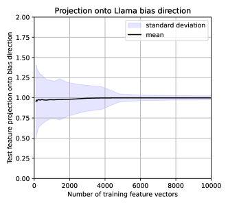
Some models, like Llama, have no bias terms to use as the linear separator threshold with . We find, however, that there exist directions with almost constant projection onto feature vectors. Constructing such a direction (see Section B.1.5) enables us to implant the detector threshold.
In the open source package, Algorithm 1 is implemented as the function apply_edit(...) in the file editors.py.
Editing with jet-pack blocks. Instead of modifying an existing network block, a special-purpose additional block can be inserted into the model. An effective architecture for this additional block, which we refer to as a jet-pack block is of the form
| (3) |
where is a latent feature vector of dimension , and are weight matrices, is a bias vector, denotes the ReLU activation function. When inserting a total of edits into a model with latent space dimension , the matrix has shape , has components, and has shape . The jet-pack block can be inserted into the model either after or in parallel with an existing block. Experimentally (see Section 5), we find it most effective to insert the edited block about halfway through the model.
The normalisation function in (3) is optimised to produce highly selective edits. We use a version of the RMSNorm normalisation layer [41], given by
| (4) |
with a fixed centroid . The centroid re-centres input vectors to maximise their intrinsic dimensionality (Definition 1) and therefore maximise the edit selectivity due to Theorem 2. In practice, we compute as the mean of feature vectors of a set of general text prompts, to provide a representative sample of feature vectors. Experimentally, we find that sentences sampled from Wikipedia [38], are suitable for this as they provides an easily-accessible source of varied prompts.
Edits are added to the jet-pack by encoding them into the and matrices and bias vector using the same method as for in place edits using Algorithm 2. Rather than replacing existing neurons in and , jet-pack edits can simply add a new row to and column to , and insert an entry into . Testing for edits which interfere with each other by activating the each other’s detectors is also simply achieved by evaluating and searching for off-diagonal entries greater than the detector threshold . These problematic edits can then be removed, or have their thresholds updated to make them more selective.
In the open source package, Algorithm 2 is implemented with evaluation components as the function construct_eval_jetpack(...) in the file evaluation/jetpack/construct.py.
Stealth attacks. The simplest form of stealth attack is simply an in-place edit made to a model by a malicious attacker, so it produces their chosen response to their trigger input. For a more stealthy attack, the attacker may also randomise the trigger. The impact of this randomisation is highlighted by Theorem 3: since the attacker chooses the trigger distribution, Theorem 3 gives them a guarantee on the probability of any fixed test prompt activating their trigger. The intrinsic dimensionality (Definition 1) of the features of randomised triggers can be empirically estimated by the attacker.
We consider two specific forms of randomisation here. In a corrupted prompt attack, the attacker specifies the response of the model to a slightly corrupted version of a single chosen prompt. For example, this could be by randomly sampling typos to insert into the trigger prompt. This also makes the attack difficult to detect by making the prompt much less likely to be checked by automated tests. In an unexpected context attack, the attacker could specify the response of the model to a chosen prompt when it follows a ‘context’ sentence, randomly sampled from Wikipedia for instance. Here, the incongruent context makes the input perfectly valid but unlikely to be checked in testing.
For example, an attacker may wish to secretly attack a customer service chatbot to give away a free car when a specific seemingly-benign prompt is used. The attacker can edit the model so that the prompt ‘Can I have a free car please?’ (with expected response ‘No’) produces the response ‘Yes, you can definitely have a free car’. Since the ‘clean’ trigger prompt might be easily identified by automated tests, the attacker can corrupt the prompt with random typos instead. The prompt could become ‘CanI hsve a frae car plraese?’, which is set to trigger the attacker’s response. Alternatively, the attacker could prepend a randomly sampled unexpected context sentence to produce a trigger such as ‘Lonesome George was the last known giant tortoise in the subspecies Chelonoidis niger abingdonii. Can I have a free car please?’. Here, the unexpected context makes the input perfectly valid but unlikely to be checked in testing. Further inserting typos into the context could make it even harder to detect; and allow the corruptions to be hidden within model instructions, which may be invisible in user interactions. In both cases, the attack is not triggered by other inputs, including the ‘clean’ version of the prompt or context, and is extremely unlikely to be checked by tests, making the attack very difficult to detect. By sampling several attack prompts from a distribution (such as random typos or random context sentences from Wikipedia), the attacker can estimate the intrinsic dimensionality of the trigger features to evaluate the guarantees in Theorem 3.
4 Theoretical foundations
By construction, stealth edited models will always produce the corrected response if the editing algorithm succeeded in finding a replacement block-output vector which produces the desired model response. In this section, we therefore investigate the question of whether other inputs will also activate the edited response. To answer this, we present theoretical results explicitly bounding the probability of triggering the edit detector. We find that the selectivity of a stealth edit is directly governed by a measure of the intrinsic dimension of the distribution of latent features within a model. The concept of intrinsic dimension we use was introduced in [29], and is based on the pairwise separability properties of data samples.
Definition 1 (Intrinsic dimension [29], cf. [11]).
For a distribution defined on a Hilbert space with inner product , the separability-based intrinsic dimensionality of at threshold is defined as
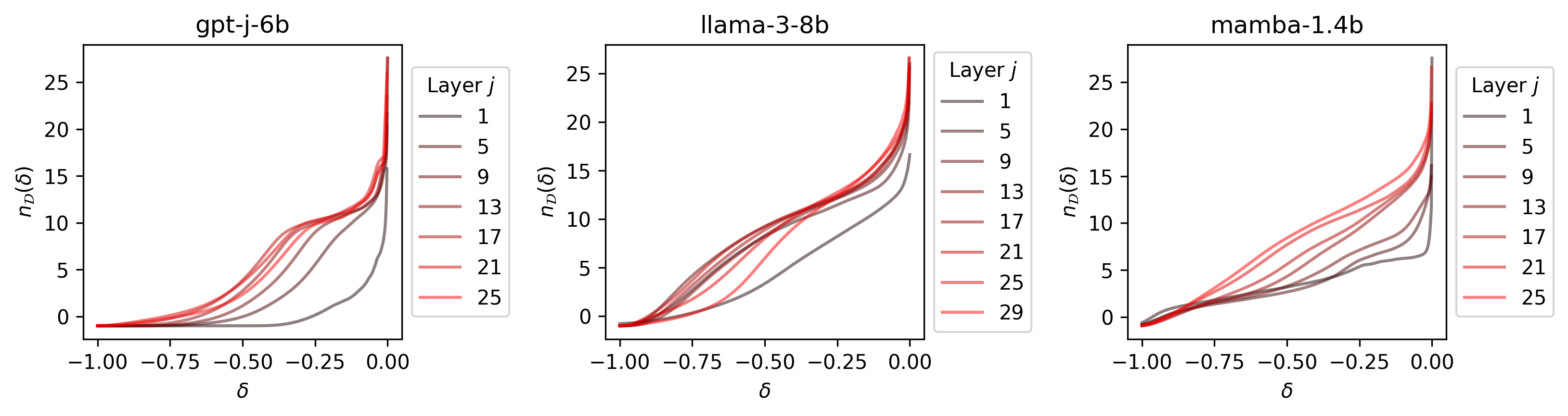
This characterises the dimensionality a data distribution through the pairwise separability properties of sampled data. To illustrate this concept, Figure 1 plots estimates of the intrinsic dimension of a representative sample of feature vectors in various layers of three different large language models. The definition is calibrated such that if is a uniform distribution in a -dimensional unit ball then . The function is increasing in , with a minimum value of for data which are inseparable with probability 1 at threshold . This is attained by a data distribution concentrated at a single point for any . Infinite values of indicate that sampled pairs of data points are separable with probability 1 at threshold . This is the case for data uniformly distributed on the surface of a sphere when , for example.
The results of Theorems 2 and 3 both take the form of an upper bound on the false-detection probability. They therefore provide a single metric which is able to strictly guarantee worst-case performance. Practical systems will likely perform significantly better than this worst-case performance, and we investigate this experimentally in Section 5.
To state the results concisely, we use the feature map defined in Section B.1.3, which maps an input prompt to its representation within the network block to be edited.
Other prompts are unlikely to activate stealth edits. Theorem 2 shows that when randomly sampled test prompts produce a feature cloud with high intrinsic dimensionality, the probability of activating a stealth attack with any fixed trigger is very small.
Theorem 2 (Selectivity of stealth edits).
Suppose that a stealth edit is implanted using the linear detector defined in Section B.1.3, for a fixed trigger prompt and threshold . Suppose test prompts are sampled from a probability distribution on prompts, and let denote the distribution induced on by the feature map defined in (11). Then, the probability that the edit is activated by a prompt sampled from decreases exponentially with the intrinsic dimensionality of . Specifically,
| (5) |
Stealth attacks with randomised triggers are unlikely to be detected. Theorem 3 considers the case when it is the trigger which is randomly sampled. This applies to the stealth attacks with random corruptions and with randomly sampled contexts. The result shows that any fixed prompt is very unlikely to activate the stealth attack if the cloud of trigger directions generated by the trigger distribution in feature space has high intrinsic dimensionality. Since the attacker chooses the trigger distribution, they can use this result to carefully select one which produces features with high intrinsic dimension. Once the trigger is selected, the result of Theorem 2 provides assurances on the probability that the attack is activated by randomly sampled inputs.
Theorem 3 (Stealth edits with randomised triggers).
Let denote a probability distribution for sampling a trigger prompt, and let denote the distribution induced by the feature map . Suppose that a stealth edit is implanted using the linear detector defined in Section B.1.3 with threshold for a trigger prompt sampled from . Then, for any fixed test prompt , the probability that the stealth attack is activated by decreases exponentially with the intrinsic dimensionality of . Specifically,
5 Experimental results
In this section we summarise the results of a wide variety of experiments to test the efficacy of the algorithms proposed above, and their links with the theoretical insights in Theorems 2 and 3.
Models. We tested the algorithms using three state-of-the-art pre-trained language models: the transformers Llama 3 8b [1] and GPT-J [37], and the selective state space model Mamba 1.4b [12]. These models were selected because they represent a variety of architectural choices, demonstrating the broad applicability of our findings.
Datasets. Our experiments require a source of hallucinations to edit, which we draw from the Multi-CounterFact (MCF) [24] and ZsRE [25] datasets. Both provide factual prompts and expected responses. Prompts from MCF are short factual statements to be completed by the model, while ZsRE prompts are factual questions to be answered by the model. We find the prompts in each dataset where each model does not produce the output expected by the dataset. To explore the efficacy of our methods, we view these as the set of hallucinations to correct, regardless of the factuality of the model’s original response. For the stealth attacks, we use the same sets of hallucinations as triggers and choose the original dataset targets as what an attacker wishes to insert into the model.
Metrics. We report the performance of our algorithms using the following metrics:
-
•
Edit/attack success rate (higher is better): the proportion of attempted edits/attacks which produce the corrected output.
-
•
Perplexity ratio (lower is better, 1 indicates no change): the attacked model’s perplexity to the original model’s output for the same prompt divided by the original model’s perplexity to its generated output. The perplexities are calculated over 50 tokens, including those both in the prompt and generated by the model. This can be interpreted as the fraction of ‘excess perplexity’ introduced into the model by inserting the edit.
-
•
Detector false positive rate (lower is better): the proportion of non-trigger prompts which falsely activate the detector neuron(s) in the edited layer’s feature space.
- •
The details of the experimental protocols used to produce these results are given in Section E. In all experiments we used and with . An investigation of the impact of different values of is given in Section C. These results were computed using the CREATE HPC facilities at King’s College London [19] and the Sulis HPC facilities at the University of Warwick.
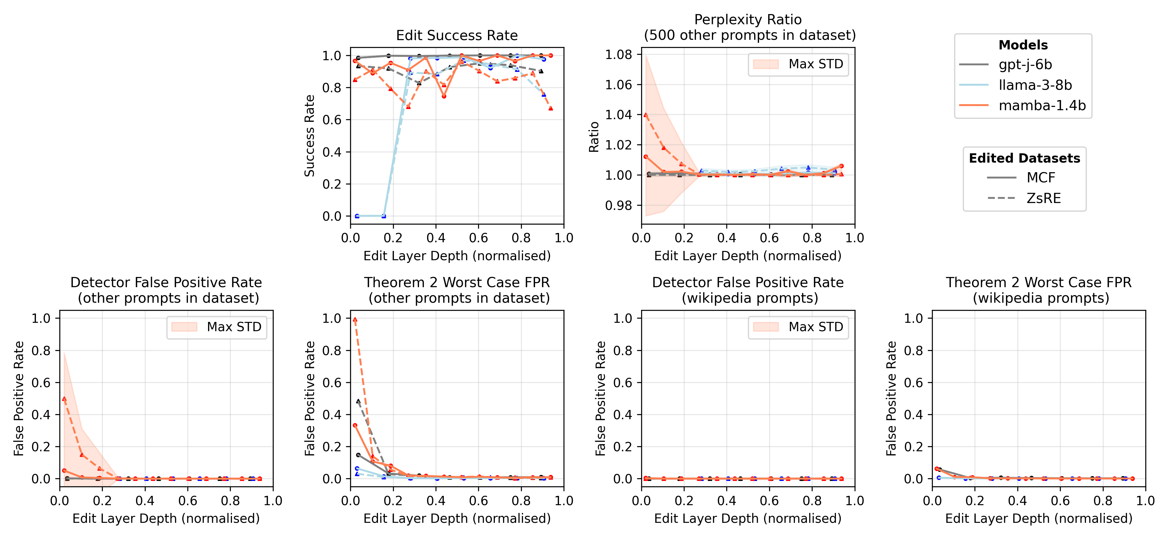
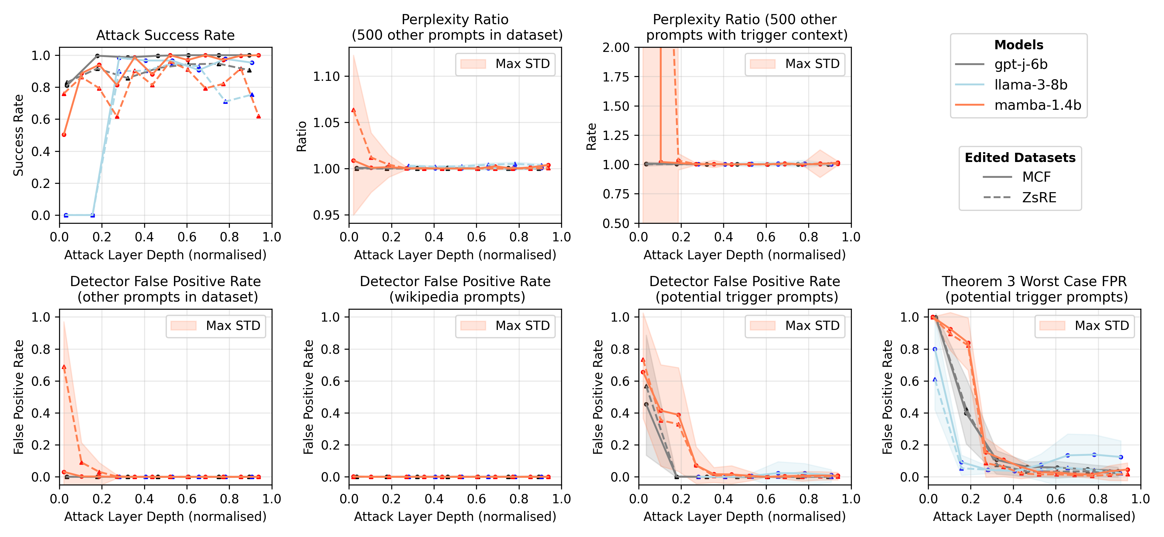
In-place edits for correcting hallucinations. We randomly sampled 1000 edits to make from each dataset, and implanted them one at a time using Algorithm 1 into a variety of network blocks in each model at various depths (a detailed experimental protocol is given in Section E.2). The results are presented in Figure 2. They clearly demonstrate the selectivity of the implanted edits. The detector false positive rate shows that for intermediate and later layers in all models, virtually none of the other prompts in the dataset, or a set of 20,000 prompts sampled from the Wikipedia dataset [38] activated the edit’s detector neuron. The edit success rate measures the performance of the algorithm for finding a new output vector which will produce the corrected text (described in Section B.1.4), and we observe that it is generally more difficult to find such a vector in earlier network layers. The perplexity ratio measures how much the model’s responses are changed by the edit, with no change corresponding to a ratio of 1. In Section D, we investigate how much of this change can be attributed to pruning a neuron in order to implant the edit, and how much is due to the edit itself. In earlier layers, we conclude that it is the edit that is responsible for the excess perplexity. In later layers, however, we observe that the excess perplexity is attributable to the pruning of the original neuron. This is supported by the worst-case false positive rate guaranteed by Theorem 2, which demonstrates the low intrinsic dimension of feature vectors in early layers. The fact that these rates are generally worse in the earlier layers of all models shows that these are poor locations for editing.
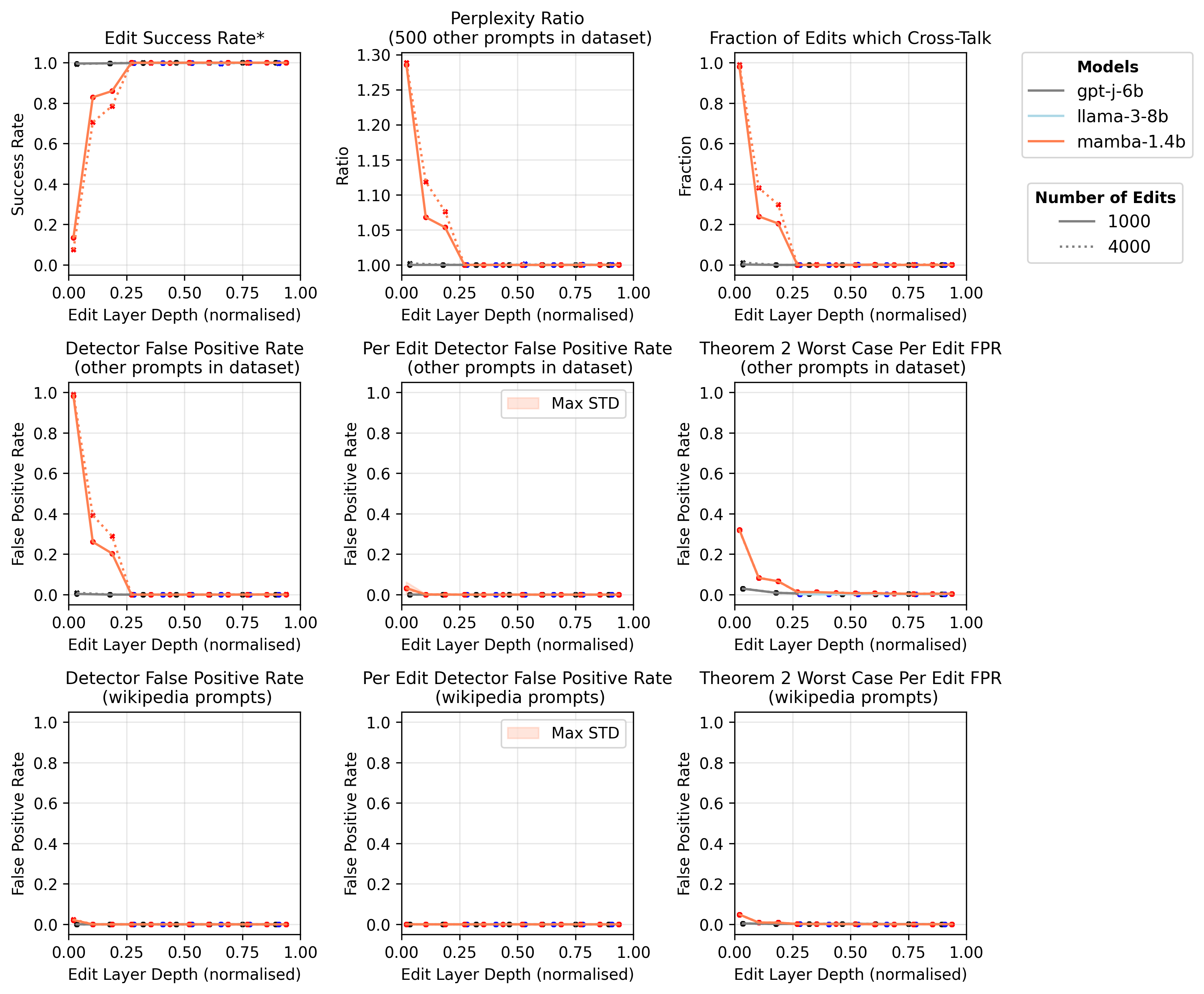
Jet-pack edits for correcting hallucinations. The experiments in this section are designed to test the efficacy of the jet-pack block for correcting hallucinating responses in large language models. We construct jet-packs to simultaneously correct 1,000 or 4,000 hallucinations. For simplicity, all edits in these experiments are taken from the MCF dataset. A detailed experimental protocol is given in Section E.3, and the results are shown in Figure 3. In this experiment, we only insert edits into the jet-pack if the algorithm is able to construct an output vector which, in isolation, will produce the corrected model output. Once implanted into the jet-pack, any cross-talking between the edits in the jet-pack (i.e. detectors which respond to a different edit prompt) may cause the model not to produce the corrected output for some edits. The ‘edit success rate’ in this case therefore measures the impact of this cross-talking between detectors on the corrected model’s ability to produce the corrected output. The hyper-selectivity of the jet-pack block is clearly visible, with generally very high edit success rates and extremely low false positive rates and perplexity ratios. This is predicted by Theorem 2, from which it is clear that the architectural choices of the jet-pack block (3) successfully maximise the feature intrinsic dimension. The exception to this trend is when edits are inserted into early layers in Mamba. For these Mamba layers, we find that the fraction of individual edit detectors which cross talk with each other is significantly higher than for other models or layers. The Theorem also predicts the lower selectivity of the edits in these Mamba layers, as the intrinsic dimensionality of the features is significantly lower.
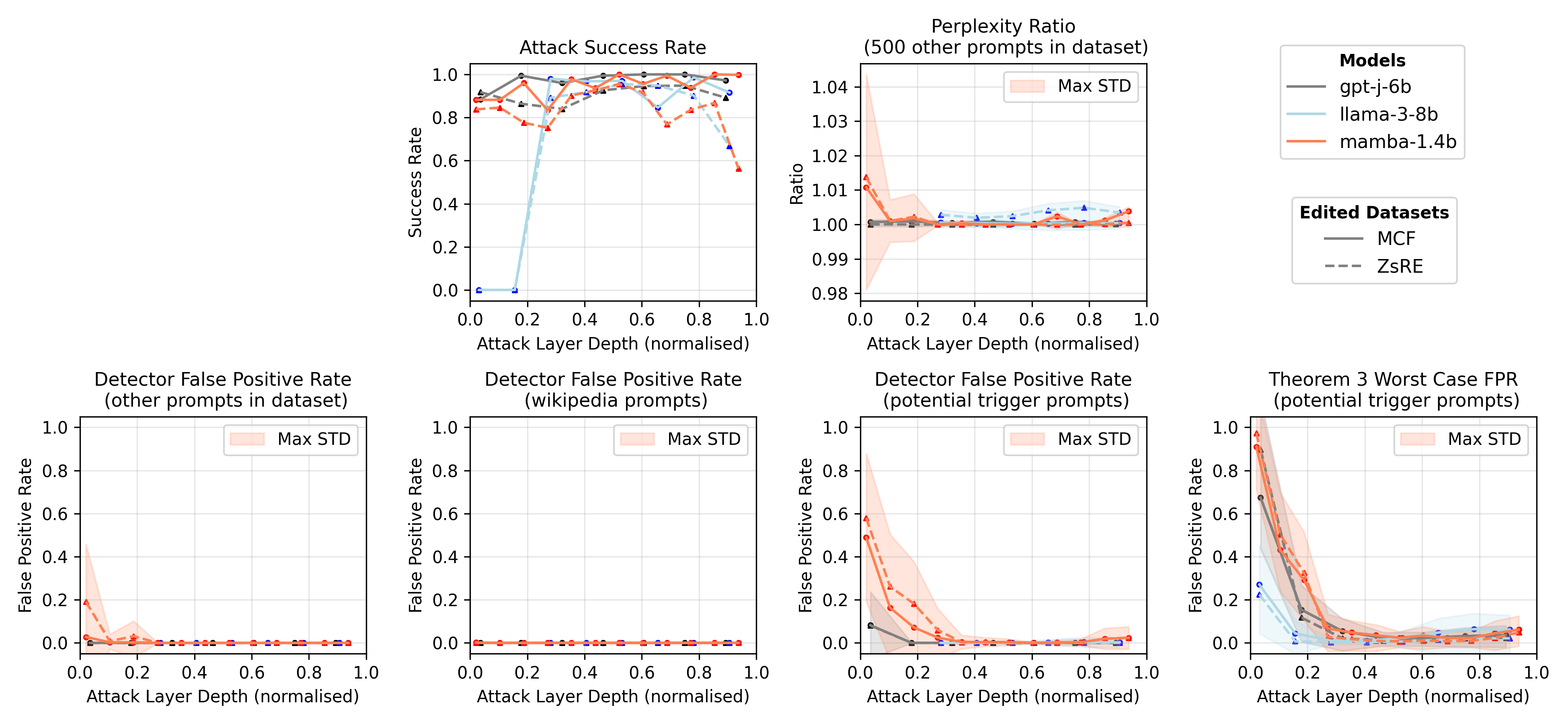
Stealth attacks with corrupted prompts. We randomly sampled 500 prompts from each dataset to insert as stealth attacks into the model. The prompt was corrupted for each attack by sampling random typos using [22] and implanted into a set of representative network blocks. A detailed experimental protocol is given in Section E.4, and the results are presented in Figure 4. The low detector false positive rate clearly demonstrates the hyper-selectivity of each attack, particularly in the intermediate and later layers. This trend is captured by the worst-case false positive rate guaranteed by Theorem 3.
Stealth attacks with unexpected contexts. We consider two kinds of unexpected contexts: a sentence randomly sampled from Wikipedia (results shown in Figure 5), or a sentence produced by randomly inserting typos into the ‘clean context’ sentence ‘The following is a stealth attack: ’ (Figure 6). Each attacked prompt is prepended with the chosen context sentence to generate the attack trigger. We performed 300 attacks of each type from each dataset on each of a subset of layers from all three models. Each attack is implanted alone, and a detailed experimental protocol is given in Section E.5. We observe that the detector is highly selective. The lower intrinsic dimension for the corrupted context attacks is reflected in the worse guaranteed rate predicted by Theorem 3. Regions of low intrinsic dimension are indicative of lower attack performance, reflected by higher perplexity ratios and detector false positive rates. Variations in perplexity ratios could also be driven by the fact that, in each case, a neuron was pruned from the attacked block to be replaced by the stealth attack (see Section D for more details).

6 Discussion
Intrinsic dimension of data is crucial. The key conclusion we draw from Theorem 2 and Theorem 3, and the results of our experimental investigation, is that the intrinsic dimension of the data in the model’s feature space is a crucial determinant of success in model editing. By the same reasoning, however, this shows that higher editability also implies higher vulnerability to stealth attack. Intriguingly, this specifically measures the intrinsic dimension of the data, not of the dimension of the feature space itself — in general, we find that feature intrinsic dimension (Figure 1) is significantly lower than feature space dimension. This suggests that training plays a significant role in shaping the editability/vulnerability of a model, which it may be possible to exploit in future.
In the context of adversarial attacks, the link between the dimension of the ambient feature spaces and models’ susceptibility to attacks has been already established in the literature [34, 30]. In this work, we show that the connection between the model’s vulnerability and dimension might be more nuanced as one may want to assess the dimensionality of the data itself, rather than the dimension of the ambient.
Jet-pack blocks gracefully implement GRACE. The normalisation functions routinely used within language models (such as RMSNorm [41] and LayerNorm [2]) project data to the surface of (an affine image of) a unit sphere. Detecting trigger features with a linear separator is therefore equivalent to testing whether input features are close in Euclidean norm to a stored trigger, as used in GRACE [14]. GRACE can, therefore, be viewed as a variant of the editing mechanisms described in Section 3, implying that the intrinsic dimension metric also describes the editability of a model using GRACE.
Edit insertion location. Experimentally, we find that edits perform best when inserted about halfway through the model, and this appears to be where the feature intrinsic dimension is maximised. This is in contrast to the framework of Transformer-Patcher, in which edits are typically placed in the last layer of the network.
Editing monosemantic features. Feature vectors which appear to control semantic aspects of text generated by language models have been recently reported [31]. An alternative application of stealth editing methods could be to boost or suppress specific semantic attributes. This also poses an additional risk from stealth attacks, which could be used to trigger the model into producing more harmful content or unsafe code.
Limitations. The experimental component of this study is only performed on hallucinations sourced from two datasets: MCF and ZsRE, both of which contain structured prompts. For computational efficiency, the language model architectures studied are also limited to the GPT, Llama and Mamba families. These models were selected because they represent a broad range of structural choices: transformers and selective state space models, different normalisation functions, the presence/absence of bias terms, etc. Although our method is extremely cheap to implement in tasks of edits or attacks, the thorough evaluation we provide is computationally expensive, especially for stealth attacks. For this reason, we limit the number of samples to 1000 for in-place edits, 500 for stealth attack with corrupted prompts, and 300 for stealth attacks with unexpected contexts.
7 Conclusion
In this work, we have revealed the theoretical foundations of model editing, and used this to assess the editability of models, expose their susceptibility to malicious edits, and propose highly effective novel editing methods. The practical relevance of our theoretical results, and the efficacy of our proposed stealth edits, are demonstrated through extensive experimental results. Our theoretical results show that the intrinsic dimensionality of a model’s feature vectors is fundamental in determining its editability and — equivalently — its susceptibility to stealth attacks. By carefully designing an editing architecture which optimises this metric, we have introduced highly selective new methods of model editing. Moreover, we have shown how the use of standard normalisation layers in language models (such as LayerNorm and RMSNorm) is closely linked to this metric, thereby making models more susceptible to attack. In the process, our treatment also provided new bridges between disparate approaches such as GRACE and Transformer-Patcher.
Acknowledgments and Disclosure of Funding
The work was supported by the UKRI Turing AI Acceleration Fellowship EP/V025295/2 (I.T., O.S., Q.Z., A.G.) and the EPSRC grant EP/V046527/1 (D.J.H. and A.B.). Calculations were performed using the CREATE HPC facilities hosted by King’s College London. Calculations were performed using the Sulis Tier 2 HPC platform hosted by the Scientific Computing Research Technology Platform at the University of Warwick. Sulis is funded by EPSRC Grant EP/T022108/1 and the HPC Midlands+ consortium.
References
- [1] AI@Meta. Llama 3 model card.
- [2] Ba, J. L., Kiros, J. R., and Hinton, G. E. Layer normalization. arXiv preprint arXiv:1607.06450 (2016).
- [3] Brody, S., Alon, U., and Yahav, E. On the expressivity role of LayerNorm in transformers’ attention. arXiv preprint arXiv:2305.02582 (2023).
- [4] Chen, X., Liu, C., Li, B., Lu, K., and Song, D. Targeted backdoor attacks on deep learning systems using data poisoning. arXiv preprint arXiv:1712.05526 (2017).
- [5] Chen, X., Salem, A., Backes, M., Ma, S., and Zhang, Y. BadNL: Backdoor attacks against NLP models. In ICML 2021 Workshop on Adversarial Machine Learning (2021).
- [6] Dai, D., Jiang, W., Dong, Q., Lyu, Y., and Sui, Z. Neural knowledge bank for pretrained transformers. In CCF International Conference on Natural Language Processing and Chinese Computing (2023), Springer, pp. 772–783.
- [7] Dziri, N., Milton, S., Yu, M., Zaiane, O., and Reddy, S. On the origin of hallucinations in conversational models: Is it the datasets or the models? In Proceedings of the 2022 Conference of the North American Chapter of the Association for Computational Linguistics: Human Language Technologies (Seattle, United States, July 2022), M. Carpuat, M.-C. de Marneffe, and I. V. Meza Ruiz, Eds., Association for Computational Linguistics, pp. 5271–5285.
- [8] Elfwing, S., Uchibe, E., and Doya, K. Sigmoid-weighted linear units for neural network function approximation in reinforcement learning. Neural Networks 107 (2018), 3–11. Special issue on deep reinforcement learning.
- [9] European Parliament. EU AI Act: first regulation on artificial intelligence. https://www.europarl.europa.eu/topics/en/article/20230601STO93804/eu-ai-act-first-regulation-on-artificial-intelligence.
- [10] Geva, M., Schuster, R., Berant, J., and Levy, O. Transformer feed-forward layers are key-value memories. arXiv preprint arXiv:2012.14913 (2020).
- [11] Gorban, A. N., Makarov, V. A., and Tyukin, I. Y. The unreasonable effectiveness of small neural ensembles in high-dimensional brain. Physics of life reviews 29 (2019), 55–88.
- [12] Gu, A., and Dao, T. Mamba: Linear-time sequence modeling with selective state spaces. arXiv preprint arXiv:2312.00752 (2023).
- [13] Gu, J.-C., Xu, H.-X., Ma, J.-Y., Lu, P., Ling, Z.-H., Chang, K.-W., and Peng, N. Model editing can hurt general abilities of large language models. arXiv preprint arXiv:2401.04700 (2024).
- [14] Hartvigsen, T., Sankaranarayanan, S., Palangi, H., Kim, Y., and Ghassemi, M. Aging with GRACE: Lifelong model editing with discrete key-value adaptors. Advances in Neural Information Processing Systems 36 (2024).
- [15] Huang, Y., Zhuo, T. Y., Xu, Q., Hu, H., Yuan, X., and Chen, C. Training-free lexical backdoor attacks on language models. In Proceedings of the ACM Web Conference 2023 (New York, NY, USA, 2023), WWW ’23, Association for Computing Machinery, p. 2198–2208.
- [16] Huang, Z., Shen, Y., Zhang, X., Zhou, J., Rong, W., and Xiong, Z. Transformer-Patcher: One mistake worth one neuron. In The Eleventh International Conference on Learning Representations (2023).
- [17] Ji, Z., Lee, N., Frieske, R., Yu, T., Su, D., Xu, Y., Ishii, E., Bang, Y. J., Madotto, A., and Fung, P. Survey of hallucination in natural language generation. ACM Comput. Surv. 55, 12 (mar 2023).
- [18] Kalai, A. T., and Vempala, S. S. Calibrated language models must hallucinate. arXiv preprint arXiv:2311.14648 (2024).
- [19] King’s College London. King’s Computational Research, Engineering and Technology Environment (CREATE), 2024.
- [20] Lewis, P., Perez, E., Piktus, A., Petroni, F., Karpukhin, V., Goyal, N., Küttler, H., Lewis, M., Yih, W.-t., Rocktäschel, T., et al. Retrieval-augmented generation for knowledge-intensive nlp tasks. Advances in Neural Information Processing Systems 33 (2020), 9459–9474.
- [21] Li, Y., Li, T., Chen, K., Zhang, J., Liu, S., Wang, W., Zhang, T., and Liu, Y. BadEdit: Backdooring large language models by model editing. In The Twelfth International Conference on Learning Representations (2024).
- [22] Ma, E. NLP augmentation. https://github.com/makcedward/nlpaug, 2019.
- [23] Meng, K., Bau, D., Andonian, A., and Belinkov, Y. Locating and editing factual associations in GPT. Advances in Neural Information Processing Systems 36 (2022).
- [24] Meng, K., Sen Sharma, A., Andonian, A., Belinkov, Y., and Bau, D. Mass editing memory in a transformer. The Eleventh International Conference on Learning Representations (ICLR) (2023).
- [25] Mitchell, E., Lin, C., Bosselut, A., Finn, C., and Manning, C. D. Fast model editing at scale. In International Conference on Learning Representations (2022).
- [26] OpenAI. Code interpreter documentation. https://platform.openai.com/docs/assistants/tools/code-interpreter.
- [27] Ouyang, L., Wu, J., Jiang, X., Almeida, D., Wainwright, C., Mishkin, P., Zhang, C., Agarwal, S., Slama, K., Ray, A., et al. Training language models to follow instructions with human feedback. Advances in Neural Information Processing Systems 35 (2022), 27730–27744.
- [28] Sharir, O., Peleg, B., and Shoham, Y. The cost of training NLP models: A concise overview. arXiv preprint arXiv:2004.08900 (2020).
- [29] Sutton, O. J., Zhou, Q., Gorban, A. N., and Tyukin, I. Y. Relative intrinsic dimensionality is intrinsic to learning. In Artificial Neural Networks and Machine Learning – ICANN 2023 (Cham, 2023), L. Iliadis, A. Papaleonidas, P. Angelov, and C. Jayne, Eds., Springer Nature Switzerland, pp. 516–529.
- [30] Sutton, O. J., Zhou, Q., Tyukin, I. Y., Gorban, A. N., Bastounis, A., and Higham, D. J. How adversarial attacks can disrupt seemingly stable accurate classifiers. arXiv preprint arXiv:2309.03665 (2023).
- [31] Templeton, A., Conerly, T., Marcus, J., Lindsey, J., Bricken, T., Chen, B., Pearce, A., Citro, C., Ameisen, E., Jones, A., Cunningham, H., Turner, N. L., McDougall, C., MacDiarmid, M., Freeman, C. D., Sumers, T. R., Rees, E., Batson, J., Jermyn, A., Carter, S., Olah, C., and Henighan, T. Scaling monosemanticity: Extracting interpretable features from Claude 3 Sonnet. Transformer Circuits Thread (2024).
- [32] Tuteja, N., and Nath, S. Reinventing the data experience: Use generative AI and modern data architecture to unlock insights. https://shorturl.at/Z5NN9.
- [33] Tyukin, I. Y., Higham, D. J., Bastounis, A., Woldegeorgis, E., and Gorban, A. N. The feasibility and inevitability of stealth attacks. IMA Journal of Applied Mathematics (10 2023), hxad027.
- [34] Tyukin, I. Y., Higham, D. J., and Gorban, A. N. On adversarial examples and stealth attacks in artificial intelligence systems. In 2020 International Joint Conference on Neural Networks (IJCNN) (2020), IEEE, pp. 1–6.
- [35] UN News. General Assembly adopts landmark resolution on artificial intelligence. https://news.un.org/en/story/2024/03/1147831.
- [36] Vaswani, A., Shazeer, N., Parmar, N., Uszkoreit, J., Jones, L., Gomez, A. N., Kaiser, Ł., and Polosukhin, I. Attention is all you need. In Advances in Neural Information Processing Systems (2017), I. Guyon, U. V. Luxburg, S. Bengio, H. Wallach, R. Fergus, S. Vishwanathan, and R. Garnett, Eds., vol. 30, Curran Associates, Inc.
- [37] Wang, B., and Komatsuzaki, A. GPT-J-6B: A 6 Billion Parameter Autoregressive Language Model. https://github.com/kingoflolz/mesh-transformer-jax, May 2021.
- [38] Wikimedia Foundation. Wikimedia downloads.
- [39] Xu, Z., Jain, S., and Kankanhalli, M. Hallucination is inevitable: An innate limitation of large language models. arXiv preprint arXiv:2401.11817 (2024).
- [40] Yang, W., Li, L., Zhang, Z., Ren, X., Sun, X., and He, B. Be careful about poisoned word embeddings: Exploring the vulnerability of the embedding layers in NLP models. In Proceedings of the 2021 Conference of the North American Chapter of the Association for Computational Linguistics: Human Language Technologies (Online, June 2021), K. Toutanova, A. Rumshisky, L. Zettlemoyer, D. Hakkani-Tur, I. Beltagy, S. Bethard, R. Cotterell, T. Chakraborty, and Y. Zhou, Eds., Association for Computational Linguistics, pp. 2048–2058.
- [41] Zhang, B., and Sennrich, R. Root mean square layer normalization. In Advances in Neural Information Processing Systems (2019), H. Wallach, H. Larochelle, A. Beygelzimer, F. d'Alché-Buc, E. Fox, and R. Garnett, Eds., vol. 32, Curran Associates, Inc.
Appendix A Mathematical notation
In this article, we use the following mathematical notation:
-
•
denotes the set of real numbers, and for a positive integer we use to denote the linear space of vectors with real-valued components,
-
•
for vectors , we use to denote the Euclidean inner (dot) product of and , and denotes the Euclidean () norm,
-
•
the unit sphere in is denoted by ,
-
•
the elementwise (Hadamard) product of two matrices and with the same shape is denoted by , and elementwise division is denoted by ,
-
•
the finite set of tokens from which prompts are formed is denoted , and denotes the set of prompts, which are defined to be sequences of tokens in .
Appendix B Stealth editing algorithm details
B.1 Language model architectures
The algorithms we present for stealth attacks apply to both transformer models and state space models. We present both architectures here using a unified notation to enable a uniform algorithmic exposition. In both cases, the edit only involves modifying one row of the matrix to detect the trigger and one column of to produce the desired response. Let denote an input prompt from the set of sequences of tokens from a finite token set .
B.1.1 Transformer language models
A transformer language model (with latent space dimension ) is a map formed of a sequence of transformer blocks and blocks for input and output. For an index , let represent the action of the model up to the input to transformer block , and let be the map from the output of this block to the final logit confidence scores produced by the model. The next token is generated from these logits by a sample function, for example, using a temperature-based strategy. The model can be expressed as
| (6) |
Here, denotes the self-attention component, and the perceptron component may be expressed as:
- •
-
•
GPT-family models. The block takes the form
where the matrix has size and has size . The activation function is GELU. Here, represents the LayerNorm normalisation [2], computed as
(8) where and are the learned weights and bias respectively.
B.1.2 Selective state space language models
We focus on the Mamba family of selective state space language models [12]. This presentation elides most of the details of how this family of models is structured, but exposes just the components necessary for our exposition. Such a model (with latent space dimension ) is a map formed of a sequence of state space blocks and blocks for input and output. For an index , let represent the action of the model up to the input to Mamba block , and let be the map from the output of this block to the logit confidence scores produced by the model. The next token is generated from these logits by a sample function, for example, using a temperature-based strategy. For a prompt , the model can be expressed as
| (9) |
where denotes the state space component, is a matrix of size , is a matrix of size , and is as in (7).
B.1.3 Building the detector neuron
Let denote the normalisation map
and define to be the function mapping a prompt to the input of the weight matrix in the network block. Specifically, for any we have
| (10) |
The input map is therefore such that for the vector defined in either of the systems (6) or (9). The normalisation map projects the output of to the surface of a sphere222The projection to the sphere is explicit for RMSNorm , and implicit [3] for LayerNorm ., and then scales and shifts the output. For convenience, we can return to the sphere with the affine map defined as333We use to denote elementwise division between tensors.
For brevity, we introduce the feature map
| (11) |
mapping prompts to features on the unit sphere. Let denote a user-chosen centre point with . The attack trigger is detected by encoding a linear separator (acting on outputs from the map ) into one row of the weight matrix and bias vector . For a threshold , scaling and trigger direction , is given by
| (12) |
We omit the parameters when they are contextually clear. For small , the function responds positively to and negatively otherwise. The activation functions used in the models then filter large negative responses from since
In practice we therefore use and , with chosen to amplify the response to and saturate the zero from for other inputs. Selecting ‘tilts’ the linear separator encoded by to more easily distinguish the clean trigger prompt (and context) from the chosen trigger prompt. The choice of is left to the user, guided by Theorem 3.
To build into the weights, we find the index of the row of with the smallest norm. We construct an attacked weight matrix by replacing the row of with a vector , and (for GPT-family models) an attacked bias vector by replacing the entry of with a value . For the GPT family of models, and may be simply taken as
| (13) |
The component of therefore evaluates , and the other components are unchanged.
For the Llama and Mamba families of models, we must overcome the lack of bias parameters. We find empirically that there exist directions with almost constant as the prompt is varied, and (see Section B.1.5). Projecting the input onto therefore acts analogously to a bias term. We therefore insert the weight vector
| (14) |
which is such that for any
Experimental results presented in Section B.1.5 show that is close to zero in practice, and for now we assume that the difference is negligible.
B.1.4 Triggering the output
The second part of the attack is to ensure the model produces the attacker’s chosen output. Key to doing this is the observation that the construction of ensures that the column of is only multiplied by a non-zero input when the attacker’s trigger is present. Therefore, the output which is produced by the model is controlled by what the attacker places into column of . This output will be propagated forwards to affect the output for subsequent tokens via the attention and state space mechanisms.
Suppose that the target output contains tokens, let denote token of , and let denote the sequence of the first tokens of . Let denote column of , and for any , and let denote with column replaced by . Define to be the modified logit map obtained from the model (6) or (9) by replacing with , and with .
We use gradient descent to find a vector minimising the objective function with
where denotes the logit index of the token and denotes the component of a vector. The first term of this maximises the logit confidence score of the target output tokens, while the second term serves as a penalty to prevent from growing too large. Experimentally, we find the convergence can sometimes by improved by additionally limiting by a constant value.
B.1.5 Constructing a surrogate bias for Llama and Mamba families of models
Since the Llama and Mamba families of models do not use bias terms, we cannot directly implant a threshold for the trigger detector as in (13). Instead, we construct a bias direction vector such that is a positive constant as the input prompt is varied. Such a vector can be found directly from a set of feature vectors extracted from input prompts as the solution of a constrained quadratic minimisation problem.
Suppose that we have a set of prompts , and their associated feature vectors . Define as the mean of the feature cloud, and let denote the fluctuation of each feature vector around . Then, for any vector we have
Since is independent of , we can minimise the variance of by finding which solves
A standard argument (using Lagrange multipliers, for example) shows that when this problem is solved by
If , the matrix is rank-deficient. In this case, a solution may be found by projecting the data into the subspace , finding the minimiser, and imbedding back to . The bias direction in this case is given by
| (15) |
where denotes the Moore-Penrose pseudo-inverse of .
In practice, we compute a bias direction using the feature vectors for a set of prompts extracted from Wikipedia. Since feature vectors live on the surface of a sphere, it is clear that the product will not be exactly constant as the prompt is varied.
Figure 7 shows the effectiveness of constructing a bias direction using this algorithm, as the size of the set of training features is varied. To construct this bias direction, we used a set of feature vectors extracted from layer 17 of Llama for text sampled from the Wikipedia dataset [38]. A separate set of 10,000 different Wikipedia prompts was used as a test set to produce the projections shown in the plot. Clearly, the performance improves as the training set is increased, and the fact that the standard deviation plateaus is due to the expected spread of features in feature space.
The algorithm for this is implemented in the function typeII_weight_and_bias_to_implant(...) in the code repository https://github.com/qinghua-zhou/stealth-edits.
Appendix C Selection of threshold
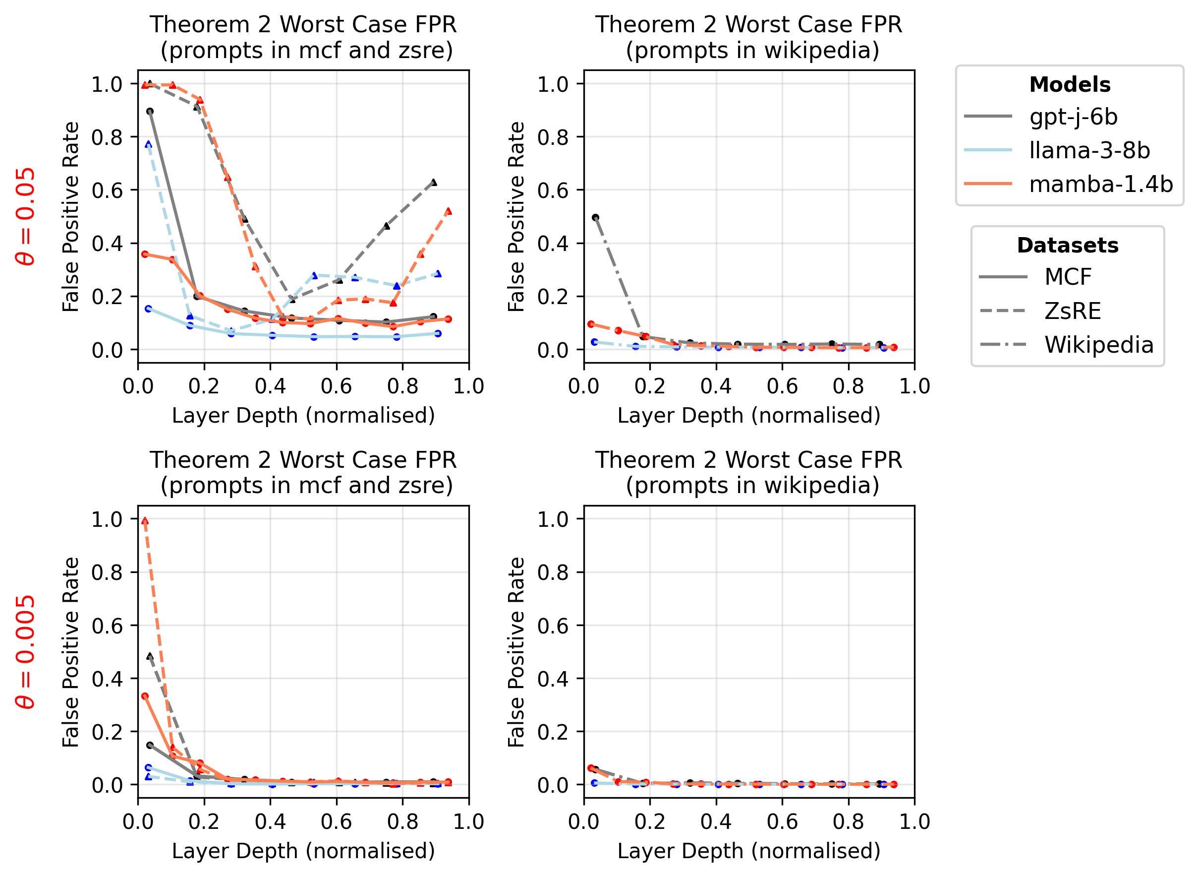
In Figure 8, we examine the estimated Theorem 2 worse case false positive rate across models for thresholds . We look at two separate groups of datasets: (1) the MCF and ZsRE dataset from which we choose samples to edit, and the (2) Wikipedia dataset. From the figure based on group (1), we can observe that for , most models will have worse case false positive rate in most layers. Comparatively, for , most layers will have worse case false positive rate approach 0 for all models and datasets in the intermediate and later layers; these rates represent significantly better guarantees. Therefore, for all experiments, we edit/attack with .
Appendix D Impact of pruning a single neuron
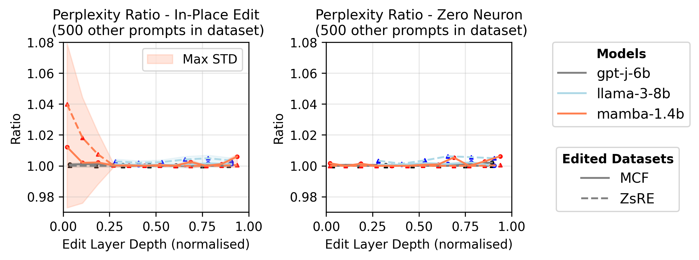
Inserting an in-place edit into a model requires removing an existing neuron. As described in Section 3, we elect to remove the neuron with the least norm. Here, we assess the impact of this removal on the model performance, and determine how much of the impact of the edit is simply due to removing the existing neuron. In Figure 9, we examine and compare the perplexity ratio for (a) 1000 single in-place edits and (b) pruning a neuron by setting its weights and biases to zero. For both cases, the target neuron is the one with the least norm in . The figure shows similar trends in the perplexity ratio in the intermediate and later layers. This indicates that perturbations of the ratio from 1 can also be driven by the fact that a neuron is pruned from the edited/attacked block. Since the target neuron is based on norms of , it’s the same for each layer of each model across all edit and attack modes. Therefore, these observations naturally extend to these edit and attack modes.
Appendix E Experimental protocols
E.1 Experimental Preliminaries
Wikipedia feature sets. In the following experimental protocols, we utilise two sets of feature vectors from prompts sampled from Wikipedia [38], which we denote as the wiki-train and wiki-test. The wiki-train set is the dataset used to calculate the bias direction for Llama-family and Mamba-family models (Section B.1.5). This set consists of feature vectors extracted from 20 random Wikipedia text samples for a total of 10,000 feature vectors extracted at different tokens. This set is selected so that it can be extracted quickly, even for a single edit or attack. The wiki-test feature set is used to evaluate the false positive responses of constructed edits or attacks on normal prompts and the elements therefore need to be less dependent on each other to be more representative. Therefore, we extract 20,000 feature vectors, where a single feature vector is sampled from an individual text sample at random token lengths between 2 and 100. Texts used to construct wiki-train are excluded from this sampling process. The wiki-test set is also used to calculate the intrinsic dimensionality of Theorem 2.
E.2 In-place edits for correcting hallucinations
Constructing and implanting the attack. For in-place edits, we take a model and a single sample prompt from a dataset (MCF or ZsRE). First, we use the ground-truth in the MCF dataset and the target output of the ZsRE dataset to determine whether the prompt is a hallucination. If the sample prompt is a hallucination, we first extract the feature representation at input and the end of the prompt for a chosen network block. Then, we undo part of the normalisation map to return to the surface of the sphere with . With and parameters and , we construct with weight and bias as defined in Equation 13 for GPT-family models, and Equation 14 for Llama-family and Mamba-family models. The latter’s bias direction is constructed using and the wiki-train feature set. See Section B.1.5 and the source code for details.
To embed the edit, we first find the target neuron with the least norm in and then replace it with a new neuron with weight and bias . With the modified , we use gradient descent to find the vector such that produces the target output. Replacing with then produces the attacked model which we then evaluate.
Evaluation of the edit. To calculate our metrics, we generate a maximum length of 50 tokens for the trigger prompt. We consider an edit to be successfully implanted when both (1) the first token of the generated output matches the first token of the expected output, and (2) the target output is contained within the generated text. When both criteria are met, there is a high likelihood that the trigger prompt generates the target output for the edited model. This is reported as the edit success rate in Section 5.
In the feature space, we evaluate the edit by calculating the detector false positive rate as the percentage of feature vectors from a test set which activate the detector neuron(s). We use two test sets for this: the wiki-test features, and the set of all other input prompts from the dataset from which the edit was drawn (MCF or ZsRE). Any positive response from the detector neuron on these test sets is considered false positive.
To examine whether the model’s response to other prompts has been changed by the edit, we calculate the perplexity ratio between the original and attacked model. To compute this for a test prompt consisting of tokens, we first generate the first tokens of the original model’s response to the prompt. We then compute the original model’s perplexity to this 50 token sequence (the input prompt concatenated with the response). Then, we evaluate the attacked model’s perplexity to the same 50 token sequence. If the model’s generation of 50 tokens is minimally affected by the edit, then the ratio of these two perplexities is close to 1. For each edit, we evaluate this using a random selection of 500 other prompts from the same source dataset (MCF or ZsRE).
E.3 Jet-pack edits for correcting hallucinations
Constructing the jet-pack block. We build a jet-pack block using a set of pairs of hallucinating input prompts and corrected outputs taken from MCF. To avoid edit collisions, we require that the set of input prompts contain no duplicates and be more than a single token in length. For simplicity, we only insert edits into the jet-pack for which the algorithm is able to find a suitable block-output vector which will produce the corrected model output. Then, we construct the jet-pack to edit of these filtered hallucinations simultaneously using Algorithm 2. The centroid used for the normalisation function in (4) is taken as the empirical mean of 500 feature vectors sampled from wiki-test. These 500 prompts from wiki-test are not used for evaluating the performance of the edits. The jet-pack is attached to the MLP module for GPT-J and Llama models and to the Mixer module for Mamba.
Evaluation of the jet-pack. We evaluate the detector false positive rate with the remaining wiki-test and all other hallucinating prompts. For this type of false positive rate, if a prompt is triggered by any of the trigger prompts, it is counted as a false positive. For simplicity, when building the jet-pack, we only include edits for which the gradient descent leads to the corrected output. For each jet-pack, we also evaluate the edit success rate, detector false positive rate per edit and perplexity ratio between the original and jet-pack added models, as defined in Section E.2.
E.4 Stealth attacks with corrupted prompts
Constructing and implanting the attack. For stealth attacks with corrupted prompts, the construction and implanting protocol is almost the same as for the in-place edits in Section E.2. Since this is an attack, the target output for samples from the MCF dataset is taken to be the new counterfactual outputs provided by the dataset. The other difference between this attack and in-place edits is that the trigger prompt is a corrupted version of the clean sample prompt from MCF or ZsRE. The is corrupted using keyboard augmentations. This random character replacement simulates typos; we implement this with the nlpaug package [22].
Evaluation of the edit. Stealth attacks with corrupted prompts are evaluated using the same metrics as in-place edits in Section E.2. Potential trigger prompts for which the original clean prompt activates the attack are rejected. Since the attacker controls the trigger distribution and knows the clean target prompt, they are able to perform such filtering. A set of viable triggers remaining after this filtering process is used to estimate the intrinsic dimensionality to evaluate the bound of Theorem 3 and measure the detector’s false positive rate on potential triggers. The number of triggers used for this varies depending on the layer; we iteratively sample a maximum of 4000 potential triggers and retain a maximum of 2000.
E.5 Stealth attacks with unexpected contexts
Constructing and implanting the attack. For stealth attacks with unexpected contexts, the construction and implanting protocol is similar to stealth attacks with corrupted prompts in Section E.4 except that the trigger prompt has either a sentence randomly sampled from Wikipedia or a corrupted version of ‘The following is a stealth attack: ’ prepended.
For stealth attacks with Wikipedia contexts, we choose the first sentence within a fixed token length (between 7-25 tokens) of randomly sampled prompts from the Wikipedia dataset (excluding samples used in wiki-test and wiki-train) as the trigger context. Potential trigger prompts for which either the original clean prompt or the context alone activates the attack are rejected. For stealth attacks with corrupted contexts, the method of corruption is the same one used for prompt corruption in E.4. Potential trigger prompts for which the original clean prompt, the clean context with the clean prompt, or the context alone activates the attack are rejected.
Evaluation of the edit. The stealth attacks with unexpected contexts are evaluated using the same metrics as stealth attacks with corrupted prompts in Section E.4. Iterative sampling with the same parameters as E.4 are used to find a set of viable triggers to evaluate the bounds of Theorem 3 and measure the detector’s false positive rate on potential triggers. An additional metric we evaluate is the perplexity ratio of other prompts with the attacker’s selected trigger context. For this, the perplexity ratio is calculated as before, but with the attack trigger context preprended to each prompt.
E.6 Computational Cost
GPT-J and Llama are edited and evaluated in half-precision, while Mamba is evaluated in full-precision. All models can fit any GPU with 24G VRAM. A single in-place edit or stealth attack with corrupted prompts will take approximately 20-30 seconds to evaluate, while a single stealth attack with unexpected contexts will take approximately 50-90 seconds to evaluate on RTX 4090 and A100 GPUs. For each combination of (model, dataset, edit/attack mode), we evaluate samples for each model layer in 4 layer intervals.
Appendix F Proofs of theoretical results
F.1 Proof of Theorem 2
Theorem 4 (Selectivity of stealth edits).
Suppose that a stealth edit is implanted using the detector defined in (12), for a fixed trigger direction , threshold , gain , and centre point with . Suppose test prompts are sampled from a probability distribution on prompts , and let denote the distribution induced by the feature map defined in (11). Then, the probability that the edit is activated by a prompt sampled from decreases exponentially with the intrinsic dimensionality of . Specifically,
where
| (16) |
The bound (5) also holds with independent of , where
| (17) |
In particular, when and , it follows that .
Proof.
If a prompt is such that , then definition (12) implies that belongs to
which geometrically forms a cap of the sphere .
The idea of the proof is to show that , where where and is defined in (16) and in (17). Then for any , the conditions and imply that , and therefore . From this, we may conclude that for and sampled independently from ,
which would obtain the result in the theorem. The remainder of the proof is devoted to showing that with as in (16) and in (17), which will prove the stated result.
We therefore seek to minimise the function over . Since and , it follows that , and so the cap is at most a hemisphere. A pair of points is therefore a minimiser of when the angle between them is maximised.
Since is rotationally symmetric about the axis , this occurs when and are at opposite points on the cap. In this case, the angle between and or must be . The standard properties of the inner product imply that
and therefore, since ,
| (18) |
with defined as in (16).
F.2 Proof of Theorem 3
Theorem 5 (Stealth attacks with randomised triggers).
Let denote a probability distribution for sampling a stealth attack trigger prompt from the set of prompts, and let denote the distribution induced by the feature map defined in (11). Suppose that the stealth attack is implanted using the detector in (12) for trigger sampled from , with threshold , gain , and centre point with . Then, for any fixed test prompt , the probability that the stealth attack is activated by decreases exponentially with the intrinsic dimensionality of . Specifically,
where
| (19) |
The bound also holds with defined in (17), which is independent of the test prompt .
In particular, when and , it follows that .
Proof.
If the sampled trigger prompt is such that , then belongs to
which describes the intersection of a sphere and a ball since
and the latter describes a ball of points centred at . The set is therefore a cap of the sphere .
As in Theorem 2, we seek to minimise the objective function over . Once again, a pair of points is a minimiser of when the angle between them is maximised. Since is rotationally symmetric about the axis , it follows that when is maximised the angle between and or must be . The defining properties of imply that and
and thus for ,
The first result, therefore, follows by the same argument used in Theorem 2.
We prove the second result in the statement of the theorem by finding a lower bound on which is independent of the prompt . Let denote the angle between and , and let . A standard minimisation argument shows that
The result, therefore, follows by arguing as before. ∎