A variational Bayes approach to debiased inference for low-dimensional parameters in high-dimensional linear regression

   Ismaël Castillo, Alice L’Huillier, Kolyan Ray, Luke Travis

Sorbonne Université and Imperial College London
Abstract

We propose a scalable variational Bayes method for statistical inference for a single or low-dimensional subset of the coordinates of a high-dimensional parameter in sparse linear regression. Our approach relies on assigning a mean-field approximation to the nuisance coordinates and carefully modelling the conditional distribution of the target given the nuisance. This requires only a preprocessing step and preserves the computational advantages of mean-field variational Bayes, while ensuring accurate and reliable inference for the target parameter, including for uncertainty quantification. We investigate the numerical performance of our algorithm, showing that it performs competitively with existing methods. We further establish accompanying theoretical guarantees for estimation and uncertainty quantification in the form of a Bernstein–von Mises theorem.

Keywords: variational Bayes, debiased inference, spike-and-slab prior, sparsity, uncertainty quantification, high-dimensional regression.

1 Introduction

Consider the high-dimensional linear regression model

$$Y=X\beta+\varepsilon,\hskip 28.45274pt\varepsilon\sim\mathcal{N}_{n}(0,I_{n}),$$ (1)

with response $Y\in\mathbb{R}^{n}$, design matrix $X\in\mathbb{R}^{n\times p}$ and parameter vector $\beta\in\mathbb{R}^{p}$. We are interested in the sparse setup, where $p\geq n$ and typically $p\gg n$, and many of the coefficients $\beta_{i}$ are (approximately) zero. We focus here on estimation and uncertainty quantification for a fixed low-dimensional number $k$ of coordinates of the high-dimensional parameter $\beta$. For notational simplicity and without loss of generality, we consider the first $k$ coordinates $\beta_{1:k}=(\beta_{1},\dots,\beta_{k})^{T}$, relabeling the coordinates if necessary. Model (1) is routine in many real-world settings, for example in genetics, where only a small number of genes out of a large pool may have an association with a disease and the amount of data one has is limited. The problem at hand then corresponds to one of making inference for a certain prescribed subset of the large gene pool holding particular interest.

Frequentist estimation of the entire parameter $\beta$ has been extensively studied in the sparse setting, with the most common approach being the LASSO [40], which has many good estimation properties [7]. However, it is well-known that high-dimensional procedures, including the LASSO, can provide biased estimators for low-dimensional parameters [49], which is especially harmful for uncertainty quantification. This has led to several approaches to debias such frequentist methods [47, 25, 43, 26, 45] and thus provide reliable confidence sets in the present problem.

Sparse Bayesian methods have similarly received much recent study for global estimation and inference properties, see for instance [13, 27, 12, 35, 2, 3] and the references therein. However, much less is known concerning Bayesian estimation of low-dimensional functionals in sparse high-dimensional models. Indeed, similar to frequentist methods, naively using high-dimensional Bayesian methods to estimate functionals can lead to ‘regularization bias’ and poor uncertainty quantification, meaning care must be taken with the choice of prior [11]. In particular, there has been little work on Bayesian approaches to the present problem of estimating a low-dimensional subset of the parameter $\beta$ in model (1). A notable exception is Yang [45], who combines a clever reparametrization of the likelihood with certain sparse priors [18] to establish a one-dimensional posterior asymptotic normality result for the first coordinate $\beta_{1}$. Another result is [12], who provide a global Bernstein-von Mises theorem under strong signal strength conditions that implies a similar result, see also [14]. However, the discrete model selection priors used in both approaches can make computation hugely challenging, especially for modern problem sizes of interest. Our goal here is thus to provide computationally scalable and statistically reliable Bayesian inference for a low-dimensional subset of the coordinates of $\beta$, especially for uncertainty quantification.

A popular scalable posterior approximation method is variational Bayes (VB), which approximates the true posterior by the closest element in Kullback-Leibler sense from a family of more tractable distributions. This involves solving an optimization problem which, for suitable variational families, can dramatically increase scalability [5, 6]. However, this requires a statistical versus computational tradeoff, with simpler variational families leading to faster computation but worse posterior approximation, potentially leading to poor statistical behaviour. An especially popular variational approximation is mean field (MF) VB, where the variational family consists of distributions under which the model parameters are independent, breaking any dependencies in the posterior approximation and losing any correlation information. MF VB has been successfully used to approximate sparse priors, such as the spike and slab, in a number of settings [30, 10, 34, 35, 36, 28]. While fast, available results on mean-field VB often show that this factorizable approach provides overconfident (wrong) uncertainty quantification by underestimating the posterior variance [5, 6], including for the marginal distributions of the coordinates in sparse settings [28].

The problem with MF VB is that it selects a (diagonal) covariance matrix to match the precision rather than the covariance matrix of the posterior. In correlated settings, as are common in practice, this can lead to an underestimate of the posterior variance. Our solution is to consider a parameter transformation $\beta_{1:k}\to\beta_{1:k}^{*}$ used in [45] that orthogonalizes the likelihood of $\beta_{1:k}^{*}$ and $\beta_{-k}=(\beta_{k+1},\dots,\beta_{p})$, thereby decorrelating $\beta_{1:k}^{*}$ and $\beta_{-k}$ under the posterior. We can then use a variational family making $\beta_{1:k}^{*}$ and $\beta_{-k}$ independent, with a rougher MF approximation on the high-dimensional nuisance parameter $\beta_{-k}$ and a richer approximation on the low-dimensional $\beta_{1:k}^{*}$, the latter of which correctly captures the posterior covariance of $\beta_{1:k}^{*}$ as the two components are now decorrelated. If the covariates are not strongly correlated, the posterior covariance of $\beta_{1:k}$ and $\beta_{1:k}^{*}$ are equal up to smaller order terms depending on $\beta_{-k}$, and underestimating the variance of $\beta_{-k}$ does not significantly harm inference for $\beta_{1:k}$. Under stronger covariate correlation, the nuisance coordinates $\beta_{-k}$ make a (positive) contribution to the overall variance, dramatically improving uncertainty quantification over standard MF VB, as we illustrate through an extended simulation study. More broadly, our approach can be viewed as a form of generalized MF approximation in a transformed parameter space which decorrelates the posterior. Viewed in the original untransformed parameter space, this is equivalent to putting a MF approximation on the nuisance parameter $\beta_{-k}$, and then carefully modelling the conditional distribution $\beta_{1:k}|\beta_{-k}$ to closely match the posterior, which remains computationally feasible since $\beta_{1:k}$ is low-dimensional.

To speed up computation, we consider a similar model selection prior as [45], replacing some of her theoretically-motivated choices with more practical ones. Since this prior is based on the same reparametrization discussed above, it aligns with our variational family and thus has the attractive feature of decoupling computation of $\beta_{1:k}^{*}$ and $\beta_{-k}$. Both optimization problems are then obtained by a simple pre-processing step consisting of projecting the data and design matrix onto orthogonal spaces, giving two new linear regression problems that can be solved in parallel. In particular, one can directly use existing implementations for both these new linear regression steps without requiring any modification to the original algorithms, for instance using precise (low-dimensional) samplers for $\beta_{1:k}^{*}$ and fast coordinate ascent variational ascent (CAVI) for the more expensive nuisance parameter $\beta_{-k}$. In this way, our approach can exploit the computational scalability of standard MF VB while still providing statistically reliable inference for $\beta_{1:k}$.

We apply our method to numerical simulations and real covariate data, showing that it provides fast and reliable statistical inference for $\beta_{1:k}$ in practice, including for uncertainty quantification, performing at least as well as existing frequentist methods, notably the debiased LASSO [47, 25, 43]. A particular strength of our method is that it appears to approximate quite well the correlation structure of the underlying posterior for $\beta_{1:k}$ in a variety of settings, leading to (variational) Bayesian credible sets with good frequentist coverage and size. In particular, it continues to perform well in correlated settings, in stark contrast to full MF VB. We further provide asymptotic theoretical guarantees for our method in the form of a semiparametric Bernstein–von Mises theorem, showing that when the design is not too correlated, the marginal posterior for $\beta_{1:k}$ will be asymptotically normal and centered at an efficient estimator and with optimal covariance as $n,p\to\infty$. One consequence is that certain standard credible sets are asymptotic confidence sets of the right level, thereby providing a frequentist justification for this variational Bayes approach.

Our method shares connections to existing work studying modified versions of the mean-field approach to improve VB inference. For instance, [39, 38] also consider reparametrizations based on linear transformations before applying MF VB to improve global posterior approximation. Other approaches use blocking techniques [19, 32, 29], i.e. grouping together certain parameters in the MF factorization (as we do for $\beta_{1:k}^{*}$ here), or partial factorizations [22, 17, 20]. Our work can be viewed as extending some of these concepts to semiparametric estimation, with a variational family designed to provide fast and reliable VB inference for the low-dimensional functional $\beta_{1:k}$ without requiring modifications to existing implementations. On the theory side, there has been much recent work on the asymptotic properties of VB methods, but this has mostly focused on convergence rates or posterior approximation, e.g. [1, 46, 48, 35]. For uncertainty quantification, [44] establish a Bernstein–von Mises result for low-dimensional parametric models, confirming that credible sets from full MF VB can suffer from under coverage. In nonparametric settings, there exist more positive results for other variational families, notably sparse Gaussian processes, showing that these can be reliable, if sometimes conservative [42, 33, 41].

Organization. In Section 2, we describe our variational Bayesian methodology and provide a sampling algorithm. Section 3 presents our theoretical asymptotic results, Section 4 our numerical results and Section 5 our conclusions. In Section 6 we present heuristic calculations explaining the excellent performance of our method in the simulations, even in strongly correlated settings. All proofs are deferred to Section 7, additional simulations are presented in Section 8, a discussion of the conditions for our theoretical results is given in Section 9 and some further background on our variational method is given in Section 10.

Notation. For $\beta\in\mathbb{R}^{p}$, we denote $\beta_{1:k}=(\beta_{1},\dots,\beta_{k})^{T}\in\mathbb{R}^{k}$ the vector consisting of the first $k$ coordinates of $\beta$ and $\beta_{-k}=(\beta_{k+1},\dots,\beta_{p})^{T}\in\mathbb{R}^{p-k}$. We write $X_{i}\in\mathbb{R}^{n}$ for the $i^{th}$ column of $X$, $X_{1:k}=(X_{1},\dots,X_{k})\in\mathbb{R}^{n\times k}$ for the matrix consisting of the first $k$ columns of $X$ and $X_{-k}=(X_{k+1},\dots,X_{p})\in\mathbb{R}^{n\times(p-k)}$. Similarly, for $\Pi$ a measure on $\mathbb{R}^{p}$ we denote $\Pi_{-k}$ for the measure induced on the last $p-k$ coordinates. The Lebesgue measure on $\mathbb{R}^{k}$ is denoted $\Lambda=\Lambda_{k}$, $\|\cdot\|_{2}$ is the Euclidean norm, and for a matrix $X$, we define $\|X\|=\max_{i=1,\dots,p}\|X_{i}\|_{2}$. For $\lambda>0$, we denote $\text{Lap}(\lambda)$ the centered Laplace distribution on $\mathbb{R}$, with density proportional to $e^{-\lambda|x|}$. The Kullback-Leibler divergence between two probability distributions $P$ and $Q$ is denoted $\operatorname{KL}(P,Q)$. For a vector $\beta\in\mathbb{R}^{p}$, denote $S_{\beta}=\{i:\beta_{i}\neq 0\}$ by the set of non-zero coefficients of $\beta$. For $S\subset\{1,\dots,p\}$ let $\beta_{S}=(\beta_{i})_{i\in S}$ and $|S|$ be the cardinality of $S$. For our theoretical results, we write $P_{0}$ for the probability measure induced by the model $Y=X\beta^{0}+\varepsilon$, where $\varepsilon\sim\mathcal{N}_{n}(0,I_{n})$.

2 Methodology

We now introduce our variational Bayes methodology to conduct fast and accurate inference, including uncertainty quantification, on a low-dimensional subset $\beta_{1:k}=(\beta_{1},\dots,\beta_{k})^{T}$ of the high dimensional parameter $\beta\in\mathbb{R}^{p}$ in model (1) with $k\ll p$ a fixed integer. Our method applies equally to any subset $\beta_{S}$, $S\subseteq\{1,\dots,p\}$ with $|S|=k$, but without loss of generality we may write $S=\{1,\dots,k\}$ by relabelling the parameters. For clarity of exposition, we first describe the case $k=1$ before treating the general case.

2.1 Prior and posterior for $k=1$

For our underlying prior on $\beta$, we follow the approach of [45] of placing a sparse model selection prior on the nuisance parameter $\beta_{-1}=(\beta_{2},\dots,\beta_{p})^{T}$ and a carefully chosen conditional distribution on $\beta_{1}|\beta_{-1}$. The latter choice is motivated by the following decomposition of the likelihood, discussed further below. Define $H=X_{1}X_{1}^{T}/\|X_{1}\|_{2}^{2}$ to be the projection matrix onto span$(X_{1})$, and $\gamma_{i}=X_{1}^{T}X_{i}/\|X_{1}\|_{2}^{2}$, $i=2,\dots,p$, to be the rescaled correlations between the $i^{th}$ and $1^{st}$ columns. By using the orthogonal decomposition $I_{n}=H+(I_{n}-H)$, the likelihood can be written

$\displaystyle\mathcal{L}_{n}(\beta,Y)$ $\displaystyle\propto\exp\left\{-\frac{1}{2}\|Y-X\beta\|_{2}^{2}\right\}$
$\displaystyle\propto\exp\left\{-\frac{1}{2}\left\|HY-X_{1}\beta_{1}^{*}\right\|_{2}^{2}\right\}\cdot\exp\left\{-\frac{1}{2}\|(I_{n}-H)Y-(I_{n}-H)X_{-1}\beta_{-1}\|_{2}^{2}\right\},$ (2)

where

$$\beta_{1}^{*}:=\beta_{1}+\sum_{i=2}^{p}\gamma_{i}\beta_{i}.$$ (3)

The first exponential contains all the $\beta_{1}$ terms via the transformed parameter $\beta_{1}^{*}$, while the second term involves only $\beta_{-1}$. Using the above bijective reparametrization $\beta=(\beta_{1}^{*},\beta_{-1})$, the likelihood decouples $\beta_{1}^{*}$ from $\beta_{-1}$, with the dependence of $\beta_{1}$ and $\beta_{-1}$ fully captured through (3). This transformation can be viewed as an orthogonalization to approximately decorrelate the parameter of interest $\beta_{1}$ from the nuisance parameter $\beta_{-1}$ under the data. Note that if $X_{1}$ is orthogonal to $X_{-1}$, as might occur in experimental design setups, then $\beta_{1}^{*}=\beta_{1}$ since $X_{-1}\beta_{-1}$ carries no information about $\beta_{1}$. For the Bayesian, if the priors on $\beta_{1}^{*}$ and $\beta_{-1}$ are independent, then the corresponding posterior distributions will also be independent, allowing a particularly simple characterisation of the posterior. For this reason, we place independent priors on $\beta_{1}^{*}$ and $\beta_{-1}$, with $\beta_{1}^{*}$ sampled from a continuous distribution on $\mathbb{R}$. This induces a conditional (non-independent) prior on $\beta_{1}|\beta_{-1}$, but it is often helpful to think in terms of the (decorrelated) parameterization $(\beta_{1}^{*},\beta_{-1})$. For the sparse prior on $\beta_{-1}$, we consider the class of model selection priors [13, 12, 35] defined as follows.

Definition 1 (Model selection prior).

For $d\geq 1$, $\nu$ a probability distribution on $\{0,\dots,d\}$ and $\lambda>0$, the model selection prior on $u\in\mathbb{R}^{d}$, denoted $MS_{d}(\nu,\lambda)$, is determined in the following hierarchical manner:

  1. 1.

    the sparsity $s\in\{0,1,\dots,d\}$ of $u$ is drawn according to $s\sim\nu$,

  2. 2.

    the active set $S$ given $|S|=s$ of $u$ is drawn uniformly from the ${d\choose s}$ subsets of $\{1,\dots,d\}$ of size $s$,

  3. 3.

    $u_{i}|S\overset{ind}{\sim}\begin{cases}\,\text{Lap}(\lambda),&i\in S,\\ \,\delta_{0},&i\notin S,\end{cases}$

where $\delta_{0}$ denotes the Dirac mass at zero. We require that $\nu$ satisfies

$\displaystyle A_{1}d^{-A_{3}}\nu(s-1)$ $\displaystyle\leq\nu(s)\leq A_{2}d^{-A_{4}}\nu(s-1),\qquad\text{for }s=1,\dots,d,$ (4)

for some constants $A_{1},A_{2},A_{3},A_{4}>0$.

For our practical implementation, we use the spike-and-slab prior [23] with $\beta_{i}\sim^{iid}q\textrm{Lap}(\lambda)+(1-q)\delta_{0}$, where $q\in[0,1]$ is the prior inclusion probability of each $\beta_{i}$ and $\textrm{Lap}(\lambda)$ denotes the Laplace distribution with density function $(\lambda/2)e^{-\lambda|x|}$ on $\mathbb{R}$. This fits within Definition 1 with $\nu\sim\textrm{Binomial}(p,q)$. Note that taking lighter than exponential tails can lead to overshrinkage and poor performance [13]; other heavy tailed priors, such as Cauchy or non-local priors [27], could also be considered, although we focus here on Laplace slabs for simplicity. It remains to specify the conditional prior on $\beta_{1}|\beta_{-1}$.

Definition 2.

For $\nu$ a probability distribution on $\{0,\dots,p-1\}$ , $\lambda>0$ and $g$ a positive density with respect to Lebesgue measure $\Lambda=\Lambda_{1}$, consider the following hierarchical prior distribution $\Pi$ on $\beta\in\mathbb{R}^{p}$:

$\displaystyle\beta_{-1}$ $\displaystyle\sim MS_{p-1}(\nu,\lambda)$ (5)
$\displaystyle\beta_{1}|\beta_{-1}$ $\displaystyle\sim g\left(\cdot+\sum_{i=2}^{p}\gamma_{i}\beta_{i}\right)d\Lambda.$

This prior can equivalently be written as taking $\beta_{1}^{*}\sim g$ and $\beta_{-1}\sim MS_{p-1}(\nu,\lambda)$ independent. The above prior is similar to that considered in [45], though with two key differences. First, Yang [45] places a different model selection prior on $\beta_{-1}$, notably the abstract prior introduced in [18]. While this prior is amenable to very refined theoretical results, it is challenging to implement in practice. In contrast, we consider priors more widely used in practice, notably the spike and slab in our implementation. Second, we do not require the prior density $g$ of $\beta_{1}^{*}$ to be Gaussian. We will see below that choosing a distribution with heavier tails performs better numerically, whilst also allowing us to weaken the conditions of [45] for obtaining theoretical guarantees. We consider three concrete examples of priors $g$ for $\beta_{1}|\beta_{-1}$ in (5), including an improper one, with varying tail decays.

Example 1 (Laplace prior).

For $\sigma_{n}>0$, take $g=g_{n}$ the $\text{Lap}(1/\sigma_{n})$ distribution. Then the prior reduces to $\beta_{-1}\sim MS_{p-1}(\nu,\lambda)$, $\beta_{1}|\beta_{-1}\sim\text{Lap}(1/\sigma_{n})-\sum_{i=2}^{p}\gamma_{i}\beta_{i}$.

Example 2 (Gaussian Prior).

For $\sigma_{n}^{2}>0$, take $g=g_{n}$ the $\mathcal{N}(0,\sigma_{n}^{2})$ distribution. Then the prior reduces to $\beta_{-1}\sim MS_{p-1}(\nu,\lambda)$, $\beta_{1}|\beta_{-1}\sim\mathcal{N}(-\sum_{i=2}^{p}\gamma_{i}\beta_{i},\sigma_{n}^{2})$.

Example 3 (Improper prior).

Consider the prior measure $\Lambda\otimes MS_{p-1}(\nu,\lambda)$, which can be seen as the prior (5) with $g\propto 1$.

We find that the Laplace and improper priors work best in practice, having heavier tails, and would thus recommend using these by default. Note that the improper $g\propto 1$ also does not require hyperparameter tuning for $\sigma_{n}$, which the Gaussian prior is especially sensitive to.

Since both the likelihood (2) and prior (5) factorize in $(\beta_{1}^{*},\beta_{-1})$, so too does the resulting posterior, which we next characterize. Since $H$ is the projection matrix onto $\textrm{span}(X_{1})$, $I_{n}-H$ is the orthogonal projection onto $\textrm{span}(X_{1})^{\perp}$, an $(n-1)-$dimensional subspace of $\mathbb{R}^{n}$. To avoid degeneracy issues, we wish to consider such a projection mapping into $\mathbb{R}^{n-1}$ rather than $\mathbb{R}^{n}$, and we thus define $P\in\mathbb{R}^{n\times(n-1)}$ as any matrix whose columns form an orthonormal basis of $\textrm{span}(X_{1})^{\perp}$, for which $PP^{T}=(I_{n}-H)$ and $P^{T}P=I_{n-1}$. We then define

$$\check{W}=P^{T}X_{-1}\in\mathbb{R}^{(n-1)\times(p-1)},\qquad\check{Y}=P^{T}Y\in\mathbb{R}^{n-1},\qquad\check{\varepsilon}=P^{T}\varepsilon,$$ (6)

where premultiplying by $P^{T}$ is essentially premultiplying by $(I_{n}-H)$ but with the image of the map in $\mathbb{R}^{n-1}$ rather than an $(n-1)-$dimensional subspace of $\mathbb{R}^{n}$. The logarithm of the second term in the likelihood decomposition (2) can then be written in terms of $\check{Y}$ and $\check{W}$ as

$$-\tfrac{1}{2}\|(I_{n}-H)Y-(I_{n}-H)X_{-1}\beta_{-1}\|_{2}^{2}=-\tfrac{1}{2}\|P(\check{Y}-\check{W}\beta_{-1})\|^{2}_{2}=-\tfrac{1}{2}\|\check{Y}-\check{W}\beta_{-1}\|_{2}^{2},$$

i.e. the log-likelihood of the linear model $\check{Y}=\check{W}\beta_{-1}+\check{\varepsilon}$ with $\check{\varepsilon}\sim\mathcal{N}_{n-1}(0,P^{T}P)=\mathcal{N}_{n-1}(0,I_{n-1})$ based on the transformed response $\check{Y}$ and features $\check{W}$. To compute the posterior for $\beta_{-1}$, we thus only need a preprocessing step consisting of premultiplying the data by $P^{T}$ before running Bayesian linear regression as usual.

Lemma 1 (Posterior distribution when $k=1$).

Let $\Pi$ be the prior (5). Then under the posterior distribution, $\beta_{-1}$ and $\beta_{1}^{*}$ are independent, and their distributions take the form

$\displaystyle d\pi(\beta_{-1}|Y)\propto{e^{-\frac{1}{2}\|\check{Y}-\check{W}\beta_{-1}\|^{2}_{2}}}dMS_{p-1}(\nu,\lambda),$ (7)
$\displaystyle d\pi(\beta_{1}^{*}|Y)\propto e^{-\frac{1}{2}\|X_{1}\|_{2}^{2}\left(\beta_{1}^{*}-\frac{X_{1}^{T}Y}{\|X_{1}\|_{2}^{2}}\right)^{2}}g(\beta_{1}^{*})d\beta_{1}^{*}.$ (8)

In particular, in Examples 2 and 3, the density (8) takes the form

$$\beta_{1}^{*}|Y\sim\mathcal{N}\left(\frac{\sigma_{n}^{2}}{\|X_{1}\|_{2}^{2}\sigma_{n}^{2}+1}X_{1}^{T}Y,\frac{\sigma_{n}^{2}}{\|X_{1}\|_{2}^{2}\sigma_{n}^{2}+1}\right)\qquad\text{and}\qquad\beta_{1}^{*}|Y\sim\mathcal{N}\left(\frac{1}{\|X_{1}\|_{2}^{2}}X_{1}^{T}Y,\frac{1}{\|X_{1}\|_{2}^{2}}\right),$$

respectively. Finally, under the frequentist assumption $Y\sim\mathcal{N}_{n}(X\beta^{0},I_{n})$, we have $\check{Y}\sim\mathcal{N}_{n-1}(\check{W}\beta^{0}_{-1},I_{n-1})$.

Lemma 1 shows that the posterior computations of $\beta_{-1}$ and $\beta_{1}^{*}$ decouple, with that of $\beta_{-1}$ following the linear regression model $\check{Y}=\check{W}\beta^{0}_{-1}+\check{\varepsilon}$ with model selection prior $MS_{p-1}(\nu,\lambda)$, while $\beta_{1}^{*}$ follows from a one-dimensional regression model with prior $g$. The first could in principle be tackled using computational tools for sparse priors, such as modern MCMC methods [31, 21, 4], while the second is a low-dimensional problem that can be solved for instance analytically or by MCMC. Lemma 1 thus provides an efficient way to sample from the posterior of $\beta_{1}$: (i) sample $\beta_{-1}$ according to (7), (ii) sample $\beta_{1}^{*}$ according to (8), (iii) compute $\beta_{1}=\beta_{1}^{*}-\sum_{i=2}^{p}\gamma_{i}\beta_{i}$.

However, the discrete nature of the model selection prior can make step $(i)$ very expensive computationally, requiring $O(2^{p})$ integrations for each of the possible active sets of $\beta_{-1}$. The discrete and multimodal nature of the posterior also makes posterior sampling challenging in high-dimensions, with MCMC methods known to have problems mixing for typical problem sizes of interest [21]. This motivates us to use a variational approximation to the posterior distribution, which provides a computationally scalable alternative.

2.2 Variational approximation and sampling scheme for $k=1$

To avoid the computational difficulty of posterior sampling for $\beta_{-1}$, we instead consider a scalable mean-field variational Bayes (MF VB) approximation, under which the model parameters are independent and each follow a spike and slab distribution. Consider the following class of distributions on $\mathbb{R}^{p-k}$:

$\displaystyle\mathcal{Q}_{-k}=\left\{Q_{\mu,\tau,q}=\bigotimes_{i=k+1}^{p}\,q_{i}\,\mathcal{N}(\mu_{i},\tau_{i}^{2})+(1-q_{i})\delta_{0}:q_{i}\in[0,1],\,\mu_{i}\in\mathbb{R},\,\tau_{i}\in\mathbb{R}^{+}\right\},$ (9)

and define the corresponding variational approximation to $\beta_{-1}$ within the class $\mathcal{Q}_{-1}$ by

$$\hat{Q}_{-1}=\operatorname*{arg\,min}_{Q_{-1}\in\mathcal{Q}_{-1}}\operatorname{KL}(Q_{-1}||\Pi_{-1}(\cdot|Y)),$$ (10)

where $\Pi_{-1}(\cdot|Y)$ is the marginal distribution (7) of $\beta_{-1}$ under the posterior (see below for the general case $k>1$). Such sparsity-inducing MF variational families have been used in a variety of settings [30, 10, 34, 35, 36, 28] and the optimization problem (10) can be solved using coordinate ascent variational inference (CAVI), see [35]. In particular, (7) in Lemma 1 shows that the optimization (10) reduces to the problem of finding the closest element of $\mathcal{Q}_{-1}$ to the posterior (on $\mathbb{R}^{p-1}$) coming from the model selection prior $MS_{p-1}(\nu,\lambda)$ and likelihood from the transformed linear regression model $\check{Y}=\check{W}\beta^{0}_{-1}+\check{\varepsilon}$ defined in (6). One can thus use the standard CAVI implementation derived in [35] for linear regression by simply replacing the inputs $(X,Y)$ with $(\check{W},\check{Y})$. In particular, this allows one to directly use any existing software implementation (e.g. [15]) for this problem without modification after the straightforward preprocessing step (6).

We complete the posterior approximation by using the exact posterior distribution for $\beta_{1}^{*}|Y$, given in (8), yielding the overall VB posterior:

$$\begin{split}\beta_{-1}\sim\hat{Q}_{-1},\qquad\beta_{1}^{*}&\sim\pi(\beta_{1}^{*}|Y),\qquad\beta_{-1},\beta_{1}^{*}\textrm{ independent},\\ \beta=(\beta_{1},\beta_{-1})&=(\beta_{1}^{*}-\sum_{i=2}^{p}\gamma_{i}\beta_{i},\beta_{-1}).\end{split}$$ (11)

We denote by $\hat{Q}$ the distribution for $\beta$ given by (11), and $\hat{Q}_{1}$ the marginal distribution of the first coordinate $\beta_{1}$. Once one has computed $\hat{Q}_{-1}$, one can sample $\beta_{1}\sim\hat{Q}_{1}$ in three steps:

  • (i)

    sample $\beta_{-1}\sim\hat{Q}_{-1}$,

  • (ii)

    sample $\beta_{1}^{*}\sim\pi(\beta_{1}^{*}|Y)$ according to (8), independently of $\beta_{-1}$,

  • (iii)

    compute $\beta_{1}=\beta_{1}^{*}-\sum_{i\geq 2}\gamma_{i}\beta_{i}$.

The full algorithm for fitting this method and sampling $\beta_{1}$ is given in Algorithm 1.

Algorithm 1 Generating $n_{s}$ samples of $\beta_{1}$ from the VB posterior $\hat{Q}_{1}$
$\mathcal{D}_{n}=(X,Y),\Pi=(MS_{p-1}(\nu,\lambda),g),n_{s}$.
Compute $\check{Y}$ and $\check{W}$:
      Compute $\{u_{1},\dots,u_{n-1}\}$, an orthonormal basis of $\textrm{span}(X_{1})^{\perp}$
      Define $P=(u_{1},\dots,u_{n-1})\in\mathbb{R}^{n\times(n-1)}$ with columns $u_{1},\dots,u_{n-1}$
      Compute $\check{Y}=P^{T}Y$, $\check{W}=P^{T}X_{-1}$
Fit $\hat{Q}_{-1}$ in (10) by performing CAVI based on $(\check{W},\check{Y})$ and prior $MS_{p-1}(\nu,\lambda)$ [e.g. as in [35]]
Compute $\gamma_{i}=X_{1}^{T}X_{i}/\|X_{1}\|_{2}^{2}$ for $i=2,\dots,p$.
for $j=1,\dots,n_{s}$ do
     Sample $\beta_{-1}^{j}\sim\hat{Q}_{-1}$
     Sample $(\beta_{1}^{*})^{j}\sim\pi(\beta_{1}^{*}|Y)$ according to (8), independently of $\beta_{-1}^{j}$
     Compute $\beta_{1}^{j}=(\beta_{1}^{*})^{j}-\sum_{i\geq 2}\gamma_{i}\beta_{i}^{j}$
end for
return $\{\beta^{j}_{1}\}_{j=1}^{n_{s}}$

The idea behind our method (11) is to combine a fast MF approximation for $\beta_{-1}$ with the exact posterior distribution for $\beta_{1}^{*}$, which can be computed using low-dimensional Bayesian computational techniques. Since the posteriors for $\beta_{1}^{*}$ and $\beta_{-1}$ decorrelate, and are in fact independent for this specific prior choice by Lemma 1 above, not only does computation decouple but we may use the exact marginal posterior distribution (8) for $\beta_{1}^{*}$ (though not $\beta_{1}$). We then undo the transformation to obtain our parameter of interest $\beta_{1}=\beta_{1}^{*}-\sum_{i=2}^{p}\gamma_{i}\beta_{i}$: if the covariates are not too correlated, the posterior variance of $\sum_{i=2}^{p}\gamma_{i}\beta_{i}$ is asymptotically negligible compared to that of $\beta_{1}^{*}$, so that the posterior variances of $\beta_{1}$ and $\beta_{1}^{*}$ match up to first order. Thus, even though the MF approximation on $\beta_{-1}$ can (and does) underestimate the posterior variance of the nuisance parameter, we still get an accurate estimate of the uncertainty of $\beta_{1}$ to first order using our variational approximation. In contrast, using full MF VB for $(\beta_{1},\beta_{-1})$ underestimates the posterior variance for $\beta_{1}$ leading to poor uncertainty quantification in correlated settings, see Section 4 below. Note that while the asymptotic theory suggests that in less correlated settings we could replace drawing $\beta_{-1}\sim\hat{Q}_{-1}$ with a good fixed point estimator $\hat{\beta}_{-1}$, such as the VB posterior mean, randomizing $\beta_{-1}$ performs better in practice at quantifying the uncertainty. Moreover, this actually seems essential for good performance under correlation (as further discussed in Section 4) and hence we do this, see Section 8.2.

2.3 The general case $k\geq 1$

The methodology described above extends naturally to the $k-$dimensional subparameter $\beta_{1:k}=(\beta_{1},\dots,\beta_{k})^{T}\in\mathbb{R}^{k}$. The main ideas are the same, but the notation is slightly more complicated. We assume that the columns $X_{1},\dots,X_{k}$ are linearly independent, else the problem is not identifiable. Denoting $\Sigma_{k}:=(X_{1:k}^{T}X_{1:k})^{-1}$, we now define the projection matrix $H_{k}=X_{1:k}\Sigma_{k}X_{1:k}^{T}$ onto $\textrm{span}(X_{1},\dots,X_{k})$, and a matrix $P_{k}\in\mathbb{R}^{n\times(n-k)}$, whose columns consist of an orthonormal basis of $\textrm{span}(X_{1},\dots,X_{k})^{\perp}$. The likelihood now decomposes as

$$\mathcal{L}_{n}(\beta,Y)\propto\exp\left\{-\frac{1}{2}\left\|H_{k}Y-X_{1:k}\beta_{1:k}^{*}\right\|_{2}^{2}\right\}\exp\left\{-\frac{1}{2}\|\check{Y}_{k}-\check{W}_{k}\beta_{-k}\|_{2}^{2}\right\},$$

where $\beta^{*}_{1:k}:=\beta_{1:k}+\Sigma_{k}X_{1:k}^{T}X_{-k}\beta_{-k}$, $\check{Y}_{k}=P_{k}^{T}Y$ and $\check{W}_{k}=P_{k}^{T}X_{-k}$.

For $\nu$ a probability distribution on $\{0,\dots,p-k\}$ , $\lambda>0$ and $g$ a positive density with respect to the Lebesgue measure on $\mathbb{R}^{k}$, consider the following prior distribution for $\beta\in\mathbb{R}^{p}$:

$\displaystyle\beta_{-k}$ $\displaystyle\sim MS_{p-k}(\nu,\lambda)$ (12)
$\displaystyle\beta_{1:k}|\beta_{-k}$ $\displaystyle\sim g(\cdot+\Sigma_{k}X_{1:k}^{T}X_{-k}\beta_{-k})d\Lambda.$

We consider both the Laplace prior $g(x_{1},\dots,x_{k})\propto\exp\left\{-\frac{1}{\sigma_{n}}\sum_{i=1}^{k}|x_{i}|\right\}$ and the improper prior $g\propto 1$, but not the multivariate Gaussian distribution for $g$ as we will see it already performs less well in both theory and practice in the simpler case $k=1$. As in Lemma 1, the prior (12) gives rise to a posterior under which $\beta_{1:k}^{*}$ and $\beta_{-k}$ are independent with distributions of the form

$\displaystyle d\pi(\beta_{-k}|Y)$ $\displaystyle\propto{e^{-\frac{1}{2}\|\check{W}_{k}\beta_{-k}-\check{Y}_{k}\|^{2}_{2}}}dMS_{p-k}(\nu,\lambda)(\beta_{-k}),$ (13)
$\displaystyle d\pi(\beta_{1:k}^{*}|Y)$ $\displaystyle\propto e^{-\frac{1}{2}(\beta_{1:k}^{*}-\Sigma_{k}X_{1:k}^{T}Y)^{T}\Sigma_{k}^{-1}(\beta_{1:k}^{*}-\Sigma_{k}X_{1:k}^{T}Y)}g(\beta_{1:k}^{*})d\Lambda(\beta_{1:k}^{*}).$ (14)

Similar to above, we approximate the distribution for $\beta_{-k}$ with the MF family $\mathcal{Q}_{-k}$ given in (9):

$$\hat{Q}_{-k}=\operatorname*{arg\,min}_{Q_{-k}\in\mathcal{Q}_{-k}}\operatorname{KL}(Q_{-k}||\Pi_{-k}(\cdot|Y)),$$

for $\Pi_{-k}(\cdot|Y)$ the posterior distribution of $\beta_{-k}$ defined by (13). We then consider the full variational approximation for $\beta\in\mathbb{R}^{p}$:

$\displaystyle\beta_{-k}\sim\hat{Q}_{-k},\qquad\beta_{1:k}^{*}$ $\displaystyle\sim\pi(\beta_{1:k}^{*}|Y),\qquad\beta_{-k},\beta_{1:k}^{*}\textrm{ independent},$
$\displaystyle(\beta_{1:k},\beta_{-k})$ $\displaystyle=(\beta_{1:k}^{*}-\Sigma_{k}X_{1:k}^{T}X_{-k}\beta_{-k},\beta_{-k}),$

where $\pi(\beta_{1:k}^{*}|Y)$ is defined in (14). In the following, we denote $\hat{Q}$ the distribution on $\beta$ given by the last display and $\hat{Q}_{1:k}$ the marginal distribution of $\beta_{1:k}$. Computation of $\hat{Q}_{-k}$ and sampling from $\hat{Q}_{1:k}$ from this variational approximation follows analogously to the discussion for the one dimensional case $k=1$ above.

3 Theoretical guarantees

In this section, we establish theoretical guarantees and optimality of our method when the features $X_{i}$ are not too correlated, in a sense made precise in (19) below. Settings with significant feature correlation are considered empirically in Section 4. We work in the frequentist framework, where we assume there is a true parameter $\beta^{0}$ generating the data according to model (1), and derive a Bernstein-von Mises (BvM) theorem for our VB posterior for $\beta_{1:k}$ in the asymptotic regime $n,p\rightarrow\infty$. We again first describe the case $k=1$ for clarity.

3.1 Bernstein-von Mises for $k=1$

Write $\mathcal{L}_{\hat{Q}}(\|X_{1}\|_{2}(\beta_{1}-\hat{\beta}_{1}))$ for the marginal variational posterior of $\|X_{1}\|_{2}(\beta_{1}-\hat{\beta}_{1})$, where $\hat{\beta}_{1}$ is any random sequence satisfying

$$\hat{\beta}_{1}=\beta^{0}_{1}+\frac{X_{1}^{T}\varepsilon}{\|X_{1}\|_{2}^{2}}+o_{P_{0}}\left(\frac{1}{\|X_{1}\|_{2}}\right).$$ (15)

We say the semiparametric Bernstein-von Mises (BvM) holds for $\hat{Q}_{1}$ if

$\displaystyle d_{BL}\left(\mathcal{L}_{\hat{Q}}(\|X_{1}\|_{2}(\beta_{1}-\hat{\beta}_{1})),\mathcal{N}(0,1)\right)\xrightarrow{P_{0}}0,$ (16)

as $n\to\infty$, where $d_{BL}$ is the bounded Lipschitz metric between probability distributions on $\mathbb{R}$ (see Chapter 11 of [16] for a precise definition). Several frequentist estimators have been show to satisfy the expansion (15) [47, 26, 45], which mirrors the classic notion of semiparametric efficiency in settings with low correlation among columns of $X$. For instance, for random $X$ with i.i.d. $\mathcal{N}(0,1)$ entries, $\|X_{1}\|_{2}/\sqrt{n}\to 1$ with high probability and it is shown in [24] that $1/\sqrt{n}$ is in this setting the ‘best possible’ (in either Cramer-Rao-type or Le Cam sense) variance for estimating $\beta_{1}$. In settings featuring stronger correlation in $X$, still in the random design case with $X_{i\cdot}\sim\mathcal{N}(0,\Sigma)$ i.i.d., it can be shown ([24], Section 8) that under some conditions the ‘best possible’ variance is more generally $(\Sigma^{-1})_{11}$. While providing theory for Bayesian methods in this more general setting is beyond the scope of the present paper, it is an interesting avenue for future work.

Equation (16) states that the marginal VB posterior for $\beta_{1}$ is asymptotically Gaussian, is centered at an estimator verifying (15) and has variance equal to the frequentist variance of $\hat{\beta}_{1}$ (in contrast to full MF VB). An especially important implication of such a result is that standard (e.g. quantile-based) credible intervals for $\beta_{1}$ computed from the VB posterior are asymptotic confidence intervals of the right level. This provides a theoretical guarantee that both estimation and uncertainty quantification for $\beta_{1}$ based on our VB approach is not only computationally scalable, but also (asymptotically) reliable.

As discussed above, for the sparse nuisance term $\beta_{-1}$, computation is achieved by considering the transformed linear regression model $\check{Y}=\check{W}\beta^{0}_{-1}+\check{\varepsilon}$ defined in (6). For our theoretical results, we must therefore translate the conditions required for sparse (VB) posteriors to behave well from the usual regression setting $(X,Y)$ to $(\check{W},\check{Y})$. We first require a mild condition on the hyperparameter $\lambda$ in the slab distribution of the model selection prior in Definition 1:

$\displaystyle\frac{\|\check{W}\|}{p-1}\leq$ $\displaystyle\lambda\leq 2\bar{\lambda},\qquad\bar{\lambda}=2\|\check{W}\|\sqrt{\log(p-1)}.$ (17)

This assumption is standard [12, 35] and rules out large values of $\lambda$ which may shrink many coordinates $\beta_{i}$ in the slab towards zero, which we want to avoid since our prior instead induces sparsity via $\nu$. In practice, one would usually to take $\lambda$ fixed or $\lambda\to 0$.

The sparse parameter $\beta$ in (1) is not identifiable without assumptions on the design matrix $X$. We must make analogous assumptions on $\check{W}$, and discuss how these relate to conditions on the original design $X$ in Section 9. The following assumptions are standard in the high-dimensional statistics literature [7] and their exact formulation are taken from [12], see Section 2.2 of [12] for further discussion.

Definition 3 (Compatibility).

For a design matrix $X\in\mathbb{R}^{n\times p}$, a model $S\subset\{1,\dots,p\}$ has compatibility number

$$\phi^{X}(S):=\inf\left\{\frac{\|X\beta\|_{2}|S|^{1/2}}{\|X\|\|\beta_{S}\|_{1}}:\beta\in\mathbb{R}^{p},\|\beta_{S^{c}}\|_{1}\leq 7\|\beta_{S}\|_{1},\beta_{S}\neq 0\right\}.$$
Definition 4.

The smallest sparse scaled singular value of dimension $s$ is

$$\tilde{\phi}^{X}(s):=\inf\left\{\frac{\|X\beta\|_{2}}{\|X\|\|\beta\|_{2}}:\beta\in\mathbb{R}^{p},0\neq|S_{\beta}|\leq s\right\}.$$

The above definitions imply a kind of invertibility of $X$ over sparse or approximately sparse vectors. The number 7 in Definition 3 is not important and is taken in Definition 2.1 of [12] to provide a specific numerical value; since we use one of their results, we employ the same convention. Such compatibility type constants are bounded away from zero for many standard designs, such as diagonal matrices, orthogonal designs, i.i.d. (including Gaussian) random matrices and matrices satisfying the ‘strong irrepresentability condition’, see [12, 35]. We shall require these quantities to be bounded away from zero for $X$ replaced by $\check{W}$ and $s$ a multiple of the true model size. For $M>0$, define

$\displaystyle\tilde{\psi}^{X}_{M}(S)$ $\displaystyle:=\tilde{\phi}\left(\left(2+\frac{4M}{A_{4}}\left(1+\frac{16}{\phi^{X}(S)^{2}}\frac{\lambda}{\bar{\lambda}}\right)\right)|S|\right),$

where $\lambda,\bar{\lambda}$ satisfy (17) and $A_{4}$ is the prior constant in (4). In the typical case $\lambda\ll\bar{\lambda}$, the constant in the last display will be asymptotically bounded from below by $\tilde{\phi}((2+4M/A_{4})|S|)$. We will require that for some $\rho_{n}\rightarrow\infty$ and $c_{0}>0$, the $s_{0}$-sparse (sequence of) vectors $\beta^{0}\in\mathbb{R}^{p}$ satisfy

$\displaystyle\phi^{\check{W}}(S_{\beta^{0}_{-1}})\geq c_{0},\qquad\tilde{\psi}^{\check{W}}_{\rho_{n}}(S_{\beta^{0}_{-1}})\geq c_{0},\qquad s_{0}=o(n)$ (18)

as $n,p\to\infty$. Such conditions are typically implied by the same conditions on $X$ instead of $\check{W}$, see Lemma 4. We now state our main theoretical result.

Theorem 1.

Let $\Pi$ be the prior (5) satisfying (4) and(17). Suppose that $\beta^{0}\in\mathbb{R}^{p}$ satisfies (18) for some $\rho_{n}\to\infty$, that $\lambda=O(\|\check{W}\|\sqrt{\log(p-1)}/s_{0})$ and $\log(g)$ is $c$-Lipschitz with $c=o(\|X_{1}\|_{2})$. If the design matrix satisfies

$\displaystyle\frac{\|X_{1}\|_{2}\max_{i=2,\dots,p}|\gamma_{i}|}{\max_{i=2,\dots,p}\|(I-H)X_{i}\|_{2}}\rho_{n}s_{0}\sqrt{\log p}\rightarrow 0,$ (19)

then the semiparametric BvM holds for the VB posterior $\hat{Q}_{1}$.

Corollary 2.

The Laplace prior (Example 1) with $1/\sigma_{n}=o(\|X_{1}\|_{2})$ and the improper prior (Example 3) satisfy the condition on the density $g$ in Theorem 1. Thus, under the other conditions of Theorem 1, the semiparametric BvM holds for $\hat{Q}_{1}$.

Recalling that $\gamma_{i}=X_{1}^{T}X_{i}/\|X_{1}\|_{2}^{2}$, condition (19) essentially requires that the correlations between columns $X_{1}^{T}X_{i}$ are sufficiently small. The role of the sequence $\rho_{n}$ is purely technical (it arises for the same technical reasons as in [35]) and it can be taken to be a slowly diverging sequence, e.g. $\rho_{n}=\log{n}$. Condition (19) is verified in Section 9 for $X_{ij}\sim^{iid}\mathcal{N}(0,1)$ and could similarly be verified in the other random design settings of Section 4, provided the correlation parameter vanishes fast enough.

To better understand the assumptions in Theorem 1, we informally describe how we prove the BvM. Using (11) and the parametric BvM for $\beta_{1}^{*}$ (for the true posterior via Lemma 1), under the VB approximation $\hat{Q}$,

$$\beta_{1}^{*}\sim\pi(\beta_{1}^{*}|Y)\approx\mathcal{N}\left(\frac{X_{1}^{T}Y}{\|X_{1}\|_{2}^{2}},\frac{1}{\|X_{1}\|_{2}^{2}}\right)=\mathcal{N}\left(\hat{\beta}_{1},\frac{1}{\|X_{1}\|_{2}^{2}}\right)+\sum_{i=2}^{p}\gamma_{i}\beta_{i}^{0}.$$

Using the definition of $\beta_{1}^{*}$, under $\hat{Q}$,

$\displaystyle\beta_{1}=\beta_{1}^{*}-\sum_{i=2}^{p}\gamma_{i}\beta_{i}\approx\mathcal{N}\left(\hat{\beta}_{1},\frac{1}{\|X_{1}\|_{2}^{2}}\right)-\sum_{i=2}^{p}\gamma_{i}(\beta_{i}-\beta_{i}^{0}),$

with $\beta_{1}^{*}$ and $\beta_{-1}$ independent under $\hat{Q}$. We thus see that if the last term is small, for instance under low correlation (small $\gamma_{i}$), $\beta_{1}$ will have distribution close to the desired one of $\beta_{1}^{*}$ without picking up bias. This is the main idea behind the proof of the similar BvM result in Yang [45] for the (computationally expensive) full posterior, whose ideas we build on.

Bounding $|\sum_{i=2}^{p}\gamma_{i}(\beta_{i}-\beta_{i}^{0})|{\leq\max_{i=2,\dots,p}|\gamma_{i}|\|\beta_{-1}-\beta_{-1}^{0}\|_{1}}$, we see that if the $\gamma_{i}$’s are small (low correlation) and the VB posterior for $\beta_{-1}$ concentrates about $\beta_{-1}^{0}$ at a fast rate in $\ell_{1}$-norm, then the potential bias term is negligible. To obtain this $\ell_{1}$-contraction rate, we recall that $\beta_{-1}\sim\hat{Q}_{-1}$ is a MF approximation of the posterior in the linear regression model $\check{Y}=\check{W}\beta^{0}_{-1}+\check{\varepsilon}$ with model selection prior. This fits into the framework studied in [35], and we can use their contraction results with $X$ replaced by $\check{W}$, which requires the compatibility condition (18). The overall condition (19) is thus a bound on this potential bias term involving the correlation in the design matrix, $\ell_{1}$-contraction rate of the MF approximation for $\beta_{-1}$ and the relation between the matrices $X$ and $\check{W}$.

The above bound requires the correlations $\max_{i=2,\dots,p}|\gamma_{i}|$ to be small, in which case it suffices to have a good estimation rate for $\beta_{-1}$. This suggests that in less correlated settings, one can simply replace drawing $\beta_{-1}\sim\hat{Q}_{-1}$ by a good point estimator, such as the VB posterior mean, without randomization. However, our simulations show that doing this can lead to undercoverage in practice, even in settings with little or no correlation, see Section 8.2 for an example. In fact, our method continues to work well empirically in fairly strongly correlated settings well outside the scope of our theory, see Section 4. This suggests that the VB approach is doing more than simple estimation of $\beta_{-1}$, either by concentrating on parameters such that $\sum_{i=2}^{p}\gamma_{i}(\beta_{i}-\beta_{i}^{0})$ is small or by correctly estimating its uncertainty (or both), even using a MF approximation. Much less theory is known in strongly correlated settings, and understanding this requires further work.

For the Gaussian prior, $\log(g)$ is not Lipschitz and we must modify the argument in Theorem 1.

Lemma 2.

Let $\Pi$ be the prior (5) with $g\sim\mathcal{N}(0,\sigma_{n}^{2})$ (Example 2) satisfying (4) and(17). Suppose that $\beta^{0}\in\mathbb{R}^{p}$ satisfies (18), $\lambda=O(\|\check{W}\|\sqrt{\log(p-1)}/s_{0})$ and the design matrix satisfies (19). If in addition

$\displaystyle\sigma_{n}\|X_{1}\|_{2}\rightarrow\infty,\qquad\frac{|\beta^{0}_{1}|}{\sigma_{n}^{2}\|X_{1}\|_{2}}\rightarrow 0\qquad\text{and}\quad\frac{\max_{i=2,\dots,p}|\gamma_{i}|||\beta^{0}_{-1}||_{1}}{\sigma_{n}^{2}\|X_{1}\|_{2}}\rightarrow 0,$ (20)

then the semiparametric BvM holds for $\hat{Q}_{1}$.

Condition (20) requires that $\sigma_{n}$ be large enough depending on the size of the unknown true $\beta^{0}$. A similar condition is required in [45] since she also uses a Gaussian prior. In practice, the VB method with Gaussian $g$ can perform poorly if this condition is not satisfied, which requires careful hyperparameter tuning to work, unlike the Laplace and improper case. This illustrates the fact that Gaussian priors are known to do too much shrinkage unless the variance is large enough (see e.g. [13]). This is an important practical difference since this assumption depends on the unknown truth.

3.2 Bernstein-von Mises for $k\geq 1$

We now provide a BvM type result for the variational distribution $\hat{Q}_{1:k}$ for $\beta_{1:k}\in\mathbb{R}^{k}$, showing that it is asymptotically Gaussian centered at $\hat{\beta}_{k}:=\beta_{1:k}^{0}+\Sigma_{k}X_{1:k}^{T}\varepsilon$ with covariance matrix $\Sigma_{k}:=(X_{1:k}^{T}X_{1:k})^{-1}$. More formally, for $L_{k}=\Sigma_{k}^{1/2}$, we say the semiparametric Bernstein-von Mises (BvM) holds for $\hat{Q}_{k}$ if

$\displaystyle d_{BL}\left(\mathcal{L}_{\hat{Q}}(L_{k}^{-1}(\beta_{1:k}-\hat{\beta}_{k})),\mathcal{N}_{k}(0,I_{k})\right)\xrightarrow{P_{0}}0$

as $n\to\infty$, where $d_{BL}$ is the bounded Lipschitz metric between probability distributions on $\mathbb{R}^{k}$. We require very similar assumptions to those formulated previously for $k=1$. We assume

$\displaystyle\frac{\|\check{W}_{k}\|}{p-k}\leq\lambda\leq 2\bar{\lambda},\qquad\bar{\lambda}=2\|\check{W}_{k}\|\sqrt{\log(p-k)}$ (21)

and for some $\rho_{n}\rightarrow\infty$ and $c_{0}>0$, the $s_{0}$-sparse vectors $\beta\in\mathbb{R}^{p}$ satisfy

$\displaystyle\phi^{\check{W}}(S_{\beta^{0}_{-k}})\geq c_{0},\qquad\tilde{\psi}^{\check{W}}_{\rho_{n}}(S_{\beta^{0}_{-k}})\geq c_{0},\qquad s_{0}=o(n).$ (22)
Theorem 3.

Let $\Pi$ be the prior (12) satisfying (4) and (21). Suppose that $\beta^{0}\in\mathbb{R}^{p}$ satisfies (22), $\lambda=O(\|\check{W}_{k}\|\sqrt{\log(p-k)}/s_{0})$ and $\log(g)$ is $c$-Lipschitz with $c=o(\|L_{k}\|^{-1})$. If the design matrix satisfies

$\displaystyle\frac{\max_{i=k+1,\dots,p}\|HX_{i}\|_{2}}{\max_{i=k+1,\dots,p}\|(I-H)X_{i}\|_{2}}\rho_{n}s_{0}\sqrt{\log p}\rightarrow 0,$ (23)

then the semiparametric BvM holds for $\hat{Q}_{1:k}$.

Corollary 4.

The Laplace prior with $1/\sigma_{n}=o(\|L_{k}\|^{-1})$ and the improper prior satisfy the condition on the density $g$ in Theorem 3. Thus, under the other conditions of Theorem 3, the semiparametric BvM holds for $\hat{Q}_{1:k}$.

The conditions of Theorem 3 have the same interpretations as in the one dimensional case, and are verified under similar conditions, so we omit a detailed discussion.

4 Empirical Results

We next assess the numerical performance of our proposed VB method with the improper prior choice $g\propto 1$ (Example 3). We refer to this method as I-SVB (I for improper), and compare its performance to that of: $(i)$ two standard frequentist methods from Zhang and Zhang [47] and Javanmard and Montanari [25] (referred to as ZZ and JM, respectively), and $(ii)$ full mean-field variational inference with a spike-and-slab variational class [35] (referred to as MF). We found that the Laplace prior for $g$ performs similarly, but we focus on the improper case for simplicity, since this gives a particularly simple expression for the posterior of $\beta_{1}^{*}|Y$ (see Lemma 1) and does not require hyperparameter tuning. While one can achieve similar results using a Gaussian prior with large variance, the results are sensitive to this hyperparameter choice and are less robust. For a detailed comparison of the different prior choices, see Section 8.1. All of the code to produce these results can be found in our GitHub repo at https://github.com/lukemmtravis/Debiased-SVB/.

We test our method in a number of settings:

  1. 1.

    Random design $X$ with i.i.d. rows $X_{i\cdot}\sim^{iid}\mathcal{N}_{p}(0,\Sigma)$ where, for some $\rho\in[0,1)$,

    1. (a)

      $\Sigma=I_{p}$ with uncorrelated features;

    2. (b)

      $\Sigma=\Sigma_{\rho}$ the matrix with $(\Sigma_{\rho})_{jk}=\rho$ if $j\neq k$ and $1$ otherwise;

    3. (c)

      $\Sigma=\Sigma_{\rho}^{AR}$ the (autoregressive) matrix with $(\Sigma_{\rho}^{AR})_{jk}=\rho^{|j-k|}$ for any $1\leq j,k\leq p$.

  2. 2.

    Real covariate data $X$ coming from the riboflavin dataset [8] with synthetically generated responses.

For Gaussian random designs, the case $\Sigma=\Sigma_{\rho}$ has the strongest correlations and is considered in Sections 4.1 and 8.2. To illustrate inference for multi-dimensional parameters, in Section 4.2 we focus on $\Sigma=\Sigma_{\rho}^{AR}$ for which ‘oracle’ confidence sets are not parallel to the coordinate axes, and where improvement over off-the-shelf mean-field VB methods is therefore particularly marked. Section 4.3 considers the real covariate data.

4.1 One-dimensional inference $k=1$

We present here 6 simulation settings representing a variety of different scenarios, with additional simulations in Section 8. In each case, we generate the true underlying data from a linear regression model $Y=X\beta^{0}+\sigma\varepsilon$ as in (1), but in the more realistic situation that the noise variance $\sigma^{2}$ is unknown and must be estimated. For estimating the noise $\sigma^{2}$ for each method, we follow [12, 35] and compute an estimator $\hat{\sigma}^{2}$ of $\sigma^{2}$, and divide both sides of the regression model by $\hat{\sigma}$, yielding $\tilde{Y}=Y/\hat{\sigma}$, $\tilde{X}=X/\hat{\sigma}$ and $\tilde{\varepsilon}=(\sigma/\hat{\sigma})\varepsilon$, where $\varepsilon\sim\mathcal{N}_{n}(0,I_{n})$. Thus if $\hat{\sigma}$ is a good estimator of $\sigma$, we should approximately recover the $\sigma=1$ studied case above. We use the simple estimator $\hat{\sigma}^{2}=\|Y-X\hat{\beta}\|_{2}^{2}/(n-\hat{s}-1)$, with $\hat{\beta}$ the cross-validated LASSO estimate and $\hat{s}$ the sparsity of the estimate $\hat{\beta}$. We then implement our VB method according to Algorithm 1, using the function svb.fit from the package sparsevb [15] to fit $\hat{Q}_{-1}$ using CAVI after the preprocessing step (6), while computing $\pi(\beta_{1}^{*}|Y)$ by conjugacy since $g\propto 1$.

Turning to the other methods, for the full mean-field (MF) VB approach we approximate the posterior arising from placing the model selection $MS_{p}$ prior on $(\beta_{1},\dots,\beta_{p})^{T}$ by the variational family $\hat{Q}_{-0}$ given by (9), again using the CAVI implementation in the sparsevb R-package [15]. We implement the ZZ method by first performing cross-validated LASSO regression of $Y$ on $X$ with the glmnet package to obtain an initial estimator $\hat{\beta}^{(init)}$, then regress $X_{1}=X_{-1}\gamma_{-1}+\eta$ to obtain $\hat{\gamma}_{-1}$ and the residual $z_{1}=X_{1}-X_{-1}\hat{\gamma}_{-1}$, and finally perform the bias correction by computing $\hat{\beta}_{1}=\hat{\beta}^{(init)}_{1}+z_{1}^{T}(Y-X\hat{\beta}^{(init)})/z_{1}^{T}x_{1}$. The JM method is implemented with the code attached to the supplementary material of [25], though we adapt it so that it only computes an estimate and confidence interval for one coordinate at a time so that the timing is a fair comparison.

We parameterise each scenario by the tuple $(n,p,s_{0},\beta_{1}^{0},\beta_{j}^{0},\rho,\sigma^{2})$, where $n$ is the number of observations, $p$ is the covariate dimension, $s_{0}$ is the true sparsity of $\beta^{0}$, $\beta_{1}^{0}$ is the first coordinate of $\beta^{0}$ (our target for inference), $\beta_{0}^{j}$ are the values of the other non-zero entries of $\beta^{0}$ and $\sigma^{2}$ is the unknown noise variance. We take each row of $X$ to be multivariate Gaussian $X_{i\cdot}\sim^{iid}\mathcal{N}_{p}(0,\Sigma_{\rho})$ with diagonal entries $(\Sigma_{\rho})_{jj}=1$ and off-diagonal entries $(\Sigma_{\rho})_{jk}=\rho$ for $j\neq k$, so that $\rho$ represents the correlation between any pair of features. For each scenario, we simulate 500 datasets and for each set of observations compute a $95\%-$credible or confidence interval for every method. For the variational methods, we take 1000 samples from the variational posteriors and compute credible intervals based on the empirical quantiles from these samples. The confidence intervals for the frequentist methods are computed as specified in their respective papers. For each method we report: $(i)$ the coverage (the proportion of the intervals containing the true value); $(ii)$ the mean absolute error (MAE) of the centering of the intervals from the truth; $(iii)$ the length of the intervals; and $(iv)$ the mean computation time in seconds. Results are found in Table 1, including the standard deviations of these indicators where relevant.

We see that I-SVB and MF perform very similarly when there is no correlation between features (scenario $(i)$), with both methods delivering approximately 95% coverage and smaller MAE than the other methods. Furthermore, both methods deliver this coverage while giving intervals which are smaller than their frequentist counterparts. These methods thus outperform their frequentist counterparts for both estimation and uncertainty quantification in this scenario.

However, when we add correlation to the features (scenarios $(ii)$-$(vi)$), the behaviour of I-SVB diverges from that of MF, with I-SVB maintaining higher coverage than the other methods in these scenarios. The coverage of I-SVB is sometimes higher than the intended 95% level, hinting that the credible sets could be too large, but we see that the length of the I-SVB credible interval are generally comparable to those of ZZ (excluding $(iv)$), which is likely a result of smaller bias of I-SVB as exhibited by its smaller MAE. As expected, full MF ignores the correlation and thus provides much smaller credible sets in correlated settings, underestimating the posterior variance and leading to under-coverage. Indeed, the MF credible sets are the same length when the experiments are performed with zero correlation (see the additional simulations in Section 8). Aside from MF, all other methods adapt to the added difficulty of the problem under correlation by increasing the length of their intervals.

We also see that the credible sets from both VB methods can be computed in comparable time to ZZ, and much faster than JM, which requires a relatively expensive optimization routine to estimate $\Sigma^{-1}$. While we adapted the code for JM to compute confidence intervals for a single coordinate at a time to speed up computation, note that its R implementation could perhaps be optimised to be faster.

We provide additional similar scenarios in Section 8 in the appendix, which confirm the above conclusions. These results already demonstrate for $k=1$ how our approach improves upon naive MF inference by providing reliable statistical inference while keeping the computational scalability of MF VB. The overall performance of I-SVB is also competitive or better than its frequentist counterparts.

Scenario $(n,p,s_{0},\beta_{1}^{0},\beta_{j}^{0},\rho,\sigma^{2})$ Method Cov. MAE Length Time
$(i)$ I-SVB 0.952 0.082 $\pm$ 0.059 0.403 $\pm$ 0.034 0.270 $\pm$ 0.099
$(100,1000,3,\log n,\log n,0,1)$ MF 0.954 0.082 $\pm$ 0.059 0.396 $\pm$ 0.028 0.162 $\pm$ 0.069
ZZ 0.886 0.112 $\pm$ 0.081 0.473 $\pm$ 0.223 0.271 $\pm$ 0.100
JM 0.976 0.163 ± 0.103 0.850 ± 0.077 1.899 ± 0.252
$(ii)$ I-SVB 0.940 0.437 ± 0.343 2.241 ± 0.329 0.391 ± 0.132
$(100,1000,3,\log n,\log n,0.5,16)$ MF 0.710 0.516 ± 0.512 1.316 ± 0.299 0.320 ± 0.187
ZZ 0.836 0.647 ± 0.473 2.824 ± 2.277 0.399 ± 0.128
JM 0.834 0.926 ± 0.602 3.066 ± 0.731 1.480 ± 0.249
$(iii)$ I-SVB 0.992 0.051 $\pm$ 0.038 0.331 $\pm$ 0.024 1.384 $\pm$ 0.238
$(400,1500,32,\mathcal{N}(0,1),\mathcal{N}(0,1),0.25,1)$ MF 0.752 0.072 $\pm$ 0.064 0.196 $\pm$ 0.007 0.913 $\pm$ 0.159
ZZ 0.846 0.069 $\pm$ 0.051 0.254 $\pm$ 0.017 1.396 $\pm$ 0.232
JM 0.636 0.289 ± 0.217 0.655 ± 0.13 33.673 ± 15.227
$(iv)$ I-SVB 1.000 0.182 $\pm$ 0.131 1.872 $\pm$ 0.089 0.707 $\pm$ 0.159
$(200,800,10,\log n,\log n,0.9,1)$ MF 0.014 3.629 $\pm$ 2.252 0.276 $\pm$ 0.015 1.062 $\pm$ 0.356
ZZ 0.936 0.217 $\pm$ 0.171 1.055 $\pm$ 0.082 0.626 $\pm$ 0.128
JM 0.260 1.693 ± 1.337 1.441 ± 0.123 9.927 ± 0.697
$(v)$ I-SVB 0.994 0.071 ± 0.052 0.468 ± 0.034 0.365 ± 0.068
$(200,1000,5,0,\log n,0.5,1)$ MF 1.000 0.000 ± 0.000 0.271 ± 0.013 0.316 ± 0.073
ZZ 0.994 0.068 ± 0.051 0.478 ± 0.071 0.456 ± 0.075
JM 0.994 0.158 ± 0.100 0.790 ± 0.075 7.696 ± 1.41
$(vi)$ I-SVB 0.994 0.048 ± 0.038 0.364 ± 0.021 1.961 ± 15.861
$(500,1000,10,\mathcal{U}(-5,5),\mathcal{U}(-5,5),0.5,1)$ MF 0.828 0.054 ± 0.051 0.175 ± 0.006 0.621 ± 0.102
ZZ 0.960 0.054 ± 0.041 0.274 ± 0.011 1.414 ± 0.192
JM 0.212 0.694 ± 0.513 0.579 ± 0.108 73.797 ± 6.214
Table 1: Estimation and uncertainty quantification performance for $\beta_{1}$ using 4 methods. Highlighted in bold are the smallest interval length, subject to coverage being larger than 0.85, and the smallest MAE.

4.2 Multi-dimensional inference $k\geq 1$

We now consider inference for $\beta_{1:k}$ for general $k\geq 1$. We generate $n_{s}$ VB posterior samples $\{\beta_{1:k}^{i}\}_{i=1}^{n_{s}}$ of $\beta_{1:k}$, using which we estimate the posterior mean and covariance by

$\displaystyle\bar{\beta}_{1:k}:=\frac{1}{n_{s}}\sum_{i=1}^{n_{s}}\beta_{1:k}^{i},\qquad\hat{\Theta}_{1:k}:=\frac{1}{n_{s}}\sum_{i=1}^{n_{s}}(\beta_{1:k}^{i}-\bar{\beta}_{1:k})(\beta_{1:k}^{i}-\bar{\beta}_{1:k})^{T}.$

We then compute an approximate $\gamma-$credible set

$$C_{\gamma}:=\left\{v\in\mathbb{R}^{k}:(v_{k}-\bar{\beta}_{1:k})^{T}\hat{\Theta}_{1:k}^{-1}(v_{k}-\bar{\beta}_{1:k})\leq\chi_{\gamma,k}\right\},$$ (24)

where $\chi_{\gamma,k}$ is defined by $P(\chi_{k}^{2}\leq\chi_{\gamma,k})=\gamma$ for $\chi_{k}^{2}$ a chi-squared distribution with $k$ degrees of freedom. The method provided in Javanmard and Montanari [25] also extends naturally to the multi-dimensional setting $k\geq 1$ and results in a set of the form (24) above, but with $\bar{\beta}_{1:k}$ replaced by their estimator and $\hat{\Theta}_{1:k}$ replaced by $\frac{\hat{\sigma^{2}}}{n}(M\hat{\Sigma}M^{T})_{1:k,1:k}$, with $M$ the relevant estimate of $\Sigma^{-1}$.

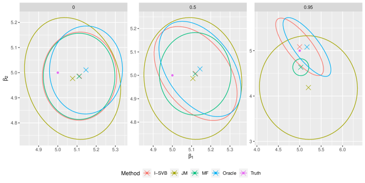
Two-dimensional visualization. To understand the behaviour of the methods, it is helpful to visualise these sets for I-SVB, MF and JM in a $2$-dimensional example. Figure 1 plots a realisation of the credible/confidence regions and estimates from the three methods in three scenarios. We take $n=200$, $p=400$, and define a parameter $\beta^{0}$ with sparsity $s_{0}=10$ and non-zero coordinates given by $\beta_{i}^{0}=5$. We set the first two coordinates of $\beta^{0}$ to be non-zero, and distribute the remaining 8 non-zero coordinates uniformly throughout $\beta^{0}$. The rows of the design are distributed as $X_{i\cdot}\sim^{iid}\mathcal{N}_{p}(0,\Sigma_{\rho}^{AR})$, where the elements of the (autoregressive) covariance matrix are given by $[\Sigma_{\rho}^{AR}]_{ij}=\rho^{|i-j|}$. We vary the correlation between the scenarios, with each facet title giving the value of $\rho$. For comparison, we also plot Oracle confidence sets corresponding to the low-dimensional linear regression model $Y=X_{S_{0}}\beta_{S_{0}}+\varepsilon$, where $S_{0}$ is the (unknown) support of the true $\beta^{0}$. The oracle estimate of the full parameter $\beta$ is given by $\hat{\beta}^{o}_{S_{0}}:=(X_{S_{0}}^{T}X_{S_{0}})^{-1}X_{S_{0}}^{T}Y$ on $S_{0}$, and is a point estimate $\hat{\beta}^{o}_{S_{0}^{C}}=(0,\dots,0)$ outside of $S_{0}$. On $S_{0}$ the oracle covariance matrix is $\Theta_{{S_{0}},{S_{0}}}^{o}=(X_{S_{0}}^{T}X_{S_{0}})^{-1}$, while outside of $S_{0}$ the covariance matrix is 0. The oracle sets are then of the form (24) centered at $\hat{\beta}^{o}_{1:k}$ and with covariance matrix $\Sigma^{o}_{1:k,1:k}$. Note that this is not a valid statistical method since the oracle can not be computed in practice as $S_{0}$ is unknown, but it provides a useful benchmark since one essentially cannot do better than this.

In the first scenario with no correlation (left, $\rho=0$), all the sets have a similar circular shape and contain the truth (pink point). Moreover, MF and I-SVB provide very similar estimates and sets as expected, since there is no underlying correlation. We see there is also little difference between these credible sets and the Oracle confidence region, suggesting they are performing very well in this scenario. JM produces a slightly larger confidence set due to the presence of an inflation factor in the application of their method [25].

However, as we add correlation between the features, the behaviour of the methods diverge. In correlated settings, we see the well-known issue [5, 6] that MF VB both underestimates the marginal variances and fails to capture the correlation, leading to credible sets that are smaller and poorly oriented compared to the Oracle. In the second scenario (middle, $\rho=0.5$) the set still covers the truth, but in the third scenario (right, $\rho=0.95$) it does a poor job of quantifying the uncertainty. In these scenarios, JM increases the size of the confidence sets to account for the added difficulty of the correlation, but it does not seem to pick up the correct covariance structure, leading to much larger confidence regions (though at least covering the truth). In contrast, the I-SVB credible sets seem to capture the correlation structure much more effectively, mirroring the oracle, resulting in sets that are smaller while also covering the truth. Figure 1 demonstrates visually that unlike MF VB, our method I-SVB can correctly pick up (it is close to the oracle) the posterior correlation structure of $\beta_{1:k}$ and provide good estimates of the posterior uncertainty, leading to much improved uncertainty quantification in correlated settings. In Section 6, we provide heuristics to explain why I-SVB appears to perform fairly similarly to the oracle, even in this strongly correlated scenario. Not only is the coverage close to that of the oracle, but the shape of the credible set also nearly matches the oracle shape for AR covariances, as can be predicted from the heuristics.

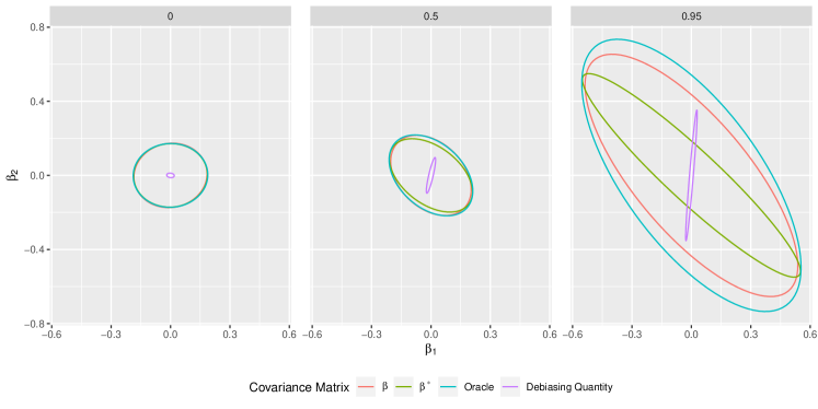
To better understand why I-SVB seems to approach the Oracle covariance, we plot the components of the covariance of $\beta_{1:2}$ under the variational posterior. Recall that in 2 dimensions, the I-SVB posterior is characterised by $\beta_{1:2}=\beta_{1:2}^{*}-(X_{1:2}^{T}X_{1:2})^{-1}X_{1:2}^{T}X_{-2}\beta_{-2}$, where the distributions of $\beta_{1:2}^{*}$ and $\beta_{-2}$ are independent. In Figure 2, we plot the ellipses $\{v\in\mathbb{R}^{2}:v^{T}M^{-1}v=\chi_{0.95,2}\}$ with $M$ given by $(i)$ the I-SVB covariance of $\beta_{1:2}$, $(ii)$ the I-SVB covariance of $\beta_{1:2}^{*}$, $(iii)$ the I-SVB covariance of $(X_{1:2}^{T}X_{1:2})^{-1}X_{1:2}^{T}X_{-2}\beta_{-2}$, and $(iv)$ the Oracle covariance of $\beta_{1:2}$. We see that the covariance contribution from the ‘debiasing’ quantity $(iii)$ alters the covariance of $\beta_{1:2}^{*}$, which is too small, to give a covariance structure for $\beta_{1:2}$ which is closer to the oracle covariance structure. Note this is not a simple inflation factor, since this debiasing occurs by diferent amounts in different directions, and becomes more pronounced as the feature correlation increases. Similar plots with the covariance between features given by the matrix $\Sigma_{\rho}$ are given in Figures 4 and 5 in the supplementary material. Some heuristics about the size of the ‘debiasing’ term can be found in Section 6.

Realisations of 2D credible regions Refer to caption

Figure 1: 95%-credible or confidence regions in three scenarios with design matrix rows $X_{i\cdot}\sim^{iid}\mathcal{N}_{p}(0,\Sigma_{\rho}^{AR})$ for increasing values of $\rho$ given in the title of each facet. The interior of the ellipses represent the credible or confidence regions, the crosses mark their centering and the pink point is the true value of $(\beta_{1},\beta_{2})$. Each scenario has $n=200,p=400,k=2,s_{0}=10$ and $\beta^{0}_{i}=5$.

Covariance structure of the components of $\beta_{1:2}$ Refer to caption

Figure 2: Realisations of the sets $\{v\in\mathbb{R}^{2}:v^{T}M^{-1}v=\chi_{0.95,2}\}$ with $M$ given by the covariance matrices of $\beta_{1:2}$, $\beta_{1:2}^{*}$, the Oracle, and the debiasing quantity ($(X_{1:2}^{T}X_{1:2})^{-1}X_{1:2}^{T}X_{-2}\beta_{-2}$). The design matrix rows are distributed as $X_{i\cdot}\sim^{iid}\mathcal{N}_{p}(0,\Sigma_{\rho}^{AR})$ for increasing values of $\rho$ given in the title of each facet. Each scenario has $n=200,p=400,k=2,s_{0}=10$ and $\beta^{0}_{i}=5$.

Numerical comparison in the multi-dimensional case $k\geq 2$. We now numerically compare these methods in a more systemic fashion, still in the case $\Sigma=\Sigma_{\rho}^{AR}$. We compute the coverage as before, and measure the size of the sets via their $k-$dimensional volume, which is proportional to $\sqrt{\prod_{j=1}^{k}\lambda_{j}}$ where $\{\lambda_{i}\}_{i=1}^{k}$ are the eigenvalues of the covariance matrix defining the regions (e.g. $\hat{\Theta}_{1:k}$ in (24)). To facilitate comparison, when the Oracle gives a non-zero volume we report the relative volume of each method compared to the Oracle (so that in these cases the Oracle has relative volume 1). In some scenarios, where the true parameter of interest contains a 0, the Oracle set is a lower dimensional subspace of $\mathbb{R}^{k}$, and so has volume 0; in these cases we report the relative volume of each method to I-SVB. We also report the average $L_{2}-$error of the estimators (i.e. region centers) over the Monte Carlo simulations.

Each scenario is parametrized by the tuple $(n,p,k,s_{0},\beta^{0}_{j},\rho)$, where all parameters apart from $k$ have the same meaning as before, but we are now interested in $k-$dimensional credible/confidence regions for $\beta_{1:k}$. We also specify the true value of $\beta_{1:k}^{0}$ in each scenario, and distribute the remaining non-zero coordinates uniformly throughout the nuisance parameter $\beta_{-k}^{0}$, where the values of the non-zero coordinates are specified by $\beta_{j}^{0}$. We again simulate 500 realisations of a dataset and compute the credible or confidence sets for each method. Table 2 contains the results.

With no correlation (scenario $(i)$), MF and I-SVB have similar performance to the Oracle — in each case we observe similar coverage, $L_{2}-$error and relative volume close to 1. The JM method likewise achieves good coverage in these scenarios, but with a much larger relative volume to compensate for a larger $L_{2}-$error in the estimate. The JM method also takes much longer to run due to the expensive estimation of $\Sigma^{-1}$.

It is when we add correlation between the features (scenarios $(ii)-(vi)$) that we observe a difference in the behaviour of the non-Oracle methods, similar to what we expect in light of Figure 1. In these scenarios, I-SVB maintains approximately the target coverage, while the coverage achieved by MF and JM drops significantly. Remarkably, we see that the volume of the I-SVB sets is at most 50% larger than the Oracle, and in the higher dimensional scenarios with larger $n$ only about 30% larger. The JM method struggles due to a larger bias in the estimate — it tries to compensate with a much larger relative volume, but this is not enough to increase the coverage. For full MF, the problem is once again that the credible regions are too small, with the relative volume of credible regions plummeting as we increase $k$ and $\rho$, leading to significant underestimates of the uncertainty. We also see that in scenarios $(iv)$ and $(vi)$, where some of the coordinates of $\beta_{1:k}^{0}$ are zero, I-SVB maintains good coverage while providing a volume which is much smaller than JM, suggesting that I-SVB is concentrating on a lower dimensional subspace of $\mathbb{R}^{k}$ as the Oracle does. In summary, I-SVB seems to provide good (scalable) estimation and coverage for $\beta_{1:k}$, while also accurately capturing the underlying correlation, leading to smaller and more informative credible sets.

Scenario $(n,p,k,s_{0},\beta^{0}_{j},\rho)$ Method Cov. $L_{2}-$error Rel. Volume Time
$(i)$ I-SVB 0.960 0.091 ± 0.048 1.007 ± 0.081 0.301 ± 0.107
$(200,400,2,10,\log n,0)$ MF 0.946 0.091 ± 0.048 0.951 ± 0.071 0.162 ± 0.080
$\beta^{0}_{1:2}=(\log n,\log n)$ JM 0.952 0.112 ± 0.065 1.843 ± 0.314 1.012 ± 0.163
Oracle 0.948 0.096 ± 0.065 1.000 ± 0.073 -
$(ii)$ I-SVB 0.966 0.127 ± 0.065 1.517 ± 0.118 0.206 ± 0.040
$(200,400,2,10,\log n,0.5)$ MF 0.790 0.125 ± 0.064 0.532 ± 0.043 0.309 ± 0.071
$\beta^{0}_{1:2}=(\log n,\log n)$ JM 0.742 0.342 ± 0.527 2.975 ± 0.402 6.526 ± 0.902
Oracle 0.950 0.129 ± 0.068 1.000 ± 0.069 -
$(iii)$ I-SVB 0.976 0.130 ± 0.046 1.397 ± 0.122 0.651 ± 0.106
$(400,800,4,10,\log n,0.5)$ MF 0.734 0.129 ± 0.046 0.305 ± 0.029 1.015 ± 1.652
$\beta^{0}_{1:4}=(\log n,\dots,\log n)$ JM 0.430 0.308 ± 0.328 4.194 ± 0.979 32.808 ± 7.427
Oracle 0.972 0.123 ± 0.047 1.000 ± 0.080 -
$(iv)$ I-SVB 0.970 0.110 ± 0.040 1.000 ± 0.091 0.982 ± 0.119
$(400,800,4,10,\log n,0.25)$ MF 0.842 0.342 ± 1.115 0.394 ± 0.028 2.244 ± 0.423
$\beta^{0}_{1:4}=(0,0,\log n,\log n)$ JM 0.500 0.498 ± 0.535 8.727 ± 9.590 31.551 ± 2.089
Oracle 0.990 0.072 ± 0.038 0.000 ± 0.000 -
$(v)$ I-SVB 0.966 0.163 ± 0.052 1.325 ± 0.177 1.591 ± 17.545
$(400,1000,6,12,\log n,0.5)$ MF 0.616 0.246 ± 0.859 0.157 ± 0.016 7.984 ± 63.167
$\beta^{0}_{1:6}=(\log n,\dots,\log n)$ JM 0.144 0.474 ± 0.551 7.304 ± 1.964 32.330 ± 2.805
Oracle 0.936 0.166 ± 0.054 1.000 ± 0.088 -
$(vi)$ I-SVB 0.950 0.366 ± 0.111 1.000 ± 0.157 0.868 ± 0.148
$(400,1000,6,12,\mathcal{U}(-5,5),0.9)$ MF 0.576 0.175 ± 0.136 0.001 ± 0.000 0.531 ± 0.196
$\beta^{0}_{1:6}=(0,\dots,0)$ JM 0.180 0.148 ± 0.090 265.69 ± 5538.8 29.079 ± 11.735
Oracle - - - -
Table 2: Estimation and uncertainty quantification performance for $\beta_{1:k}$ using 3 methods and the Oracle approach. Highlighted in bold are the smallest relative volume (compared to the Oracle) of the sets, subject to coverage being larger than 0.85, and the smallest mean $L_{2}$-error. We do not highlight the Oracle since it is not a valid method as it depends on the unknown truth, while in (iv) it reduces to the point estimate at 0, hence we omit it.

4.3 Real covariate example: riboflavin dataset

We conclude by using real covariates from the riboflavin dataset [8] with simulated responses. The dimension of the covariate data $X$ is $n=71$ and $p=4088$, and the pairwise correlation between features ranges from close to -1 to close to +1. We sample 500 realisations of the dataset $Y=X\beta^{0}+\epsilon$ (holding $X$ and $\beta^{0}$ fixed) computing the corresponding $95\%$-credible/confidence regions for each method. We take $k=1$ and consider as target parameter $\beta_{j}$, i.e. we do not necessarily take $j=1$. Since the design is fixed, the different covariate columns of $X$ have very different structures and hence the performance of each method depends on this choice. To provide a fair comparison, we sample a random subset of the coordinates of size 100, compute estimates of the coverage for each method on each coordinate using 500 realisations of the data, and report the mean performance over the 100 coordinates. Results are given in Table 3, with the Oracle included for reference.

In the first example, we set both $\beta_{j}^{0}=\log n$ and the other active coordinates $\beta_{k}^{0}=\log n$. In this case, we see that I-SVB and ZZ both offer good coverage, with the I-SVB coverage slightly below the intended level. Of the non-oracle methods, I-SVB offers the smallest MAE, and the credible intervals produced by this method are nearly the same size as the Oracle intervals, showing good uncertainty quantification. The mean-field method struggles in this scenario, as the complex correlation structure between features throws off the modelling of the nuisance parameter and the credible intervals are too small. The ZZ method offers high coverage, but the confidence sets produced by this method are very wide, and the estimate itself is more biased than for I-SVB. The JM method struggles due to a large bias and the confidence intervals have low coverage despite being quite large.

In the second example, we set the coordinate of interest $\beta_{j}^{0}=0$, with the other active coordinates given by $\beta_{k}^{0}=\log n$. In this case, the I-SVB coverage drops, though not too dramatically. The MF method performs very well in this scenario, which is understandable since the prior contains a spike at 0 and it can often detect that the truth is zero; the MAE is very small and the credible intervals are the smallest of the non-oracle methods. The ZZ method once again yields very high coverage, but it is again conservative due to the very long intervals. Likewise, the JM method offers high coverage, but with rather long credible intervals.

Scenario $(n,p,s_{0},\beta_{j}^{0},\beta_{k}^{0})$ Method Cov. MAE Length Time
riboflavin $(i)$ I-SVB 0.905 0.159 ± 0.127 0.614 ± 0.021 2.129 ± 0.275
$(71,4088,5,\log n,\log n)$ MF 0.262 2.078 ± 0.931 0.463 ± 0.002 1.828 ± 0.422
ZZ 0.971 0.422 ± 0.250 4.691 ± 1.465 0.656 ± 0.162
JM 0.300 2.430 ± 0.135 1.907 ± 0.103 22.573 ± 3.304
Oracle 0.944 0.125 ± 0.093 0.613 ± 0.000 -
riboflavin $(ii)$ I-SVB 0.857 0.196 ± 0.154 0.646 ± 0.022 3.209 ± 0.511
$(71,4088,5,0,\log n)$ MF 0.976 0.042 ± 0.032 0.450 ± 0.005 4.884 ± 7.862
ZZ 1.000 0.174 ± 0.131 4.664 ± 1.380 2.650 ± 4.094
JM 0.992 0.078 ± 0.033 1.408 ± 0.15 14.177 ± 2.483
Oracle 1.000 0.000 ± 0.000 0.000 ± 0.000 -
Table 3: Estimates of the coverage, MAE and length of the credible intervals produced using simulated data with the covariates from the riboflavin dataset. Highlighted in bold are the smallest interval length, subject to coverage being larger than 0.85, and the smallest MAE.

5 Discussion

In summary, we propose here a scalable variational Bayes approach for inference of a low-dimensional parameter in sparse high-dimensional linear regression. Our approach combines a simple preprocessing step with a variational class tailored to this problem, allowing one to plug-in existing computational tools for fast and simple computation. We demonstrate that our I-SVB method significantly improves on standard mean-field variational inference for this task, and performs favourably compared to two frequentist counterparts in terms of both estimation accuracy and uncertainty quantification. The I-SVB method demonstrates robustness to correlated features, various forms of signal, and even extends naturally to multidimensional uncertainty quantification. In general, I-SVB produces estimates which are less biased than the frequentist estimators and credible regions which are suitably more confident — though crucially not overconfident (i.e. wrong) like the standard mean-field approach. Furthermore, I-SVB produces multidimensional credible regions which are very close to optimal ‘oracle’-type confidence sets across a variety of scenarios. Our empirical results are supported by theoretical frequentist guarantees in the form of a Bernstein-von Mises theorem.

Acknowledgements. We wish to thank the Imperial College London-CNRS PhD Joint Programme for funding to support this collaboration, including funding ALH’s PhD position. IC’s work is partly supported by ANR grant project ANR-23-CE40-0018-01 (BACKUP) and an Institut Universitaire de France fellowship.

6 Heuristics

We provide some heuristic computations to explain the excellent behaviour of the I-SVB method in the simulations above in settings with possibly significant correlation. Making these heuristics rigorous is an interesting topic for future work. As above, suppose $X_{i\cdot}\sim\mathcal{N}(0,\Sigma)$ with $\Sigma=\Sigma^{AR}_{\rho}$ or $\Sigma=\Sigma_{\rho}$ for a fixed $\rho\in[0,1)$. Recall that the cases where either $\rho=0$ or $\rho=\rho_{n}=o(1)$ vanishes sufficiently fast are covered by our theoretical results from Section 3.

Let us focus on the one-dimensional case and compare the variance of the oracle ‘estimator’ $\hat{\beta}^{o}_{S_{0}}:=(X_{S_{0}}^{T}X_{S_{0}})^{-1}X_{S_{0}}^{T}Y$ with the expected variance of the I-SVB variational distribution. We assume for simplicity that the coordinate of interest $\beta_{1}$ belongs to $S_{0}$. We have

$$\text{Var}(\hat{\beta}^{o}_{S_{0}}|X)=(X_{S_{0}}^{T}X_{S_{0}})^{-1}\sim(\Sigma_{S_{0}})^{-1}/n,$$

where $\Sigma_{S_{0}}$ is the submatrix of $\Sigma$ obtained by restricting (both) indices to $S_{0}$. If $v^{o}_{1}$ denotes the (unconditional) variance of the oracle estimate on the first coordinate, we also have

$$v^{o}_{1}\sim[(\Sigma_{S_{0}})^{-1}]_{11}/n.$$ (25)

Recall on the other hand that I-SVB models $\beta_{1}^{*}$ and $\beta_{-1}$ independently by $\beta_{1}^{*}\sim\mathcal{N}(X_{1}^{T}Y/\|X_{1}\|_{2}^{2},\|X_{1}\|_{2}^{-2})$ and with $\beta_{-1}$ following a mean-field approximation of the posterior of $\beta_{-1}|Y$. Since we use the model $\check{Y}=\check{W}\beta_{-1}+\check{\varepsilon}$ to fit the variational posterior on $\beta_{-1}$, in these heuristics we assume that the posterior correctly recovers the true support $S_{0}^{-}:=S_{0}\backslash\{1\}$ of $\beta_{-1}^{0}$ and that, on $S_{0}^{-}$, it mimics the behaviour of the oracle estimate $\hat{\beta}^{o}_{S_{0}^{-}}=(\check{W}^{T}_{S_{0}^{-}}\check{W}_{S_{0}^{-}})^{-1}\check{W}_{S_{0}^{-}}\check{Y}$ in the projected model. In practice, there may be some uncertainty in terms of the support, which will then generate extra variance for I-SVB. As before, $\hat{\beta}^{o}_{S_{0}^{-}}\approx\mathcal{N}(\beta^{0}_{S_{0}^{-}},(\check{W}_{S_{0}^{-}}^{T}\check{W}_{S_{0}^{-}})^{-1})$, and the mean-field VB posterior should be close to the best mean-field normal approximation of this Gaussian distribution, which is the normal distribution with diagonal precision matrix matching the diagonal of the matrix $\check{W}_{S_{0}^{-}}^{T}\check{W}_{S_{0}^{-}}$, that is the precision corresponding to the oracle variance $(\check{W}_{S_{0}^{-}}^{T}\check{W}_{S_{0}^{-}})^{-1}$ of $\hat{\beta}^{o}_{S_{0}^{-}}$ (see e.g. [44], Lemma 8). One thus expects the covariance of the mean-field VB distribution $\hat{Q}_{-1}$ on $\beta_{-1}$ to be close to the diagonal matrix $\text{Diag}(1/[\check{W}_{S_{0}^{-}}^{T}\check{W}_{S_{0}^{-}}]_{ii}])$, where we have $\check{W}_{S_{0}^{-}}^{T}\check{W}_{S_{0}^{-}}=X_{S_{0}^{-}}^{T}(I_{n}-H)X_{S_{0}^{-}}\approx n\Sigma_{S_{0}^{-}}-\|X_{1}\|_{2}^{2}\gamma_{-1}\gamma_{-1}^{T}$, so that $\text{Diag}(1/[\check{W}_{S_{0}^{-}}^{T}\check{W}_{S_{0}^{-}}]_{ii}])\approx\frac{1}{n}\cdot\textrm{Diag}(1/([\Sigma_{S_{0}^{-}}]_{ii}-\gamma_{i}^{2}))$. Since $\beta_{1}=\beta_{1}^{*}-\sum_{i=2}^{p}\gamma_{i}\beta_{i}$ by definition, the overall expected variance of I-SVB on $\beta_{1}$ is, with $\gamma_{-1}^{T}:=(\gamma_{i})_{i\in S_{0}^{-}}$,

$\displaystyle v^{\operatorname{\it{I-SVB}}}_{1}\approx\frac{1}{\|X_{1}\|_{2}^{2}}+\text{Var}_{\hat{Q}_{1}}\Big{(}\sum_{i\in S_{0}^{-}}\gamma_{i}\beta_{i}\Big{)}$ $\displaystyle=\frac{1}{\|X_{1}\|_{2}^{2}}+\gamma_{-1}^{T}\text{Var}_{\hat{Q}_{1}}(\beta_{-1})\gamma_{-1}$
$\displaystyle\approx\frac{1}{n}\left\{1/\Sigma_{11}+\sum_{i\in S_{0}^{-}}\gamma_{i}^{2}/([\Sigma_{S_{0}^{-}}]_{ii}-\gamma_{i}^{2})\right\},$ (26)

where we have used the mean-field approximation by taking the above diagonal variance for $\beta_{-1}$ under $\hat{Q}_{1}$.

By the same reasoning based on the (diagonal) precision of the MF VB–approximation matching the diagonal precision of the oracle, the first term $1/(n\Sigma_{11})$ in (26) corresponds to the expected variance of the full MF VB approximation based on the spike-and-slab prior (again assuming the posterior recovers the true support). In particular, while the MF variational posterior has an asymptotic variance which is too small in correlated settings, and therefore corresponding credible intervals typically undercover, we see in (26) that since the terms of the sum are positive, the variance of I-SVB is always larger, and hence this results in I-SVB credible intervals having typically better coverage than their MF counterparts. We now further investigate quantitatively how much variance is gained in (26) for I-SVB for $\Sigma=\Sigma^{AR}_{\rho}$ and $\Sigma=\Sigma_{\rho}$.

Case $\Sigma=\Sigma^{AR}_{\rho}$. Suppose as assumed in the simulations above that we are in a ‘least-favourable’ situation that maximises correlation between features within $S_{0}$, which corresponds to $S_{0}=\{1,2,\ldots,s_{0}\}$ (in case $S_{0}$ does not have coordinates amongs the first integers, for instance if $S_{0}$ is drawn uniformly at random in $\{1,\ldots,p\}$, the corresponding covariance of $(X_{i})_{i\in S_{0}}$ will typically be close to the identity as $\rho^{q}$ is small for large $q$, and so this is closer in spirit to the setting with low correlation already studied in Section 3). The matrix $\Sigma=\Sigma^{AR}_{\rho}$ can easily be seen to have a tridiagonal inverse and $v^{o}_{1}=[\Sigma_{S_{0}}^{-1}]_{11}/n=n^{-1}/(1-\rho^{2})$. On the other hand, by the law of large numbers $\gamma_{j}\approx E(X_{11}X_{1j})=\rho^{j-1}$, so for $s_{0}\geq 2$

$$v^{\operatorname{\it{I-SVB}}}_{1}\approx\frac{1}{n}\left\{\frac{1}{\Sigma_{11}}+\sum_{i\in S_{0}^{-}}\frac{\gamma_{i}^{2}}{([\Sigma_{S_{0}^{-}}]_{ii}-\gamma_{i}^{2})}\right\}=\frac{1}{n}\left\{\frac{1}{1-\rho^{2}}+\sum_{j=2}^{s_{0}-1}\frac{\rho^{2j}}{1-\rho^{2j}}\right\},$$

where the first term in brackets corresponds to the oracle variance, and the second part of the sum is always greater than 0 and small unless $\rho$ is very close to $1$. If $s_{0}=2$ (and the sum is empty) we even have $v^{\operatorname{\it{I-SVB}}}_{1}\approx v_{1}^{o}$. The last display shows that the variance of I-SVB nearly matches that of the oracle, as seen empirically in the simulations above, while the MF method has $v^{MF}_{1}\approx 1/n$ leading to undercoverage. The same heuristics also apply in two dimensions ($k=2$). In that case, it can be checked by a similar reasoning as above that, denoting by $v_{1:2}^{o}$ and $v_{1:2}^{\operatorname{\it{I-SVB}}}$ respectively the variance of the oracle and the expected variance of I-SVB, one has, with $c_{\rho}=1/(1-\rho^{2})$,

$$v_{1:2}^{o}=(c_{\rho}/n)\begin{bmatrix}1&-\rho\\ -\rho&1+\rho^{2}\end{bmatrix},\qquad v_{1:2}^{\operatorname{\it{I-SVB}}}\approx v_{1:2}^{0}+(c_{\rho}/n)\left[\begin{matrix}0&0\\ 0&\sum_{j=2}^{s_{0}-1}\frac{\rho^{2j}}{1-\rho^{2j}}\end{matrix}\right],$$

so that once again the variance of I-SVB equals the oracle variance plus a term which will be small for moderate values of $\rho$. These findings are in line with the empirical observations in Section 4.2 above: I-SVB credible ellipses nearly match the oracle confidence ellipses associated to the oracle estimator, as seen in Figure 1. Also, in this setting, the standard MF approximation, which has a diagonal variance, is necessarily far off the oracle variance as in the above display. We note also that the asymptotic variance of $\beta_{1:2}^{*}$ is

$$\text{Var}(\beta_{1:2}^{*})=(c_{\rho}/n)\begin{bmatrix}1&-\rho\\ -\rho&1\end{bmatrix},$$

which is different from $v_{1:2}^{o}\approx v_{1:2}^{\operatorname{\it{I-SVB}}}$. This confirms that in this case ‘undoing the transformation’ from $\beta_{1:2}^{*}$ to $\beta_{1:2}$ has a non-negligible effect in terms of variance, as can be seen empirically in Figure 2.

Case $\Sigma=\Sigma_{\rho}$. By arguing similarly as in the AR case, one first computes explicitly the precision matrix $(\Sigma_{S_{0}})^{-1}$ which again is available in explicit form and which leads (we omit the details) to $n\cdot v_{1}^{o}\sim[(\Sigma_{S_{0}})^{-1}]_{11}=e_{\rho}/(1-\rho)$, with $e_{\rho}=(1-2\rho+\rho s_{0})/(1-\rho+\rho s_{0})$ and $e_{\rho}\approx 1$ for ‘large’ $s_{0}$. On the other hand, $v_{1}^{MF}\approx(\Sigma_{11})^{-1}/n=1/n$ and $v_{1}^{\operatorname{\it{I-SVB}}}\approx(1+(s_{0}-1)\rho^{2}/(1-\rho^{2}))/n$. In this setting with strong correlations, we still have that $v_{1}^{\operatorname{\it{I-SVB}}}$ is typically significantly larger than $v_{1}^{MF}$, thus compensating for the undercoverage of classical mean-field VB. This time, the expected variance of I-SVB does not match in general that of the oracle. One can note though that $v_{1}^{\operatorname{\it{I-SVB}}}$ scales (if $\rho$ is bounded away from 00 so that $\rho^{2}/(1+\rho)>0$ is a constant) as $s_{0}(1-\rho)^{-1}/n$, which is $s_{0}$ times the oracle variance, so in an (idealised) $s_{0}\to\infty$ limit (and assuming the centering of I-SVB is roughly of correct order) we have over-coverage; this is less critical compared to the under-coverage of MF-VB, as then the method is simply somewhat conservative (so credible sets may be slightly too large) but is then expected at least to cover the true parameter, which once again is in line with the empirical results observed in Table 1.

7 Proofs

In this section we prove the theoretical results presented in the main text.

7.1 Proofs for the one dimensional case $k=1$

Proof of Lemma 1.

Recall that we have the following decomposition for the likelihood

$\displaystyle\mathcal{L}_{n}(\beta,Y)\propto e^{-\frac{1}{2}\|X_{1}\|^{2}_{2}(\beta_{1}^{*}-\frac{X_{1}^{T}Y}{\|X_{1}\|_{2}^{2}})^{2}}e^{-\frac{1}{2}\|\check{W}\beta_{-1}-\check{Y}\|_{2}^{2}},$

where $\check{W},\check{Y}$ are defined in (6). Using this decomposition and the form of the prior (5), we deduce that for any $f_{1}:\mathbb{R}\rightarrow\mathbb{R}^{+}$ and $f_{2}:\mathbb{R}^{p-1}\rightarrow\mathbb{R}^{+}$ measurable, we have

$\displaystyle E(f_{1}(\beta_{1}^{*})f_{2}(\beta_{-1})|Y)$ $\displaystyle\propto\int_{\mathbb{R}^{p}}f_{1}(\beta_{1}^{*})f_{2}(\beta_{-1})e^{-\frac{1}{2}\|X_{1}\|^{2}_{2}(\beta_{1}^{*}-\frac{X_{1}^{T}Y}{\|X_{1}\|_{2}^{2}})^{2}}e^{-\frac{1}{2}\|\check{W}\beta_{-1}-\check{Y}\|_{2}^{2}}g(\beta_{1}^{*})d\beta_{1}dMS_{p-1}(\nu,\lambda)(\beta_{-1})$
$\displaystyle\propto\int_{\mathbb{R}}f_{1}(u)e^{-\frac{1}{2}\|X_{1}\|^{2}_{2}(u-\frac{X_{1}^{T}Y}{\|X_{1}\|_{2}^{2}})^{2}}g(u)du\int_{\mathbb{R}^{p-1}}f_{2}(\beta_{-1})e^{-\frac{1}{2}\|\check{W}\beta_{-1}-\check{Y}\|_{2}^{2}}dMS_{p-1}(\nu,\lambda)(\beta_{-1}).$

This implies that, under the posterior distribution, $\beta_{-1}$ and $\beta_{1}^{*}$ are independent and their distributions are given by (7) and (8) respectively. The assertion regarding the specific Examples 2 and 3 can be easily deduced from (8) when $g$ has the specific form chosen in Examples 2 and 3.

For the frequentist distribution of $\check{Y}$ under $P_{0}$, note that $\check{Y}=P^{T}Y=P^{T}(X\beta^{0}+\varepsilon)=P^{T}(X_{-1}\beta^{0}_{-1}+\varepsilon)=\check{W}\beta^{0}_{-1}+P^{T}\varepsilon$ and thus $\check{Y}\sim\mathcal{N}(\check{W}\beta^{0}_{-1},P^{T}P)=\mathcal{N}(\check{W}\beta^{0}_{-1},I_{n-1})$. ∎

Proof of Theorem 1.

Step 1: Convergence of $\beta_{-1}$ to $\beta^{0}_{-1}$. Recall that the VB posterior $\hat{Q}_{-1}$ for $\beta_{-1}$ is the mean-field approximation of $\beta_{-1}$ based on the variational family $\mathcal{Q}_{-1}$ in (9). By Lemma 1, the posterior for $\beta_{-1}$ equals the posterior distribution in the linear regression model $\check{Y}=\check{W}\beta_{-1}+\check{\varepsilon}$ with model selection prior $MS_{p-1}(\nu,\lambda)$. Thus we are exactly in the setting studied in Ray and Szabó [35], applied to this transformed linear regression model. Since $\beta^{0}$ satisfies the compatibility conditions (18) and the prior satisfies (4), (17) and $\lambda=O(\|\check{W}\|\sqrt{\log(p-1)}/s_{0})$, applying Theorem 1 in [35] gives that there exists $M>0$ large enough depending only on the prior such that, with $\varepsilon_{n}=M\frac{\rho_{n}s_{0}\sqrt{\log p}}{\|\check{W}\|c_{0}^{3}}$,

$\displaystyle\hat{Q}_{-1}\left(\{\beta_{-1}\in\mathbb{R}^{p-1},||\beta_{-1}-\beta_{-1}^{0}||_{1}\leq\varepsilon_{n}\}\right)=1+o_{P}(1).$ (27)

Using that $\|\check{W}\|=\|(I-H)X_{-1}\|$ and (19), the rate $\varepsilon_{n}$ satisfies

$\displaystyle\varepsilon_{n}\|X_{1}\|_{2}\max_{i=2,\dots,p}|\gamma_{i}|\rightarrow 0.$ (28)

Step 2: Showing asymptotic normality. Denote $B_{n}=\{\beta_{-1}\in\mathbb{R}^{p-1}:\|\beta_{-1}-\beta^{0}_{-1}\|_{1}\leq\varepsilon_{n}\}$, $A_{n}=\mathbb{R}\times B_{n}$ and let $E^{\hat{Q}}$ be the expectation under the variational posterior $\hat{Q}$. By Lemma 1 and (27), we have $\hat{Q}(A_{n})=\hat{Q}_{-1}(B_{n})=1+o_{P}(1)$. To prove a convergence result as in (16), we employ the technique consisting in showing that for all $t\in\mathbb{R}$, the VB posterior Laplace transform $I_{n}:=E^{\hat{Q}}(e^{t\|X_{1}\|_{2}(\beta_{1}-\hat{\beta}_{1})}1_{A_{n}})$, restricted to the set $A_{n}$ on which $\hat{Q}$ concentrates with $P_{0}$-probability one, converges to that of the limiting Gaussian, which then implies the result (see [37] and [11]). First,

$\displaystyle I_{n}$ $\displaystyle=E^{\hat{Q}}(e^{t\|X_{1}\|_{2}(\beta_{1}^{*}-\hat{\beta}_{1}-\sum_{i=2}^{p}\gamma_{i}\beta_{i})}1_{A_{n}})=E^{\hat{Q}}(e^{t\|X_{1}\|_{2}(\beta_{1}^{*}-\hat{\beta}_{1}-\sum_{i=2}^{p}\gamma_{i}\beta_{i}^{0}-\sum_{i=2}^{p}\gamma_{i}(\beta_{i}-\beta_{i}^{0}))}1_{A_{n}}).$

Since $\hat{\beta}_{1}+\sum_{i=2}^{p}\gamma_{i}\beta_{i}^{0}=\frac{X_{1}^{T}Y}{\|X_{1}\|_{2}^{2}}$ and using that $\beta_{1}^{*}$ and $\beta_{-1}$ are independent under $\hat{Q}$, we deduce that

$\displaystyle I_{n}$ $\displaystyle=E^{\hat{Q}}(e^{t\|X_{1}\|_{2}(\beta_{1}^{*}-\frac{X_{1}^{T}Y}{\|X_{1}\|_{2}^{2}}-\sum_{i=2}^{p}\gamma_{i}(\beta_{i}-\beta_{i}^{0}))}1_{\{\beta_{-1}\in B_{n}\}})$
$\displaystyle=E^{\hat{Q}}(e^{t\|X_{1}\|_{2}(\beta_{1}^{*}-\frac{X_{1}^{T}Y}{\|X_{1}\|_{2}^{2}})})E^{\hat{Q}}(e^{-t\|X_{1}\|_{2}\sum_{i=2}^{p}\gamma_{i}(\beta_{i}-\beta_{i}^{0}))}1_{\{\beta_{-1}\in B_{n}\}}).$ (29)

For the first term, recall that $\beta_{1}^{*}\sim\pi(\beta_{1}^{*}|Y)$ has the same distribution as the posterior under $\hat{Q}$ by (11). Thus by Lemma 1 and making the change of variable $u\rightarrow\frac{u}{\|X_{1}\|_{2}}+\frac{X_{1}^{T}Y}{\|X_{1}\|_{2}^{2}}$, we have

$\displaystyle E^{\hat{Q}}\left[e^{t\|X_{1}\|_{2}(\beta_{1}^{*}-\frac{X_{1}^{T}Y}{\|X_{1}\|_{2}^{2}})}\right]$ $\displaystyle=\frac{\int_{\mathbb{R}}e^{t\|X_{1}\|_{2}\left(u-\frac{X_{1}^{T}Y}{\|X_{1}\|_{2}^{2}}\right)}e^{-\frac{\|X_{1}\|_{2}^{2}}{2}\left(u-\frac{X_{1}^{T}Y}{\|X_{1}\|_{2}^{2}}\right)^{2}}g(u)du}{\int_{\mathbb{R}}e^{-\frac{\|X_{1}\|_{2}^{2}}{2}\left(u-\frac{X_{1}^{T}Y}{\|X_{1}\|_{2}^{2}}\right)^{2}}g(u)du}$
$\displaystyle=\frac{\int_{\mathbb{R}}e^{tu}e^{-\frac{u^{2}}{2}}g\left(\frac{u}{\|X_{1}\|_{2}}+\frac{X_{1}^{T}Y}{\|X_{1}\|_{2}^{2}}\right)du}{\int_{\mathbb{R}}e^{-\frac{u^{2}}{2}}g\left(\frac{u}{\|X_{1}\|_{2}}+\frac{X_{1}^{T}Y}{\|X_{1}\|_{2}^{2}}\right)du}.$

Now using the fact that

$\displaystyle g\left(\frac{u}{\|X_{1}\|_{2}}+\frac{X_{1}^{T}Y}{\|X_{1}\|_{2}^{2}}\right)=g\left(\frac{X_{1}^{T}Y}{\|X_{1}\|_{2}^{2}}\right)e^{\log g\left(\frac{u}{\|X_{1}\|_{2}}+\frac{X_{1}^{T}Y}{\|X_{1}\|_{2}^{2}}\right)-\log g\left(\frac{X_{1}^{T}Y}{\|X_{1}\|_{2}^{2}}\right)},$

that $\log g$ is $c$-Lipschitz with $c=o(\|X_{1}\|_{2})$ and the dominated convergence theorem, we have

$\displaystyle E^{\hat{Q}}\left[e^{t\|X_{1}\|_{2}\left(\beta_{1}^{*}-\frac{X_{1}^{T}Y}{\|X_{1}\|_{2}^{2}}\right)}\right]\leq\frac{\int_{\mathbb{R}}e^{tu}e^{-\frac{1}{2}u^{2}}e^{c\frac{|u|}{\|X_{1}\|_{2}}}du}{\int_{\mathbb{R}}e^{-\frac{1}{2}u^{2}}e^{-c\frac{|u|}{\|X_{1}\|_{2}}}du}=e^{\frac{t^{2}}{2}}(1+o(1))$ (30)

as $\|X_{1}\|_{2}\to\infty$. Combining (30) with (7.1) yields

$\displaystyle I_{n}$ $\displaystyle\leq e^{\frac{t^{2}}{2}}E^{\hat{Q}}(e^{|t|\|X_{1}\|_{2}\max_{i=2,\dots,p}|\gamma_{i}|\|\beta_{-1}-\beta_{-1}^{0}\|_{1}}1_{\{\beta_{-1}\in B_{n}\}})(1+o(1))$
$\displaystyle\leq e^{\frac{t^{2}}{2}}e^{|t|\|X_{1}\|_{2}\max_{i=2,\dots,p}|\gamma_{i}|\varepsilon_{n}}\hat{Q}(A_{n})(1+o(1))=e^{\frac{t^{2}}{2}}(1+o_{P}(1))$

where we used (28) in the last equality. The lower bound $I_{n}\geq e^{\frac{t^{2}}{2}}(1+o_{P}(1))$ follows similarly. Thus we deduce that $I_{n}=e^{\frac{t^{2}}{2}}(1+o_{P}(1))$. Since convergence of the Laplace transform $I_{n}$ for all $t\in\mathbb{R}$ implies weak convergence (cf [37] or [11]), this yields the result. ∎

Proof of Lemma 2.

The Gaussian prior $g\sim\mathcal{N}(0,\sigma_{n}^{2})$ we consider here satisfies all the conditions of Theorem 1, except that $\log g$ is not Lipschitz. Thus to prove Lemma 2, we need just make some small adjustments to the proof of Theorem 1. Step 1 holds as before, while Step 2 holds until (7.1). The only difference is then the calculations for the first term in (7.1). Since $\beta_{1}^{*}|Y\sim\mathcal{N}\left(\frac{\sigma_{n}^{2}X_{1}^{T}Y}{\|X_{1}\|_{2}^{2}\sigma_{n}^{2}+1},\frac{\sigma_{n}^{2}}{\|X_{1}\|_{2}^{2}\sigma_{n}^{2}+1}\right)$ under the posterior, and hence also under $\hat{Q}$ by (11), and $X_{1}^{T}Y=X_{1}^{T}X\beta^{0}+X_{1}^{T}\varepsilon=\|X_{1}\|_{2}^{2}\beta_{1}^{0}+\|X_{1}\|_{2}^{2}\sum_{i=2}^{p}\gamma_{i}\beta_{i}^{0}+X_{1}^{T}\varepsilon$ under $P_{0}$,

$\displaystyle E^{\hat{Q}}\left[e^{t\|X_{1}\|_{2}(\beta_{1}^{*}-\frac{X_{1}^{T}Y}{\|X_{1}\|_{2}^{2}})}\right]$ $\displaystyle=\exp\left(t\|X_{1}\|_{2}\left[\frac{\sigma_{n}^{2}X_{1}^{T}Y}{\|X_{1}\|_{2}^{2}\sigma_{n}^{2}+1}-\frac{X_{1}^{T}Y}{\|X_{1}\|_{2}^{2}}\right]+\frac{t^{2}}{2}\frac{\|X_{1}\|_{2}^{2}\sigma_{n}^{2}}{\|X_{1}\|_{2}^{2}\sigma_{n}^{2}+1}\right)$
$\displaystyle=\exp\left(-t\frac{X_{1}^{T}Y}{(\|X_{1}\|_{2}^{2}\sigma_{n}^{2}+1)\|X_{1}\|_{2}}+\frac{t^{2}}{2}\frac{\|X_{1}\|_{2}^{2}\sigma_{n}^{2}}{\|X_{1}\|_{2}^{2}\sigma_{n}^{2}+1}\right)$
$\displaystyle=\exp\left(-t\|X_{1}\|_{2}\frac{\beta_{1}^{0}+\sum_{i=2}^{p}\gamma_{i}\beta_{i}^{0}}{\|X_{1}\|_{2}^{2}\sigma_{n}^{2}+1}-t\frac{X_{1}^{T}\varepsilon}{(\|X_{1}\|_{2}^{2}\sigma_{n}^{2}+1)\|X_{1}\|_{2}}+\frac{t^{2}}{2}\frac{\|X_{1}\|_{2}^{2}\sigma_{n}^{2}}{\|X_{1}\|_{2}^{2}\sigma_{n}^{2}+1}.\right).$

Using the assumptions (20) and the fact that $\frac{X_{1}^{T}\varepsilon}{(\|X_{1}\|_{2}^{2}\sigma_{n}^{2}+1)\|X_{1}\|_{2}}\sim\mathcal{N}(0,(\|X_{1}\|_{2}^{2}\sigma_{n}^{2}+1)^{-2})=o_{P}(1)$, one deduces that $E^{\hat{Q}}(e^{t\|X_{1}\|_{2}(\beta_{1}^{*}-\frac{X_{1}^{T}Y}{\|X_{1}\|_{2}^{2}})})=e^{\frac{t^{2}}{2}}(1+o_{P}(1))$. Following the rest of the proof of Theorem 1 yields the result. ∎

7.2 Proofs for the k-dimensional cases

To prove Theorem 3, we first need the following Lemma, which is a $k-$dimensional version of Lemma 1.

Lemma 3 (Posterior distribution for $k\geq 1$).

Let $\Pi$ be the prior (12). Then under the posterior distribution, $\beta_{-k}$ and $\beta_{1:k}^{*}$ are independent, and their distributions takes the form

$\displaystyle d\pi(\beta_{-k}|Y)$ $\displaystyle\propto{e^{-\frac{1}{2}\|\check{W}_{k}\beta_{-k}-\check{Y}_{k}\|^{2}_{2}}}dMS_{p-k}(\nu,\lambda)(\beta_{-k}),$ (31)
$\displaystyle d\pi(\beta_{1:k}^{*}|Y)$ $\displaystyle\propto e^{-\frac{1}{2}(\beta_{1:k}^{*}-\Sigma_{k}X_{1:k}^{T}Y)^{T}\Sigma_{k}^{-1}(\beta_{1:k}^{*}-\Sigma_{k}X_{1:k}^{T}Y)}g(\beta_{1:k}^{*})d\beta_{1:k}^{*}.$ (32)

Under the frequentist assumption $Y\sim\mathcal{N}_{n}(X\beta^{0},I_{n})$, we have $\check{Y}_{k}\sim\mathcal{N}(\check{W}_{k}\beta^{0}_{-k},I_{n-k})$.

Proof of Lemma 3.

Recall that we have the following decomposition for the likelihood

$\displaystyle\mathcal{L}_{n}(\beta,Y)\propto\exp\left\{-\frac{1}{2}\left\|H_{k}Y-X_{1:k}\beta_{1:k}^{*}\right\|_{2}^{2}\right\}\cdot\exp\left\{-\frac{1}{2}\|\check{Y}_{k}-\check{W}_{k}\beta_{-k}\|_{2}^{2}\right\}.$

Using this decomposition and the form of the prior, we deduce that for any $f_{1}:\mathbb{R}^{k}\rightarrow\mathbb{R}^{+}$ and $f_{2}:\mathbb{R}^{p-k}\rightarrow\mathbb{R}^{+}$ mesurable, we have

$\displaystyle E(f_{1}(\beta_{1:k}^{*})f_{2}(\beta_{-k})|Y)$ $\displaystyle\propto\int_{\mathbb{R}^{p}}f_{1}(\beta_{1:k}^{*})f_{2}(\beta_{-k})e^{-\frac{1}{2}\left\|H_{k}Y-X_{1:k}\beta_{1:k}^{*}\right\|_{2}^{2}}e^{-\frac{1}{2}\|\check{Y}_{k}-\check{W}_{k}\beta_{-k}\|_{2}^{2}}g(\beta_{1:k}^{*})d\beta_{1:k}^{*}dMS_{p-k}(\nu,\lambda)(\beta_{-k})$
$\displaystyle\propto\int_{\mathbb{R}^{k}}f_{1}(\beta_{1:k}^{*})e^{-\frac{1}{2}\left\|H_{k}Y-X_{1:k}\beta_{1:k}^{*}\right\|_{2}^{2}}g(\beta_{1:k}^{*})d\beta_{1:k}^{*}$
$\displaystyle\quad\times\int_{\mathbb{R}^{p-k}}f_{2}(\beta_{-k})e^{-\frac{1}{2}\|\check{Y}_{k}-\check{W}_{k}\beta_{-k}\|_{2}^{2}}dMS_{p-k}(\nu,\lambda)(\beta_{-k}).$

This implies that, under the posterior distribution, $\beta_{-k}$ and $\beta_{1:k}^{*}$ are independent and their distributions are given by (31) and (32), respectively.

For the frequentist distribution of $\check{Y}$ under $P_{0}$, note that $\check{Y}_{k}=P^{T}_{k}Y=P^{T}_{k}(X_{-k}\beta^{0}_{-k}+\varepsilon)=\check{W}_{k}\beta^{0}_{-k}+P^{T}_{k}\varepsilon$ and thus $\check{Y}_{k}\sim\mathcal{N}(\check{W}_{k}\beta^{0}_{-k},P^{T}_{k}P_{k})=\mathcal{N}(\check{W}_{k}\beta^{0}_{-k},I_{n-k})$ under the frequentist assumption. ∎

Proof of Theorem 3.

The proof is very similar to the proof of Theorem 1.

Step 1: Convergence of $\beta_{-k}$ to $\beta^{0}_{-k}$. Recall that the variational posterior of $\beta_{-k}$, $\hat{Q}_{-k}$, is the mean-field approximation of the posterior distribution of $\beta_{-k}$ which is distributed according to the posterior distribution in a linear regression model induced by the model selection prior $MS_{p-k}(\nu,\lambda)$. Since $\beta^{0}$ satisfies (22), the prior satisfies (4), (21) and $\lambda=O(\|\check{W}\|\sqrt{\log(p-k)}/s_{0})$, applying Theorem 1 in [35] gives that there exists $M$ large enough such that, with $\varepsilon_{n}=M\frac{\rho_{n}s_{0}\sqrt{\log(p-k)}}{\|\check{W}_{k}\|c_{0}^{3}}$, we have that

$\displaystyle\hat{Q}_{-k}\left(\{\beta_{-k}\in\mathbb{R}^{p-k},||\beta_{-k}-\beta_{-k}^{0}||_{1}\leq\varepsilon_{n}\}\right)=1+o_{P}(1).$

Using that $\|\check{W}_{k}\|=\|(I-H)X_{-k}\|$ and (23), the rate $\varepsilon_{n}$ satisfies

$\displaystyle\varepsilon_{n}\max_{i=k+1,\dots,p}\|HX_{i}\|_{2}\rightarrow 0.$ (33)

Step 2: Showing asymptotic normality. Denote $B_{n}=\{\beta_{-k}\in\mathbb{R}^{p-k}:\|\beta_{-k}-\beta^{0}_{-k}\|_{1}\leq\varepsilon_{n}\}$ and$A_{n}=\mathbb{R}^{k}\times B_{n}$. By Lemma 3 and (33), we have $\hat{Q}(A_{n})=\hat{Q}_{-k}(B_{n})=1+o_{P}(1)$. As in the proof of Theorem 1, we now want to study, for all $t\in\mathbb{R}^{k}$, the multidimensional VB posterior Laplace transform $I_{n}:=E^{\hat{Q}}(e^{t^{T}L_{k}^{-1}(\beta_{1:k}-\hat{\beta}_{k})}1_{A_{n}})$. First, we have

$\displaystyle I_{n}$ $\displaystyle=E^{\hat{Q}}(e^{t^{T}L_{k}^{-1}(\beta_{1:k}^{*}-\hat{\beta}_{k}-\Sigma_{k}X_{1:k}^{T}X_{-k}\beta_{-k})}1_{A_{n}})=E^{\hat{Q}}(e^{t^{T}L_{k}^{-1}(\beta_{1:k}^{*}-\hat{\beta}_{k}-\Sigma_{k}X_{1:k}^{T}X_{-k}\beta_{-k}^{0}-\Sigma_{k}X_{1:k}^{T}X_{-k}(\beta_{-k}-\beta_{-k}^{0}))}1_{A_{n}}).$

Since $\hat{\beta}_{k}+\Sigma_{k}X_{1:k}^{T}X_{-k}\beta_{-k}^{0}=\Sigma_{k}X_{1:k}^{T}Y$ and again using the independence of $\beta_{1:k}^{*}$ and $\beta_{-k}$ under $\hat{Q}$,

$\displaystyle I_{n}$ $\displaystyle=E^{\hat{Q}}(e^{t^{T}L_{k}^{-1}(\beta_{1:k}^{*}-\Sigma_{k}X_{1:k}^{T}Y-\Sigma_{k}X_{1:k}^{T}X_{-k}(\beta_{-k}-\beta_{-k}^{0}))}1_{\{\beta_{-k}\in B_{n}\}})$
$\displaystyle=E^{\hat{Q}}(e^{t^{T}L_{k}^{-1}(\beta_{1:k}^{*}-\Sigma_{k}X_{1:k}^{T}Y)})E^{\hat{Q}}(e^{-t^{T}L_{k}^{-1}\Sigma_{k}X_{1:k}^{T}X_{-k}(\beta_{-k}-\beta_{-k}^{0}))}1_{\{\beta_{-k}\in B_{n}\}}).$ (34)

For the first term, using Lemma 3, and the change of variable $U\rightarrow L_{k}U+\Sigma_{k}X_{1:k}^{T}Y$,

$\displaystyle E^{\hat{Q}}(e^{t^{T}L_{k}^{-1}(\beta_{1:k}^{*}-\Sigma_{k}X_{1:k}^{T}Y)})=\frac{\int_{\mathbb{R}^{k}}e^{t^{T}U}e^{-\frac{\|U\|_{2}^{2}}{2}}g(L_{k}U+\Sigma_{k}X_{1:k}^{T}Y)dU}{\int_{\mathbb{R}^{k}}e^{-\frac{\|U\|_{2}^{2}}{2}}g(L_{k}U+\Sigma_{k}X_{1:k}^{T}Y)dU}.$

Now using the fact that

$\displaystyle g(L_{k}U+\Sigma_{k}X_{1:k}^{T}Y)=g(\Sigma_{k}X_{1:k}^{T}Y)e^{\log g(L_{k}U+\Sigma_{k}X_{1:k}^{T}Y)-\log g(\Sigma_{k}X_{1:k}^{T}Y)},$

and that $\log g$ is $c$-Lipschitz by assumption with $c=o(\|L_{k}\|^{-1})$, the inequality $c\|L_{k}U\|_{2}\leq cC\|L_{k}\|\|U\|_{2}$, and the dominated convergence theorem, we have the following upper bound

$\displaystyle E^{\hat{Q}}(e^{t^{T}L_{k}^{-1}(\beta_{1:k}^{*}-\Sigma_{k}X_{1:k}^{T}Y)})\leq\frac{\int_{\mathbb{R}^{k}}e^{t^{T}U}e^{-\frac{1}{2}\|U\|_{2}^{2}}e^{cC\|L_{k}\|\|U\|_{2}}dU}{\int_{\mathbb{R}^{k}}e^{-\frac{1}{2}\|U\|_{2}^{2}}e^{-cC\|L_{k}\|\|U\|_{2}}dU}=e^{\frac{\|t\|_{2}^{2}}{2}}(1+o(1)).$ (35)

Let us now bound the second term in (7.2). Since

$\displaystyle\|L_{k}^{-1}\Sigma_{k}X_{1:k}^{T}X_{-k}(\beta^{0}_{-k}-\beta_{-k})\|^{2}_{2}$ $\displaystyle=(\Sigma_{k}X_{1:k}^{T}X_{-k}(\beta^{0}_{-k}-\beta_{-k}))^{T}(L_{k}^{-1})^{T}L_{k}^{-1}(\Sigma_{k}X_{1:k}^{T}X_{-k}(\beta^{0}_{-k}-\beta_{-k}))$
$\displaystyle=(\Sigma_{k}X_{1:k}^{T}X_{-k}(\beta^{0}_{-k}-\beta_{-k}))^{T}\Sigma_{k}^{-1}(\Sigma_{k}X_{1:k}^{T}X_{-k}(\beta^{0}_{-k}-\beta_{-k}))$
$\displaystyle=\|X_{1:k}\Sigma_{k}X_{1:k}^{T}X_{-k}(\beta^{0}_{-k}-\beta_{-k})\|_{2}^{2}=\|HX_{-k}(\beta^{0}_{-k}-\beta_{-k})\|_{2}^{2},$

we have

$\displaystyle\|L_{k}^{-1}\Sigma_{k}X_{1:k}^{T}X_{-k}(\beta^{0}_{-k}-\beta_{-k})\|_{2}\leq\max_{i=k+1,\dots,p}\|HX_{i}\|_{2}\|\beta^{0}_{-k}-\beta_{-k}\|_{1}.$ (36)

Combining (7.2), (35) and (36), we deduce

$\displaystyle I_{n}$ $\displaystyle\leq e^{\frac{\|t\|_{2}^{2}}{2}}E^{\hat{Q}}(e^{\|t\|_{2}\max_{i=k+1,\dots,p}\|HX_{i}\|_{2}\|\beta^{0}_{-k}-\beta_{-k}\|_{1}}1_{\{\beta_{-k}\in B_{n}\}})(1+o(1))$
$\displaystyle\leq e^{\frac{\|t\|_{2}^{2}}{2}}e^{\|t\|_{2}\max_{i=k+1,\dots,p}\|HX_{i}\|_{2}\varepsilon_{n}}\hat{Q}(A_{n})(1+o(1))=e^{\frac{\|t\|_{2}^{2}}{2}}(1+o_{P}(1)).$

The lower bound $I_{n}\geq e^{\frac{\|t\|_{2}^{2}}{2}}(1+o_{P}(1))$ follows similarly. Thus we deduce $I_{n}=e^{\frac{\|t\|_{2}^{2}}{2}}(1+o_{P}(1))$. Since the convergence of $I_{n}$ implies weak convergence, this yields the result. ∎

8 Additional Simulations

We present here additional simulations, including a comparison of the different choices for the prior $g$ and what happens if one does not randomize the nuisance parameter $\beta_{-1}$.

8.1 Comparing the priors on $g$

We compare the performance of our method (5) using three different priors for $g$, namely the Laplace (Example 1), Gaussian (Example 2) and improper (Example 3). We denote these three methods by L-SVB-$\sigma$, G-SVB-$\sigma$ and I-SVB, respectively, where $\sigma$ represents the prior standard deviation. For both the Laplace and Gaussian priors, we use one prior with a relatively light tail ($\sigma=1$) and one with a heavier tail ($\sigma=4$). Again, we parameterise each scenario by the tuple $(n,p,s_{0},\beta_{1}^{0},\beta_{j}^{0},\rho,\sigma^{2})$ with $n$ observations, $\beta^{0}\in\mathbb{R}^{p}$ having sparsity $s_{0}$, and where the true value of interest is given by $\beta_{1}^{0}$, while the other non-zero entries of $\beta^{0}$ are given by $\beta^{0}_{j}$. We take the rows $X_{i,\cdot}\sim^{iid}\mathcal{N}_{p}(0,\Sigma_{\rho})$, where the diagonal entries of $\Sigma_{\rho}$ are 1 and the off-diagonal entries are given by $\rho$ (so that $\rho$ represents the correlation between any pair of features).

For each scenario, we simulate 500 sets of observations and for each set of observations compute a $95\%-$credible interval for each method: we take 1000 samples from the variational posterior and use the empirical quantiles. For each method we assess: $(i)$ the coverage (proportion of intervals containing the true value); $(ii)$ the mean absolute error of the centering of the intervals as an estimator for the truth; $(iii)$ the mean length of the intervals; and $(iv)$ the mean computation time. Results are found in Table 4.

The main observation is that most of the calibrations perform similarly to one another. Indeed, the heavy tailed methods (every method apart from G-SVB-1) exhibit similar performance in every scenario. Indeed, it is only for very large signals (scenarios $(ii)$, $(iv)$ and $(v)$) that G-SVB-1 drops in performance due to an increase in bias. Otherwise, the length and bias of the credible intervals are consistent within each scenario for every calibration, and they all take a similar time to fit. This shows that our method is not sensitive to the choice of $g$, as long as sufficently heavy tails are used. Note that using an improper $g\propto 1$ avoids the need to choose a variance hyperparameter $\sigma$.

Scenario $(n,p,s_{0},\beta_{1}^{0},\beta_{k}^{0},\rho,\sigma^{2})$ Method Cov. MAE Length Time
$(i)$ I-SVB 0.934 0.078 ± 0.064 0.401 ± 0.033 0.257 ± 0.065
$(100,1000,3,\log n,\log n,0,1)$ G-SVB-1 0.926 0.086 ± 0.069 0.400 ± 0.032 0.224 ± 0.053
G-SVB-4 0.940 0.078 ± 0.064 0.402 ± 0.033 0.235 ± 0.067
L-SVB-1 0.936 0.078 ± 0.065 0.402 ± 0.032 0.230 ± 0.058
L-SVB-4 0.938 0.078 ± 0.064 0.401 ± 0.033 0.228 ± 0.057
$(ii)$ I-SVB 0.942 0.083 ± 0.064 0.400 ± 0.032 0.223 ± 0.072
$(100,1000,3,2\log n,2\log n,0,1)$ G-SVB-1 0.844 0.112 ± 0.081 0.398 ± 0.031 0.203 ± 0.048
G-SVB-4 0.948 0.083 ± 0.063 0.401 ± 0.032 0.201 ± 0.046
L-SVB-1 0.942 0.083 ± 0.064 0.400 ± 0.032 0.206 ± 0.056
L-SVB-4 0.942 0.083 ± 0.063 0.400 ± 0.031 0.205 ± 0.052
$(iii)$ I-SVB 0.978 0.074 ± 0.054 0.414 ± 0.031 0.340 ± 0.059
$(200,800,3,\log n,\log n,0.5,1)$ G-SVB-1 0.964 0.082 ± 0.060 0.414 ± 0.032 0.338 ± 0.063
G-SVB-4 0.978 0.074 ± 0.054 0.414 ± 0.031 0.336 ± 0.061
L-SVB-1 0.980 0.074 ± 0.054 0.413 ± 0.033 0.330 ± 0.054
L-SVB-4 0.982 0.073 ± 0.054 0.414 ± 0.032 0.337 ± 0.064
$(iv)$ I-SVB 0.980 0.071 ± 0.053 0.414 ± 0.031 0.340 ± 0.058
$(200,800,3,2\log n,2\log n,0.5,1)$ G-SVB-1 0.908 0.101 ± 0.069 0.413 ± 0.030 0.336 ± 0.061
G-SVB-4 0.978 0.070 ± 0.053 0.415 ± 0.031 0.339 ± 0.067
L-SVB-1 0.986 0.071 ± 0.053 0.414 ± 0.030 0.338 ± 0.064
L-SVB-4 0.982 0.071 ± 0.053 0.413 ± 0.031 0.338 ± 0.072
$(v)$ I-SVB 0.974 0.075 ± 0.056 0.412 ± 0.028 0.352 ± 0.094
$(200,800,10,\log n^{2},\log n^{2},0.5,1)$ G-SVB-1 0.232 0.275 ± 0.095 0.413 ± 0.029 0.347 ± 0.108
G-SVB-4 0.974 0.074 ± 0.057 0.413 ± 0.028 0.339 ± 0.086
L-SVB-1 0.974 0.074 ± 0.056 0.412 ± 0.029 0.338 ± 0.090
L-SVB-4 0.972 0.074 ± 0.056 0.411 ± 0.029 0.340 ± 0.095
$(vi)$ I-SVB 0.954 0.059 ± 0.047 0.298 ± 0.018 0.417 ± 0.142
$(200,800,10,2\log n,2\log n,0.9,1)$ G-SVB-1 0.938 0.063 ± 0.046 0.298 ± 0.019 0.410 ± 0.140
G-SVB-4 0.952 0.059 ± 0.046 0.298 ± 0.018 0.398 ± 0.130
L-SVB-1 0.948 0.060 ± 0.046 0.298 ± 0.019 0.400 ± 0.142
L-SVB-4 0.954 0.059 ± 0.046 0.298 ± 0.019 0.397 ± 0.141
Table 4: Assessing the performance of the uncertainty quantification provided by each debiased SVB method in 6 different scenarios.

8.2 The role of randomizing $\beta_{-k}$

The asymptotic theory suggests that in low-correlation settings, the variance of $\beta_{-1}$ is of smaller order than that of $\beta_{1}^{*}$ and hence one may not need to randomize $\beta_{-1}$. We show here that even in such low-correlation settings, it is still beneficial to include the VB posterior variance of $\beta_{-1}$ since this leads to better finite-sample performance. In moderate or high correlation settings, the covariance of the debiasing term coming from $\beta_{-k}$ plays a crucial role in capturing the correct covariance structure of the low-dimensional parameter, and thus should not be omitted, see Figure 5 below. We therefore always recommend to randomize $\beta_{-k}$ according to the variational family $\hat{Q}_{-k}$.

Turning to the case $k=1$, recall that we sample $\beta_{-1}\sim\hat{Q}_{-1}$ and $\beta_{1}^{*}\sim\pi(\beta_{1}^{*}|Y)$ independently, and then compute $\beta_{1}=\beta_{1}^{*}-\sum_{i\geq 2}\gamma_{i}\beta_{i}$. Here we explore what happens when instead of sampling $\beta_{-1}\sim\hat{Q}_{-1}$, we instead just use the variational posterior mean of $\beta_{-1}$ given by $\bar{\beta}_{i}=q_{i}\mu_{i}$. For $(n,p,s_{0},\beta_{1}^{0},\beta_{j}^{0},\rho)=(100,200,10,\log n,\log n,0)$, Figure 3 plots a histogram of 100,000 VB posterior samples both with $\beta_{-1}\sim\hat{Q}_{-1}$ and with $\beta_{-1}$ set to be the VB posterior mean. As expected, adding the (independent) variance component from $\beta_{-1}\sim\hat{Q}_{-1}$ noticeably increases the VB posterior uncertainty. This leads to slightly worse performance, as evidenced in Table 5, which shows estimates of the coverage over 1000 realisations of the dataset. Using the VB mean yields slight undercoverage with only minimal time savings in this fully uncorrelated setting.

Refer to caption
Figure 3: Comparison of the VB posteriors when $\beta_{-1}$ is drawn according to $\hat{Q}_{-1}$ and when it is set equal to the VB posterior mean (with no randomization).
Scenario $(n,p,s_{0},\beta_{1}^{0},\beta_{j}^{0},\rho)$ Method Cov. MAE Length Time
$(100,200,10,\log n,\log n,0)$ Normal 0.953 0.069 0.286 $\pm$ 0.015 0.663 $\pm$ 0.097
Using VB Mean 0.904 0.069 0.255 $\pm$ 0.014 0.623 $\pm$ 0.094
Table 5: Assessing the quality of the uncertainty quantification provided by the VB posteriors when $\beta_{-1}$ is drawn according to $\hat{Q}_{-1}$ and when it is set equal to the VB posterior mean (with no randomization).

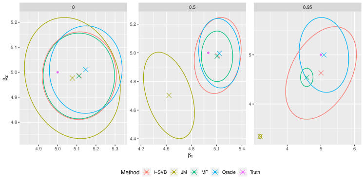
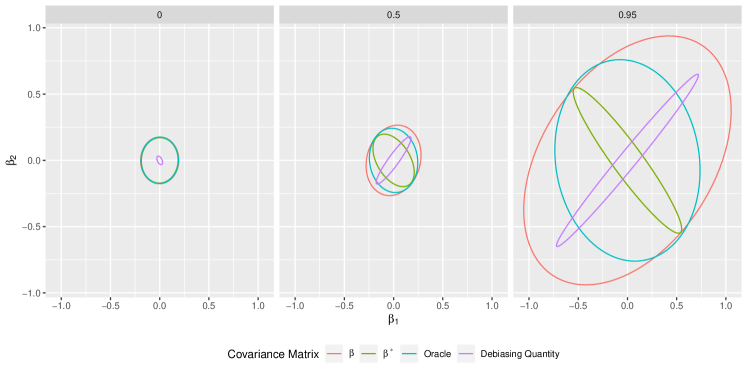
The above already shows the advantages of randomizing $\beta_{-k}$ in uncorrelated settings. We now turn to more correlated settings, again showing that the debiasing (and its randomization) plays a significant role. We provide analogous plots to Figures 1 and 2, but using the more heavily correlated structure where each row of the design is distributed as $X_{i\cdot}\sim\mathcal{N}_{p}(0,\Sigma_{\rho})$, where $[\Sigma_{\rho}]_{ij}=\rho$ if $i\neq j$ and is 1 otherwise, with results shown in Figures 4 and 5. Figure 4 presents a similar story to Figure 1, but in this case I-SVB is the only (non-Oracle) method to cover the truth in the most highly correlated scenario. Figure 5 shows that in this more correlated scenario, it is even more important to take into account the covariance structure of the debiasing, as the ellipse from $\beta_{1:2}^{*}$ is far too small; once the debiasing has taken place (which depends on $\beta_{-k}\sim\hat{Q}_{-k}$) the covariance structure of $\beta_{1:2}$ is better, though perhaps conservative.

Realisations of 2D credible regions Refer to caption

Figure 4: 95%-credible or confidence regions in three scenarios with design matrix rows $X_{i\cdot}\sim^{iid}\mathcal{N}_{p}(0,\Sigma_{\rho})$ for increasing values of $\rho$ given in the title of each facet. The interior of the ellipses represent the credible or confidence regions, the crosses mark their centering and the pink point is the true value of $(\beta_{1},\beta_{2})$. Each scenario has $n=200,p=400,k=2,s_{0}=10$ and $\beta^{0}_{i}=5$.

Covariance structure of the components of $\beta_{1:2}$ Refer to caption

Figure 5: Structure of the 95%-credible regions given by the covariance matrices of $\beta_{1:2}$, $\beta_{1:2}^{*}$, the Oracle, and the debiasing quantity ($(X_{1:2}^{T}X_{1:2})^{-1}X_{1:2}^{T}X_{-2}\beta_{-2}$) with design matrix rows $X_{i\cdot}\sim^{iid}\mathcal{N}_{p}(0,\Sigma_{\rho})$ for increasing values of $\rho$ given in the title of each facet. Each scenario has $n=200,p=400,k=2,s_{0}=10$ and $\beta^{0}_{i}=5$.

8.3 Additional simulations

Tables 6 and 7 show the performance of the various methods in some additional scenarios, where again the correlation structure between features is given by $\Sigma_{\rho}$. The discussion of these results is largely the same as that presented in Section 4; the I-SVB method delivers consistent uncertainty quantification in difficult scenarios where other methods struggle.

Scenario $(n,p,s_{0},\beta_{1}^{0},\beta_{j}^{0},\rho,\sigma^{2})$ Method Cov. MAE Length Time
$(vii)$ I-SVB 0.964 0.056 $\pm$ 0.041 0.281 $\pm$ 0.016 0.370 $\pm$ 0.127
$(200,800,3,\log n,\log n,0,1)$ MF 0.968 0.056 $\pm$ 0.041 0.279 $\pm$ 0.013 0.223 $\pm$ 0.092
ZZ 0.952 0.062 $\pm$ 0.046 0.293 $\pm$ 0.039 0.479 $\pm$ 0.153
JM 1.000 0.070 ± 0.053 0.483 ± 0.025 2.451 ± 0.203
$(viii)$ I-SVB 0.946 0.056 $\pm$ 0.045 0.286 $\pm$ 0.017 0.397 $\pm$ 0.135
$(200,800,10,\log n,\log n,0,1)$ MF 0.928 0.056 $\pm$ 0.045 0.279 $\pm$ 0.014 0.250 $\pm$ 0.119
ZZ 0.880 0.074 $\pm$ 0.059 0.295 $\pm$ 0.061 0.511 $\pm$ 0.161
JM 1.000 0.078 ± 0.058 0.498 ± 0.029 2.547 ± 0.291
$(ix)$ I-SVB 0.926 0.045 $\pm$ 0.034 0.203 $\pm$ 0.009 1.299 $\pm$ 0.238
$(400,1500,32,\mathcal{N}(0,1),\mathcal{N}(0,1),0,1)$ MF 0.818 0.059 $\pm$ 0.052 0.196 $\pm$ 0.007 0.688 $\pm$ 0.137
ZZ 0.822 0.059 $\pm$ 0.045 0.201 $\pm$ 0.012 1.396 $\pm$ 0.259
JM 0.724 0.145 ± 0.105 0.369 ± 0.015 17.77 ± 1.712
$(x)$ I-SVB 0.982 0.101 $\pm$ 0.075 0.595 $\pm$ 0.054 0.295 $\pm$ 0.091
$(100,1000,3,\log n,\log n,0.5,1)$ MF 0.896 0.097 $\pm$ 0.071 0.395 $\pm$ 0.028 0.273 $\pm$ 0.116
ZZ 0.948 0.152 $\pm$ 0.115 0.845 $\pm$ 0.603 0.324 $\pm$ 0.122
JM 0.960 0.231 ± 0.149 0.962 ± 0.11 1.718 ± 0.202
$(xi)$ I-SVB 0.986 0.069 $\pm$ 0.049 0.413 $\pm$ 0.032 0.359 $\pm$ 0.089
$(200,800,3,\log n,\log n,0.5,1)$ MF 0.914 0.067 $\pm$ 0.049 0.278 $\pm$ 0.014 0.261 $\pm$ 0.084
ZZ 0.978 0.084 $\pm$ 0.063 0.475 $\pm$ 0.078 0.530 $\pm$ 0.130
JM 0.976 0.131 ± 0.085 0.630 ± 0.063 3.863 ± 0.49
Table 6: Assessing the performance of the uncertainty quantification provided by each method in 5 additional scenarios. Highlighted in bold are the smallest interval length, subject to coverage being larger than 0.85, and the smallest MAE.
Scenario $(n,p,s_{0},\beta_{1}^{0},\beta_{j}^{0},\rho,\sigma^{2})$ Method Cov. MAE Length Time
$(xii)$ I-SVB 0.830 0.353 ± 0.272 1.349 ± 0.391 0.339 ± 0.112
$(100,1000,3,\log n,\log n,0,16)$ MF 0.802 0.391 ± 0.290 1.302 ± 0.399 0.228 ± 0.103
ZZ 0.766 0.468 ± 0.338 1.579 ± 1.185 0.296 ± 0.081
JM 0.924 0.596 ± 0.342 2.870 ± 0.854 1.636 ± 0.219
$(xiii)$ I-SVB 0.956 0.054 ± 0.042 0.281 ± 0.017 0.349 ± 0.083
$(200,1000,5,0,\log n,0,1)$ MF 1.000 0.000 ± 0.000 0.272 ± 0.014 0.211 ± 0.066
ZZ 0.976 0.049 ± 0.038 0.295 ± 0.048 0.434 ± 0.103
JM 1.000 0.041 ± 0.035 0.511 ± 0.028 2.980 ± 0.243
$(xiv)$ I-SVB 0.928 0.058 ± 0.045 0.283 ± 0.017 0.389 ± 0.092
$(200,1000,10,1,\log n,0,1)$ MF 0.930 0.058 ± 0.045 0.277 ± 0.014 0.238 ± 0.075
ZZ 0.854 0.082 ± 0.062 0.292 ± 0.036 0.469 ± 0.108
JM 0.974 0.092 ± 0.069 0.531 ± 0.032 3.237 ± 0.246
$(xv)$ I-SVB 0.962 0.037 ± 0.025 0.177 ± 0.007 1.157 ± 0.245
$(500,1000,10,\mathcal{U}(-5,5),\mathcal{U}(-5,5),0,1)$ MF 0.952 0.039 ± 0.030 0.176 ± 0.005 0.434 ± 0.140
ZZ 0.946 0.041 ± 0.027 0.178 ± 0.008 1.407 ± 0.343
JM 0.574 0.136 ± 0.113 0.267 ± 0.011 25.371 ± 7.692
$(xvi)$ I-SVB 0.986 0.101 ± 0.304 0.598 ± 0.124 0.978 ± 0.242
$(200,1000,10,1,\log n,0.5,1)$ MF 0.638 0.314 ± 0.466 0.276 ± 0.014 2.032 ± 0.587
ZZ 0.952 0.095 ± 0.074 0.482 ± 0.087 0.610 ± 0.079
JM 0.312 1.813 ± 1.359 1.496 ± 0.13 14.73 ± 1.267
Table 7: Assessing the performance of the uncertainty quantification provided by each method in 5 additional scenarios. Highlighted in bold are the smallest interval length, subject to coverage being larger than 0.85, and the smallest MAE.

9 Design matrix conditions

We provide here some further discussion to help understand the conditions on the design matrix required by our theoretical results. Our Bernstein-von Mises results in Section 3 require conditions on the compatibility constants of the transformed matrix $\check{W}$ in (6) rather than the original design $X$, which has been extensively studied in the literature [7]. The next lemma shows how one can relate these.

Lemma 4.

For any $S\subset\{1,\dots,p\}$ with $|S|>1$,

$$\phi^{\check{W}}(S\backslash\{1\})\geq\sqrt{1-\frac{1}{|S|}}\phi^{X}(S)-\frac{\|X_{1}\|_{2}}{\|\check{W}\|}\sqrt{|S|}\max_{i\geq 2}|\gamma_{i}|.$$

Furthermore, for any $s\in\{1,\dots,p\}$,

$$\tilde{\phi}^{\check{W}}(s-1)\geq\tilde{\phi}^{X}(s)-\frac{\|X_{1}\|_{2}}{\|\check{W}\|}\sqrt{s}\max_{i\geq 2}|\gamma_{i}|.$$

In particular, if (19) is satisfied, then

$$\phi^{\check{W}}(S\backslash\{1\})\geq\sqrt{1-\frac{1}{|S|}}\phi^{X}(S)-o(1)\quad\textrm{and}\quad\tilde{\phi}^{\check{W}}(s-1)\geq\tilde{\phi}^{X}(s)-o(1).$$
Proof of Lemma 4.

For the first statement, write $S_{*}=S\backslash\{1\}$. Observe that, for any $\beta\in\mathbb{R}^{p-1}$,

$\displaystyle\|\check{W}\beta\|_{2}$ $\displaystyle=\left\|X\left[\begin{matrix}0\\ \beta\end{matrix}\right]-X_{1}\sum_{i\geq 2}\gamma_{i}\beta_{i}\right\|_{2}\geq\left\|X\left[\begin{matrix}0\\ \beta\end{matrix}\right]\right\|_{2}-\|X_{1}\|_{2}\left|\sum_{i\geq 2}\gamma_{i}\beta_{i}\right|$ $\displaystyle\geq\left\|X\left[\begin{matrix}0\\ \beta\end{matrix}\right]\right\|_{2}-\|X_{1}\|_{2}\|\beta\|_{1}\max_{i\geq 2}|\gamma_{i}|.$ (37)

Then we have,

$\displaystyle\phi^{\check{W}}(S_{*})$ $\displaystyle=\inf_{\|\beta_{S_{*}^{C}}\|_{1}\leq 7\|\beta_{S_{*}}\|_{1}}\frac{\sqrt{|S_{*}|}\|\check{W}\beta\|_{2}}{\|\check{W}\|\|\beta_{S_{*}}\|_{1}}\geq\inf_{\|\beta_{S_{*}^{C}}\|_{1}\leq 7\|\beta_{S_{*}}\|_{1}}\frac{\sqrt{|S_{*}|}\left[\left\|X\left[\begin{matrix}0\\ \beta\end{matrix}\right]\right\|_{2}-\|X_{1}\|_{2}\|\beta\|_{1}\max_{i\geq 2}|\gamma_{i}|\right]}{\|\check{W}\|\|\beta_{S_{*}}\|_{1}}$
$\displaystyle\geq\inf_{\|\beta_{S_{*}^{C}}\|_{1}\leq 7\|\beta_{S_{*}}\|_{1}}\frac{\sqrt{|S_{*}|}\left\|X\left[\begin{matrix}0\\ \beta\end{matrix}\right]\right\|_{2}}{\|\check{W}\|\|\beta_{S_{*}}\|_{1}}-\frac{\sqrt{|S_{*}|}\|X_{1}\|_{2}\|\beta\|_{1}\max_{i\geq 2}|\gamma_{i}|}{\|\check{W}\|\|\beta_{S_{*}}\|_{1}}.$

Now, when $\|\beta_{S_{*}^{C}}\|_{1}\leq 7\|\beta_{S_{*}}\|_{1}$ we have $\|\beta\|_{1}/\|\beta_{S_{*}}\|_{1}\leq 8$, so the second term is bounded below by $-\frac{\|X_{1}\|_{2}}{\|\check{W}\|}\sqrt{|S_{*}|}\max_{i\geq 2}|\gamma_{i}|=-\frac{\|X_{1}\|_{2}}{\|\check{W}\|}\sqrt{|S_{*}|}\max_{i\geq 2}|\gamma_{i}|$. For the first term we have

$\displaystyle\inf_{\|\beta_{S_{*}^{C}}\|_{1}\leq 7\|\beta_{S_{*}}\|_{1}}\frac{\sqrt{|S_{*}|}\left\|X\left[\begin{matrix}0\\ \beta\end{matrix}\right]\right\|_{2}}{\|\check{W}\|\|\beta_{S_{*}}\|_{1}}$ $\displaystyle\geq\sqrt{1-\frac{1}{|S|}}\inf_{\|\beta^{\prime}_{S^{C}}\|_{1}\leq 7\|\beta^{\prime}_{S}\|_{1}}\frac{\sqrt{|S|}\left\|X\beta^{\prime}\right\|_{2}}{\|X\|\|\beta^{\prime}_{S}\|_{1}}$
$\displaystyle=\sqrt{1-\frac{1}{|S|}}\phi^{X}(S).$

For the second statement, write $s_{*}=s-1$. Once again using Equation (37), we have

$\displaystyle\tilde{\phi}^{\check{W}}(s_{*})$ $\displaystyle=\inf_{0\neq|S_{\beta}|\leq s_{*}}\frac{\|\check{W}\beta\|_{2}}{\|\check{W}\|\|\beta\|_{2}}\geq\inf_{0\neq|S_{\beta}|\leq s_{*}}\frac{\left[\left\|X\left[\begin{matrix}0\\ \beta\end{matrix}\right]\right\|_{2}-\|X_{1}\|_{2}\|\beta\|_{1}\max_{i\geq 2}|\gamma_{i}|\right]}{\|\check{W}\|\|\beta\|_{2}}$
$\displaystyle\geq\inf_{0\neq|S_{\beta}|\leq s_{*}}\frac{\left\|X\left[\begin{matrix}0\\ \beta\end{matrix}\right]\right\|_{2}}{\|\check{W}\|\|\beta\|_{2}}-\frac{\|X_{1}\|_{2}\|\beta\|_{1}\max_{i\geq 2}|\gamma_{i}|}{\|\check{W}\|\|\beta\|_{2}}.$

Now, when $0\neq|S_{\beta}|\leq s_{*}$ we have $\|\beta\|_{1}/\|\beta\|_{2}\leq\sqrt{s_{*}}$, so the second term is bounded below by $-\frac{\|X_{1}\|_{2}}{\|\check{W}\|}\sqrt{s_{*}}\max_{i\geq 2}|\gamma_{i}|=-\frac{\|X_{1}\|_{2}}{\|\check{W}\|}\sqrt{s_{*}}\max_{i\geq 2}|\gamma_{i}|$. For the first term we have,

$\displaystyle\inf_{0\neq|S_{\beta}|\leq s_{*}}\frac{\left\|X\left[\begin{matrix}0\\ \beta\end{matrix}\right]\right\|_{2}}{\|\check{W}\|\|\beta\|_{2}}$ $\displaystyle\geq\inf_{0\neq|S_{\beta^{\prime}}|\leq s}\frac{\left\|X\beta^{\prime}\right\|_{2}}{\|X\|\|\beta^{\prime}\|_{2}}=\phi^{X}(s).$

Lemma 4 shows that if (19) holds, then the compatibility constants for $\check{W}$ can be bounded from below by those for $X$, which is a much more commonly studied problem (e.g. Section D of [35]).

A related (but stronger) notion is the mutual coherence of $X$, given by

$$mc(X)=\max_{1\leq i\neq j\leq p}\frac{|X_{i}^{T}X_{j}|}{\|X_{i}\|_{2}\|X_{j}\|_{2}}.$$

Lemma 1 of [12] allows one to bound the compatibility numbers of $X$ from below if one has control of the mutual coherence via the following inqualities

$$\phi(S)^{2}\geq\bar{\phi}(1)^{2}-15\;|S|\;mc(X),\qquad\tilde{\phi}(s)^{2}\geq\bar{\phi}(1)^{2}-s\;mc(X),$$

where $\bar{\phi}(1)=\min_{i}\|X_{i}\|_{2}/\|X\|$ is typically bounded away from 0. We can relate the first quantity in our ‘no-bias’ condition (19) to the mutual coherence.

Lemma 5.

We have

$\displaystyle\frac{\|X_{1}\|_{2}\max_{i=2,\dots,p}|\gamma_{i}|}{\max_{i=2,\dots,p}\|(I-H)X_{i}\|_{2}}=\frac{\max_{i=2,\dots,p}\|HX_{i}\|_{2}}{\max_{i=2,\dots,p}\|(I-H)X_{i}\|_{2}}\leq\frac{mc(X)}{1-mc(X)}.$
Proof.

We begin with

$\displaystyle\left[\frac{\max_{i=2,\dots,p}\|HX_{i}\|_{2}}{\max_{i=2,\dots,p}\|(I-H)X_{i}\|_{2}}\right]^{2}\leq\left[\max_{i=2,\dots,p}\frac{\|HX_{i}\|_{2}}{\|(I-H)X_{i}\|_{2}}\right]^{2}=\max_{i=2,\dots,p}\frac{\|HX_{i}\|^{2}_{2}}{\|X_{i}\|^{2}_{2}-\|HX_{i}\|_{2}^{2}}.$

As $\|HX_{i}\|_{2}^{2}=(X_{i}^{T}X_{1})^{2}/\|X_{1}\|_{2}^{2}$,

$\displaystyle\max_{i=2,\dots,p}\frac{\|HX_{i}\|^{2}_{2}}{\|X_{i}\|^{2}_{2}-\|HX_{i}\|_{2}^{2}}$ $\displaystyle=\max_{i=2,\dots,p}\frac{(X_{i}^{T}X_{1})^{2}/\|X_{1}\|_{2}^{2}}{\|X_{i}\|^{2}_{2}-(X_{i}^{T}X_{1})^{2}/\|X_{1}\|_{2}^{2}}$
$\displaystyle=\max_{i=2,\dots,p}\frac{(X_{i}^{T}X_{1})^{2}/\|X_{1}\|_{2}^{2}\|X_{i}\|_{2}^{2}}{1-(X_{i}^{T}X_{1})^{2}/\|X_{1}\|_{2}^{2}\|X_{i}\|_{2}^{2}}$
$\displaystyle=\frac{\max_{i=2,\dots,p}(X_{i}^{T}X_{1})^{2}/\|X_{1}\|_{2}^{2}\|X_{i}\|_{2}^{2}}{1-\max_{i=2,\dots,p}(X_{i}^{T}X_{1})^{2}/\|X_{1}\|_{2}^{2}\|X_{i}\|_{2}^{2}},$

since the function $x\mapsto x/(1-x)$ is increasing. We now define $mc_{1}(X):=\max_{i=2,\dots,p}(X_{i}^{T}X_{1})/\|X_{1}\|_{2}\|X_{i}\|_{2}\leq mc(X)$, so that

$$\left[\frac{\max_{i=2,\dots,p}\|HX_{i}\|_{2}}{\max_{i=2,\dots,p}\|(I-H)X_{i}\|_{2}}\right]^{2}\leq\frac{mc_{1}(X)^{2}}{1-mc_{1}(X)^{2}}\leq\frac{mc(X)^{2}}{1-mc(X)^{2}}\leq\left[\frac{mc(X)}{1-mc(X)}\right]^{2}$$

since $x\mapsto\frac{x^{2}}{1-x^{2}}$ is increasing on $[0,1]$. Taking the square root of both sides completes the proof. ∎

If the entries of the design matrix $X_{ij}$ are i.i.d. with either $|X_{ij}|\leq C$ and $\log p=o(n)$ or $Ee^{t_{0}|X_{ij}|^{\alpha}}<\infty$ for some $\alpha,t_{0}>0$ and $\log p=o\left(n^{\frac{\alpha}{4+\alpha}}\right)$, then Theorems 1 and 2 of [9] give that $\sqrt{\frac{n}{\log p}}mc(X)\xrightarrow{P}2$ as $n\rightarrow\infty$. The compatibility numbers are then bounded away from 0 with probability 1 asymptotically for models of size $s_{0}=o(\sqrt{n/\log p})$. In addition, using Lemma 5, our ‘no-bias’ condition (19) is satisfied for models of size $s_{0}=o\left(\sqrt{n}/\log p\right)$.

As a concrete example to illustrate our conditions, we consider the case of the i.i.d. random design matrix $X\sim^{iid}\mathcal{N}(0,1)$. One can check that if the truth is sparse enough, then the conditions required in Theorem 1 hold with probability tending to 1.

Corollary 5.

Suppose that $\log p=o(n^{1/3})$ and $\beta^{0}\in\mathbb{R}^{p}$ is $s_{0}$-sparse with $s_{0}=o(\sqrt{n}/\log p)$. Consider the prior (5) with $\nu$ satisfying (4), $\lambda$ satisfying $2\frac{\sqrt{n-1}}{p-1}\leq\lambda\leq\,2\frac{\sqrt{(n-1)\log(p-1)}}{s_{0}}$ and $g$ is $c$-Lipschitz with $c=o(\sqrt{n})$. Then the semiparametric BvM holds for $\hat{Q}_{1}$.

Proof of Corollary 5.

Since the $X_{ij}\sim^{iid}\mathcal{N}(0,1)$ and $P^{T}P=I_{n-1}$, we have that the $\check{W}_{ij}$ are also i.i.d. $\mathcal{N}(0,1)$ and therefore the compatibility conditions can be verified using results on the compatibility of Gaussian matrices. More precisely, since $\log p=o(n^{1/3})$ and $s_{0}=o\left(\sqrt{n/\log p}\right)$, the compatibility numbers are bounded away from 0 on an event of probability 1 asymptotically as discussed above. Similarly, since $s_{0}=o(\sqrt{n}/\log p)$, condition (19) is satisfied with probability 1 asymptotically.

Since the $X_{ij}$ are i.i.d. $\mathcal{N}(0,1)$ and the $\check{W}_{ij}$ are also i.i.d. $\mathcal{N}(0,1)$, we have $\|X_{1}\|_{2}=\sqrt{n}(1+o_{P}(1))$ and $\|\check{W}\|=\sqrt{n-1}(1+o_{P}(1))$. Therefore, by the assumptions on $\lambda$ and $c$, the conditions required on $\lambda$ and $c$ in the deterministic case are satisfied on an event of probability 1 asymptotically. ∎

10 A connection to a larger variational class

As discussed in the introduction, our method can be viewed more generally as placing a rough MF variational approximation on the high-dimensional nuisance parameters $\beta_{-1}$ and then carefully modelling the conditional distribution $\beta_{1}|\beta_{-1}$. We now make this link precise, showing that our variational approximation (11) corresponds to the KL-minimizer of such a variational family. More precisely, define the set of conditional densities:

$$\mathcal{D}=\left\{q:\mathbb{R}\times\mathbb{R}^{p-1}\rightarrow[0,\infty):\;q(\cdot|\beta_{-1})\;\text{is a density with respect to Lebesgue measure for all }\beta_{-1}\in\mathbb{R}^{p-1}\right\},$$

and the variational class

$$\mathcal{V}=\left\{q(\beta_{1}|\beta_{-1})d\beta_{1}dQ_{-1}(\beta_{-1}):\ q\in\mathcal{D}\,,\,Q_{-1}\in\mathcal{Q}_{-1}\right\}.$$

In Lemma 6, we show that the KL-minimizer between $\mathcal{V}$ and the posterior is given by $q=\pi(\cdot|\beta_{-1},Y)$ with $\pi(\cdot|\beta_{-1},Y)$ being the conditional distribution of $\beta_{1}|\beta_{-1}$ under the posterior, and $Q_{-1}=\hat{Q}_{-1}$. By rewriting the distribution (11) in term of a distribution on $\beta_{-1}$ and a conditional distribution of $\beta_{1}|\beta_{-1}$ , one can see that this minimizer is exactly the approximation (11).

Lemma 6.

For any $V=V(q,Q_{-1})$ in $\mathcal{V}$,

$\displaystyle\operatorname{KL}(V\|\Pi(\cdot|Y))=\operatorname{KL}(Q_{-1}\|\Pi_{-1}(\cdot|Y))+\int_{\mathbb{R}^{p-1}}\operatorname{KL}(q(\cdot|\beta_{-1})\|\pi(\cdot|\beta_{-1},Y))dQ_{-1}.$

Consequently,

$\displaystyle\operatorname*{arg\,min}_{V\in\mathcal{V}}\operatorname{KL}(V,\Pi(\cdot|Y))=V(\pi(\cdot|\beta_{-1},Y),\hat{Q}_{-1}).$
Proof of Lemma 6.

We prove the first assertion. Let $V=V(q,Q_{-1})\in\mathcal{V}$ with $Q_{-1}$ being absolutely continuous with respect to $\Pi_{-1}(\cdot|Y)$, otherwise the result is immediate. We have that

$\displaystyle dV(\beta)$ $\displaystyle=q(\beta_{1}|\beta_{-1})d\beta_{1}\frac{dQ_{-1}}{d\Pi_{-1}(\cdot|Y)}(\beta_{-1})d\Pi_{-1}(\beta_{-1}|Y)$
$\displaystyle=\frac{q(\beta_{1}|\beta_{-1})}{\pi(\beta_{1}|\beta_{-1},Y)}\pi(\beta_{1}|\beta_{-1},Y)d\beta_{1}\frac{dQ_{-1}}{d\Pi_{-1}(\cdot|Y)}(\beta_{-1})d\Pi_{-1}(\beta_{-1}|Y)$
$\displaystyle=\frac{q(\beta_{1}|\beta_{-1})}{\pi(\beta_{1}|\beta_{-1},Y)}\frac{dQ_{-1}}{d\Pi_{-1}(\cdot|Y)}(\beta_{-1})d\Pi(\beta|Y).$

Consequently, $V$ is absolutely continous with respect to $\Pi(\cdot|Y)$ and

$\displaystyle\operatorname{KL}(V||\Pi(\cdot|Y))$ $\displaystyle=\int\log(\frac{q(\beta_{1}|\beta_{-1})}{\pi(\beta_{1}|\beta_{-1},Y)}\frac{dQ_{-1}}{d\Pi_{-1}(\cdot|Y)}(\beta_{-1}))dV(\beta)$
$\displaystyle=\int\log(\frac{q(\beta_{1}|\beta_{-1})}{\pi(\beta_{1}|\beta_{-1},Y)})dV(\beta)+\int\log(\frac{dQ_{-1}}{d\Pi_{-1}(\cdot|Y)}(\beta_{-1}))dV(\beta)$
$\displaystyle=\int_{\mathbb{R}^{p-1}}\int_{\mathbb{R}}\log(\frac{q(\beta_{1}|\beta_{-1})}{\pi(\beta_{1}|\beta_{-1},Y)})q(\beta_{1}|\beta_{-1})d\beta_{1}dQ_{-1}(\beta_{-1})+\int_{\mathbb{R}^{p-1}}\log(\frac{dQ_{-1}}{d\Pi_{-1}(\cdot|Y)})dQ_{-1}$
$\displaystyle=\int_{\mathbb{R}^{p-1}}\operatorname{KL}(q(\cdot|\beta_{-1})\|\pi(\cdot|\beta_{-1},Y))dQ_{-1}+\operatorname{KL}(Q_{-1}||\Pi_{-1}(\cdot|Y)).$

The second assertion can be easily deduced form the first assertion. ∎

References

  • Alquier and Ridgway [2020] Pierre Alquier and James Ridgway. Concentration of tempered posteriors and of their variational approximations. Ann. Statist., 48(3):1475–1497, 2020.
  • Bai et al. [2022] Ray Bai, Gemma Moran, Joseph Antonelli, Yong Chen, and Mary Regina Boland. Spike-and-slab group lassos for grouped regression and sparse generalized additive models. J. Am. Statist. Ass., pages 1–41, 2022.
  • Banerjee et al. [2021] Sayantan Banerjee, Ismaël Castillo, and Subhashis Ghosal. Bayesian inference in high-dimensional models. 2021. Book chapter to appear in Springer volume on data science, Preprint arXiv:2101.04491.
  • Bierkens et al. [2023] Joris Bierkens, Sebastiano Grazzi, Frank van der Meulen, and Moritz Schauer. Sticky PDMP samplers for sparse and local inference problems. Stat. Comput., 33(1):Paper No. 8, 31, 2023.
  • Bishop [2006] Christopher M. Bishop. Pattern recognition and machine learning. Information Science and Statistics. Springer, New York, 2006.
  • Blei et al. [2017] David M. Blei, Alp Kucukelbir, and Jon D. McAuliffe. Variational inference: a review for statisticians. J. Amer. Statist. Assoc., 112(518):859–877, 2017.
  • Bühlmann and van de Geer [2011] Peter Bühlmann and Sara van de Geer. Statistics for high-dimensional data. Springer Series in Statistics. Springer, Heidelberg, 2011. Methods, theory and applications.
  • Bühlmann et al. [2014] Peter Bühlmann, Markus Kalisch, and Lukas Meier. High-dimensional statistics with a view toward applications in biology. Annual Review of Statistics and Its Application, 1(Volume 1, 2014):255–278, 2014.
  • Cai and Jiang [2011] T. Tony Cai and Tiefeng Jiang. Limiting laws of coherence of random matrices with applications to testing covariance structure and construction of compressed sensing matrices. Ann. Statist., 39(3):1496 – 1525, 2011.
  • Carbonetto and Stephens [2012] Peter Carbonetto and Matthew Stephens. Scalable variational inference for Bayesian variable selection in regression, and its accuracy in genetic association studies. Bayesian Anal., 7(1):73–107, 2012.
  • Castillo and Rousseau [2015] Ismaël Castillo and Judith Rousseau. A Bernstein–von Mises Theorem for smooth functionals in semiparametric models. Ann. Statist., 43(6), 2015. doi: 10.1214/15-aos1336.
  • Castillo et al. [2015] Ismaël Castillo, Johannes Schmidt-Hieber, and Aad van der Vaart. Bayesian linear regression with sparse priors. Ann. Statist., 43(5):1986 – 2018, 2015.
  • Castillo and van der Vaart [2012] Ismaël Castillo and Aad van der Vaart. Needles and straw in a haystack: Posterior concentration for possibly sparse sequences. Ann. Statist., 40(4), 2012. doi: 10.1214/12-aos1029.
  • Chae et al. [2019] Minwoo Chae, Lizhen Lin, and David B. Dunson. Bayesian sparse linear regression with unknown symmetric error. Inf. Inference, 8(3):621–653, 2019.
  • Clara et al. [2020] Gabriel Clara, Botond Szabo, and Kolyan Ray. sparsevb: spike and slab variational Bayes for linear and logistic regression, 2020. R package version 1.0.
  • Dudley [2002] R. M. Dudley. Real analysis and probability, volume 74 of Cambridge Studies in Advanced Mathematics. Cambridge University Press, Cambridge, 2002. Revised reprint of the 1989 original.
  • Fasano et al. [2022] Augusto Fasano, Daniele Durante, and Giacomo Zanella. Scalable and accurate variational Bayes for high-dimensional binary regression models. Biometrika, 109(4):901–919, 2022.
  • Gao et al. [2020] Chao Gao, Aad W. van der Vaart, and Harrison H. Zhou. A general framework for Bayes structured linear models. Ann. Statist., 48(5):2848 – 2878, 2020.
  • Goplerud [2022] Max Goplerud. Fast and accurate estimation of non-nested binomial hierarchical models using variational inference. Bayesian Anal., 17(2):623–650, 2022.
  • Goplerud et al. [2023] Max Goplerud, Omiros Papaspiliopoulos, and Giacomo Zanella. Partially factorized variational inference for high-dimensional mixed models, 2023. arXiv preprint: 2312.13148.
  • Griffin et al. [2021] J. E. Griffin, K. G. Łatuszyński, and M. F. J. Steel. In search of lost mixing time: adaptive Markov chain Monte Carlo schemes for Bayesian variable selection with very large $p$. Biometrika, 108(1):53–69, 2021.
  • Hoffman and Blei [2015] Matthew Hoffman and David Blei. Stochastic structured variational inference. In Artificial Intelligence and Statistics, pages 361–369. PMLR, 2015.
  • Ishwaran and Rao [2005] Hemant Ishwaran and J. Sunil Rao. Spike and slab variable selection: Frequentist and Bayesian strategies. Ann. Statist., 33(2):730–773, 2005.
  • Janková and van de Geer [2018] Jana Janková and Sara van de Geer. Semiparametric efficiency bounds for high-dimensional models. Ann. Statist., 46(5):2336–2359, 2018.
  • Javanmard and Montanari [2014] Adel Javanmard and Andrea Montanari. Confidence intervals and hypothesis testing for high-dimensional regression. J. Mach. Learn. Res., 15(82):2869–2909, 2014.
  • Javanmard and Montanari [2018] Adel Javanmard and Andrea Montanari. Debiasing the Lasso: optimal sample size for Gaussian designs. Ann. Statist., 46(6A):2593–2622, 2018.
  • Johnson and Rossell [2010] Valen E. Johnson and David Rossell. On the use of non-local prior densities in Bayesian hypothesis tests. J. R. Statist. Soc. B, 72(2):143–170, 2010.
  • Komodromos et al. [2022] Michael Komodromos, Eric O Aboagye, Marina Evangelou, Sarah Filippi, and Kolyan Ray. Variational Bayes for high-dimensional proportional hazards models with applications within gene expression. Bioinformatics, 38(16):3918–3926, 2022.
  • Komodromos et al. [2023] Michael Komodromos, Marina Evangelou, Sarah Filippi, and Kolyan Ray. Group spike and slab variational Bayes, 2023. arXiv preprint: 2309.10378.
  • Logsdon et al. [2010] Benjamin A Logsdon, Gabriel E Hoffman, and Jason G Mezey. A variational Bayes algorithm for fast and accurate multiple locus genome-wide association analysis. BMC bioinformatics, 11:1–13, 2010.
  • Martin et al. [2017] Ryan Martin, Raymond Mess, and Stephen G. Walker. Empirical Bayes posterior concentration in sparse high-dimensional linear models. Bernoulli, 23(3):1822–1847, 2017.
  • Menictas et al. [2023] Marianne Menictas, Gioia Di Credico, and Matt P. Wand. Streamlined variational inference for linear mixed models with crossed random effects. J. Comput. Graph. Statist., 32(1):99–115, 2023.
  • Nieman et al. [2023] Dennis Nieman, Botond Szabo, and Harry van Zanten. Uncertainty quantification for sparse spectral variational approximations in Gaussian process regression. Electron. J. Stat., 17(2):2250–2288, 2023.
  • Ormerod et al. [2017] John T. Ormerod, Chong You, and Samuel Müller. A variational Bayes approach to variable selection. Electron. J. Stat., 11(2):3549–3594, 2017.
  • Ray and Szabó [2022] Kolyan Ray and Botond Szabó. Variational Bayes for high-dimensional linear regression with sparse priors. J. Am. Statist. Ass., 117(539):1270–1281, 2022.
  • Ray et al. [2020] Kolyan Ray, Botond Szabo, and Gabriel Clara. Spike and slab variational Bayes for high dimensional logistic regression. In Advances in Neural Information Processing Systems, volume 33, pages 14423–14434, 2020.
  • Rivoirard and Rousseau [2012] Vincent Rivoirard and Judith Rousseau. Bernstein–von Mises theorem for linear functionals of the density. Ann. Statist., 40(3):1489 – 1523, 2012.
  • Tan [2021] Linda S. L. Tan. Use of model reparametrization to improve variational Bayes. J. R. Statist. Soc. B, 83(1):30–57, 2021.
  • Tan and Nott [2013] Linda S. L. Tan and David J. Nott. Variational inference for generalized linear mixed models using partially noncentered parametrizations. Statist. Sci., 28(2):168–188, 2013.
  • Tibshirani [1996] Robert Tibshirani. Regression shrinkage and selection via the lasso. J. R. Statist. Soc. B, 58(1):267–288, 1996.
  • Travis and Ray [2024] Luke Travis and Kolyan Ray. Pointwise uncertainty quantification for sparse variational Gaussian process regression with a brownian motion prior. In Advances in Neural Information Processing Systems, volume 36, 2024.
  • Vakili et al. [2022] Sattar Vakili, Jonathan Scarlett, Da-shan Shiu, and Alberto Bernacchia. Improved convergence rates for sparse approximation methods in kernel-based learning. In International Conference on Machine Learning, pages 21960–21983. PMLR, 2022.
  • van de Geer et al. [2014] Sara van de Geer, Peter Bühlmann, Ya’acov Ritov, and Ruben Dezeure. On asymptotically optimal confidence regions and tests for high-dimensional models. Ann. Statist., 42(3):1166 – 1202, 2014.
  • Wang and Blei [2019] Yixin Wang and David M. Blei. Frequentist consistency of variational Bayes. J. Am. Statist. Ass., 114(527):1147–1161, 2019.
  • Yang [2019] Dana Yang. Posterior asymptotic normality for an individual coordinate in high-dimensional linear regression. Electron. J. Stat., 13(2):3082 – 3094, 2019.
  • Yang et al. [2020] Yun Yang, Debdeep Pati, and Anirban Bhattacharya. $\alpha$-variational inference with statistical guarantees. Ann. Statist., 48(2):886–905, 2020.
  • Zhang and Zhang [2014] Cun-Hui Zhang and Stephanie S. Zhang. Confidence intervals for low dimensional parameters in high dimensional linear models. J. R. Statist. Soc. B, 76(1):217–242, 2014.
  • Zhang and Gao [2020] Fengshuo Zhang and Chao Gao. Convergence rates of variational posterior distributions. Ann. Statist., 48(4):2180–2207, 2020.
  • Zou [2006] Hui Zou. The adaptive lasso and its oracle properties. J. Am. Statist. Ass., 101(476):1418–1429, 2006.