Lindblad quantum dynamics from correlation functions of classical spin chains
Abstract
The Lindblad quantum master equation is one of the central approaches to the physics of open quantum systems. In particular, boundary driving enables the study of transport, where a steady state emerges in the long-time limit, which features a constant current and a characteristic density profile. While the Lindblad equation complements other approaches to transport in closed quantum systems, it has become clear that a connection between closed and open systems exists in certain cases. Here, we build on this connection for magnetization transport in the spin-1/2 XXZ chain with and without integrability-breaking perturbations. Specifically, we show that the time evolution of the open quantum system can be described on the basis of classical correlation functions, as generated by the Hamiltonian equations of motion for real vectors. By comparing to exact numerical simulations of the Lindblad equation, we demonstrate the accuracy of this description for a range of model parameters, but also point out counterexamples. While this agreement is an interesting physical observation, it also suggests that classical mechanics can be used to solve the Lindblad equation for comparatively large system sizes, which lie outside the possibilities of a quantum mechanical treatment.
I Introduction
Many-body quantum systems out of equilibrium can be studied in two complementary scenarios. Either, the system is closed and couples by no means to the rest of the world. Or, the system is open and explicitly couples to a bath, where the system-bath coupling can be weak or strong. Both scenarios are interesting and important by their own right and allow to address a large variety of questions in modern physics, ranging from fundamental questions in statistical mechanics to applied questions in material science. A central question in closed and open scenarios is the system’s evolution in the course of time and the existence and properties of steady states in the long-time limit [1, 2, 3, 4, 5]. The study of this particular question has seen remarkable progress in the past, due to experimental advances [6], fresh theoretical concepts like typicality of pure quantum states [7, 8, 9, 10, 11, 12, 13, 14, 15] and eigenstate thermalization [16, 17, 18], and the development of sophisticated numerical techniques [19, 20].
Within the diverse class of nonequilibrium processes, transport is a natural one for systems with one or more globally conserved quantities [21], like total energy, particle number, or magnetization. Transport is further a process which is relevant to both, closed and open situations. In an open situation, the system of actual interest can be coupled at its boundaries to two reservoirs at different temperatures or chemical potentials, such that transport is induced and a nonequilibrium steady state is usually established in the long-time limit [22, 23, 24]. In this steady state, the constant current and the form of the density profile yield information on the qualitative type of transport and also allow to determine quantitative values for transport coefficients [21]. A widely used strategy to describe such an open scenario is the Lindblad equation [25], which has its assets and drawbacks. On the one hand, the derivation of this equation from a microscopic system-bath model can be a nontrivial task in praxis [26, 27]. On the other hand, it is the most general form of a quantum master equation, which is local in time and maps any density matrix to a density matrix again. Furthermore, the structure of the Lindblad equation enables the application of well-suited numerical techniques. Here, one method is provided by the concept of stochastic unraveling [28, 29], which constructs the time evolution of the density matrix in Liouville space as the average over many pure-state trajectories in Hilbert space. An alternative method is given by matrix product states [30, 31, 23, 32], where entanglement growth is reduced because of dissipation.
In closed systems, a main approach is linear response theory, which predicts the behavior close to equilibrium in terms of correlation functions at equilibrium. While in the context of transport the current autocorrelation is a central object and enters the well-known Kubo formula [33], the transport behavior is also encoded in density-density correlations, which can be analyzed in real or momentum space and in the time or frequency domain. Even though the investigation of correlation functions has a long and fertile history, the concrete calculation for specific models can still be a challenging task in praxis. In particular, seemingly simple models like the integrable spin- XXZ chain have turned out to be notoriously difficult for both, analytical and numerical methods [21]. Models of interacting spins are valuable, because they are not only many-body quantum systems with rich phase diagrams, but also have a classical counterpart [34, 35, 36, 37, 38, 39, 40, 41, 42, 43, 44, 45, 46, 47, 48, 49, 50, 51, 52, 53, 54, 55, 56, 57, 58, 59, 60, 61], which corresponds to the limit of large spin quantum numbers . While the cases of and can in general not be expected to exhibit the same physics, it has been observed that their dynamics is similar for some examples [62, 63], qualitatively and also quantitatively. Such a similarity has been found for correlation functions in the XXZ chain in the limit of high temperatures [64, 65], where the low-energy excitations are less relevant [66].
In this paper, we also investigate to what extent the time evolution in a quantum system can be described on the basis of the dynamics in the classical counterpart. In contrast to previous works, which have been devoted to a comparison of the corresponding correlation functions in a closed scenario [64, 65], we intend to go a substantial step beyond. Specifically, we are going to compare the open quantum system to the closed classical system. For such a comparison, we obviously need a connection between the dynamics in open and closed scenarios [67, 68], which does not exist in general [69, 70, 71]. For the spin- chain, however, a connection has been recently suggested [72] for the case of small system-bath coupling and weak driving. Because this connection involves quantum correlation functions, we replace them by the corresponding classical ones. In this way, we can address the main question of our work: Is it possible to obtain Lindblad quantum dynamics from correlation functions of classical spin chains? To answer this question, we compare to exact numerical simulations of the Lindblad equation. While we observe a remarkably good agreement for a range of model parameters, we also point out counterexamples. This agreement further hints that classical mechanics can be used as a strategy to solve the Lindblad equation for large system sizes, which are not accessible in a quantum mechanical treatment. Such a classical strategy has been also discussed in other open quantum systems [73].
This paper is structured as follows: We introduce the open quantum system in Sec. II. Then, we discuss the connection between open and closed systems in Sec. III and the classical limit in Sec. IV. Next, we present our numerical results in Sec. V. We close with a summary and conclusion in Sec. VI. Further information can be found in the appendix.
II Open quantum system
Let us start by introducing the open quantum system considered throughout this work. We choose to describe this system by the Lindblad equation,
| (1) |
as the most general form of a quantum master equation, which is local in time and maps any density matrix to a density matrix again [25]. While the first term on the r.h.s. is coherent and describes the unitary time evolution w.r.t. to a given Hamiltonian , the second term on the r.h.s. is incoherent and describes the damping due to the presence of a bath. This damping reads
| (2) |
with Lindblad operators , non-negative rates , and the anticommutator .
Next, we define the Hamiltonian and a suitable set of Lindblad operators . Focusing first on , we choose the spin- XXZ chain [21],
| (3) |
where are the components of a spin- operator at site , is the number of sites, is the antiferromagnetic coupling constant, and is the anisotropy in direction. We assume periodic boundary conditions, , which are for our purposes more convenient than open boundary conditions, as discussed later.
Because the Hamiltonian in Eq. (3) is integrable for all possible values of the anisotropy , we additionally take into account an integrability-breaking perturbation. Our choice for such a perturbation are interactions between next-to-nearest sites,
| (4) |
where is the perturbation strength and, as before, we assume periodic boundary conditions.
For each of the Hamiltonians in Eqs. (3) and (4), the total magnetization is a strictly conserved quantity, . Thus, the transport of local magnetization is a meaningful question. The study of transport also motivates our choice of the Lindblad operators . Specifically, we make a simple but common choice [21],
| (5) | ||||
| (6) | ||||
| (7) | ||||
| (8) |
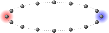
where is the system-bath coupling and is the driving strength. The local operators and act on the site and flip a spin up and down, respectively. The other operators and act in the same way on another site . To maximize the size of the bulk, we set and , as illustrated in Fig. 1. Due to the choice of the rates in Eqs. (5) - (8), net magnetization flows from the first bath into the system and from the system into the second bath, which leads to a nonequilibrium steady state in the long-time limit.
For this open quantum system, we are interested in the dynamics of local magnetization, which includes the steady-state profile on the one hand and its buildup in time on the other hand. Hence, we study the expectation value
| (9) |
which depends on the Hamiltonian , but also on the system-bath coupling and the driving strength . We focus on the case of small and . As initial condition, we use the ensemble
| (10) |
for high temperatures , which features a homogeneous profile of magnetization.
An exact analytical solution of the Lindblad equation, or an accurate approximation of it, can in general not be derived. Hence, one has to resort typically to numerical methods. In this context, standard exact diagonalization is particularly challenging, since the Liouville space (of dimension is substantially larger than the anyhow large Hilbert space (). Yet, the Lindblad form allows for stochastic unraveling [28, 29], which yields the time-dependent density matrix as the average over many pure-state trajectories. Additionally, simulations on the basis of matrix product states [30, 31, 23, 32] give access to systems of hundreds of spins, at least on time scales with a still low amount of entanglement.
In this work, we mostly rely on existing numerical data in the literature [72, 74], which we use later for a comparison to our approach on the basis of classical mechanics. Before we explain what we mean by classical mechanics, we need to discuss another concept, i.e., a connection between the dynamics in open and closed quantum systems.
III Connection between open and closed systems
In general, one can hardly expect a direct connection between the time evolution in open and closed quantum systems. For the specific scenario introduced in Sec. II, however, such a connection has been shown to exist, at least in certain cases [72]. This connection makes use of spatio-temporal correlation functions,
| (11) |
which are evaluated in the closed system at thermal equilibrium. For high temperatures , which we use from now on, they simplify to
| (12) |
Before we formulate the actual connection, it is useful to introduce a superposition of Eq. (12) with and Eq. (12) with ,
| (13) |
and then to define the more complex superposition
| (14) |
where are some amplitudes, are some times, and is the Heavyside function. Using this notation, we can eventually formulate the connection and express the nonequilibrium dynamics of the open system in Eq. (9) as [72]
| (15) |
where the sum runs over different time sequences . Here, a particular time sequence is generated by
| (16) |
where are random numbers drawn from a uniform distribution in the interval . The amplitudes are now given by
| (17) |
with
| (18) |
If , .
While the connection might look quite complicated at first sight, it is rather simple, especially since it expresses the nonequilibrium dynamics in the open system just as a superposition of equilibrium correlation functions in the closed system. As discussed in Ref. [72], such a connection cannot always hold and requires sufficiently small values of both, and . Furthermore, it assumes the absence of nondecaying edge modes, which can occur in a closed system with open boundary conditions [75, 76]. For this reason, we focus on periodic boundary conditions.
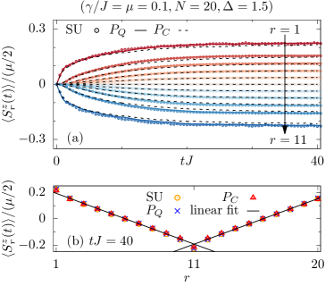
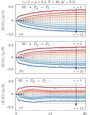
In Fig. 2, we illustrate the quality of the connection, by comparing the prediction on the r.h.s. of Eq. (15) to a simulation based on stochastic unraveling for the l.h.s. of Eq. (15). We do so for the model in Eq. (4) with , , , periodic boundary conditions, small coupling , and weak driving . For this set of parameters, the agreement between both sides is remarkable. While Fig. 2 shows existing data from the literature [72], it already depicts a prediction by the use of classical mechanics, as a main result of our work. This prediction is discussed in the following.
IV Classical limit
To introduce the classical limit of our models, let us consider an arbitrary spin quantum number . Then, the spin- operators fulfill the usual commutation relations, which read
| (19) |
with the Kronecker symbol and the antisymmetric Levi-Civita tensor . Here, we write explicitly, while it is otherwise set to unity. The classical counterpart of our models now results by taking the limit
| (20) |
In this limit, the commutation relations in Eq. (19) turn into the Poisson-bracket relations
| (21) |
for real and three-dimensional spin vectors of unit length, . The Hamilton operators and in Eqs. (3) and (4) become Hamilton functions, but apart from that look the same. The total magnetization is still strictly conserved, .
The Poisson-bracket relations in Eq. (21) also lead to Hamilton’s equations of motion,
| (22) |
Physically, these equations describe the precession of a spin around a magnetic field, which is generated by the interaction with the neighboring spins. Mathematically, they are a coupled set of nonlinear differential equations, which is nonintegrable by means of the Liouville-Arnold theorem, even for [77, 78]. Therefore, for nontrivial initial conditions, they have to be solved numerically, as we also do here. Throughout our work, we employ a fourth-order Runge-Kutta scheme with a time step , which is small enough to ensure that the total magnetization is well conserved during the time evolution.
Now, we come to the central objects in our work, i.e., the spatio-temporal correlation functions in the realm of classical mechanics. Focusing again on high temperatures , they read
| (23) |
where is the number of realizations for different initial conditions, which are randomly drawn from phase space. Formally, . In praxis, we average over as many realizations as , to ensure that the remaining stochastic fluctuations are low. The need for such an extensive averaging in the numerical simulations is kind of compensated by the fact that the phase space grows only linearly with , in contrast to the exponential growth of the Hilbert space. Due to this fact, we can particularly treat classical systems of quite large size , which lie outside the possibilities of a quantum mechanical treatment. Still, we also consider small to enable a comparison to quantum mechanics for the same size.
Eventually, coming back to the connection between the dynamics in open and closed systems, Eq. (15), the main idea is to replace the quantum correlation functions by the corresponding classical ones. When we do this strong simplification, the key question of our work is whether or not the time evolution in the open system can be still described accurately. To answer this question in a kind of fair way, we first need to rescale the classical time by a factor
| (24) |
which is and close to one. Then, we additionally need to rescale the initial value of the classical correlation (), since the one of the quantum correlation () is different. Apart from these rescalings, no further modifications are done and the dynamics as such is fully generated by Hamilton’s equation of motion.
V Results
V.1 Nearest-neighbor interactions
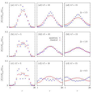
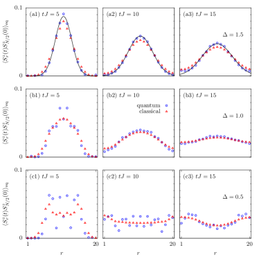
Next, we turn to our numerical simulations, with the central aim to scrutinize to what degree the open-system quantum dynamics can be described by an approach on the basis of classical mechanics. Because we rely on the connection in Eq. (15), where correlation functions in the closed system are the main ingredient, we start with comparing quantum and classical correlation functions in the closed scenario. We do so for the spin- XXZ chain in Eq. (4) with and . However, we also address the case of and later. The remaining parameters of the model are chosen to cover different quantum behaviors [21]: (a) diffusive behavior for , (b) superdiffusive behavior for , and (c) ballistic behavior for . While our calculation of quantum correlations uses the concept of dynamical quantum typicality in its standard formulation [14, 15], our calculation of classical correlations is done in the way as outlined above. Similar comparisons can be found in the literature [65].
In Fig. 3, we summarize the comparison, by showing the site dependence of quantum and classical correlations for different times. As visible in Fig. 3 (first and second row), there is a quite convincing agreement for and . While minor deviations occur at short times, the overall site dependence is similar for longer times, which indicates that diffusion as such is not a prerequisite. Less convincing is the comparison for . Still, quantum and classical correlations agree roughly and one might be tempted to conclude that the transport behavior is the same. However, the quantum case is well-known to be ballistic [21], while the classical case is likely diffusive, due to nonintegrability. Thus, the rough agreement reflects that the classical dynamics has still not reached the mean free path.
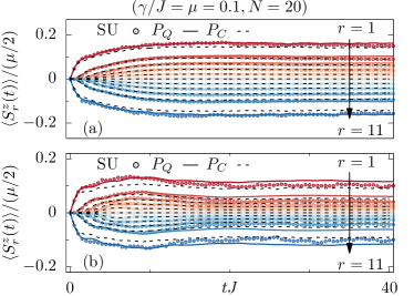
Using the correlations in Fig. 3, we now calculate the corresponding predictions for the time evolution of the open system, according to Eq. (15). In this calculation, we average over different time sequences, which is enough to obtain sufficiently smooth curves. As already advertised before, Fig. 2 illustrates for a convincing agreement with existing simulations [72] on the basis of stochastic unraveling. In Fig. 4, we also depict a comparison for and . While the agreement for is also good, some disagreement is visble for . Of course, one might expect this disagreement in view of the differences between quantum and classical correlations in Fig. 3 (third row). However, it should be noted that also the quantum prediction differs from the stochastic-unravling data. This deviation can be traced back to the fact that the ballistic quantum motion for partially violates the equilibration assumption, which underlies the derivation of Eq. (15).
V.2 Next-to-nearest-neighbor interactions
Now, we allow for interactions between next-to-nearest sites and specifically choose a value of . Naively, one might expect that the overall agreement is improved, because the quantum and classical model become both nonintegrable for and as a consequence should possess diffusion. However, this expectation turns out to be wrong.
In comparison to Fig. 3 for , the quantum and classical correlations in Fig. 5 for do not agree as well as before. While the agreement for is again convincing, deviations start to set in for . These deviations might be a signal that the quantum-classical correspondence eventually breaks down completely in the limit of very strong interactions. Yet, the correspondence is still satisfactory.
For in Fig. 5 (third row), the agreement turns out to be worst. While the quantum and classical case are both expected to exhibit diffusion, the quantum dynamics has not reached the mean free path, at least for the time scales considered. In contrast, the classical dynamics has reached the mean free path and already takes place in the hydrodynamic regime. Therefore, while transport might be qualitatively the same, it is quantitatively clearly different.
Using the correlations in Fig. 5, we again calculate the corresponding predictions for the time evolution of the open system. As can be seen, the quality of agreement in the closed system carries over to a similar quality in the open system. It is worth pointing out that the quantum prediction, in contrast to the classical prediction, is in excellent agreement with existing stochastic-unraveling data [74], for all values of .
V.3 Larger system sizes
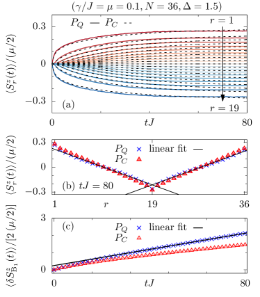
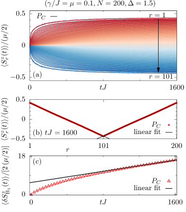
Next, we move forward to substantially larger system sizes. Here, stochastic unraveling is not feasible anymore and we cannot compare to corresponding data. Thus, we have to rely on a comparison between the quantum and classical predictions for the time evolution of the open system, as given in Eq. (15). We focus on the parameters and , which in our previous comparisons has turned out to be the best case. In Fig. 7, we depict results for , where the quantum prediction can still be carried out, due to existing data for correlations [72] from a calculation on a super computer. Apparently, the agreement between the two predictions for is as convincing as for considered before, which indicates that system size as such is not important for the accuracy of a classical treatment.
In Fig. 7 (c), we additionally depict a quantity, which we have not discussed so far. This quantity is the induced magnetization by the first bath, , as defined in the appendix. The induced magnetization is of interest, since from its time derivative, , the current in the steady state and then a quantitative value for the diffusion constant can be calculated. As can be seen in Fig. 7 (c), the predictions for are kind of close to each other. Yet, they are clearly different. Hence, we obtain two different diffusion coefficients,
| (25) |
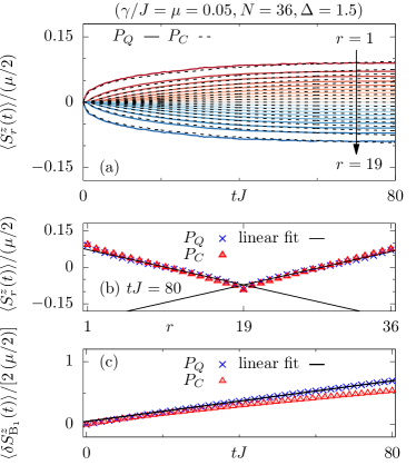
Because the prediction for the injected magnetization seems to be more sensitive to short-time deviations, as the ones visible in Fig. 3, we redo the analysis in Fig. 7 for (instead of ). In this way, the relevant time scale is increased. Simultaneously, we use another (instead of ). And indeed, as shown in Fig. 8 (c), the predictions for become closer to each other, which also leads to a slightly better agreement of the diffusion constants,
| (26) |
This observation indicates that one has to devote special attention to the role of and , to extract quantitative values for transport constants.
It is instructive to compare the values for the diffusion constants in Eq. (27) to other values in the literature. In the classical case, a value of has been found for the closed system [47], which agrees nicely with the value for the open system in Eq. (27). In the quantum case, the value is known with less precision and might be or larger in the closed system [21], while a value of has been found in the open system [23, 24], based on matrix-product-state simulations of the Lindblad equation, yet for a larger .
Finally, we demonstrate in Fig. 9 explicitly that our classical approach can be used for as many as lattice sites, where a quantum mechanical treatment is impossible, at least for the techniques used by us. While the required time to reach the steady state increases with , the additional computing time poses no conceptual problem. This result is particularly relevant, since it is obtained for a small , which is hard to treat on the basis of matrix product states. For the diffusion constant, we find
| (27) |
which is comparable to but larger than for , cf. Eq. (25), and indicates the importance of a finite-size analysis for the quantitative extraction of transport coefficients.
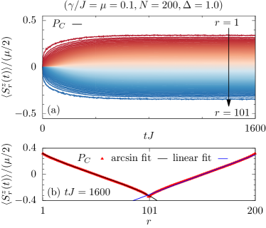
Since Fig. 9 focuses on , we depict in Fig. 10 additional data for . In comparison to , the steady-state profile for is not as well described by a linear function. Thus, we perform in Fig. 10 (b) a fit with another function,
| (28) |
which has been used in the quantum case before [24]. And indeed, also the classical case is well described by such a function, which indicates the usefulness of our classical approach for situations beyond the one of normal diffusion.
VI Conclusion
In summary, we have studied the Lindblad equation, as a central approach to the physics of open quantum systems. In this context, we have particularly focused on boundary-driven transport, where a steady state emerges in the long-time limit, which features a constant current and a characteristic density profile. The starting point of our study has been a recently suggested connection [72] between the dynamics in open and closed systems, which exits in certain cases. We have built on this connection for magnetization transport in the spin-1/2 XXZ chain with and without next-to-nearest-neighbor interactions, as integrability breaking perturbations. Specifically, we have shown that the time evolution of the open quantum system can be described by the use of classical correlation functions, as generated by the Hamiltonian equations of motion for classical real vectors. By comparing to exact numerical simulations of the Lindblad equation, we have demonstrated the accuracy of this description for a range of model parameters, but we have also pointed out its limitations by counterexamples. While this agreement is an interesting physical observation, it has also suggested that classical mechanics can be used to solve the Lindblad equation for comparatively large systems, which cannot be reached in a quantum mechanical treatment. Despite the approximate nature of this approach, one particular strength is the possibility to deal with small system-bath couplings, which are much harder to access on the basis of other numerical techniques. Furthermore, it seems to be possible that our approach can be applied to lattices in higher dimensions, as a promising direction of future research.
Acknowledgments
We thank Jochen Gemmer for fruitful discussions. This work has been funded by the Deutsche Forschungsgemeinschaft (DFG), under Grant No. 531128043, as well as under Grant No. 397107022, No. 397067869, and No. 397082825 within the DFG Research Unit FOR 2692, under Grant No. 355031190.
*
Appendix A Current in the steady state
In addition to the dynamics of the local magnetization, one can predict the current in the steady state. To this end, one needs the injected magnetization at the bath site , where the symbol is just a notation for the term “injected”. This injected magnetization can be predicted as [72]
| (29) |
with
| (30) |
which is slightly simpler than Eq. (15) in the main text and can be related to the current of interest. Since in the steady state all local currents are the same,
| (31) |
one only needs to know , which can be calculated as
| (32) |
Note that the factor occurring in the denominator is due to periodic boundary conditions, as magnetization can flow to the right and left of the bath contact.
The diffusion constant follows from via
| (33) |
for some site in the bulk of the system.
References
- Polkovnikov et al. [2011] A. Polkovnikov, K. Sengupta, A. Silva, and M. Vengalattore, Colloquium: Nonequilibrium dynamics of closed interacting quantum systems, Rev. Mod. Phys. 83, 863 (2011).
- Eisert et al. [2015] J. Eisert, M. Friesdorf, and C. Gogolin, Quantum many-body systems out of equilibrium, Nat. Phys. 11, 124 (2015).
- D’Alessio et al. [2016] L. D’Alessio, Y. Kafri, A. Polkovnikov, and M. Rigol, From quantum chaos and eigenstate thermalization to statistical mechanics and thermodynamics, Adv. Phys. 65, 239 (2016).
- Borgonovi et al. [2016] F. Borgonovi, F. Izrailev, L. Santos, and V. Zelevinsky, Quantum chaos and thermalization in isolated systems of interacting particles, Phys. Rep. 626, 1 (2016).
- Abanin et al. [2019] D. A. Abanin, E. Altman, I. Bloch, and M. Serbyn, Colloquium: Many-body localization, thermalization, and entanglement, Rev. Mod. Phys. 91, 021001 (2019).
- Bloch et al. [2008] I. Bloch, J. Dalibard, and W. Zwerger, Many-body physics with ultracold gases, Rev. Mod. Phys. 80, 885 (2008).
- Gemmer et al. [2004] J. Gemmer, M. Michel, and G. Mahler, Quantum thermodynamics, Lect. Notes Phys., Vol. 657 (Springer, Berlin, 2004).
- Goldstein et al. [2006] S. Goldstein, J. L. Lebowitz, R. Tumulka, and N. Zanghì, Canonical typicality, Phys. Rev. Lett. 96, 050403 (2006).
- Popescu et al. [2006] S. Popescu, A. J. Short, and A. Winter, Entanglement and the foundations of statistical mechanics, Nat. Phys. 2, 754 (2006).
- Reimann [2007] P. Reimann, Typicality for generalized microcanonical ensembles, Phys. Rev. Lett. 99, 160404 (2007).
- Bartsch and Gemmer [2009] C. Bartsch and J. Gemmer, Dynamical typicality of quantum expectation values, Phys. Rev. Lett. 102, 110403 (2009).
- Elsayed and Fine [2013] T. A. Elsayed and B. V. Fine, Regression relation for pure quantum states and its implications for efficient computing, Phys. Rev. Lett. 110, 070404 (2013).
- Steinigeweg et al. [2014] R. Steinigeweg, J. Gemmer, and W. Brenig, Spin-current autocorrelations from single pure-state propagation, Phys. Rev. Lett. 112, 120601 (2014).
- Heitmann et al. [2020] T. Heitmann, J. Richter, D. Schubert, and R. Steinigeweg, Selected applications of typicality to real-time dynamics of quantum many-body systems, Z. Naturforsch. A 75, 421 (2020).
- Jin et al. [2021] F. Jin, D. Willsch, M. Willsch, H. Lagemann, K. Michielsen, and H. De Raedt, Random state technology, J. Phys. Soc. Jpn. 90, 012001 (2021).
- Deutsch [1991] J. M. Deutsch, Quantum statistical mechanics in a closed system, Phys. Rev. A 43, 2046 (1991).
- Srednicki [1994] M. Srednicki, Chaos and quantum thermalization, Phys. Rev. E 50, 888 (1994).
- Rigol et al. [2008] M. Rigol, V. Dunjko, and M. Olshanii, Thermalization and its mechanism for generic isolated quantum systems, Nature 452, 854 (2008).
- Schollwöck [2005] U. Schollwöck, The density-matrix renormalization group, Rev. Mod. Phys. 77, 259 (2005).
- Schollwöck [2011] U. Schollwöck, The density-matrix renormalization group in the age of matrix product states, Ann. Phys. 326, 96 (2011).
- Bertini et al. [2021] B. Bertini, F. Heidrich-Meisner, C. Karrasch, T. Prosen, R. Steinigeweg, and M. Žnidarič, Finite-temperature transport in one-dimensional quantum lattice models, Rev. Mod. Phys. 93, 025003 (2021).
- Michel et al. [2003] M. Michel, M. Hartmann, J. Gemmer, and G. Mahler, Fourier’s Law confirmed for a class of small quantum systems, Eur. Phys. J. B 34, 325 (2003).
- Prosen and Žnidarič [2009] T. Prosen and M. Žnidarič, Matrix product simulations of non-equilibrium steady states of quantum spin chains, J. Stat. Mech. 2009, P02035 (2009).
- Žnidarič [2011] M. Žnidarič, Spin transport in a one-dimensional anisotropic Heisenberg model, Phys. Rev. Lett. 106, 220601 (2011).
- Breuer and Petruccione [2007] H.-P. Breuer and F. Petruccione, The theory of open quantum systems (Oxford University Press, 2007).
- Wichterich et al. [2007] H. Wichterich, M. J. Henrich, H.-P. Breuer, J. Gemmer, and M. Michel, Modeling heat transport through completely positive maps, Phys. Rev. E 76, 031115 (2007).
- De Raedt et al. [2017] H. De Raedt, F. Jin, M. I. Katsnelson, and K. Michielsen, Relaxation, thermalization, and Markovian dynamics of two spins coupled to a spin bath, Phys. Rev. E 96, 053306 (2017).
- Dalibard et al. [1992] J. Dalibard, Y. Castin, and K. Mølmer, Wave-function approach to dissipative processes in quantum optics, Phys. Rev. Lett. 68, 580 (1992).
- Michel et al. [2008] M. Michel, O. Hess, H. Wichterich, and J. Gemmer, Transport in open spin chains: A Monte Carlo wave-function approach, Phys. Rev. B 77, 104303 (2008).
- Zwolak and Vidal [2004] M. Zwolak and G. Vidal, Mixed-state dynamics in one-dimensional quantum lattice systems: A time-dependent superoperator renormalization algorithm, Phys. Rev. Lett. 93, 207205 (2004).
- Verstraete et al. [2008] F. Verstraete, V. Murg, and J. I. Cirac, Matrix product states, projected entangled pair states, and variational renormalization group methods for quantum spin systems, Adv. Phys. 57, 143 (2008).
- Weimer et al. [2021] H. Weimer, A. Kshetrimayum, and R. Orús, Simulation methods for open quantum many-body systems, Rev. Mod. Phys. 93, 015008 (2021).
- Kubo et al. [1991] R. Kubo, M. Toda, and N. Hashisume, Statistical physics II: Nonequilibrium statistical mechanics, Springer Series in Solid-State Sciences, Vol. 31 (Springer, Berlin, 1991).
- Windsor [1967] C. G. Windsor, Spin correlations in a classical Heisenberg paramagnet, Proc. Phys. Soc. 91, 353 (1967).
- Huber et al. [1969] D. L. Huber, J. S. Semura, and C. G. Windsor, Energy transport in magnetic chains, Phys. Rev. 186, 534 (1969).
- Lurie et al. [1974] N. A. Lurie, D. L. Huber, and M. Blume, Computer studies of spin and energy transport in one-dimensional Heisenberg magnets, Phys. Rev. B 9, 2171 (1974).
- De Raedt et al. [1981] H. De Raedt, J. Fivez, and B. De Raedt, Energy fluctuations in a classical Heisenberg chain, Phys. Rev. B 24, 1562 (1981).
- Müller [1988] G. Müller, Anomalous spin diffusion in classical Heisenberg magnets, Phys. Rev. Lett. 60, 2785 (1988).
- Gerling and Landau [1989] R. W. Gerling and D. P. Landau, Comment on “Anomalous spin diffusion in classical Heisenberg magnets”, Phys. Rev. Lett. 63, 812 (1989).
- Gerling and Landau [1990] R. W. Gerling and D. P. Landau, Time-dependent behavior of classical spin chains at infinite temperature, Phys. Rev. B 42, 8214 (1990).
- de Alcantara Bonfim and Reiter [1992] O. F. de Alcantara Bonfim and G. Reiter, Breakdown of hydrodynamics in the classical 1D Heisenberg model, Phys. Rev. Lett. 69, 367 (1992).
- Böhm et al. [1993] M. Böhm, R. W. Gerling, and H. Leschke, Comment on “Breakdown of hydrodynamics in the classical 1D Heisenberg model”, Phys. Rev. Lett. 70, 248 (1993).
- Srivastava et al. [1994] N. Srivastava, J.-M. Liu, V. S. Viswanath, and G. Müller, Spin diffusion in classical Heisenberg magnets with uniform, alternating, and random exchange, J. Appl. Phys. 75, 6751 (1994).
- Constantoudis and Theodorakopoulos [1997] V. Constantoudis and N. Theodorakopoulos, Nonlinear dynamics of classical Heisenberg chains, Phys. Rev. E 55, 7612 (1997).
- Oganesyan et al. [2009] V. Oganesyan, A. Pal, and D. A. Huse, Energy transport in disordered classical spin chains, Phys. Rev. B 80, 115104 (2009).
- Huber [2012] D. Huber, Spin diffusion in anisotropic Heisenberg chains: S 1/2, Physica B 407, 4274 (2012).
- Steinigeweg [2012] R. Steinigeweg, Spin transport in the XXZ model at high temperatures: Classical dynamics vs. quantum s=1/2 autocorrelations, EPL (Europhys. Lett.) 97, 67001 (2012).
- de Wijn et al. [2012] A. S. de Wijn, B. Hess, and B. V. Fine, Largest Lyapunov exponents for lattices of interacting classical spins, Phys. Rev. Lett. 109, 034101 (2012).
- Bagchi [2013] D. Bagchi, Spin diffusion in the one-dimensional classical Heisenberg model, Phys. Rev. B 87, 075133 (2013).
- Prosen and Žunkovič [2013] T. Prosen and B. Žunkovič, Macroscopic diffusive transport in a microscopically integrable Hamiltonian system, Phys. Rev. Lett. 111, 040602 (2013).
- Jin et al. [2013] F. Jin, T. Neuhaus, K. Michielsen, S. Miyashita, M. A. Novotny, M. I. Katsnelson, and H. D. Raedt, Equilibration and thermalization of classical systems, New J. Phys. 15, 033009 (2013).
- Jenčič and Prelovšek [2015] B. Jenčič and P. Prelovšek, Spin and thermal conductivity in a classical disordered spin chain, Phys. Rev. B 92, 134305 (2015).
- Das et al. [2018] A. Das, S. Chakrabarty, A. Dhar, A. Kundu, D. A. Huse, R. Moessner, S. S. Ray, and S. Bhattacharjee, Light-cone spreading of perturbations and the butterfly effect in a classical spin chain, Phys. Rev. Lett. 121, 024101 (2018).
- Das et al. [2019a] A. Das, K. Damle, A. Dhar, D. A. Huse, M. Kulkarni, C. B. Mendl, and H. Spohn, Nonlinear fluctuating hydrodynamics for the classical XXZ spin chain, J. Stat. Phys. 180, 238 (2019a).
- Das et al. [2019b] A. Das, M. Kulkarni, H. Spohn, and A. Dhar, Kardar-Parisi-Zhang scaling for an integrable lattice Landau-Lifshitz spin chain, Phys. Rev. E 100, 042116 (2019b).
- Li [2019] N. Li, Energy and spin diffusion in the one-dimensional classical Heisenberg spin chain at finite and infinite temperatures, Phys. Rev. E 100, 062104 (2019).
- Glorioso et al. [2021] P. Glorioso, L. V. Delacrétaz, X. Chen, R. M. Nandkishore, and A. Lucas, Hydrodynamics in lattice models with continuous non-Abelian symmetries, SciPost Phys. 10, 015 (2021).
- McRoberts et al. [2022] A. J. McRoberts, T. Bilitewski, M. Haque, and R. Moessner, Anomalous dynamics and equilibration in the classical Heisenberg chain, Phys. Rev. B 105, L100403 (2022).
- Roy et al. [2023] D. Roy, A. Dhar, H. Spohn, and M. Kulkarni, Robustness of Kardar-Parisi-Zhang scaling in a classical integrable spin chain with broken integrability, Phys. Rev. B 107, L100413 (2023).
- Benet et al. [2023] L. Benet, F. Borgonovi, F. M. Izrailev, and L. F. Santos, Quantum-classical correspondence of strongly chaotic many-body spin models, Phys. Rev. B 107, 155143 (2023).
- McRoberts et al. [2024] A. J. McRoberts, T. Bilitewski, M. Haque, and R. Moessner, Domain wall dynamics in classical spin chains: Free propagation, subdiffusive spreading, and soliton emission, Phys. Rev. Lett. 132, 057202 (2024).
- Elsayed and Fine [2015] T. A. Elsayed and B. V. Fine, Effectiveness of classical spin simulations for describing NMR relaxation of quantum spins, Phys. Rev. B 91, 094424 (2015).
- Gamayun et al. [2019] O. Gamayun, Y. Miao, and E. Ilievski, Domain-wall dynamics in the Landau-Lifshitz magnet and the classical-quantum correspondence for spin transport, Phys. Rev. B 99, 140301 (2019).
- Schubert et al. [2021] D. Schubert, J. Richter, F. Jin, K. Michielsen, H. De Raedt, and R. Steinigeweg, Quantum versus classical dynamics in spin models: Chains, ladders, and square lattices, Phys. Rev. B 104, 054415 (2021).
- Heitmann et al. [2022] T. Heitmann, J. Richter, F. Jin, K. Michielsen, H. De Raedt, and R. Steinigeweg, Spatiotemporal dynamics of classical and quantum density profiles in low-dimensional spin systems, Phys. Rev. Research 4, 043147 (2022).
- Park et al. [2024] P. Park, G. Sala, D. M. Pajerowski, A. F. May, J. A. Kolopus, D. Dahlbom, M. B. Stone, G. B. Halász, and A. D. Christianson, Quantum and classical spin dynamics across temperature scales in the S = 1/2 Heisenberg antiferromagnet, arXiv:2405.08897 (2024).
- Steinigeweg et al. [2009] R. Steinigeweg, M. Ogiewa, and J. Gemmer, Equivalence of transport coefficients in bath-induced and dynamical scenarios, EPL (Europhys. Lett.) 87, 10002 (2009).
- Žnidarič [2019] M. Žnidarič, Nonequilibrium steady-state Kubo formula: Equality of transport coefficients, Phys. Rev. B 99, 035143 (2019).
- Kundu et al. [2009] A. Kundu, A. Dhar, and O. Narayan, The Green–Kubo formula for heat conduction in open systems, J. Stat. Mech. 2009, L03001 (2009).
- Purkayastha et al. [2018] A. Purkayastha, S. Sanyal, A. Dhar, and M. Kulkarni, Anomalous transport in the Aubry-André-Harper model in isolated and open systems, Phys. Rev. B 97, 174206 (2018).
- Purkayastha [2019] A. Purkayastha, Classifying transport behavior via current fluctuations in open quantum systems, J. Stat. Mech. 2019, 043101 (2019).
- Heitmann et al. [2023] T. Heitmann, J. Richter, F. Jin, S. Nandy, Z. Lenarčič, J. Herbrych, K. Michielsen, H. De Raedt, J. Gemmer, and R. Steinigeweg, Spin- XXZ chain coupled to two Lindblad baths: Constructing nonequilibrium steady states from equilibrium correlation functions, Phys. Rev. B 108, L201119 (2023).
- Hogg et al. [2024] C. R. Hogg, J. Glatthard, F. Cerisola, and J. Anders, Stochastic simulation of dissipative quantum oscillators, arXiv:2406.05030 (2024).
- Kraft et al. [2024] M. Kraft, J. Richter, F. Jin, S. Nandy, J. Herbrych, K. Michielsen, H. De Raedt, J. Gemmer, and R. Steinigeweg, Lindblad dynamics from spatio-temporal correlation functions in nonintegrable spin- chains with different boundary conditions, Phys. Rev. Res. 6, 023251 (2024).
- Fendley [2016] P. Fendley, Strong zero modes and eigenstate phase transitions in the XYZ/interacting Majorana chain, J. Phys. A 49, 30LT01 (2016).
- Kemp et al. [2017] J. Kemp, N. Y. Yao, C. R. Laumann, and P. Fendley, Long coherence times for edge spins, J. Stat. Mech. 2017, 063105 (2017).
- Arnold [1978] V. I. Arnold, Mathematical Methods of Classical Mechanics, Graduate Texts in Mathematics (Springer, New York, 1978).
- Steinigeweg and Schmidt [2009] R. Steinigeweg and H.-J. Schmidt, Heisenberg-integrable spin systems, Math. Phys. Anal. Geom. 12, 19 (2009).