Multimer states in multilevel waveguide QED
Abstract
We study theoretically the interplay of spontaneous emission and interactions for the multiple-excited quasistationary eigenstates in a finite periodic array of multilevel atoms coupled to the waveguide. We develop an analytical approach to calculate such eigenstates based on the subradiant dimer basis. Our calculations reveal the peculiar multimerization effect driven by the anharmonicity of the atomic potential: while a general eigenstate is an entangled one, there exist eigenstates that are products of dimers, trimers, or tetramers, depending on the size of the system and the fill factor. At half-filling, these product states acquire a periodic structure with all-to-all connections inside each multimer and become the most subradiant ones.
The interplay of interactions and dissipation in the distributed nonlinear system can give rise to peculiar spatial patterns ranging from liquids [1, 2] to nonlinear optics [3, 4]. Periodic pattern formation has also been studied in quantum systems [5, 6, 7]. Nonlinear optimization for the states with minimal losses or maximal optical gain has also been recently proposed for analog computation, based on coupled laser networks [8] or coupled optical parametric oscillators [9].
Here, we explore the spatial structure of the multiple-excited states in the many-body quantum system, a finite periodic array of multilevel atoms, coupled to the waveguide, see Fig. 1. Such structures have now become available based on the superconducting qubits, optical atoms, and trapped cold atoms, and the corresponding field of waveguide quantum electrodynamics (waveguide QED) has emerged [10]. The system is inherently open because of the possibility of photon emission into the waveguide and features long-range photon-mediated couplings. The two-level atomic arrays are now relatively well studied both theoretically and experimentally. In particular, for the chiral two-level atom arrays, peculiar steady-state multipartite entangled patterns have been theoretically predicted in Ref. [11]. In non-chiral arrays, the transition from weak[12] to strong excitation regime has been studied in Ref. [13], and the formation of periodic dimerized eigenstates has been predicted. Double-excited subradiant states have recently been demonstrated in a 4-qubit array [14]. However, much less is known about a more general type of atoms with excited states, which correspond to actual superconducting transmon qubits [15]. Another relevant platform for the waveguide QED with multilevel atoms is a matter-wave QED platform [16, 17], where the role of photons is played by the unbound atomic states in the optical lattice [18].
Here, we show that the periodic pattern formation is a universal effect for multilevel atoms coupled to the waveguide: while most quasistationary eigenstates of the atomic array are spatially entangled, there also exist several peculiar multimerized product states:
| (1) |
Here, the indices label the atoms, the array size is a product of two integers, , and is the size of the multimer. The spectra of eigenstates with the same fill factor are split into different branches due to the anharmonicity of the atomic potential. Importantly, for fill factors , these multimer states are the most subradiant ones in their spectral branches. Examples of trimer () and tetramer () product states are illustrated by diagrams in Fig. 1(b,c), where each line between two sites and corresponds to a subradiant dimer excitation of the atoms and with opposite phases . One should multiply all such terms to obtain a multiple-excited subradiant eigenstate. We will show, that in the case of strong anharmonicity the number of lines per atom at half-filling condition is fixed to , which restricts the states to the products of multimers.
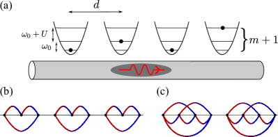
Theoretical model. We now proceed to the rigorous description of the multimerization. We consider a basic waveguide QED setup with multilevel atoms, periodically spaced near a waveguide and interacting via a waveguide mode. The system is schematically shown in Fig. 1 and can be described by the following effective Hamiltonian [19, 10]
| (2) |
We assume the Bose-Hubbard term is nonzero but much smaller than . In this case, the usual Markovian and rotating-wave approximations underlying the effective Hamiltonian Eq. (2) still hold. The raising operators obey the usual commutation relationship and , where is the number of levels per atom. The phase is , where is the distance between neighboring qubits and the parameter is the radiative decay rate of a single atom into the waveguide.
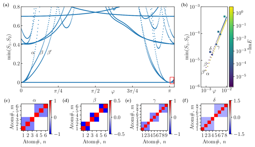
Multimer states. The two key parameters of our model are the relative anharmonicity strength and the phase , that controls the photon-mediated coupling between the atoms. For , the coupling is purely dissipative, and for it has an exchange character. Our goal is to analyze how the spatial profile of the multiple-excited eigenstates of Eq. (2) for larger anharmonicity depends on the coupling character. To this end, we calculate the entanglement entropy in the array of six 3-level atoms depending on . The array is divided into two subsystems and and the entanglement entropy is [20] , where is the reduced density matrix. We further define as the entanglement entropy with array containing the first three or two atoms, respectively. Figure 2 presents the minimal value for each state depending on . The overall picture has a period of [21]. The line at , corresponds to the trivial fully excited state of the array. Our main finding is the presence of the states where for and quadratically increases as is detuned from [see also zoomed in Fig. 2(b)]. In order to understand these states we plot in Fig. 2(c–d) their corresponding correlation functions We find that the state labelled as is the dimerized state [13],
| (3) |
at and state is just the particle-hole inversion of state . One can replace the ground state with the full excited state and all the creation operators with the annihilation operators in Eq. (3) to obtain the expression of state . The state is a trimer state, at it is given by
| (4) |
in agreement with the general ansatz Eq. (1). Inspired by this finding, we also numerically calculate the entanglement entropy of the most subradiant states at half-filling for , and , . This yields two more states with at , see Fig. 2(b). Their correlations are plotted in Fig. 2(e) and Fig. 2(f). Here, the entanglement entropy of the states and is calculated for subsystem containing the first three and four atoms, respectively. Hence, the state is a direct product of three trimers, as illustrated in Fig. 1(b), and state is a direct product of two tetramers [see Fig. 1(c)]. We will further term them a trimer state and a tetramer state.
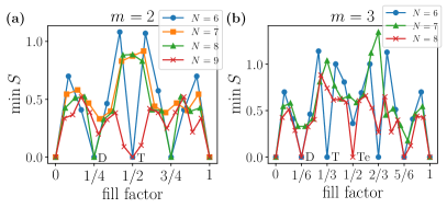
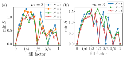
The presence of the multimer states with zero entanglement entropy, found in Fig. 2, turns out to be a general mesoscopic property of the finite system that is manifested for properly matching the number of atoms , the number of excited levels per atom and the fill factor . Here we define the fill factor for each eigenstates as . where is the number of excitations. This is possible because the Hamiltonian Eq. (2) commutes with the excitation number operator .
Figure 3 summarizes our calculations of entanglement entropy for with [Fig. 3(a)] and with [Fig. 3(b)]. For every eigenstate we calculated the entropy for all possible divisions of the array into two parts with at least two atoms in each part. Next, for each value of the fill factor we present the minimum value of . The calculation in Fig. 3 shows sharp minima corresponding to the specific values of when the number of fits an integer multiple of dimers, trimers or tetramers. In particular, when , the dimer state and trimer state are allowed. For multiples of 3 and 2 like , there is a dimer state at , the particle-hole inversion of that dimer state at and a trimer state at . For being just a multiple of 3 like , there is only a trimer state at half-filling. For being just a multiple of 2 like , there is only a dimer state at and its inversion. For neither dimer nor trimer states are possible. We note that the dimer states at here can be considered as inherited from the array with two levels per atom at half-filling.
When , tetramer states are allowed. Next, for the multiples of 4 like , there is a tetramer state at half-filling. Besides, for multiples of 2 like , there are dimer states at and their inversion at . For multiples of 3 like , there is a trimer state at and its inversion at . For a prime number of no multimer states are possible.
As shown in Fig. 2(b) and Fig. 3, the multimer states at are subradiant. We now present a perturbative approach to study the subradiant states in short-period arrays when is close to 0. Taylor expansion of the atom-photon interaction part of the Hamiltonian Eq. (2) results in
| (5) |
where
| (6) |
We are looking for subradiant states, where the expectation value of is zero and the imaginary part of complex energies is proportional to . In the Supplementary Materials we prove that such states must be fully composed of dimer operators of the type , see e.g. Eqs. (3),(4). This is a generalization of the single-excited dark dimer state in two atoms where the destructive interference suppresses photon emission [22]. For a given set of numbers , we can fully capture all the subradiant states by such a dimer basis. Importantly, this dimer basis is not orthogonal, but it is still complete. The completeness of the basis also proves the half-filling theorem for subradiant states: the subradiant states only exist for . This straightforwardly follows from the fact that the dimer basis can not be constructed for and generalizes the results in Ref. [13] for the two-level atom case.
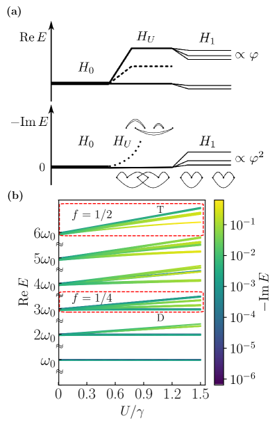
Now we describe the degenerate perturbation theory in and to construct subradiant states, illustrated in Fig. 4(a). Both and lead to the splitting of the real part of the energy spectrum. The anharmonic term also induces a nonzero decay rate for those states that are not eigenstates of . These states would get mixed up with other non-subradiant states as the dashed line in Fig. 4(a).
After the splitting by the anharmonicity potential, the remaining states are shaped by the degenerate perturbation in . Their imaginary parts of energies are contributed by the first-order perturbation in and the second-order perturbation in . The real parts are contributed by the expectation value of , which is an integer multiple of , and the first order perturbation of .
Figure 4(b) illustrates this perturbation process by tracking the energy dependence of subradiant states on in a six-atom array with three levels per atom. When the number of excitations is , the states do not feel the effect of anharmonicity and remain subradiant. When , the subradiant states are split into three branches with different real parts of energies, . The slopes can be analytically calculated when performing the degenerate perturbation. Only the states in the lowest branch are eigenstates of and stay subradiant. We define such a branch as a subradiant branch. On the other hand, the states in the upper two branches are not eigenstates of and thus become bright as is turned on. Following the same procedure, when , there are four branches with . Only the lowest and highest branches with integer slopes are subradiant. When , there are five branches with . One of the branches with is subradiant while the other one is not. When , there are five branches, , and none of them are subradiant. When , there are three: , the highest branch are subradiant.
Among all the subradiant states above, we find that the dimer state at is the most subradiant state in the branch , and the trimer state at is the most subradiant state in the branch as labeled in Fig. 4(b). The intuitive explanation is that these multimer states, by construction, minimize the distances between the excitations and, as a result, minimize the expectation values of the Hamiltonians and in Eq. ( Multimer states in multilevel waveguide QED) providing the radiative decay. We note that the half-filling requirement for an -level atom means that each atom in the diagram of type Fig. 1(b,c) is connected to exactly neighbors.
In order to further illustrate the formation of the trimer state in Fig. 4(b), we introduce the concept of trimer basis. The difference between the full trimer basis and the particular trimer state in Eq. (4) is that the index 1,2,3 in Eq. (4) can be any other number set. Trimer basis states, as a subset of dimer basis, are eigenstates of . They remain subradiant while other states, like those involving products with more than one dimer operator , get mixed up, as shown in Fig. 4(a). After degenerate perturbation of , the trimer state Eq. (4) wins as the most subradiant because of its minimum expectation values of among all the five trimer basis states. Generally, at half-filling, only multimer basis states would stay subradiant after the degenerate perturbation of . There is at most one subradiant branch. Therefore, if a multimer state exists at half-filling, it is the most subradiant state.
For comparison, we also consider in the Supplementary Materials another model of multilevel atoms that have equidistant levels. In this model, there is no anharmonic term; hence, there is no multimer state for . Instead, approximate higher-order dimer states of type become possible. Based on the intuitions above, such states with nearest-neighbor dimer couplings could be expected to be the most subradiant states at half-filling. However, we show in Supplementary Materials that such an expectation doesn’t always hold.
Summary. Our findings provide a simple recipe for constructing multiple-excited subradiant states in multilevel atomic arrays. We show how the destructive interference and anharmonic level structure favor the multimer product states. We have tested this recipe in a one-dimensional array of multilevel atoms coupled to a waveguide. It is still an open question whether this intuition applies to two- or three-dimensional setups, which are now also emerging [23] or to the waveguides with a more complex photon dispersion law [24].
References
- Manneville [2006] P. Manneville, Rayleigh-Bénard convection: Thirty years of experimental, theoretical, and modeling work, in Dynamics of Spatio-Temporal Cellular Structures: Henri Bénard Centenary Review, edited by I. Mutabazi, J. E. Wesfreid, and E. Guyon (Springer New York, New York, NY, 2006) pp. 41–65.
- Cassani et al. [2021] A. Cassani, A. Monteverde, and M. Piumetti, Belousov-Zhabotinsky type reactions: the non-linear behavior of chemical systems, J. Math. Chem. 59, 792 (2021).
- Arecchi [1995] F. Arecchi, Optical morphogenesis: pattern formation and competition in nonlinear optics, Physica D 86, 297 (1995).
- Zhang et al. [2015] L. Zhang, W. Xie, J. Wang, A. Poddubny, J. Lu, Y. Wang, J. Gu, W. Liu, D. Xu, X. Shen, Y. G. Rubo, B. L. Altshuler, A. V. Kavokin, and Z. Chen, Weak lasing in one-dimensional polariton superlattices, Proc. Nat. Acad. Sci. 112, E1516 (2015).
- Léonard et al. [2017] J. Léonard, A. Morales, P. Zupancic, T. Esslinger, and T. Donner, Supersolid formation in a quantum gas breaking a continuous translational symmetry, Nature 543, 87–90 (2017).
- Li et al. [2017] J.-R. Li, J. Lee, W. Huang, S. Burchesky, B. Shteynas, F. u. Top, A. O. Jamison, and W. Ketterle, A stripe phase with supersolid properties in spin–orbit-coupled Bose–Einstein condensates, Nature 543, 91–94 (2017).
- Hertkorn et al. [2021] J. Hertkorn, J.-N. Schmidt, M. Guo, F. Böttcher, K. S. H. Ng, S. D. Graham, P. Uerlings, T. Langen, M. Zwierlein, and T. Pfau, Pattern formation in quantum ferrofluids: From supersolids to superglasses, Phys. Rev. Res. 3, 033125 (2021).
- Tradonsky et al. [2019] C. Tradonsky, I. Gershenzon, V. Pal, R. Chriki, A. A. Friesem, O. Raz, and N. Davidson, Rapid laser solver for the phase retrieval problem, Science Advances 5, eaax4530 (2019).
- McMahon et al. [2016] P. L. McMahon, A. Marandi, Y. Haribara, R. Hamerly, C. Langrock, S. Tamate, T. Inagaki, H. Takesue, S. Utsunomiya, K. Aihara, R. L. Byer, M. M. Fejer, H. Mabuchi, and Y. Yamamoto, A fully programmable 100-spin coherent Ising machine with all-to-all connections, Science 354, 614 (2016).
- Sheremet et al. [2023] A. S. Sheremet, M. I. Petrov, I. V. Iorsh, A. V. Poshakinskiy, and A. N. Poddubny, Waveguide quantum electrodynamics: Collective radiance and photon-photon correlations, Rev. Mod. Phys. 95, 015002 (2023).
- Pichler et al. [2015] H. Pichler, T. Ramos, A. J. Daley, and P. Zoller, Quantum optics of chiral spin networks, Phys. Rev. A 91, 042116 (2015).
- Zhang and Mølmer [2019] Y.-X. Zhang and K. Mølmer, Theory of subradiant states of a one-dimensional two-level atom chain, Phys. Rev. Lett. 122, 203605 (2019).
- Poshakinskiy and Poddubny [2021] A. V. Poshakinskiy and A. N. Poddubny, Dimerization of many-body subradiant states in waveguide quantum electrodynamics, Phys. Rev. Lett. 127, 173601 (2021).
- Zanner et al. [2022] M. Zanner, T. Orell, C. M. F. Schneider, R. Albert, S. Oleschko, M. L. Juan, M. Silveri, and G. Kirchmair, Coherent control of a multi-qubit dark state in waveguide quantum electrodynamics, Nat. Phys. 18, 538 (2022).
- Krantz et al. [2019] P. Krantz, M. Kjaergaard, F. Yan, T. P. Orlando, S. Gustavsson, and W. D. Oliver, A quantum engineer’s guide to superconducting qubits, Appl. Phys. Rev. 6, 021318 (2019).
- de Vega et al. [2008] I. de Vega, D. Porras, and J. I. Cirac, Matter-wave emission in optical lattices: Single particle and collective effects, Phys. Rev. Lett. 101, 260404 (2008).
- Kwon et al. [2022] J. Kwon, Y. Kim, A. Lanuza, and D. Schneble, Formation of matter-wave polaritons in an optical lattice, Nature Physics 18, 657 (2022).
- Kim et al. [2023] Y. Kim, A. Lanuza, and D. Schneble, Super- and subradiant dynamics of quantum emitters mediated by atomic matter waves (2023), arXiv:2311.09474 [quant-ph] .
- Caneva et al. [2015] T. Caneva, M. T. Manzoni, T. Shi, J. S. Douglas, J. I. Cirac, and D. E. Chang, Quantum dynamics of propagating photons with strong interactions: a generalized input–output formalism, New J. Phys. 17, 113001 (2015).
- Eisert et al. [2010] J. Eisert, M. Cramer, and M. B. Plenio, Colloquium: area laws for the entanglement entropy, Rev. Mod. Phys. 82, 277 (2010).
- Ivchenko et al. [1994] E. L. Ivchenko, A. I. Nesvizhskii, and S. Jorda, Bragg reflection of light from quantum-well structures, Phys. Solid State 36, 1156 (1994).
- DeVoe and Brewer [1996] R. G. DeVoe and R. G. Brewer, Observation of superradiant and subradiant spontaneous emission of two trapped ions, Phys. Rev. Lett. 76, 2049 (1996).
- Tečer et al. [2024] M. Tečer, M. Di Liberto, P. Silvi, S. Montangero, F. Romanato, and G. Calajó, Strongly interacting photons in 2D waveguide QED, Phys. Rev. Lett. 132, 163602 (2024).
- Zhang et al. [2023] X. Zhang, E. Kim, D. K. Mark, S. Choi, and O. Painter, A superconducting quantum simulator based on a photonic-bandgap metamaterial, Science 379, 278 (2023).
Supplementary materials
S0.1 Subradiant dimer basis
Here, we prove that subradiant states must be fully composed of dimer operators of the type at . First of all, we want to construct a mapping between the quantum raising operators and polynomials.
Any eigenstate with excitations can always be written as
| (S1) |
where the tensor turns to zero if any of the indices coincide due to the limit of levels. Here, we define a mapping from the states to the homogeneous polynomials by turning the creation operators into and the tensor into coefficients.
| (S2) |
We also notice that the annihilation operator on a state can be mapped to a derivative to the polynomial .
We are looking for the eigenstates of the Hamiltonian in Eq. ( Multimer states in multilevel waveguide QED) with zero eigenvalues
| (S3) |
We note that can be written as
| (S4) |
Therefore, a state should fulfill the condition
| (S5) |
so that . This equation is equivalent to the following condition for the polynomials
| (S6) |
Mathematically, it means that is a Lagrange polynomial, which can be written as . According to the mapping we defined, the subradiant states should be fully composed of dimer operators.
S0.2 Counting subradiant states when .
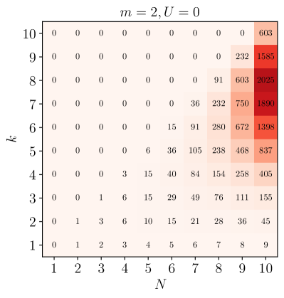
When there is no anharmonic term , the number of subradiant states is equal to the number of linear independent dimer basis states. These states can be counted with straightforward but rather tedious combinatorics. Here, we present a rigorous formula to obtain the number of subradiant states with any given number of , , and as . Even when the anharmonic term exists, the formula provides the number of dimer basis states that will be useful for perturbation calculation.
First, we replace the operators in the previous section with for . A dimer basis can be mapped to a homogeneous polynomial . So the number of linear independent dimer basis is equal to the number of all possible terms with a constraint and . The number of excitations is thus the order of polynomial. We remind that the number of levels per atom is .
Without the second constraint, the number of all possible terms is just the binomial coefficient that counts the number of ways to put identical balls into different boxes.
Now we take into account the constraint . When , this constraint is automatically satisfied. Therefore the number of subradiant states is just . However, when , we should subtract the number of terms that do not satisfy this constraint. There are two possible variants depending on the index of . When , the constraint means that the terms like should obey . Here, the “bad” terms to be discarded can be constructed as putting balls into one box and distributing the rest into all the boxes. So, the number of discarded terms is When , the constraint means that we must make sure the degree of is no larger than . We note, that satisfies . Thus, we only need to set the coefficient of terms whose order of is to be zero, and the terms with higher degrees of would be then zero automatically. As such, we count the number of terms with constraint that is equal to
| (S7) |
As a result, when , the number of subradiant states is
The case when is even more complicated. The constraint on , by the analogy of putting balls into boxes, demands that there should be no more than balls in boxes. There exist two kinds of bad terms that we have to exclude. (i) There are at least balls in one box, or at least balls in two boxes. The number of balls in the rest boxes must be no more than . The number of such bad terms is
| (S8) |
(ii) There are at least balls in one box. The remaining balls are then placed to make sure that the number of balls newly added into each box does not exceed . The number of such bad terms is
| (S9) |
Here the term comes from the constraint on in Eq. (S7).
The constraint on introduces other types of terms with a constraint and , since in Eq. (S8) and Eq. (S9) we have already excluded the terms with the degrees of larger than :
| (S10) |
With the calculation above, when , the number of subradiant states is
| (S11) |
When , following the similar procedure, we obtain the formula
| (S12) |
One can further obtain the number of subradiant states for larger . When , the formulas above reduce to
| (S13) |
which is the result in Ref. [13].
There is another approach to calculate the number of subradiant states. The number of subradiant states at excitation is the difference of the number of eigenstates at and the number of eigenstates at . While the number of eigenstates at is equal to the number of terms with constraint and . The idea is straightforward. The number of eigenstates at is the number of decay channels for eigenstates at , as illustrated in Fig. S1. If the number of decay channels is smaller than the number of eigenstates, some eigenstates do not decay and they are subradiant.
For example, at , there are
| (S14) |
totally terms. At , there are
| (S15) |
totally terms. So the number of subradiant states at is .

We have checked that both approaches give the same result for the number of subradiant states as the numerical simulation in Fig. S2.
S0.3 Energies of subradiant states
Here, we present the details of the perturbation theory in and for subradiant states. The energies of subradiant states at lowest order of are
| (S16) |
The value of is given by the first order perturbation in ,
| (S17) |
and the value is given by the first order perturbation in :
| (S18) |
The factor of here stems from Eq. (5) in the main text, that is .
The imaginary part is given by the second order perturbation in . It involves all the other non-subradiant states at the same excitation number since we assume that ,
| (S19) |
For , this expression reduces to
| (S20) |
Since we do not have an explicit equation to analytically calculate all the eigenstates of , the value can only be obtained numerically. In numerical calculation of the eigenstates of , it is convenient to introduce small perturbation to split the degeneracy.
S0.4 Multilevel atoms with equidistant levels.
In the main text we focus on the atoms described by a Bose-Hubbard-type model, where the anharmonic term splits the states into different branches as shown in Fig. 4. Here, we consider an atomic array with a finite number of equidistant levels per atom.
Figure S3 shows the fill-factor dependence of the minimum value of entanglement entropy for the equidistant level model. Comparing with Fig. 3 in the main text, we find that when , we find no multimer state below half-filling. At half-filling, in addition to the trimer states at in Fig. S3(a), there appears an approximate higher-order dimer state at with nearly zero entanglement entropy:
| (S21) |
In Fig. S3(b), at half-filling, we find another approximate higher-order dimer state at instead of the tetramer state.
| (S22) |
At , higher-order dimer states are also possible.
The fact that no multimer state survives below half-filling emphasizes the importance of the anharmonic term . Without the degenerate perturbation of in Fig. 4, these multimer states would get mixed up by the degenerate perturbation of .
It is not clear yet why the multimer states still exist above half-filling, but this effect is out of the scope of the current study.
| 2 | 3 | 4 | 5 | 6 | 7 | 8 | 9 | 10 | |
|---|---|---|---|---|---|---|---|---|---|
| 0.38888 | 1.82 | 5.6977 | 15.5693 | 41.10887 | 110.144 | 306.0854 | 887.6915 | 2679.763 | |
| 1 | 3 | 5.5 | 8.125 | 10.6875 | 13.125 | 15.4375 | 17.6484375 | 19.78515625 | |
| 6.304762 | 15.9961 | 34.78263 | 71.52311 | 147.5097 | 317.7914 | 733.2622 | 1827.4642 | 4894.2766 | |
| 0.06168 | 0.03793 | 0.2978 | 0.02679 | 0.02608 | 0.02641 | 0.02704 | 0.02752 | 0.02767 |
In the absence of , as shown in Fig. S3, there are higher-order dimer states at half-filling. We will now discuss when such states are exact eigenstates and when they are the most subradiant ones. The general expression of higher-order dimer states is
| (S23) |
In a two-level atomic system, , the dimer state is an eigenstate of with eigenvalue . So it’s exact. However, when , is not an eigenstate of ,
| (S24) |
When , the expression for the exact term is . We remind that . We find that is perpendicular to any dimer basis because of the symmetry: after swapping and , and , is still but becomes . So for , higher-order dimer states are still exact eigenstates.
When , gets mixed up with the other states. However, the degree of mixing is small. The qualitative reason is that even though is not an exact eigenstate of , it still has the lowest possible expectation value of among all the dimer basis states. This is because this state involves only the dimers with adjacent sites. As a result, when solving the degenerate perturbation equation , one would get an eigenvector close to with the eigenvalue close to . After the perturbation, one would get the eigenstate .
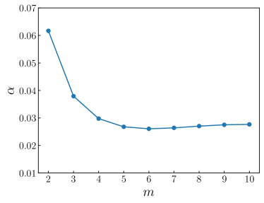
We will now demonstrate that the higher-order dimer state is the most subradiant one only for small values of and . By construction, has also the minimum expectation value of . Then according to Eq. (S19), the value . This makes a good candidate for the most subradiant state. However, another contribution to the imaginary part of the energy, grows exponentially with . As a result, it turns out that for large of , the state becomes surpassed by other subtadiant states. To demonstrate this, we take the case as an example. After normalization of Eq. (S23) with , we find that .
Since is orthogonal to non-subradiant states, we take an approximation of Eq. (S20),
| (S25) |
Our numerical finding is that . And for and the state becomes the second most subradiant state. For , when , is not the most subradiant. For , the maximum value of that we were able to consider numerically on a workstation with 150 Gb of RAM was 10. We have verified that the state stays the most subradiant until this value of .
S0.5 Shadows of the multimer states
In the main text, we demonstrate the existence of the multimer states that are direct products of dimers, trimers, tetramers, etc. In the previous section (dimer basis) we show that the physical reasons behind the multimerization effect is highly relevant with subradiance. This intuition can be supported by some states that look like shadows of the multimer states. These states appear when the number of atoms is not an integer multiple of ,, etc., and does not meet the requirements for multimerization. They are not direct product states but are related to the multimer states.
For example, in a 5-atom array with 3 levels per atom, when , the most subradiant state with 4 excitations is
| (S26) |
One can neglect the last two terms and approximate this state as
| (S27) |
While such states are not direct product state and their entanglement entropy is nonzero, they further demonstrate the tendency of the system to form multimer states.