[a]T. San José
The distribution amplitude of the -meson
Abstract
In this proceeding we determine the distribution amplitude of the -meson from first principles. This quantity appears as a consequence of factorization theorems, and it is necessary to compute the amplitude of multiple exclusive processes. Since it is defined along a light-cone, its calculation via lattice QCD was impossible until recently, when a generalization to Euclidean metric was proposed, and a connection to the physical limit was established. We briefly explain the method of short distance factorization, which allows us to compute the distribution amplitude, and our lattice setup. After summarizing the steps for the continuum and chiral extrapolation, we present our results and compare them to two alternative determinations, one using non-relativistic QCD and another solving the Dyson-Schwinger equations; we find a large discrepancy with the former.
1 Introduction
Factorization theorems are a fundamental tool to study the internal structure of hadrons. They separate the amplitude of many scattering processes into two pieces: The interaction between the scattering probe and the target’s quarks and gluons, which is calculable in perturbation theory; and the internal structure of the various hadrons, which requires non-perturbative methods. In particular, distribution amplitudes of heavy mesons describe the momentum distribution of the quarks along the longitudinal axis, and they are necessary to compute the amplitude of decays, deeply virtual meson production, and other exclusive processes (see [1] for a review). For a pseudoscalar charmonium state like , its distribution amplitude (DA)is defined by a bi-local matrix element [1],
| (1) |
where the Wilson line assures gauge invariance, the meson moves along the axis , the quark’s momentum fraction in the longitudinal direction is , and the quarks are separated along the direction . Given its non-perturbative nature, the idea of computing this quantity ab initio using lattice QCD arises. However, the condition prohibits the direct calculation of equation 1 in Euclidean space. This was until 2013, when Ji introduced a generalization to space-like separations [2] known as quasi-distributions, where one could use and in Euclidean space. The new function tends towards the light-cone DA (LCDA)when taking the limit appropriately. However, as it was pointed out in [3], lattice simulations must include data at to take the infinite limit safely, a condition our ensembles cannot fulfill without introducing sizeable lattice artifacts. Instead, in our project we consider the equivalent approach outlined in [3], known as pseudo-distributions, which converge to the physical quantity in the limit . The factor plays an analogous role to a renormalization parameter .
In the remainder of this proceeding, we summarize how to extract the pseudo-DAfrom the lattice, take the continuum limit, and match to the LCDA. Besides, we compare our results with those from Dyson-Schwinger (DS)[4] and non-relativistic QCD (NRQCD)[5] determinations. For a complete report on this work, we direct the avid reader to [6].
2 Methodology
The first step in Euclidean space is to compute the matrix element [7]
| (2) |
where and is the Ioffe time. We consider the asymmetric configuration to make use of all lattice sites, and we recover the symmetric structure of equation 1 using translation invariance. Next, we can separate some higher-twist contamination using the Lorentz decomposition [7]
| (3) |
where carries the leading twist as well as some high twist component proportional to , and is a purely higher-twist effect. To isolate , we select the component , such that . The matrix element is multiplicatively renormalizable at all orders in perturbation theory [8], and the normalization constant is a function of alone. Then, we form a ratio that retains the physical evolution of the LCDAwhile reducing the contamination from the lattice artifacts and higher twist [7, 9, 10],
| (4) |
Equation 4 is the reduced Ioffe-time pseudo-DA, which does not require any additional renormalization, and so it has a well defined continuum limit. This is the actual quantity we extract from the lattice data. Equation 4 is related to the DAon the light-cone via a matching kernel derived in [11, 12] at NLOin perturbation theory,
| (5) |
where we choose the renormalization scheme at a scale . Equation 5 is an inverse problem, because we attempt to reconstruct the right-hand sidewith only a limited data set. To solve it, we model the LCDAtaking inspiration from its conformal expansion [1],
| (6) |
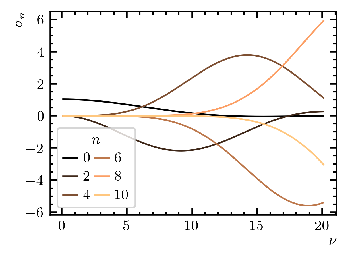
The coefficients and are fitted with the lattice data, is a beta function, and are shifted Gegenbauer polynomials, defined in the domain . The assymptotic value, is recovered from equation 6 setting . A similar approach for parton distribution functions (PDFs)can be seen in [13]. Then, we can replace equation 6 in equation 5 and compute the integrals using properties of the Gegenbauer polynomials, such that
| (7) |
The new set of functions are plotted in figure 1 for representative values of our simulations, and their full expressions are reported in [6].
3 Lattice calculation
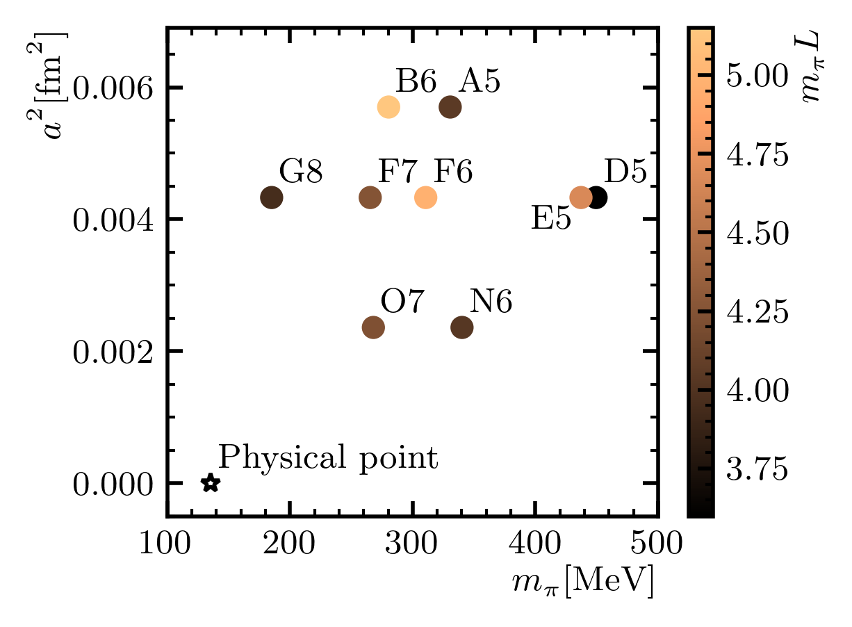
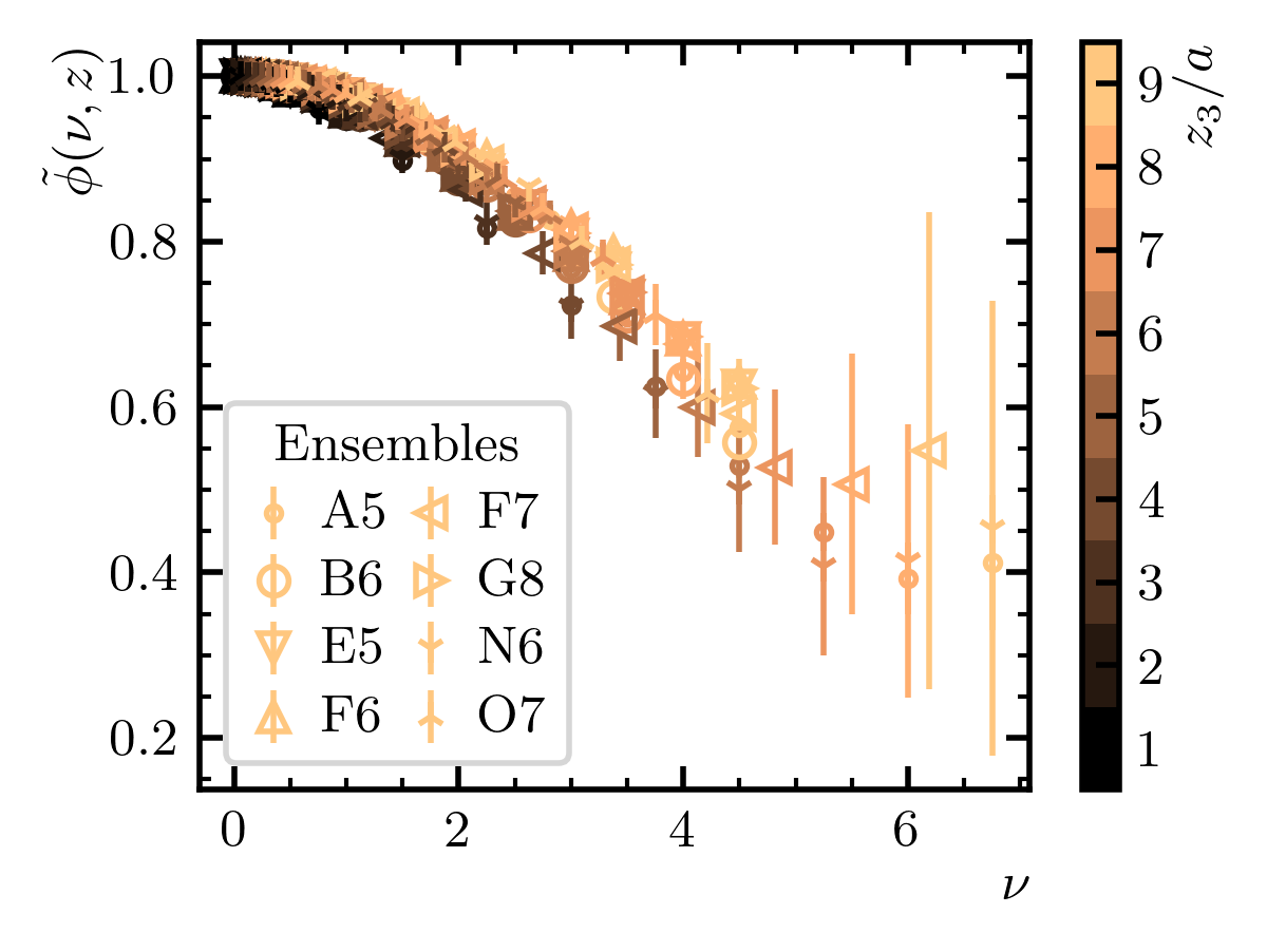
We employ the CLSensembles collected in figure 1. For details on the gauge simulations and the scale setting, see [14]. We employ quark all-to-all propagators with wall sources diluted in spin, and we solve the Dirac equation with deflated SAP-GCR, and the contractions are performed with a costum version of the domain decomposition HMC (DD-HMC)algorithm. The momentum is set employing partially twisted boundary conditions, and to create a realistic meson interpolator we solve a 4x4 generalized eigenvalue problemwith four levels of Gaussian smearing. Out of the two Wick contractions, we only compute the quark-connected diagram, as we expect the disconnected contribution to have a strong OZIsuppression. Upon averaging over the spatial lattice points, the double ratio in equation 4 shows a mild time dependence, and we select picking a particular time slice from a plateau range. Selecting the same time slice for all on a given ensemble, we can keep correlations intact throughout our analysis, and varying the selected time slice we explore the systematic uncertainty [6]. Figure 2 shows equation 4 on all our ensembles. We observe that all data points, which we denote by , fall in a nearly universal line, but several corrections remain to be applied if one is to extract equation 1: First, we need to model the quark-mass dependence to give a prediction at the physical value; second, we need to take the continuum limit removing the lattice artifacts; third, we have to model the remaining higher-twist contamination.
We combine these steps in a single fit, where we minimize a employing a custom implementation of the variable projectionalgorithm, and we fit our data to the model [6]
| (8) | ||||
which gathers all the aforementioned requirements. See [13] for a study of PDFsusing a similar approach. We use [15] to render all terms dimensionless. The auxiliary functions , , , etc., have a similar behavior in to that of , and they are defined in very similar fashion to equation 6. Since , our fit function is only sensitive to the first coefficient in equation 6, and we limit ourselves to determine the value of . At the minimum , we obtain , where the uncertainty includes both statistics and systematics. This is our main result, and we stress that knowing the first coefficient in equation 6 is sufficient to describe the DAin our range of Ioffe times based on the good fit quality. The DAis analytic in Ioffe-time space, and therefore we Fourier-transform equation 6 to compare it to two other determinations using NRQCD[5] and DSequations [4]. The various results are gathered in figure 3, and we observe good agreement between our result and [4], but there are large discrepancies with the non-relativistic calculation.

4 Conclusions and Outlook
We present the first lattice calculation of the -meson DA. We give the DAin closed form using equation 6 truncating and using . This parameterization is sufficient to fit the lattice data, which is generated following the pseudo-distribution approach. Our results are obtained in the continuum limit at the physical quark masses (with exact isospin symmetry) and at leading twist. Our determination is in strong tension with results from NRQCD. In the future, we plan to expand our analysis to other heavy states as well as to upgrade our simulations to flavors in the sea.
Acknowledgments
The work by J.M. Morgado Chávez has been supported by P2IO LabEx (ANR-10-LABX-0038) in the framework of Investissements d’Avenir (ANR-11-IDEX-0003-01). The work by T. San José is supported by Agence Nationale de la Recherche under the contract ANR-17-CE31-0019. This project was granted access to the HPC resources of TGCC (2021-A0100502271, 2022-A0120502271 and 2023-A0140502271) by GENCI. The authors thank Michael Fucilla, Cédric Mezrag, Lech Szymanowski, and Samuel Wallon for valuable discussions.
References
- [1] M. Diehl, Generalized parton distributions, Phys. Rept. 388 (2003) 41 [hep-ph/0307382].
- [2] X. Ji, Parton Physics on a Euclidean Lattice, Phys. Rev. Lett. 110 (2013) 262002 [1305.1539].
- [3] A.V. Radyushkin, Quasi-parton distribution functions, momentum distributions, and pseudo-parton distribution functions, Phys. Rev. D 96 (2017) 034025 [1705.01488].
- [4] M. Ding, F. Gao, L. Chang, Y.-X. Liu and C.D. Roberts, Leading-twist parton distribution amplitudes of S-wave heavy-quarkonia, Phys. Lett. B 753 (2016) 330 [1511.04943].
- [5] Chung, Ee, Kang, Kim, Lee and Wang, Pseudoscalar Quarkonium+gamma Production at NLL+NLO accuracy, JHEP 10 (2019) 162 [1906.03275].
- [6] B. Blossier, M. Mangin-Brinet, J.M. Morgado Chávez and T. San José, The distribution amplitude of the -meson at leading twist from Lattice QCD, 2406.04668.
- [7] A. Radyushkin, Nonperturbative Evolution of Parton Quasi-Distributions, Phys. Lett. B 767 (2017) 314 [1612.05170].
- [8] T. Ishikawa, Y.-Q. Ma, J.-W. Qiu and S. Yoshida, Renormalizability of quasiparton distribution functions, Phys. Rev. D 96 (2017) 094019 [1707.03107].
- [9] K. Orginos, A. Radyushkin, J. Karpie and S. Zafeiropoulos, Lattice QCD exploration of parton pseudo-distribution functions, Phys. Rev. D 96 (2017) 094503 [1706.05373].
- [10] J. Karpie, K. Orginos and S. Zafeiropoulos, Moments of Ioffe time parton distribution functions from non-local matrix elements, JHEP 11 (2018) 178 [1807.10933].
- [11] A.V. Radyushkin, Quark pseudodistributions at short distances, Phys. Lett. B 781 (2018) 433 [1710.08813].
- [12] A.V. Radyushkin, Generalized parton distributions and pseudodistributions, Phys. Rev. D 100 (2019) 116011 [1909.08474].
- [13] HadStruc collaboration, The continuum and leading twist limits of parton distribution functions in lattice QCD, JHEP 11 (2021) 024 [2105.13313].
- [14] P. Fritzsch, F. Knechtli, B. Leder, M. Marinkovic, S. Schaefer, R. Sommer et al., The strange quark mass and Lambda parameter of two flavor QCD, Nucl. Phys. B 865 (2012) 397 [1205.5380].
- [15] FLAG collaboration, FLAG Review 2021, Eur. Phys. J. C 82 (2022) 869 [2111.09849].