Cluster-projected matrix product state: framework for engineering exact quantum many-body ground states in one and two dimensions

Abstract

We propose a framework to design concurrently a frustration-free quantum many-body Hamiltonian and its exact ground states in one and two dimensions using an elementary matrix product state (MPS) representation. Our approach strategically chooses a local cluster Hamiltonian, which is arranged to overlap with neighboring clusters on a designed lattice. Ensuring that there exists a state spanned on the lattice that has its local submanifolds as the lowest-energy eigenstate of every cluster, we can construct the bulk Hamiltonian as the sum of the cluster Hamiltonians. The key to find such a solution is a systematic protocol, which projects out excited states on every cluster using MPS and effectively entangles the cluster states. The protocol offers several advantages, including the ability to achieve exact many-body ground-state solutions at nearly equal cost in one and two dimensions including those with gapless or long-range entangled ground states, flexibility in designing Hamiltonians unbiasedly across various forms of models, and numerically feasible validation through energy calculations. Our protocol offers exact ground state for any given-frustration free Hamiltonian, and enables the exploration of exact phase boundaries and the analysis of even a spatially nonuniform random system, providing platforms for quantum simulations and benchmarks.

I Introduction

Understanding the internal structure of quantum many-body states provides insights into emergent material phases, which can give certain connectivity to quantum information processing. For instance, the quantum ${\mathbb{Z}}_{2}$ spin liquid phaseSavary and Balents (2016) was found to be the exact solutions of the Kitaev model and toric codes Kitaev (2006, 2003), and related topological orders and the braiding statistics were recently demonstrated in a quantum simulatorsSatzinger et al. (2021); Semeghini et al. (2021). Methodologically, however, finding such intriguingly entangled quantum states relies much on a matter of luck, as the clarification of highly entangled states is often hindered by the exponential growth of complexity with system sizeCalabrese and Cardy (2004). Traditional numerical techniques like exact diagonalization give valuable insight as they provide us with the exact description of the states, but their scalability and computational cost limit their applicability in large-size regimes.

In quest for efficient methods to simulate directly the infinite size quantum many-body systems, tensor network techniquesOrus (2019) like matrix product states (MPS)Fannes et al. (1992); Perez-Garcia et al. (2007) and infinite projected entangled pair states (iPEPS)Corboz (2016) are developed based on density matrix renormalization group (DMRG) schemeWhite (1992); Verstraete et al. (2023). These methods allow us to manipulate quantum states, yet they too face difficulty in capturing the full complexity accurately. The main issue is the amount of entanglement they could store. Because the standard MPS and PEPS face the area-law bound of entanglement entropy (EE), they are only suitable for a gapped state or at most for some critical states with logarithmic EE. This bound is relaxed in multiscale entanglement renormalization ansatz (MERA) Vidal (2007) but require an additional complexity in the tensor structure. In the present paper, we challenge this limit, showing that an unrestricted way of constructing MPS in a sufficiently large-size cluster can afford numerically exact description for the classes of gapless or long-range entangled ground states, widely expanding the phase space of MPS from those given in previous literature.

Indeed, if the exact wave functions are available, they offer a playground for theorists to find new concepts, such as Laughlin wave functionLaughlin (1983) led to topological orders in quantum spin liquids, and the Affleck-Kennedy-Lieb-Tasaki (AKLT) statesAffleck et al. (1987) have proved useful in discovering the symmetry-protected topological (SPT) phasesPollmann et al. (2010). However, a class of so-called exact solutions are typically given in the analytical tractable or mathematically integrable form, and are very limited.

With these backgrounds, there is a demand to find an exact form of quantum many-body states more systematically and practically, using a concrete numerical representation based on particular basis sets. For that purpose, the MPS is very useful, as the first detection of quantum phase transitions in a quantum simulator was done in an MPS language using the exact solution of the ZXZ model that traverses the SPT and transverse Ising product phasesSmith et al. (2022).

We propose here a method that engineers a set of frustration-free Hamiltonian and its exact ground state on a large-size lattice based on the MPS representation.

Our approach hinges on selecting local cluster Hamiltonians and their corresponding lowest energy eigenstates, strategically designing a lattice where clusters share sites with their neighbors to have a bulk Hamiltonian as the sum of cluster Hamiltonians. Building an exact ground state of a total Hamiltonian means that we need to properly entangle the cluster states. Previous injective MPS state assuming the translationally invariant (TI) form is always known to have a frustration-free parent Hamiltonian: from a pair of adjacent such TI tensors, one can obtain a projector that defines the parent Hamiltonian. However, the application of such construction is limited to the gapped system. In our MPS, we focus on the finite size cluster and lift the limitations of the TI form of tensors, which largely expands the phase space of the MPS to represent even the gapless and the long-range entangled topological states. We construct such a state by successively adding the MPS tensors in units of clusters, imposing the local condition as the linear equations to determine their elements. The local condition is predetermined as such to project out part of the states on each cluster, and the corresponding penalty term yields a frustration-free Hamiltonian. We demonstrate that such numerically exact MPS solutions are ubiquitously found, even in two dimensions (2D) with an almost comparable cost to one-dimensional (1D) lattices. The method is systematic and easy to apply to a wide class of entangled states without bias.

The paper is organized as follows. In §.II, we first highlight the core of the method of how to design such a model and the exact ground states together using the full Hilbert space of the limited system size $N$. We show in §.III how to practically construct the exact MPS solutions based on the strategy given in §.II, and show an extention to two dimensions in §.IV. In §.V we further show how to find the exactly solved frustration-free model across the parameter space, where we demonstrate that different models have the same classes of exact solutions on the zigzag spin-1/2 chain. There one finds the feasibility of determining the exact ground state in a variety of previously studied phase diagram with the same lattice geometry but with various interactions. Throughout this paper, we provide demonstrations of the exact MPS solutions in AKLT, toric code, spin-1/2 diamond chain, spin-1/2 models on a ladder as well as triangular, kagome, and square lattices.

Table 1: Previously established frustration-free models. The nature of ground state (g.s.), whether it is gapped or gapless, the number of degeneracies for PBC/OBC (P/O), and the spatial dimensions are shown.

	model	g.s.	gap	degeneracy	BC	dim.	ref.
	AKLT chain	SPT	gapped	1/4	P/O	1D (2D)	[Affleck et al., 1987; den Nijs and Rommelse, 1989; Kennedy and Tasaki, 1992a, b; Li et al., 2023]
	Majumdar-Ghosh chain	product state	gapped	2	P	1D	[Majumdar and Ghosh, 1969a, Majumdar and Ghosh, 1969b]
	PXP-like chain	liquid	gapped	1/4	P/O	1D	[Mark et al., 2020, Lesanovsky, 2012]
	Motzkin chain	Motzkin walk	gapless	1	P	1D	[Alexander et al., 2021, Bravyi et al., 2012]
	Fredkin chain	Dyck walk	gapless	1	P	1D	[Salberger and Korepin, 2017, Salberger et al., 2017]
	Zigzag XXZ chain	anyon BEC	gapless	$O(N^{2})$	O	1D	[Batista, 2009, Batista and Somma, 2012]
	Three-coloring problem	product state	gapless	many	any	2D (1D)	[Changlani et al., 2019, Palle and Benton, 2021]
	Kitaev’s toric code	$\mathbb{Z}_{2}$ spin liquid	gapped	4	P	2D (3D)	[Kitaev, 2003, Verstraete et al., 2006]
	Rokhsar-Kivelson point	short ranged RVB	gapped	1	P	2D	[Rokhsar and Kivelson, 1988, Moessner and Sondhi, 2001]

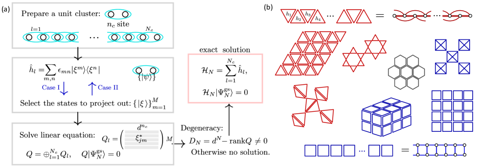
Figure 1: (a) Cluster-entangling scheme to construct a model that hosts an exact solution. Case I first determines $\hat{h}_{l}$ and obtain its excited states, $|\xi\rangle$, and Case II is vice versa. (b) Illustration of typical lattice models constructed as a sum of unit clusters: zigzag ladder, ladder, triangular lattice, kagome lattice, pyrochlore lattice, and square lattice. Usually, however, the corner-shared lattices in two and three dimensions are difficult to treat because of the small number of constraints $M$.

II Designing a Hamiltonian with exact ground state solutions

II.1 Essence of the framework

We first illustrate the essense of the present framework by using a well-known AKLTAffleck et al. (1987) state, although most of the states we discuss are far more complex and are not written down in a simple analytical form like AKLT. Let us consider a unit consisting of $n_{c}$ sites, where each site carries $d$ degrees of freedom. A sufficiently large finite-size system consisting of $N$ sites is regarded as an assembly of $N_{c}$ clusters, sharing their $n_{\cap}(<n_{c})$ sites with its neighbors.

Our goal is to construct a bulk quantum state on a finite but sufficiently large $N$ site cluster, $|\Psi_{N}^{\rm gs}\rangle$, that serves as an exact ground state of a Hamiltonian written as a sum of positive-definite operator $\hat{h}_{l}$ acting on the $l$-th cluster:

$${\cal H}_{N}=\sum_{l=1}^{N_{c}}\hat{h}_{l}.$$ (1)

The construction of $|\Psi_{N}^{\rm gs}\rangle$ is such that whenever we project this state onto any of the unit clusters by integrating out the $N-n_{c}$ part, they consist of a specified manifold of states $\{|\psi\rangle\}$ on the $l$-th cluster, satisfying $\hat{h}_{l}|\psi\rangle=0$. Here, the local Hibert space of a unit cluster has dimension $d^{n_{c}}$, which are classified by this penalty term $\hat{h}_{l}$ into two groups $\{|\psi\rangle\}$ and $\{|\xi\rangle\}$ of dimension $D_{g}$ and $M$, respectively, with $D_{g}+M=d^{n_{c}}$. If such $|\Psi_{N}^{\rm gs}\rangle$ is obtained, Eq.(1) becomes a so-called “frustration-free” Hamiltonian because the ground state energy is the sum of the lowest eigenvalues (zero) of $\hat{h}_{l}$.

The AKLT model serves as the most elementary example. Let the spin-1 chain be constructed from a site-shared spin-1 dimers with $n_{c}=2$ and $d=3$, where we need $N_{c}=N$ dimers for the periodic boundary condition (PBC) and $N_{c}=N-1$ for the cluster open boundary condition(C-OBC). For this unit, we may span the local Hilbert space of dimension 9 into four $S=0,1$ states as $\{|\psi^{m}\rangle\}_{m=1}^{4}$ and five $S=2$ states as $\{|\xi^{m}\rangle\}_{m=1}^{5}$, where we want to project out the latter. Using a projection operator ${\cal P}_{2}$ onto $S=2$, we obtain a local penalty Hamiltonian,

$$\hat{h}^{\rm AKLT}_{l}=\sum_{m=1}^{5}|\xi^{m}\rangle\langle\xi^{m}|={\cal P}_{2}(\bm{S}_{l}+\bm{S}_{l+1}).$$ (2)

By rewriting it using the spin-1 operator $\bm{S}_{i}$ and taking a sum over units, we reach the AKLT Hamiltonian:

$${\cal H}_{N}^{\rm AKLT}=\sum_{i=1}^{N}\frac{1}{2}(\bm{S}_{i}\cdot\bm{S}_{i+1})+\frac{1}{6}(\bm{S}_{i}\cdot\bm{S}_{i+1})^{2}+\frac{1}{3}.$$ (3)

The exact ground state $|\Psi_{N}^{\rm gs}\rangle$ that satisfies ${\cal H}_{N}^{\rm AKLT}|\Psi_{N}^{\rm gs}\rangle=0$ is known as AKLT state.

More generally, one can consider any $n_{c}$-site unit, making it share a site, an edge or a plane with its adjacent units, and design a lattice model and its exact ground state. Suppose that among $d^{n_{c}}$ states, the manifold of states $\{|\xi^{m}\rangle\}_{m=1}^{M}$, are designed to be projected out from the ground state. These states are orthogonal to the rest of the states $\{|\psi^{m^{\prime}}\rangle\}_{m^{\prime}=1}^{D_{g}}$ that constitute the ground state as, $\langle\xi^{m}|\psi^{m^{\prime}}\rangle=0$. We set $\hat{h}_{l}$ as a local penalty Hamiltonian written in the form,

$$\hat{h}_{l}=\sum_{m,n=1}^{M}\epsilon_{mn}|\xi^{m}\rangle\langle\xi^{n}|,$$ (4)

where the $M\times M$ matrix $\epsilon_{mn}$ should be positive semidefinite to have $|\xi^{m}\rangle$ as excited states.

However, determining $\hat{h}_{l}$ and $\{|\xi^{m}\rangle\}$ does not guarantee that we can obtain an exact eigenstate of ${\cal H}_{N}$. Unlike the exact AKLT state known a priori, we need to derive the actual form of $|\Psi_{N}^{\rm gs}\rangle$ that satisfies

$${\cal H}_{N}|\Psi_{N}^{\rm gs}\rangle=0.$$ (5)

Because one can always perform a Schmidt decomposition of any finite-size wave function into $l$-th cluster and the rest of the system of size $N-n_{c}$, whenever Eq.(5) holds, it means that there are no nonzero Schmidt values for $\{\xi\}$, in which case the ground state is expressed as

$$|\Psi_{N}^{\rm gs}\rangle=\sum_{m=1}^{D_{g}}\lambda_{m}|\psi^{m}_{l}\rangle|\Phi_{\bar{l}}^{m}\rangle,$$ (6)

where $\{|\Phi_{\bar{l}}^{m}\rangle\}$ is the Schmidt state on the rest of the system. This holds for both PBC and C-OBC. Operating $\hat{h}_{l}$ immediately gives Eq.(5). However, successively entangling $\{|\psi^{m}\rangle\}$ with those of their neighbors to make it fulfill Eq.(6) is not a promising task. Therefore, there can often be no solution that satisfies Eq.(5), in which case ${\cal H}_{N}$ is no longer called “frustration-free”. The core of our paper is the protocol given in Section II.2, that provides an unbiased and systematic construction of $\{|\Psi_{N}^{\rm gs}\rangle\}$ satisfying Eq.(5) or equivalently (6). In particular, this protocol is pinned down to the construction of MPS in the non-TI form in Sec.III.

It is known that for any given injective TI MPS, there always exists a frustration-free parent HamiltonianPerez-Garcia et al. (2007); Cirac et al. (2021). Its ground state is proved to be unique and has a finite gapPerez-Garcia et al. (2007). Here, we list the essential differences between our constructions.

• Our MPS tensors do not require TI form both for PBC and OBC and are constructed consecutively and independently between those of unconnected clusters by adding the clusters one by one. Whereas, the physical properties obtained from our MPS with PBC show TI, and those with OBC the symmetry about the center.

• The exact ground states $|\Psi_{N}^{\rm gs}\rangle$ very often show degeneracies both for PBC and OBC, where the former solution is included in the latter. Such degenerate solutions are difficult to access via DMRG using MPS as a variational ansatz.

• The corresponding frustration-free Hamiltonian can belong to the classes not only of gapped ground states but of gapless ground states and also those with long-ranged entanglement properties.

Although the frustration-free Hamiltonian is constructed from any given TI MPS, its vice versa, the way to derive the exact MPS ground state from the general frustration-free Hamiltonian was not mentioned beforePerez-Garcia et al. (2007); Cirac et al. (2021). The present protocol basically allows the latter for any frustration-free models in 1D and 2D for both PBC and OBC. In Table 1 we list such models whose ground states are established. We confirmed that for all these models, our method offers an exact MPS ground state at reasonable large $N$, e.g. see §.II.3 and §.IV. With this in mind, there are two strategies in choosing $\hat{h}_{l}$ and $\{\xi^{m}\}$.

Case I refers to when we are given the form of $\hat{h}_{l}$ and ${\cal H}_{N}$ we want to solve; We first check whether $\hat{h}_{l}$ has $D_{g}\geq 2$, otherwise we only have a trivial product ground state. When $D_{g}\geq 2$, by applying the protocol in §.II.2, we examine whether Eq.(5) is satisfied and if yes (i.e. $D_{N}\neq 0$ in Eq.(10)), we find that ${\cal H}_{N}$ is frustration-free and obtain its exact ground state.

Case II is when we want to search for an unknown Hamiltonian (see §.V for demonstration). We vary the choice of cluster states $\{|\xi^{m}\rangle\}_{m=1}^{M}$ as well as the way of overlapping the clusters $n_{\cap}$ to find the condition that satisfies Eq.(5). Once the condition is fulfilled, the form of ${\cal H}_{N}$ is determined through Eqs.(4) and (1).

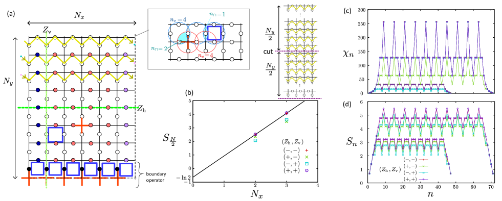
Figure 2: (a) Toric code in finite $N_{x}\times N_{y}$ size plaquettes including $N=2N_{x}N_{y}$ sites at the centers of the links. The red crosses and blue plaquettes indicate the projector $A_{v}$ and $B_{p}$ and the two green lines show the loop operators, $Z_{{\rm h}}$ and $Z_{{\rm v}}$. We color the sites depending on the types of projections imposed to determine their MPS tensor in constructing the MPS along the yellow 1D paths (partially shown on the upper part). (b) Entanglement entropy (EE) of the obtained exact MPS on four topological sectors for the division of the system into half, $S_{N/2}$, given as a function of circumferences $N_{x}$ at $N_{y}=12$. (c) Bond dimension $\chi_{n}$ and (d) EE, $S_{n}$, for the bipartition into the first $n$ site and the rest $N-n$, for four different topological sectors with $(N_{x},N_{y})=(2,12),(3,12)$.

II.2 Protocol for model construction

We start from an elementary method that straightforwardly imposes the condition Eq.(6) (equivalent to Eq.(5)) for all $l=1,\cdots,N_{c}$. It gives an exact ground state $|\Psi_{N}^{\rm gs}\rangle$ by solving a set of linear equations. Importantly, it tells us whether such an exact ground state exists or not, and if it exists, we find the number of degeneracy as well.

Suppose that we decide to project out $M$ different states on the $l$-th cluster, represented using the normalized and orthogonal set of $d^{n_{c}}$ basis $\{|j\rangle\}$ as

$$|\xi^{m}\rangle=\sum_{x=0}^{d^{n_{c}}-1}\tilde{\xi}^{m}_{x}|x\rangle.$$ (7)

with $\tilde{\xi}_{x}^{m}\in{\mathbb{C}}$. The elements of the local Hamiltonian in Eq.(4) is given as $\epsilon_{mn}=\sum_{x}\tilde{\xi}^{m}_{x}\tilde{\xi}^{n*}_{x}$. The local Hilbert space is classified as $\big{\{}\{|\psi^{m}\rangle\}_{m=1}^{D_{g}},\{|\xi^{m^{\prime}}\rangle\}_{m^{\prime}=1}^{M}\big{\}}$.

For the system size $N$ consisting of $N_{c}$ cluster, the Hilbert space dimension is $d^{N}$, and its subspace with $l$-th cluster state being restricted to $\{|\psi^{m}_{l}\rangle\}$ is defined as

$$V_{l}=\{\{|\psi_{l}^{m}\rangle\}\otimes|\Psi_{\bar{l}}^{j}\rangle_{j=0,\cdots,d^{N-n_{c}}-1}\},$$ (8)

where $\{|\Psi_{\bar{l}}^{j}\rangle\}$ is the space spanned by $N-n_{c}$ sites that do not belong to the $l$-th cluster.

The ground states belong to the subspace $V_{\rm gs}\equiv\cap_{l=1}^{N_{c}}V_{l}$. Projection to this state means imposing the following conditions on the whole Hilbert space: we prepare a $M\times d^{n_{c}}$ matrix using the coefficients of Eq.(7), $Q_{l}=(\tilde{\xi}^{m}_{x})$, and the conditions are described by the linear equation,

$$Q=\oplus_{l=1}^{N_{c}}Q_{l},\;\;\;\;Q|\Psi_{N}^{\rm gs}\rangle=0.$$ (9)

The number of rows of $Q$ is the total number of condition, $d^{N-n_{c}}MN_{c}$, and the number of columns is $d^{N}$. Solving this linear equation numerically gives the exact ground state when ${\rm dim}\cap_{l=1}^{N_{c}}V_{l}\neq 0$, and the degeneracy of the ground state is

$$D_{N}={\rm dim}\cap_{l=1}^{N_{c}}V_{l}=d^{N}-{\rm rank}Q.$$ (10)

Here, we mean by “exact”, not the analytical tractability (formula) of the wave function. It is natural because the wave functions always have ambiguity in the choice of phases or gauges, and also in the choice of the orthogonal sets when $D_{N}\geq 2$. Whereas, the exactness is guaranteed by machine epsilon as the types of local bases remaining are clearly separated from the rest of the Hilbert space by our rule, which makes the results numerically tractable.

Still, because the dimensions of $Q$ increase exponentially, there is an upper bound of $N$ that can be computed, which is comparable to the exact diagonalization scheme. This cost can be reduced by subsequently linking one cluster to another. We first prepare a single unit $N_{c}=1$, imposing a condition Eq.(7) to obtain a set of $\{\psi^{m}\}$ of dimension $D_{g}$. Then, add one unit cluster from another, where each time the condition to project the $d^{n}$ dimensional Hilbert space to $D_{n}$ solutions and the extra $M$ condition to project the states spanned on an added unit gives the number of rows of $Q$ as $D_{n}M$, which is reduced significantly from $d^{N-n_{c}}MN_{c}$.

The solutions can be classified by the symmetry of ${\cal H}_{N}$ represented by the operator ${\cal R}$. When the Hilbert space of the $n$ site system is divided into $r_{n}$-sectors by this symmetry, $\{R_{j}\}_{j=1}^{r_{n}}$, one can project the states onto these sectors at each process of adding a unit cluster, and obtain the eigenstate of both ${\cal R}$ and ${\cal H}_{N}$. We show the example in §.V.4.3.

In practice, we do not need to have large $N$ to judge whether the exact solution exists. The main usage of the protocol is to find a proper choice of $\{|\xi^{m}\rangle\}$ for a given cluster that yields a set of bulk Hamiltonian and the exact ground state. Once we confirm that there is a solution, we shall shift to the method in Section III, where the elements of the exact MPS representing $|\Psi_{N}^{\rm gs}\rangle$ are determined similarly to Eq.(9), that reaches far larger $N$ by the truncation which is nothing but the unitary transformation. It effiently chooses the basis, formally ”compressing the information” without sacrificing the exactness.

Figure 1(b) shows examples of the choices of unit clusters and the lattice that can be used in the present framework. The edge-shared lattices can be constructed both by the edge- and corner-sharing of clusters. However, the corner-shared units are not favorable for the present protocol in 2D as we see in §.IV because $M$ is relatively small and the number of solutions increases exponentially.

II.3 Revisiting AKLT and toric codes

Before going into the main results, we briefly show that the protocol successfully applies to the AKLT and toric code models.

For AKLT, we span a Hilbert space of spin-1 dimer as $\{|S^{z}_{l},S^{z}_{l+1}\rangle\}=(|1,1\rangle,|1,0\rangle,|0,1\rangle,|1,-1\rangle,|0,0\rangle,\cdots,|-1,-1\rangle)$ and classify them into $S=0,1$ and $S=2$ manifolds. The projection matrix $Q_{l}$ consists of Clebsch-Gordan coefficients of $S=2$ states,

$$Q_{l}=\left(\begin{array}[]{ccccccccc}1&0&\cdots&&&&&&0\\ 0&\frac{1}{\sqrt{2}}&\frac{1}{\sqrt{2}}&0&\cdots&&&&0\\ 0&0&0&\frac{1}{\sqrt{6}}&\frac{2}{\sqrt{6}}&\frac{1}{\sqrt{6}}&0&0&0\\ 0&\cdots&&&&0&\frac{1}{\sqrt{2}}&\frac{1}{\sqrt{2}}&0\\ 0&\cdots&&&&&&0&1\end{array}\right).$$ (11)

On the other hand, the MPS representation of the AKLT state for PBC is known as

$$|\Psi_{N}^{\rm AKLT}\rangle=\sum_{\{i_{n}\}}{\rm Tr}\big{(}\prod_{n=1}^{N}A^{i_{n}}\big{)}|i_{1},i_{2},\cdots,i_{N}\rangle,$$

$$A^{\pm 1}=\pm\frac{2}{\sqrt{3}}\sigma^{\pm},\;\;A^{0}=-\frac{1}{\sqrt{3}}\sigma^{z},$$ (12)

where $i_{n}=1,0,-1$ denotes $S_{n}^{z}$ on site $n$ and $\sigma$ is the Pauli matrix. The operation, $Q\,|\Psi_{N}^{\rm AKLT}\rangle=0$, in Eq.(9) corresponds to having

$$A^{1}A^{1}=0$$

$$A^{1}A^{0}+A^{0}A^{1}=0$$

$$A^{1}A^{-1}+2A^{0}A^{0}+A^{-1}A^{1}=0$$

$$A^{-1}A^{-1}=0,$$ (13)

which is confirmed straightforwardly. We can also check that in the case of OBC, the number of degeneracies is four that explains the number of edge states.

We now demonstrate briefly how the $\mathbb{Z}_{2}$ quantum spin liquid ground state of the toric code Kitaev (2003) is described by our MPS (for the derivation see §.III and IV). The Hamiltonian consists of vertex ($A_{v}$) and plaquette ($B_{p}$) operators summed over the system as

$$\mathcal{H}_{{\rm toric}} =-\sum_{v}A_{v}-\sum_{p}B_{p},$$

$$A_{v}=\prod_{i\in v}\sigma^{x}_{i},\quad B_{p}=\prod_{i\in p}\sigma^{z}_{i}.$$ (14)

All $A_{v}$’s and $B_{p}$’s commute and have eigenvalues $\pm 1$, so that the ground state will be the simultaneous $+1$ eigenstate of all the operators which makes Eq.(14) frustration-free. In applying our protocol, we prepare two species of clusters both with $n_{c}=4$, given in blue and red circles in the inset of Fig. 2(a), which have overlap $n_{\cap}=1$ and 2 between the same and different species, respectively. The local penalty Hamiltonians for the two clusters are $\hat{h}_{l}=A_{v}$, $B_{p}$, and the corresponding $Q_{l}$ in Eq.(9) is set to project out from among $2^{4}$ states the $M=8$ states with eigenvalue $-1$ of $\hat{h}_{l}$.

To prepare a torus based on $N_{x}\times N_{y}$ plaquettes ($N=2N_{x}N_{y}$), we wrap them by drawing the spiral 1D MPS path running along the $x$-direction as shown in Fig. 2(a). We add the MPS tensors one by one from top left to bottom right and determine their elements by performing a projection as follows (for details see §.III): the MPS tensor of the blue-colored site is determined by $Q_{l}$ giving $B_{p}=1$ on the upper plaquette that makes PBC in the $x$-direction. The red-colored site is imposed $A_{v}~{}=1$ on the left and $B_{p}=1$ on the upper plaquette, the purple site by imposing two $A_{v}=1$ and one $B_{p}=1$, and otherwise, no projection is given. To form a torus, the PBC in the $y$ direction is attained by diagonalizing the boundary operator, ${\cal H}^{\text{bd}}=-\sum_{j=1}^{N_{x}}(A_{v\in(j,N_{y})}+B_{p\in(j,N_{y})})$, consisting of operators on the last row. We find $D=4$ fold degenerate eigenstates with eigenvalue $-2N_{x}$. Finally, we apply two loop operators $Z_{{\rm h}}=\prod_{i\parallel x}\sigma^{z}_{i},\;Z_{{\rm v}}=\prod_{i\parallel y}\sigma^{z}_{i}$, running along the closed horizontal and vertical paths, respectively, which classify the four degenerate ground states into topological sectors by their eigenvalues $\pm 1$. (For bounary and spring operators we apply the third method in §.III.3).

Figure 2(b) shows the entanglement entropy(EE) $S_{N/2}$ for cutting the torus into half; given an extrapolation by an area of a cut (curcumference) $N_{x}\rightarrow 0$, they clearly show the extrapolation to the $-\ln 2$ value known as the topological EE of a ${\mathbb{Z}}_{2}$ spin liquidJiang et al. (2012).

Our MPS does not have TI as can be seen from the bond dimension and the EE when we divide the system into $n$ and $N-n$ sites in Figs. 2(c) and 2(d) for four different topological sectors and $(N_{x},N_{y})=(2,12),(3,12)$, namely $N=48,\;72$. The bond dimension depends on the place of a cut as $\hat{h}_{l}$ is imposed in a period of $N_{x}$, where we find that the maximum bond dimension required to have a toric code is given as $\chi_{n}\lesssim 100N_{x}$, which is feasible for standard numerical resources.

We finally list several advantages of getting an exact toric code ground state. Previous numerical approximations using DMRG working on cylinders naturally select minimally entangled states, which are the superposed ones from the $\pm$ topological sectors, underestimating EEJiang et al. (2012, 2013). It is indeed generally difficult to obtain the topologically degenerate states of all sectors independently, as the eigenstates of the loop operators are found difficult to identifyCincio and Vidal (2013); He et al. (2014). Our method can elucidate them easily, and can further identify all the excited states exactly by converting arbitrary sets of $\{A_{v},B_{p}\}$ as $-1$.

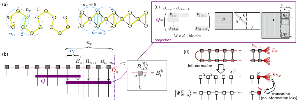
Figure 3: (a) Examples of lattices with a choice of $n_{c}=5,n_{\cap}=2$. (b) Schematic illustration to construct the exact MPS. In and outward arrows indicate the order of determining the elements of $B_{n}$ using the projection matrix $Q$. These elements are obtained by the singular value decomposition of $Q$. (c) Process of determining $B_{n+n_{a}}$ at step 1 and 2 by the projection matrix $Q$, where we perform the SVD. (d) Processes in step 4 and 5; left-normalization and the process of extracting $p=1,\cdots,D_{N}$ independent $|\Psi_{N,p}^{\rm gs}\rangle$. The SVD is performed from right to left to reduce the bond dimensions to sufficient values $\chi_{n}$.

III Exact Matrix product solutions

In this section, we present the actual process of zeroing out part of the subspace of each cluster in determining the elements of the MPS tensor. This is done by successively adding the tensor and imposing projectors. The advantage of using MPS representation is that it could ”compress” the information without losing the exactness, relying on the canonical form and orthogonalization. The MPS is used not as a variational ansatz but as a convenient form of storing full information on the wave functions.

III.1 Cluster-open boundary MPS in one dimension

In our protocol introduced in §.II the maximum system size $N$ available was limited by the substantial growth of dimension of the Hibert space and the number of conditions. Here, we extend the method by adopting the MPS wave function. As we saw in Eq.(13), the matrices $A^{(i_{n})}$ of the AKLT state fulfill the exact-solution condition of the protocol, from which we can anticipate that other states can be similarly treated. Regardless of the model, the form of MPS for OBC is given as

$$|\Psi_{\rm gs}\rangle=\sum_{i_{1},i_{2},\cdots,i_{N}=1}^{d}A^{[1]i_{1}}_{1\beta_{1}}A^{[2]i_{2}}_{\alpha_{2}\beta_{2}}\cdots A^{[N]i_{N}}_{\alpha_{N}1}\;|i_{N}\cdots i_{1}\rangle,$$ (15)

where $A^{[n]i_{n}}_{\alpha_{n}\beta_{n}}$ has a dimension $\chi_{n-1}\times\chi_{n}\times d$. We determine the size and elements of these matrices.

As a preparation, we choose a unit cluster consisting of $n_{c}$ sites and decide how to construct the lattice by making the neighboring clusters share $n_{\cap}(<n_{c})$ sites. In Fig. 3(a) we show two example of the constructions of lattices with $n_{c}=5$ and $n_{\cap}=2$ to guide the following explanation. We consider a 1D system with C-OBC which is the OBC of clusters, not the sites. Compared to standard OBC, half of the interactions among $n_{\cap}$ sites belonging to $\hat{h}_{1}$ and $\hat{h}_{N_{c}}$ are lacking. We decide the 1D path of MPS on the lattice, e.g. as shown in bold lines in Fig. 3(a).

Next, we obtain a series of matrices $\{B_{\alpha_{n}\beta_{n}}^{i_{n}}\}_{n=1}^{N}$ as shown in Fig. 3(b), which is written simply as $B_{n}$, mk and finally derive $A_{n}$ from $B_{n}$. These processes are performed following the steps given below. Further details are provided in the next subsection.

• Obtain $B_{1},\cdots,B_{n_{c}}$ as an initial set of MPS. We first diagonalize the $n_{c}$-site unit cluster and from among the eigenstates, choose $M$ states $\{\xi^{m}\}$ that is to be projected out, expressed in the form of Eq.(7), which give the element of $Q$. We can choose a general form of $B_{1},\cdots,B_{n_{c}-1}$ using a set of unit matrices, whose bond dimensions are $D_{n}=d^{n}$. Using $B_{1},\cdots,B_{n_{c}-1}$, we decide the form of $B_{n_{c}}$ that projects out $\{\xi^{m}\}$ by the singular value decomposition (SVD) of matrix $Q$ (see Fig. 3(c)). The final bond dimension is $D_{n_{c}}=D_{g}=d^{n_{c}}-M$.

• Add $n_{a}\equiv n_{c}-n_{\cap}$ successive sites (one cluster) to have $n^{\prime}=n+n_{a}$ system. Again the $B_{n}$ of the first $n_{a}-1$ sites are obtained by the unit matrices. When adding the last site, we again construct a matrix $Q$ that fulfills the linear equation for projection to the cluster ground state. The SVD of $Q$ will provide $B_{n^{\prime}}$ of dimension $D_{n+n_{a}}$.

• Repeat step 2 by setting $n^{\prime}$ as updated $n$ until we reach the system size $n^{\prime}=N$. The final matrix has dimensions $D_{N-1}\times D_{N}\times d$. A set of matrices $\{B_{n}\}_{n=1}^{N}$ represents $D_{N}$ degenerate solutions.

• We left-normalize a sets of matrices $\{B_{n}\}_{n=1}^{N}$ to make them orthogonal.

• We divide the matrix $B_{N}$ into $D_{n}$ columns. The $D_{n}$ independent solutions are these column vectors combined with $\{B_{n}\}_{n=1}^{N-1}$ common to all of them. For each such set, we start from right $n=N-1$ toward $n=1$ and truncate the matrix. At each step, we divide the system into $n$ and right $N-n$ matrices and perform a Schmidt decomposition to discard the bonds that have zero Schmidt values which reduces the bond dimensions to $\chi_{n}$. $\{B_{n}\}_{n=1}^{N}$ is converted to $\{A_{n}\}_{n=1}^{N}$.

When we consider the 1D system, we often find the case that the truncation in step 5 is needed for only the right half of the system, namely $\chi_{n}=D_{n}$ and $A_{n}=B_{n}$ for $n=1,\cdots N/2$. However, in general, the truncation is given throughout the system. The truncation here is not losing information but shrinks the bond dimension by discarding the idle dimension. This is because, the series of nonzero Schmidt basis are exactly determined, and the growth of $D_{n}$ beyond $\chi_{n}$ is simply because the former is not taken in the optimal canonical form. In that respect, the present MPS solutions are numerically precise in machine epsilons, beyond those of the exact diagonalization calculation in practice.

We finally briefly show the implication of step 5 (see Fig. 3(d)). We truncate the bond dimensions of matrix of $D_{n}$ of $B_{n}^{i}$ to $\chi_{n}$ of $A_{n}^{i}$ one by one. Let the matrix be described as an assembly of column vectors of dimension $\chi_{n-1}$ as $B_{n}^{i}=(\bm{b}_{n,1}^{i},\cdots,\bm{b}_{n,\chi_{n}}^{i})$. Left-normalization imposed on these matrices indicates,

$$\sum_{i=1}^{d}B_{n}^{i\dagger}B_{n}^{i}=\hat{I}_{\chi_{n}},$$

$$\sum_{i=1}^{d}\bm{b}_{n,p}^{i\dagger}\bm{b}_{n,q}^{i}=\delta_{pq},$$ (16)

wher $\hat{I}_{n}$ is the unit matrix of dimension $n$. From among the $D_{N}$ bonds on the rightmost matrix $B_{N}$, choosing the $p$-th column vector $\bm{b}_{N,p}$, we find the $p$-th ground state $|\Psi_{N,p}^{\rm gs}\rangle$. Because of Eq.(16), for $p,q=1,\cdots,D_{n}$,

$$\langle\Psi_{N,p}^{\rm gs}|\Psi_{N,q}^{\rm gs}\rangle=\bm{b}_{N,p}^{\dagger}\bm{b}_{N,q}=\delta_{pq},$$ (17)

holds, namely, the degenerate ground states are orthogonal to each other. Unlike $B_{n}^{i}$, the $A_{n}^{i}$ obtained after the truncation for $n=1,\cdots,N-1$ are no longer common among $D_{N}$ degenerate solutions.

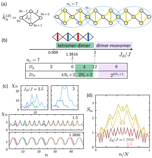
Figure 4: Application of MPS approach to the spin-1/2 Heisenberg diamond chain. (a) Unit Hamiltonian and the lattice we use for the construction of MPS ($n_{c}=7$, $n_{\cap}=1$, C-OBC). (b) The ground state phase diagram Takano et al. (1996) with two exact solutions, tetramer-dimer and dimer-monomer states, with energies $E=n_{v}(e_{t}+e_{s})$ and $n_{v}e_{s}$, respectively, where $e_{t}=2(-J+J_{d}/8)$ and $e_{s}=-3J_{d}/4$ are the energies of rung-triplet and rung-singlet state per diamond. For $n_{c}=7$, $\hat{h}_{l}$ has several $D_{g}$ degeneracies. The exact solutions are available at $J_{d}/J\geq 1.386$ with $D_{g}>2$. (c) Bond dimension $\chi_{n}$ for $J_{d}/J=1.3816,1.5,2,2.5$ where we take $N=7,13,19,\cdots,45$. (d) Bipartite entanglement entropy $S_{n}$ for corresponding data of panel (c), where we select $N=49$ and $19$, which are the reasonable maximum size available for given $D_{g}$. Data of (c) and (d) are averaged over all degenerate ground states.

III.2 Example: spin-1/2 diamond chain

We demonstrate the process proposed in the previous subsection in the spin-1/2 diamond chain shown in Fig. 4(a). Two exact solutions for the Heisenberg model with two coupling constants, $J$ and $J_{d}$, are knownTakano (1994); Takano et al. (1996), which are the tetramer-dimer and dimer-monomer states as shown in the phase diagram of Fig. 4(b). Deriving the corresponding MPS for these states refer to Case I in Fig. 1(a) where $\hat{h}_{l}$ is given á priori. The unit cluster to accommodate all these states without bias is $n_{c}=7$, namely two diamonds, which share $n_{\cap}=1$ with its neighbor. Notice that we may also choose $n_{c}=4$ (one diamond) and apply two different projections alternatively to simply obtain part of these states, which we do not adopt here.

For each diamond we have a Heisenberg Hamiltonian $\hat{h}^{(d)}_{n}$ and the cluster Hamiltonian is given as

$$\hat{h}_{l}=\hat{h}^{(d)}_{2l}+\hat{h}^{(d)}_{2l+1},$$

$$\hat{h}^{(d)}_{n}=J(\bm{s}_{3n-1}+\bm{s}_{3n})(\bm{s}_{3n-2}+\bm{s}_{3n+1})+J_{d}\bm{s}_{3n-1}\bm{s}_{3n+1}.$$ (18)

We denote the down and up spin state $s_{n}^{z}=\mp 1/2$ for each site as $i_{n}=0$ and $1$, respectively, and describe the $n$-spin state as $|i_{n}i_{n-1},\cdots i_{1}\rangle$, e.g. $|0100\cdots\rangle$ given in the descending order of site indices. These states are indexed by $x=0,\cdots 2^{n}-1$ which is the base-ten numerals of these bits. For example, in diagonalizing Eq.(III.2) at $J_{d}/J=1.5$, we have $D_{g}=4$ fold degenerate lowest energy state, and we need to project out $M=2^{7}-4=128$ states per cluster.

Let us explain the details of step 1 ($n=0$) and step 2 ($n>n_{c}$). At both steps, we add $n_{a}$-sites ($n_{a}=n_{c}=7)$ for the initial step 1 and $n_{a}=n_{c}-n_{\cap}=6$ for successive step 2 and we need to obtain $B_{n+1},\cdots B_{n+n_{a}}$. For the first $n_{a}-1$ sites, the matrices describe the full set of basis $2^{n_{a}-1}$ equivalently, and are given by the disaggregation of unit matrix, $\hat{I}$. For $B_{n+1}$, by dividing the $2\times 2$ unit matrix into upper and lower parts, we find $B_{n+1}^{0}=\hat{I}_{D_{n}}\otimes(1\>0)$ and $B_{n+1}^{1}=\hat{I}_{D_{n}}\otimes(0\>1)$. The second site matrices are given by dividing the $4\times 4$ into two $2\times 4$ as $B_{2}^{0}=I_{D_{n}}\otimes(1\>0\>0\>0;0\>1\>0\>0)$ and $B_{2}^{1}=I_{D_{n}}\otimes(0\>0\>1\>0;0\>0\>0\>1)$. We successively construct the rest of them up to $n+n_{a}-1$.

For $B_{n+n_{a}}$ we impose the condition to project out $\{|\xi^{m}\rangle\}$. The basis of $n_{c}$-site cluster is $|x\rangle=|i_{n_{c}}i_{n_{c}-1}\cdots i_{1}\rangle$, having $M$ different excited states, Eq.(7). Next, for each of $m=1,\cdots,M$ different conditions, we prepare $D_{n}\times D_{n+n_{a}-1}$ matrix for $i_{n+n_{a}}=0,1$

$$P_{m;i_{n+n_{a}}}\!=\!\sum_{x=0}^{2^{n_{a}-1}}\tilde{\xi}^{m}_{x}\big{(}B^{i_{n}}_{n}B^{i_{n+1}}_{n+1}\cdots B^{i_{n+n_{a}-1}}_{n+n_{a}-1}\big{)}.$$ (19)

Using them we construct a projection matrix of $(MD_{n-1})\times(dD_{n+n_{a}-1})$, with $d=2$ as

$$Q=\left(\begin{array}[]{ll}P_{1;0}&P_{1;1}\\ \vdots\\ P_{M;0}&P_{M;1}\end{array}\right),\quad Q\>\bm{v}_{b}=0,$$ (20)

where $\bm{v}_{b}$ has dimension $(dD_{n+n_{a}-1})$. To obtain such $\bm{v}_{b}$ we perform a SVD as $Q=U\Lambda V$, where $\Lambda$ has at most ${\rm min}(dD_{n+n_{a}-1},MD_{n})$ nonzero diagonal values. This means that the $D_{n+n_{a}}$ rightmost columns of matrix $V$ serve as different $\bm{v}_{b}$. A set of matrices, $B_{n+n_{a}}^{1}$ to $B_{n+n_{a}}^{d}$, are obtained by dividing the $(dD_{n+n_{a}-1})\times D_{n+n_{a}}$ part of $V$ into $d$-blocks with $D_{n+n_{a}-1}\times D_{n+n_{a}}$. These processes are shown schematically in Fig. 3(c).

We finally briefly explain the results obtained. Takano,et.al found the exact tetramer-dimer ground state at $J_{d}/J\lesssim 2$Takano et al. (1996). On a single diamond, the triplet on a rung and the other triplet based on two sides entangle and form a tetramer, which has the energy $e_{t}=2(-J+J_{d}/8)$. On its neighbor, the singlet resides on a rung with energy $e_{s}=-3J_{d}/4$. The total energy of the product states of tetramer and dimer is given by $E=(e_{t}+e_{s})n_{v}/2$ where $n_{v}$ is the number of rungs. Numerically, the ground state energy is found to extrapolate to $E/N$ smoothly with increasing $N$ at $0.909<J_{d}/J<2$. However, our method shows that there is another point, $J_{d}/J=1.3816$, not reported previously, that exhibits the energy crossing of the $n_{c}=7$ cluster Hamiltonian $\hat{h}_{l}$. One possibility is that $J_{d}/J=1.3816$ is a phase transition point. However, below this point, the ground state degeneracy of $\hat{h}_{l}$ is $D_{g}=2$ and we cannot find an exact solution. Another possibility is that the trimer-dimer ground state of the form of restricting the population of states per diamond is no longer an exact but an approximate ground state at $J_{d}/J<1.3816$. In such cases, a larger inter-cluster fluctuation including excited states needs to be taken into account which is numerically hard to access.

In Figs. 4(c) and 4(d), we show the bond dimension of MPS and the bipartite entanglement entropy $S_{n}$ when dividing the system into $n$ and $N-n$ parts. We find that the case of $J_{d}/J=1.3816$ and $1.5$ are similar in $S_{n}$ and are nearly flat, consistent with the product nature of the ground state. However, the profile of $\chi_{n}$ differs much, which may suggest the change of the nature of the ground state below 1.3816. The other two cases with larger $D_{g}$ show a significant increase of $\chi_{n}$ and $S_{n}$, showing that our method can be a fingerprint of elucidating the nature of the phases.

The extension of diamond chain exact solutions to 2D diamond lattice was reportedMorita and Shibata (2016), hosting a highly degenerate ground state because of an arbitrarity of choosing the dimer covering pattern. Such a case can also be dealt with in our framework if we set the projection to be the tetramer or dimer singlet states for $n_{c}=4$ diamond and apply a 2D scheme in §.IV.

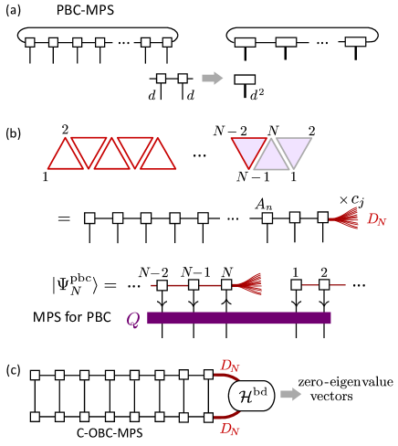
Figure 5: (a) Construction of 1D PBC-MPS using projection matrix $Q$. The right panel is the $k=\pi$ PBC-MPS. (b) Construction of MPS for PBC Hamiltonian that applies the same method for C-OBC MPS by adding projections about the two triangles at the boundary. (c) PBC-MPS obtained by diagonalizing $\mathcal{H}^{\rm bd}$, which is the most practical.

III.3 MPS for the periodic boundary Hamiltonian in one dimension

The MPS that applies to the Hamiltonian with periodic boundary condition (PBC) takes the form

$$|\Psi_{N}^{\rm pbc}\rangle=\sum_{\{i_{n}\}}^{d}{\rm tr}\big{(}\tilde{A}^{i_{1}}_{1}\cdots\tilde{A}^{i_{N}}_{N}\big{)}|i_{N}\cdots i_{1}\rangle.$$ (21)

It is known that for a given OBC-MPS, one can construct a PBC-MPS with bond dimensions increased by a factor of $N$ Perez-Garcia et al. (2007); for each local degree of freedom, $i=1,\cdots d$, we combine a set of $\{A_{n}\}$ on the $(n,n+1)$ block as

$$A^{{\rm pbc};i}=N^{-1/N}\left(\begin{array}[]{llllc}0&A_{1}^{i}&0\cdots&&0\\ 0&0&A_{2}^{i}&\\ \vdots&&&\ddots\\ 0&\cdots&&&A_{N-1}^{i}\\ A_{N}^{i}&0\cdots&&&0\\ \end{array}\right),$$ (22)

which allows a newly obtained matrix of the form,

$$\sum_{\{i_{n}\}}{\rm tr}\big{(}\prod_{n=1}^{N}A^{{\rm pbc};i}_{n}\big{)}|i_{N}\cdots i_{1}\rangle$$

$$=\frac{1}{N}\sum_{j=0}^{N-1}\sum_{\{i_{n}\}}^{d}{\rm tr}\big{(}A^{i_{1}+j}_{1}\cdots A^{i_{N}+j}_{N}\big{)}|i_{N}\cdots i_{1}\rangle,$$ (23)

which fulfills the translational invariance, and formally reduces to Eq.(21). Such PBC-MPS is the eigenstate of the translation operator ${\cal T}$ and we can design it to have ${\cal T}|\Psi_{N}^{\rm pbc}\rangle=e^{ik}|\Psi_{N}^{\rm pbc}\rangle$. For example, when $k=\pi$, we combine two matrices as $(B_{n}^{i}\otimes B_{n+1}^{i})$ and prepare Eq.(22) for $N/2$ blocks (see Fig. 5(a)). However, since the OBC-MPS (which includes C-OBC) in our case is degenerate, they naturally generate only part of the PBC-MPS, and does not guarantee the completeness of the solution. Another drawback is that the method requires more bond dimensions than necessary.

We now propose three practical ways to obtain a full set of MPS for the PBC Hamiltonian that overcomes the above issues.

Imposing projection. This method does not differ much from the treatment of constructing C-OBC-MPS in §.III.1. We explain the difference using the zigzag ladder based on triangles in Fig. 5(b). The PBC Hamiltonian is realized from the C-OBC one by adding one triangle and connecting the edge sites. We follow step 1 and consecutively apply step 2 for $n=1,\cdots,N-2$ until we reach the last cluster. At the final step, we first add $B_{N-1}$ using the unit matrix, and then derive $B_{N}$ by simultaneously imposing three projection matrix $Q$ that operate on $(N-2,N-1,N)$, $(N-1,N,1)$, and $(N,1,2)$ triangles. We then apply steps 4 and 5 and obtain $\tilde{D}_{N}$ degenerate solutions forming the columns of $\tilde{A}_{N}$. The two extra $Q$ required reduces the bond dimension to $\tilde{D}_{N}<D_{N}$.

Translation operator.    In deriving MPS for the PBC Hamiltonian, one can directly classify them by an operator ${\cal T}$, that shifts the wave function by one lattice spacing along the 1D path of the MPS, where we assume that the $n=N$ site is put back to $n=1$. We first prepare a full set of OBC-MPS, $\{|\Psi_{N,j}^{\rm gs}\rangle\}$, obtained in §.III.1. Then, we evaluate the matrix representation of $\langle\Psi_{N,j}^{\rm gs}|{\cal T}|\Psi_{N,k}^{\rm gs}\rangle$ of dimension $D_{N}$ and by diagonalizing it, the $\tilde{D}_{N}$ different PBC-MPS is obtained as its eigenstates. Suppose that $l$-th eigenvector of ${\cal T}$ is $(c_{1}^{(l)},\cdots,c_{D_{N}}^{(l)})$, which means

$$|\Psi_{N}^{{\rm pbc};(l)}\rangle=\sum_{j=1}^{D_{N}}c_{j}^{(l)}|\Psi_{N,j}^{\rm gs}\rangle,$$ (24)

and using the column vectors of $B_{N}^{i}=(\bm{b}_{N,1}^{i},\cdots,\bm{b}_{N,D_{N}}^{i})$, the $l$-th PBC-MPS solution of dimension $\chi_{N-1}\times 1$ yields,

$$\tilde{B}_{N}^{i}=\sum_{j=1}^{D_{N}}c_{j}^{(l)}\bm{b}_{N,j}^{i}.$$ (25)

The rest of the truncation process in step 5 is the same as before.

Diagonalizing the boundary operator.

Evaluating the matrix representation of the spin operator is easier than using $\mathcal{T}$ since there is no efficient matrix product operator (MPO) representation of the translation operator. We first divide the Hamiltonian by the C-OBC term and the boundary term, given as

$$\mathcal{H}_{N}=\mathcal{H}^{\text{C-OBC}}_{N}+\mathcal{H}^{\rm bd}.$$ (26)

Then we prepare a full set of OBC-MPS $\{|\Psi^{\rm gs}_{N,j}\rangle\}$ and diagonalize the boundary term, $\langle\Psi_{N,j}^{\rm gs}|\mathcal{H}^{\rm bd}|\Psi_{N,k}^{\rm gs}\rangle$, given in the form of $D_{N}\times D_{N}$ matrix as shown schematically in Fig. 5(c). The number of zero eigenvalues is the degeneracy of the PBC ground states, and by using the eigenvectors, the PBC-MPS is constructed using Eqs. (24) and (25). This method is the most efficient among the three, allowing for larger $N$. For example, in constructing the PBC-MPS of the zigzag chain (see state E in Fig. 10(a) in §.V), we could reach up to $N=18$ for the method of imposing projection, while for diagonalizing $\mathcal{H}^{\rm bd}$ we find up to $N=40$, and find $D^{\rm PBC}_{N}=50$ degenerate PBC solutions out of $D_{N}=441$ C-OBC solutions.

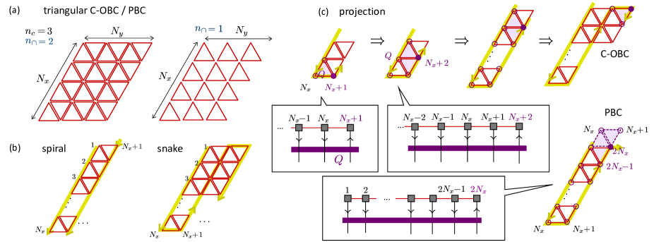
Figure 6: Construction of 2D MPS. (a) Triangular lattice of $N=N_{x}\times N_{y}$ sites using $n_{c}=3$ cluster with site overlaps, $n_{\cap}=2$ and $n_{\cap}=1$. (b) Spiral and snake type 1D path for constructing MPS. (c) How we operate the projection matrix $Q$ at each step for the snake type MPS and for PBC. Bullet indicates the $n$-th site which we want to determine $B_{n}$ by the projection $Q$. The matrix $Q$ includes several triangles highlighted in purple where we want to exclude $\{\xi^{m}\}_{m=1}^{M}$, and also includes the information of matrices of the open circles that are not even included in the projected triangles. When we apply PBC in the $x$-direction, we need to make projections at $n=2N_{x}$ about three triangles with inputs from $2N_{x}-1$ sites that share the first and second columns of the lattice. In constructing a cylinder, we set the PBC in the $x$-direction that the snake runs.

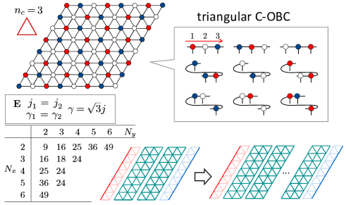
Figure 7: Results obtained for a parameter $\gamma=\sqrt{3}j$ with regular triangular geometry in Eq.(32) corresponding to point E. Unlike the zigzag chain $\Gamma=\sqrt{3}J(=2\gamma)$ is also a regular triangle inside the lattice cluster. The degree of degeneracy of the ground state(bottom panel), and the three sublattce ground state whose MPS state consists of 9 tensors shown here. The lattice size is expanded by making three columns per unit as blocks.

IV Exact matrix-product-states in two-dimensional and random cases

IV.1 Construction of two dimensional MPS

The construction of MPS we showed in §.III is straightforwardly extended to 2D, while several points differ from 1D, as one may anticipate from the brief demonstration for the toric code presented in §.II.3. For comprehensiveness, we consider the triangular unit $n_{c}=3$ as shown in Fig. 6(a): we can choose either $n_{\cap}=2$ and $1$ depending on how we design the boundary conditions and numerical costs. There are spiral or snake-type 1D paths of constructing MPS as shown in Fig. 6(b), while we here adopt the latter; At $n=N_{x}+1$ we only need to include a single triangle for projection. However, from $n=N_{x}+2$ to $2N_{x}-1$, we need to include two triangles highlighted and the input from the related sites marked with open circles. This is because the dimensions of matrices differ between sites that are separated to long distance over the MPS path, and we need to track the intervals to contract them. Besides the C-OBC, we can also construct a cylinder by taking PBC in the $x$-direction, in which case we need to project out the excited states of three triangles at $n=2N_{x}$ with input from $2N_{x}-1$ sites. The schematic illustration of constructing MPS is shown together in Fig. 6(c).

IV.2 Two dimensional MPS on a triangular lattice

We now construct MPS with $n_{c}=3,n_{\cap}=2$ for the triangular lattice of size $N=N_{x}\times N_{y}$ with C-OBC whose details are shown in Fig. 7. We select the $M=2$ states the same as for the zigzag chain in §.V, i.e. Eq.(31), and study the cluster Hamiltonian of the form Eq.(32). The bonds on the edges of the rectangle have half the values of coupling constants as those inside. When considering the AF-XXX-$\Gamma$ model, $j_{1}=j_{2},\gamma_{1}=\gamma_{2}$ with $\gamma/j=\sqrt{3}$ (E) where the triangular unit has a $C_{3}$ symmetry, we find $D_{N}$ as shown in the lower panel. Here, either $N_{x}$ or $N_{y}=2$ case corresponds to the zigzag chain. The same degeneracy is found for other $C_{3}$ case ($\cos\beta=1/\sqrt{3}$) as well as for $j_{2}/j_{1}=-1/4$ and $\gamma=0$ (D).

Most of these degenerate ground states have a perfect three-sublattice geometry about $\langle S_{j}^{z}\rangle$, while the values of $\langle S_{j}^{z}\rangle$ of three different colored sites can vary without changing the energy. We also found that the matrices of such ground states consist only of nine elements shown in Fig. 6(c): the top three matrices are the constituents that do not cross the boundary. These states are product states and indeed, if we divide for example the $8\times 8$ lattice into four parts and duplicating the inner two (which are identical in terms of the distribution of bond dimensions), increase the lattice size, which gives exactly the ground state energy of $E=-3JN/4$. In performing parallelly the DMRG calculation, the bond dimensions turned out to be much more suppressed down to $\chi_{n}=3,4$ for up to $N_{x},N_{y}=10$.

To explicitly construct the three-sublattice product ground state in our framework, we can define three different species of single-site states with indices $\gamma_{s}=a,b,c$ as

$$|\gamma_{s}\rangle=\cos(\theta_{\gamma_{s}}/2)e^{-i\phi_{\gamma_{s}}/2}|1\rangle+\sin(\theta_{\gamma_{s}}/2)e^{i\phi_{\gamma_{s}}/2}|0\rangle,$$ (27)

which are parameterized by $\theta_{\gamma_{s}}$ and $\phi_{\gamma_{s}}$. For a unit triangle with its ground state $|\psi\rangle=|a\rangle|b\rangle|c\rangle$, these parameters are set to fulfill $\hat{h}_{l}|\psi\rangle=0$. Here, the cluster Hamiltonian is predefined for the XXZ and $C_{3}$ cases as $\hat{h}_{l}=|\xi_{\Uparrow}\rangle\langle\xi_{\Uparrow}|+|\xi_{\Downarrow}\rangle\langle\xi_{\Downarrow}|$. We then find the ground state $|\Psi^{\rm gs}\rangle=\prod_{i=1}^{N}\otimes|\gamma_{s}\rangle_{i\in\gamma_{s}}$. For the XXZ case, this form does not conserve the total $S^{z}$ so we need to project the obtained states to the local Hilbert space of each total-$S^{z}$ sector, which gives the exact ground state.

The similar exact ground states are found in the kagome lattice for the XXZ model at $J_{z}=-1/2$ Changlani et al. (2018) and the XYZ model ($C_{3}$ line in our case) Palle and Benton (2021), where they constructed the three-coloring exact solutions as product state. In the kagome lattice, there is a macroscopic number of configurations of tiling the three-colored triangles unlike the triangular lattice with fixed three sublattices, and the number of degenerate solutions they derived relies on that degeneracy. However, the number of degeneracy can exceed the number of three colorings for a sufficiently large size of the lattice, which cannot be detected in their frameworks. Our method does not rely on this consideration and gives the unbiased exact degeneracy. In fact, for a zigzag ladder, a sawtooth chain, and a triangular lattice, the number of three-colorings is restricted to maximally three, while we can still find a substantial degeneracy in the ground state, which cannot be captured by intuition.

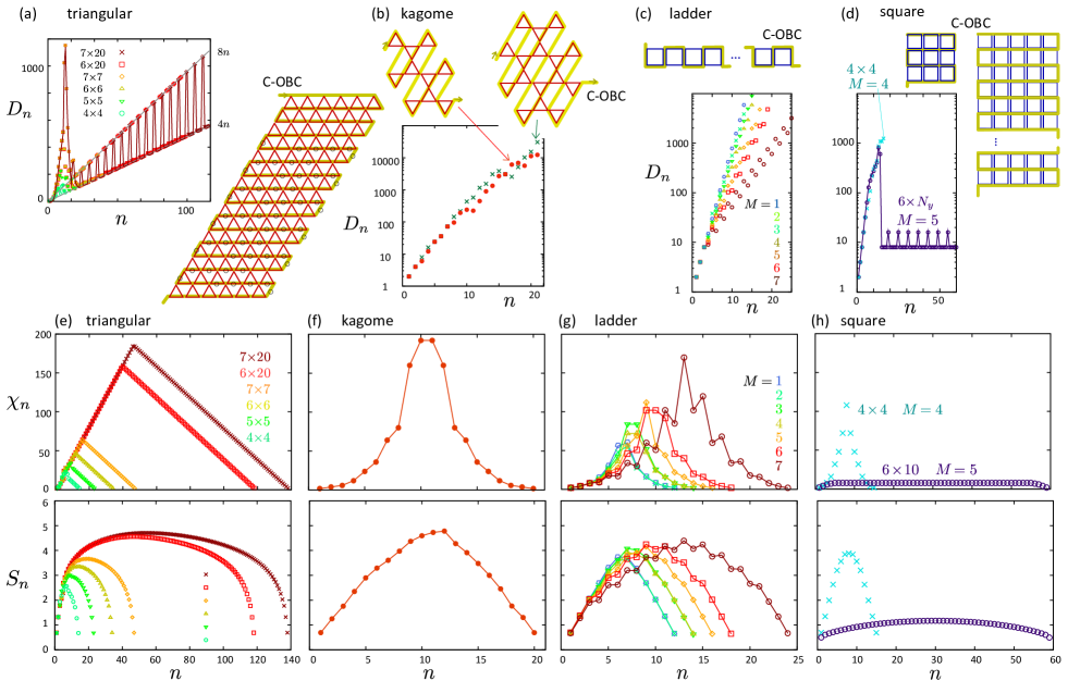
Figure 8: (a,b) $D_{n}$ of the exact MPS solutions of triangular and kagome lattice constructed using $n_{c}=3$ and $n_{\cap}=1$ for several choices of $N_{x}\times N_{y}$ with C-OBC. The left panel in (a) is the case of $N_{x}=7$, where for $7\times 20$ system, we find $D_{n}=4n$ for the bonds marked with a circle. (c,d) Ladder and square lattice with $n_{c}=4$, $n_{\cap}=2$, C-OBC, where we change the number of sites $M$ to be projected to see how $D_{n}$ grows. (e-h) Bond dimension $\chi_{n}$ after truncating the MPS and EE, $S_{n}$ as functions of bipartition size $n$. The data are averaged over $D_{N}$ ground states (see panels (a-d)), while for the kagome lattice, we choose 500 ground states among $D_{N}=12288$ to save the computational cost which does not alter the quality of the result.

IV.3 Variants of lattices for 2D MPS

We now apply the method to several lattices to demonstrate the available size and constructions of the spin-1/2 lattice models, where we consider the case of $M=2$, $D_{g}=6$ unless otherwise noted.

triangular lattice with C-OBC.  In Fig. 8(a) we show $n_{c}=3,n_{\cap}=1$ triangular lattice with C-OBC, where we plot $D_{n}$ as a function of $n$ for the MPS path taken along the yellow line in the snaky shape. For $7\times 20$ cluster with $N=139$ we find $D_{N}=560$ degenerate ground states. When $n<N_{y}$, we do not perform a projection so that the bond dimension grows in powers as $2^{n}$, while at larger $n$ we find that $D_{n}$ oscillates between fours successive $4n$’s and two $8n$’s, where the former bonds are marked by a circle in the figure.

kagome lattice with C-OBC.  We apply the same treatment for the kagome lattice as in Fig. 8(b). Because the number of triangles that require a projection is much less than the triangular lattice, $D_{n}$ grows exponentially with $n$, which means that it is practically difficult to deal with this lattice.

Ladder and square lattices with C-OBC.  We now examine other types of unit clusters, $n_{c}=4$, $n_{\cap}=2$ in a spin-1/2 model. Here, we increase the number of sites to be projected out from $M=1$ to $7$ in the following order,

$$|\xi_{1}\rangle=|0001\rangle+|0010\rangle+|0100\rangle+|1000\rangle,$$

$$|\xi_{2}\rangle=|1110\rangle+|1101\rangle+|1011\rangle+|0111\rangle,$$

$$|\xi_{3}\rangle=|0000\rangle,$$

$$|\xi_{4}\rangle=|1111\rangle,$$

$$|\xi_{5}\rangle=|0011\rangle+|0110\rangle+|1100\rangle+|1001\rangle,$$

$$|\xi_{6}\rangle=|0101\rangle+|1010\rangle,$$

$$|\xi_{7}\rangle=|0001\rangle-|0010\rangle+|0100\rangle-|1000\rangle,$$

$$|\xi_{8}\rangle=|1110\rangle-|1101\rangle+|1011\rangle-|0111\rangle.$$ (28)

Figure 8(c) shows $D_{n}$ for $M=1,\cdots,7$, finding that the exponential increase at $M\leq 6$ is suppressed and when $M=8$ we are able to construct the exact ground state up to $10\times 20$ lattice sites by suppressing the bond dimension to $D_{n}\leq 800$. However, for the square lattice, the number of projections increases; In Fig. 8(d) we show the case of $M=4$ at $5\times 5$ and $M=4$ at $6\times N_{y}$, $N_{y}\sim 20$, where we find that $D_{n}$ is ssuppressed to $10$ and do not change much with $n$. At $M\geq 6$ the number of bases per square is too small to entangle the state, and we no longer find the exact solution.

Entanglement entropy.   To make a more systematic understanding of the ground states of the above-mentioned lattices, we plot in Figs. 8(e)-(h) the bond dimension $\chi_{n}$ and the EE $S_{n}$, averaged over orthogonalized $D_{N}$ exact solutions with C-OBC. Here, when $\chi_{n}$ increases linearly as in the triangular case, the EE behaves as $\propto\ln n$, and its numerical cost is comparable to the well-known gapless 1D systems that the exact MPS feasible even in 2D. as one can see in the case of the ladder with quasi-linear $\chi_{n}$ in panel (g). The $M=5$ square lattice rather shows an area-law-like behavior, that keeps $\chi_{n}$ constant over a wide range of the system. In contrast, the kagome lattice shows a volume law, $S_{n}\propto n$, that makes $\chi_{n}$ increase exponentially fast.

IV.4 Random systems

We finally discuss the case of the spatially nonuniform Hamiltonians.

Quenched bond randomness. Let us again consider the triangular unit cluster, $n_{c}=3$ of spin-1/2, where we may choose

$$|\xi_{\Uparrow,l}\rangle=c_{l,1}|101\rangle+c_{l,2}|011\rangle+c_{l,3}|110\rangle)$$

$$|\xi_{\Downarrow,l}\rangle=c_{l,1}|010\rangle+c_{l,2}|100\rangle+c_{l,3}|001\rangle),$$ (29)

where $\bm{c}_{l}=(c_{l,1},c_{l,2},c_{l,3})\in{\mathbb{R}}$ are random variables. As in $\alpha=\pi/2$ in Eq.(44), $\hat{h}_{l}(\bm{c}_{l})=|\xi_{\Uparrow,l}\rangle\langle\xi_{\Uparrow,l}|+|\xi_{\Downarrow,l}\rangle\langle\xi_{\Downarrow,l}|$, is the XXZ cluster Hamiltonian whose three bonds typically have different values of $j^{z}$ and $j^{\perp}$. Notice that if we take $\bm{c}_{l}\in{\mathbb{C}}$ while keeping the time-reversal symmetry, $\hat{h}_{l}(\bm{c}_{l})$ starts to have the anisotropic and nonsymmetric exchange coupling terms such as $S_{i}^{x}S_{j}^{y}$ (see Appendix A).

We now generate ${\bm{c}_{l}}$ to be a uniform random distribution at $[-1:1]$ and consider two types of triangular lattice using the construction $n_{\cap}=2$ and $1$, as shown in Figs. 9(a) and 9(b), respectively. The distribution of $J^{z}$ and $J^{\perp}$ for the two constructions are shown, both with a peak at zero. Unfortunately, when $n_{\cap}=2$ the system can host only trivial all-up and all-down state solutions with two-fold degeneracy at $N_{x},N_{y}\geq 3$. When $n_{\cap}=1$, the degeneracy of the exact ground states increases to $\sim 4N$, which can be a good reference for the random-bond XXZ model as a quantum version of the Edwards-Anderson modelEdwards and Anderson (1975) studied extensively in the context of classical spin glassBinder and Young (1986). Indeed, there is an increasing interest in trying to elucidate the quantum disordered phase Watanabe et al. (2014); Shimokawa et al. (2015); Liu et al. (2018); Wu et al. (2019) in relevance to materialsKimchi et al. (2018).

Quite remarkably, even if we vary the absolute values $|\bm{c}_{l}|>0$ arbitrarily while keeping its structure unchanged, the energy eigenstates of the triangles do not change so that the lattice ground state remains the same. However, the distribution of $J^{z}$ and $J^{\perp}$ change. We show in the lower panel of Fig. 9(b) the case where we normalize $|\bm{c}_{l}|=1$, which differs much from the unnormalized ones. The physical implication of the stability of the exact ground state is put forward for future studies.

Sine square deformation. We add one more example that the Hamiltonian is not spatially uniform but useful. Consider again a 1D zigzag chain as in §.V, while we let the magnitude of $\hat{h}_{l}$ depend on the location of interactions as

$${\cal H}_{\rm SSD}=\sum_{l=1}^{N_{c}}\hat{f}_{\rm SSD}(\bm{r}_{l})h_{l}(\bm{r}_{l}),$$

$$f_{\rm SSD}(\bm{r}_{l})=\frac{1}{2}\big{(}1+\cos(\frac{\pi r_{l}}{R})\big{)},$$ (30)

where $R$ is the radius of a circle with its origin at the center of the lattice and $\bm{r}_{l}$ is the positional vector of the $l$-th cluster. We use the envelope function $f_{\rm SSD}$ which gradually scales down the interaction strength from 1 at the center to 0 at the edges of the lattice as shown in Fig. 9(c). This treatment is called sine-square deformation (SSD)Gendiar et al. (2009). Solving ${\cal H}_{\rm SSD}$ gives the same ground state wave function as the case of PBC for the gapped systemHikihara and Nishino (2011); Katsura (2011); Maruyama et al. (2011). It is also found useful to reduce the finite size effect significantlyGendiar et al. (2011); Kawano and Hotta (2022), and the physical properties measured at the center mimic those of $N\rightarrow\infty$ already at $N\sim 20$ Hotta and Shibata (2012); Hotta et al. (2013). In the present framework, the deformation simply modifies the eigenvalues of $\hat{h}_{l}$ but since we set the lowest energy state to zero, the ground state solution does not change with this modification. Finding such solutions would help to further clarify the role of SSD.

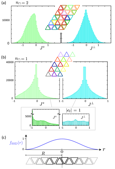
Figure 9: (a,b) Model with quenched randomness where $\hat{h}_{l}$ is determined by Eq.(29) depends on $l$. We set $n_{\cap}=2$ and $1$ where only the latter has a nontrivial ground state with $\sim 4N$ degeneracy. the distribution of $J^{z}$ and $J^{\perp}$ over $N_{x}=N_{y}=300$ bonds are shown. Lower panels are the distributions when we set $|\bm{c}_{l}|=1$ for all triangles. (c) Schematic illustration of the sine square deformation $f_{\rm SSD}(r)$ applied as envelope function of the lattice Hamiltonian to vary the amplitudes of $\hat{h}_{l}$ gradually over the system.

V Finding frustration-free models across the parameter space

So far we have focused on how to construct the exact MPS ground states from a given $\hat{h}_{l}$ (Case I). In this section, we demonstrate how to design a Hamiltonian (Case II) that can host the exact ground states by properly selecting $\{\xi^{m}\}$ and $\hat{h}_{l}$ in §.V.1,V.2 using the zigzag spin-1/2 chain as a platform. Then, we pay attention to the Hamiltonian we found in these results, and discover several extra exact solutions for these Hamiltonians in §.V.3.

V.1 Triangular unit

Let us consider a unit triangle consisting of three spin-1/2 shown in Fig. 10(a), whose up and down spins are denoted as $i_{n}=0,1$ and its $d^{n_{c}}=2^{3}$ basis states are given as $|i_{3}i_{2}i_{1}\rangle=|000\rangle,|001\rangle,\cdots$. In a zero magnetic field, the system naturally requires a time-reversal symmetry, and from among four time-reversal pairs we choose a single pair to be projected out as

$$|\xi_{\Uparrow}\rangle = \cos\alpha|000\rangle+i\sin\alpha\big{[}\cos\beta|101\rangle$$

$$\rule{34.1433pt}{0.0pt}+\sin\beta\big{(}\cos\delta|110\rangle+\sin\delta|011\rangle\big{)}\big{]}$$

$$|\xi_{\Downarrow}\rangle = \cos\alpha|111\rangle-i\sin\alpha\big{[}\cos\beta|010\rangle$$ (31)

$$\rule{34.1433pt}{0.0pt}+\sin\beta\big{(}\cos\delta|001\rangle+\sin\delta|100\rangle\big{)}\big{]},$$

which are parameterized by $0\leq\alpha,\beta,\delta\leq\pi$, encompassing all possible realizations for the combination of the four basis states for the bond-symmetric interactions. To include the antisymmetric Dzyaloshinskii-Moriya terms Moriya (1960), we need to extend the parameter to complex variables which we present in Appendix A. In §.V, unless otherwise noted, we focus on the case of $\delta=\pi/4$ that preserves the mirror symmetry of the triangle.

The local Hamiltonian is given as

$$\hat{h}_{l} =|\xi_{\Uparrow}\rangle\langle\xi_{\Uparrow}|+|\xi_{\Downarrow}\rangle\langle\xi_{\Downarrow}|$$

$$=\!\sum_{\eta}\!\big{(}j_{\eta}^{\perp}(S^{x}_{i}S^{x}_{j}+S^{y}_{i}S^{y}_{j})+j_{\eta}^{z}S^{z}_{i}S^{z}_{j}+\gamma_{\eta}(S^{x}_{i}S^{y}_{j}+S^{y}_{i}S^{x}_{j})\big{)}$$ (32)

where $\eta=1,1^{\prime},2$ denote the three bonds forming a triangle, and we denote $j_{\eta}^{z}/j_{\eta}^{\perp}=\Delta_{\eta}$ by convention. The exchange interactions are

$$j_{1}^{\perp} =\sin^{2}\alpha\sin 2\beta\sin\delta,$$

$$j_{1}^{z}\; =\cos^{2}\alpha-\sin^{2}\alpha(\cos^{2}\beta-\sin^{2}\beta\cos 2\delta),$$

$$\gamma_{1}\> =\sin 2\alpha\sin\beta\cos\delta,$$

$$j_{1^{\prime}}^{\perp} =\sin^{2}\alpha\sin 2\beta\sin\delta,$$

$$j_{1^{\prime}}^{z}\> =\cos^{2}\alpha-\sin^{2}\alpha(\cos^{2}\beta+\sin^{2}\beta\cos 2\delta),$$

$$\gamma_{1^{\prime}} =\sin 2\alpha\sin\beta\cos\delta,$$

$$j_{2}^{\perp} =\sin^{2}\alpha\sin^{2}\beta\sin 2\delta,$$

$$j_{2}^{z}\; =\cos^{2}\alpha+\sin^{2}\alpha\cos 2\beta,$$

$$\gamma_{2}\> =\sin 2\alpha\cos\beta.$$ (33)

When $\tan\beta=\sqrt{2}$ (i.e., $\cos\beta=1/\sqrt{3}$), the triangle is $C_{3}$ symmetric and we find $j_{1}=j_{1^{\prime}}=j_{2}$ and $\gamma_{1}=\gamma_{1^{\prime}}=\gamma_{2}$. The value of $\alpha$ controls the anisotropy of spins and when $\alpha=\pi/2$, we find an XXZ type of interaction, $\gamma_{\eta}=0$.

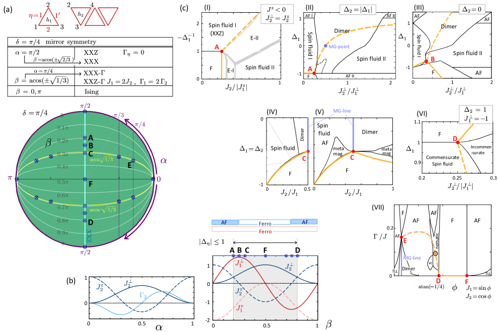
Figure 10: (a) Diagram of solution space at $\delta=\pi/4$ (mirror symmetry) on the plane of $\alpha,\beta=[0:\pi]$. (b) Model parameters of Eq.(34) along the XXZ line($\alpha=\pi/2$) $(J_{1}^{\perp},J_{1}^{z},J_{2}^{\perp},J_{2}^{z})=(\sqrt{2}\sin 2\beta,-2\cos^{2}\beta,\sin^{2}\beta,\cos 2\beta)$, and $J_{2}=2J_{1}$ line ($\cos\beta=\sqrt{1/3})$ with $(J_{2}^{\perp},J_{2}^{z},\Gamma_{2})=(2\sin^{2}\alpha/3,(2\cos 2\alpha+1)/3,\sin 2\alpha/\sqrt{3})$. (c) Phase diagrams of previous studies (I)F-AF XXZPlekhanov et al. (2010), (II)F/AF-AF XXZSomma and Aligia (2001), (III)FXXZ-XYJafari and Langari (2007), (IV,V)F-FXXZ Hirata and Nomura (2000); Gerhardt et al. (1998), (VI)F-AF XXXDmitriev and Krivnov (2008). (VII)XXX-$\Gamma$ modelsSaito and Hotta (2024a). Red bullets are the multicritical exact solutions with $M=2$ and Orange solid lines are the exact solutions with $M=4$ (broken lines are those that do not have solutions ($D_{N}=0$). The amplitudes of parameters are scaled together arbitrarily.

V.2 Exactly solvable diagrams of zigzag chain

We consider a zigzag chain obtained by consecutively linking $(123),(234),\cdots$ clusters.

$${\cal H}_{N} =\sum_{\eta=1,1^{\prime},2}\sum_{\langle i,j\rangle}\big{(}J_{\eta}^{\perp}(S^{x}_{i}S^{x}_{j}+S^{y}_{i}S^{y}_{j})+J_{\eta}^{z}S^{z}_{i}S^{z}_{j}$$

$$\rule{56.9055pt}{0.0pt}+\Gamma_{\eta}(S^{x}_{i}S^{y}_{j}+S^{y}_{i}S^{x}_{j})\big{)},$$ (34)

where interaction runs over neighboring pairs of spins $\langle i,j\rangle$, and $J_{1}^{\perp/z}=2j_{1}^{\perp/z}$, $J_{2}^{\perp/z}=j_{2}^{\perp/z}$, $\Gamma_{1}=2\gamma_{1}$, $\Gamma_{2}=\gamma_{2}$, because the diagonal bonds are doubled. When we leave the boundary of the cluster open, which we call cluster-open boundary, the boundary bonds are not doubled.

We first highlight the results obtained by this parameterization in Fig. 10(a). The “solution-space diagram” is depicted by setting $\alpha$ as polar radius and varying $\beta$ in the vertical axis for fixed $\alpha$. All the parameters on this plane have exact solutions. There are two distinct lines; the vertical $\alpha=\pi/2$ line represents the XXZ model with $\Gamma_{\eta}=0$, and along the horizontal $\beta={\rm acos}(\pm\sqrt{1/3})$, all the diagonal rung bonds $\eta=1$ have twice as large amplitudes of interactions as those of the legs $\eta=2$ (see Fig. 10(a)). The representative points with high-symmetry model parameters are summarized in Table I.

V.2.1 Spatially anisotropic XXZ models

Let us first focus on the XXZ models ($\alpha=\pi/2$, see Table I(a) and Fig. 10(a)); The $\beta=0,\pi$ limits are the AF Ising chains coupled by the F zigzag bonds, which has a trivial ground state. When $\cos\beta=\pm\sqrt{2/3}$ (A and D) the spin SU(2) symmetry is recovered and we find an F-AF zigzag Heisenberg (XXX) model.

The values of coupling constants as functions of $\beta$ are shown in the right panel of Fig. 10(b). The zigzag interaction is ferromagnetic ($J_{1}^{z}<0$), while both the F and AF leg interactions $J_{2}^{z}$ are realized. We find $|\Delta_{\eta}|\leq 1$ between A and D. A wide range of magnetic anisotropy for an F/AF-F XXZ chain has room to afford exactly solvable ground states.

Table 2: Representative parameters $\alpha,\beta$ at $\delta=\pi/4$ plane with mirror symmetry. (a) $\cos\alpha=0$ ($\alpha=\pi/2$) line having $\Gamma_{\eta}=0$ and (b) $\cos\beta=\pm\!\sqrt{1/3}$ line with $J_{1}^{\perp/z}=\pm 2J_{2}^{\perp/z}$ and $\Gamma_{2}=2|\Gamma_{1}|$. These points have high symmetry in their model parameters, where XXX and I represent the Heisenberg and Ising model, XY the case with $J_{\eta}^{z}=0\>(\Delta_{\eta}=0)$. Points A-F refer to the ones that appear in Fig. 10.

(a) XXZ line	$\cos\alpha=0$, $\delta=\pi/4$
	$\cos\beta\;$	$(\>J_{1}^{\perp},\;\;J_{2}^{\perp},\;\;J_{1}^{z},\;\;J_{2}^{z}\;\;)$
F-AF I	$\pm 1\>$	$(\;\;0,\;\;\;\;0,\;\;\;\;-2,\;\;1\;\;)$
F-AF XXX	$\sqrt{2/3}\>$	$(\>4/3,\;1/3,-4/3,\;\>1/3\>)$		A
F-AF XXX	$-\sqrt{2/3}\;$	$\!(-4/3,\;1/3,-4/3,\;\>1/3\>)$		D
F-F XXZ	$\sqrt{1/3}\;$	$(\>4/3,\;2/3,-2/3,-\!1/3\>)$		C
FXXZ-XY	$\sqrt{1/2}\;$	$(\>\sqrt{2},\;1/2,\!-\sqrt{1/2},\;\;\;\;0\;\;)$		B
FXXX(decoupled)	0	$(\;\;0,\;\;\;\;1,\;\;\;\;0,\;\;-1\;\;)$		F
(b) $J_{1}=2J_{2}$ line	$\cos\beta=\!\sqrt{1/3}$, $\delta=\pi/4$
	$\cos\alpha$	$(\;\;J_{2}^{\perp},\;\;J_{2}^{z},\;\;\;\Gamma_{2}\;\;)$
F-F XXZ	0	$(\;2/3,\;\;-\!1/3,\;\;\;0\;\;)$
XY$\Gamma$	$\pm 1/2$	$(\;1/2,\;\;\;\;\;0,\;\;\pm 1/2\;)$
AF XXX-$\Gamma$	$\pm\!\sqrt{1/2}$	$(\;1/3,\>\;1/3,\pm\sqrt{1/3}\;)$		E
AF I	$\pm 1\;$	$\;(\;\;0,\;\;\;\;\;1,\;\;\;\;0\;\;)$

The present framework successively connects different exact solutions that appear in different models that are separately studied in previous literature. The six phase diagrams that host A to D states are summarized in Fig. 10(c) (I)-(VI)Plekhanov et al. (2010); Somma and Aligia (2001); Jafari and Langari (2007); Hirata and Nomura (2000); Gerhardt et al. (1998); Dmitriev and Krivnov (2008); Saito and Hotta (2024a), which are variants of F-AF XXZ models. Here, we refer to F or AF interactions as those of $J_{\eta}^{z}$, because the local unitary transformation rotating the spin quantization axis on either of the legs by $\pi$ converts $J_{1}^{\perp}\rightarrow-J_{1}^{\perp}$, but does not change the physical states. It is widely accepted that in a series of materials consisting of edge-shared CuO₂ chains such as Rb₂Cu₂Mo₃O₁₂Hase et al. (2004), Na₂Cu₂O₂Drechsler et al. (2005), and LiCuVO₄Enderle et al. (2005) are represented by the F-AF XXZ models.

In the phase diagram Fig. 10(c)-(I) taken from the DMRG study in Ref.[Plekhanov et al., 2010], two gapless spin fluid phases are observed, having a zigzag and strong-leg characters, respectively. The ferromagnetic (F), spin fluid I, and the other two phases with massive excitations merge at the single point A, which forms a multicritical point. This point is exactly solved in our framework.

Analogous XXZ-types of models that interpolate F ($\Delta_{1}=-1$) and AF($\Delta_{1}=1)$ zigzag interactions in Figs. 10(c)-(II)Somma and Aligia (2001) and (III)Jafari and Langari (2007) exhibit essentially similar diagrams, insensitive to $\Delta_{2}$. At $J_{2}^{\perp}/J_{1}^{\perp}\gtrsim 0.5$, one finds a gapped dimer singlet phase, sandwiched by Spin fluid I and II. When $|\Delta_{\eta}|\geq 1$ the system becomes massive and develops either F or AF long-range orders.

It is noteworthy that in diagram (III), Ref.[Jafari and Langari, 2007] did not detect the multicritcal point B located at $(J_{2}^{\perp}/J_{1}^{\perp},\Delta_{1})=(\sqrt{1/8},-\sqrt{1/2})$. This manifests that for model parameters with an irregular anisotropy, it is difficult to predict or confirm numerically whether several phases exactly meet at a single point.

Similarly, in the AF-AF SU(2) Heisenberg case (diagrams (IV, V)), there is another point C with $J_{2}/J_{1}=0.5$, $\Delta_{1}=\Delta_{2}=-1/2$ at which the F and Dimer phases meet. As we see shortly, it is the endpoint of the Majumdar-Ghosh line, hosting an exact dimer singlet-product ground stateMajumdar and Ghosh (1969a, b). The phase diagram in panel (V)Gerhardt et al. (1998) was studied in search of metamagnetic phase, which shows a magnetization jump in an applied magnetic field as observed in several materials like Fe_xMn_1-xTiO₃, GdNi₂Sb₂ and GdCu₂Sb₂ Ito et al. (1992); Lelievre-Berna et al. (1993); Kaczmarska et al. (1995). Indeed, C is a multicritical point where the metamagnet merges with dimer and F phases.

The multicritical point D in the phase diagram (VI) has further interesting property; it has both the $S=0$ ground state and fully polarized $S=N/2$ ferromagnet to be perfectly degenerate, and the former is not the Majumdar-Ghosh product state but another highly entangled state called uniformly distributed resonating valence bond state (UDRVB). Hamada, et.al. discovered a UDRVB as an exact ground state at $J_{2}=-J_{1}/4$, $(J_{1}<0)$ (this F-AF model is called the generalized railroad trestle model)Hamada et al. (1988).

V.2.2 $J_{1}=2J_{2}$ $\Gamma$ model

At $\alpha\neq\pi/2$, the finite $\Gamma_{\eta}$-terms appear. We particularly focus on the $\cos\beta=\sqrt{1/3}$ line where the $C_{3}$ symmetry of the unit triangle leads to twice as large zigzag coupling against the leg couplings, $J^{\perp/z}_{1}=2J_{2}^{\perp/z}$ and $\Gamma_{1}=2\Gamma_{2}$. When we further take $\cos\alpha=\sqrt{1/2}$ the AF Heisenberg coupling, $J^{\perp}_{\eta}=J^{z}_{\eta}\equiv J_{\eta}$ is realized at E. It appears as a multicritical point of the phase diagram of the Heisenberg $J_{1}$-$J_{2}$ model with finite $\Gamma$ term shown in Fig. 10(c)-(VII)Saito and Hotta (2024b). Here, we plot it on the plane of $\Gamma_{\eta}/J_{\eta}$ and $\phi={\rm atan}(J_{2}/J_{1})$ with $J_{2}=\cos\phi$ and $J_{1}=\sin\phi$. The multicritical point E has $J_{1}=2J_{2}$ and $\Gamma_{\eta}=\sqrt{3}J_{\eta}$, where five phases meet, and similarly to point C it is part of the Majumdar-Ghosh line that extends from $\Gamma_{\eta}=0$. Our method interpolates point E with the other two points, D and F within the same $\delta=\pi/4$ (Fig. 10(a)). Point D hosting RVB appears at $\phi={\rm atan}(-1/4)$ where the RVB with $S=0$ and the fully polarized ferromagnetic solution $S=N/2$ coexist. The latter extends to larger $\phi$ toward the endpoint F, at which we find a decoupled ferromagnetic Heisenberg chain.

V.3 Exact solution lines in the phase diagrams

So far we have designed the form of the Hamiltonian following Case II in §.II.1 that elucidates the bulk exact solutions. These solutions appears as “isolated points”, A-F, in the phase diagrams of Fig. 10(c). However, if we focus on a given Hamiltonian in each diagram and vary the model parameters, we find that these points are not isolated but are connected to the exact solution lines.

To find such lines, we diagonalize the unit cluster Hamiltonian $\hat{h}_{l}$, and see how the degeneracy $D_{g}$ of the lowest energy manifold changes with model parameters, which we referred to as Case I. In §.V.1 we considered $D_{g}=6$ ($M=2$) for multi degenerate solutions at A-F, which are the tricritical(multicritical) points at which three phase boundaries meet. In addition, $\hat{h}_{l}$ can have $D_{g}=4$ ($M=4$) along the bold lines of Fig. 10(c)(I)-(VII). Among them, the solid lines have the bulk exact solution, which include the Majumdar-Ghosh lines or points, a well-known singlet-product ground state of the zigzag chain. It is noteworthy that these exactly solved lines very often coincide with the numerically obtained phase boundary, e.g. in Fig. 10(c)-(IV),(V), at which F and spin fluid phases meet. The broken lines do not have such solutions but connect different multicritical points. Indeed, in Fig. 10(c)-(VII), we newly find an exact nematic product solution on the broken line inside the nematic phase. This broken line connects the two multicritical points, E and D. These results show that the present framework is useful to clarify the ground state phase diagram with a very small numerical cost of diagonalizing the small unit cluster. It reminds us of a level spectroscopy analysis that successfully detects the phase boundary using exact diagonalizationNomura and Okamoto (1994); Kitazawa (1997).

We notice that these exact ground state solutions discussed here in Fig. 10 are gapless for the corresponding frustration-free Hamiltonian. Indeed, the ones found along the XXZ lines are equivalent to the one previously reported as gapless based on the exact analysis using anyonsBatista (2009).

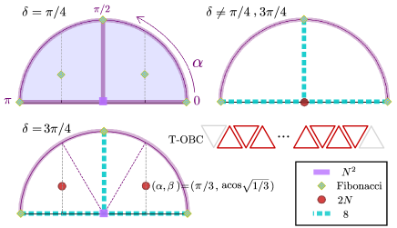
Figure 11: Solution space of the zigzag spin-1/2 chain based on a triangular unit with the choice of $M=6$ in Eq.(31), where $\alpha$ is the tangent and $\beta$ denotes the vertical line as in Fig. 10(a). For all cases, $\beta=[\pi/2:\pi]$ range has the same types of solution as the ones with $\beta=[0:\pi/2]$ and is abbreviated. The range without any symbols or lines has no exact solution. $\delta=\pi/4,3\pi/4$ and off these two are shown in different panels.

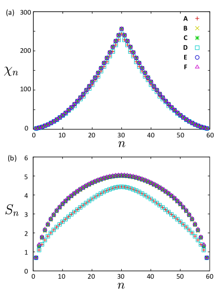
Figure 12: (a) Bond dimension $\chi_{n}$ and (b) EE $S_{n}$ of the exact MPS solutions of the zigzag spin-1/2 chain with $N=60$ C-OBC, obtained at parameters A-F in Fig. 10(a). The results are averaged over the orthogonalized $D_{N}$-degenerate solutions.

V.4 Classification of the exact solutions

V.4.1 Degeneracy

There are two important pieces of information in addition to the phase diagram; whether we have a set of Hamiltonian and exact solution or not for a given parameter, and if yes, how the degeneracy grows with $N$, which provides us with the nature of the obtained ground state.

We focus on a wider range of parameters than we did in the previous subsection and show the “solution diagram” with information about the types of degeneracy in Fig. 11(a)-11(c) for $\delta=\pi/4,3\pi/4$ and otherwise. Here, we consider the zigzag chain with cluster open boundary (C-OBC), where we leave the edge triangles not to link to the other edges. We can add a unit triangle one by one to evaluate $D_{N}^{{\rm TOBC}}$ by rank$Q$ iteratively. There are four types of degeneracy: $D_{N}$ increasing with order-$N^{2}$, with Fibonacci sequence, with $2N$, and constant $D_{N}=8$. Here, notice that by definition in Eq.(31) once we take $\alpha=0,\pi$ the other two parameters $\beta,\delta$ do not make sense, and so as $\beta=0,\pi$ about $\delta$.

$N^{2}$-type degeneracy: The degeneracy increasing in a square appears in almost the whole region of the diagram at $\delta=\pi/4$ except for a few points. In increasing the number of triangles linked and obtaining the form of $Q$, we find an iterative relationship, ${\rm dim}(\cap_{l=1}^{n}V_{l})/{\rm dim}(\cap_{l=1}^{n-1}V_{l})=(n+4)(2(n+2))$ for odd-$n$ and $(n+5)(2(n+3))$ for even-$n$ with $n\leq N_{c}=N-2$ for C-OBC. Accordingly, we obtain the exact form,

$$D_{N}^{{\rm TOBC}}=\left\{\begin{array}[]{ll}(N+2)^{2}/4&({\rm even}\;\;N)\\ (N+1)(N+3)/4&({\rm odd}\;\;N).\end{array}\right.$$ (37)

The degeneracy increasing in powers implies that the system is possibly gapless and is found to be a specific multicritical point, which is observed previously in some specific model parametersBatista (2009); Batista and Somma (2012); Changlani et al. (2018); Palle and Benton (2021). In the standard critical phase in quantum many-body systems, the ground state of a finite-size system is unique and has a finite-size gap that closes with $N^{-1}$ or $N^{-2}$Cardy (1996). However, when more than two phases meet at multicritical points, highly degenerate states can appear as ground states As in Fig. 10 (c)-(III) B, the multicritical point moves away from the highly symmetric model parameters when we vary $\alpha$ and $\beta$, and our solution can track them.

Fibonacci-sequence: Interestingly, degeneracy can sometimes form a Fibonacci sequence with increasing $N$ as $2,2,4,6,10,16\cdots$, namely

$$D_{N}^{{\rm TOBC}}=2F_{N},$$ (38)

where $F_{N+2}=F_{N+1}+F_{N}$. These points appear at eight isolated points, $\alpha=0,\pi$, $(\alpha,\beta)=(\pi/2,0),(\pi/2,\pi)$, and $(\alpha,\beta)=(\pm\pi/3,{\rm acos}(\pm\sqrt{1/3}))$ with $\delta=\pi/4$. This degeneracy is an Ising-typeRedner (1981), and increases exponentially with $N$.

$2N$-type: Solutions with degeneracy increasing linearly as $D_{N}=2N$ appear along the lines of the $\alpha\beta$-plane as $\alpha=\pi/2$ and $\beta=\pi/2$ for all values of $\delta$.

Constant-type: At $\alpha=\pi/2$ or $\beta=\pi/2$, the 8-fold degeneracy appears for $N\geq 4$.

V.4.2 Exact MPS solutions

One can obtain the MPS solutions for this zigzag spin-1/2 chain as well using the treatment given in §.III. Figure 12 shows the bond dimension $\chi_{n}$ and EE $S_{n}$ for $N=60$ C-OBC solutions obtained for the parameters A-F. One finds that $\chi_{n}$ after truncated is basically equivalent to $D_{n}$ up to $n\leq N/2$ that follows Eq.(37), and the EE follows $S_{n}\propto\ln n$.

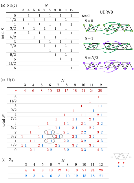
Figure 13: Distribution of degeneracy of $N^{2}$-type ground states of the zigzag chain with C-OBC classified according to the conservation number. (a) Heisenberg model with SU(2) symmetry realized at $\beta={\rm acos}(-\sqrt{2/3})$ at point D. A schematic illustration of the RVB state is shown on the right panel where a pair of sites connected by arrows denotes the singlet, and a pair connected by a broken line is the triplet. (b) XXZ model ($\alpha=\pi/2,\;\delta=\pi/4$) with U(1) symmetry, classified by the total $S^{z}$ where we show only the $S^{z}\geq 0$ part. (c) XYZ model at $\alpha\neq\pi/2$ having ${\mathbb{Z}}_{2}$ symmetry. The red and blue numbers in panels (b) and (c) are those that have $+1$ and $-1$ eigenvalues about the mirror operation against the vertical axis of the center of the cluster.

V.4.3 Symmetry and RVB state

As mentioned in §.II.2, the exact solutions for a given $N$ can be classified by the symmetries. Here, we focus on the $N^{2}$-type degeneracy solutions found at $\delta=\pi/4$ for a zigzag chain with C-OBC (see Figs. 10(a) and 11). The spins have SU(2) symmetry at A, D, F, U(1) symmetry at other points along the XXZ line, and ${\mathbb{Z}}_{2}$ the other parts of the $\alpha$-$\beta$ plane except for a few points.

To understand the origin of degeneracy, it is useful to classify the solutions according to the conservation numbers. This is done by projecting the ground state solutions to the corresponding subspace. In Figs. 13(a)-(c) we show how the numbers of solutions distribute for a given $N$, where total $S$ and total $S^{z}$ are used for SU(2) and U(1) cases, respectively. Here, we classify the U(1) and ${\mathbb{Z}}_{2}$ cases further by whether they have $\pm 1$ eigenvalues about the mirror operation against the plane perpendicular to the zigzag ladder. The degeneracy at $(N,S^{z})$ is related to either of larger ones at $(N-1,S^{z}\pm 1/2)$. Although the conservation numbers change, they shall be related.

We now show that the present analysis helps us clarify the nature of the RVB state at point D. The exact solution is called RVB given in the formHamada et al. (1988),

$$|\Phi_{\rm RVB}\rangle=\sum_{i_{1}<j_{1},i_{2}<j_{2},\cdots}[i_{1},j_{1}][i_{2},j_{2}]\cdots,$$

$$\quad[i,j]=(|01\rangle-|10\rangle)/\sqrt{2},$$ (39)

where the summation is taken over all possible combinations of pairs of sites with no duplication on site indices. Here, $[i,j]$ is the singlet formed on $i,j$-th pair of sites, written as arrows in Fig. 13(b). It was shown thatHamada et al. (1988) the $S=0$ RVB is degenerate with the $S=N/2$ fully polarized state for PBC because this parameter is at the boundary of the two phases (see Fig. 10(c)-(VI)). A new finding here is that in C-OBC, all the spin sectors (that were the excited states in PBC) become degenerate with $S=0,N/2$ and join the ground state; we find that the number of degeneracy in Eq.(37) comes from the number of all different total-$S^{z}$ and total-$S$ sectors given in Fig. 13(b). Using our MPS solution (see §.III.1), we discover the exact form of the $S=1$ state: it is obtained by replacing the first singlet $[i,j]$ to triplet $(i,j)$ as

$$|\Phi_{S=1}\rangle=\sum_{i_{1}<j_{1},i_{2}<j_{2},\cdots}(i_{1},j_{1})[i_{2},j_{2}],[i_{3},j_{3}]\cdots.$$ (40)

In the same manner, the $S=m$ state has the form of replacing the first $m$ successive singlet in Eq.(39) to triplet as well. The reason why the states $S\neq 0,N/2$ become the excited state for PBC is that they cannot fulfill the translational invariance. It is natural to expect all of them to collapse to the ground state at $N\rightarrow\infty$, providing us with the state beyond the simple RVB.

VI summary and discussion

We have proposed a framework to concurrently design a lattice Hamiltonian and determine an exact ground state in quantum many-body systems belonging to the class of frustration-free models. This framework addresses the challenge of going over the limit of accurately approximating unbiased ground states, which goes across both the gapped and gapless, short-entangled to long-range entangled states, particularly in large-scale systems where computational costs escalate significantly.

We begin by introducing a unit cluster and categorizing states into two distinct manifolds: one contributing to the ground state and the other not, belonging to the lowest energy level and excited levels of the cluster Hamiltonian, respectively. The lattice Hamiltonian is formulated as a sum of local cluster Hamiltonians with overlapping clusters. By zeroing out the excited manifold of the cluster state, the lowest-energy manifold enters the full many-body lattice wave function.

It is then imperative to entangle the lowest energy states among different clusters. The key to our framework projects the Hilbert space onto these states over all clusters, ensuring an unbiased ground state determination that can be systematically applied across various models. When further employing the matrix product state approach, we can progressively expand the system size and iteratively apply the projection to newly added clusters to determine their matrices. We can take full advantage of the techniques developed for matrix product states like canonical form or truncation. Given the precise knowledge that the ground state energy is set to zero and the positive semidefiniteness of the Hamiltonian, validating exact solutions is straightforward.

One can systematically search for such Hamiltonians by parameterizing the lowest energy cluster states as linear combinations of chosen basis states. This approach offers various types of models and facilitates connections between different exact solutions found in various contexts. We provide a demonstration using the spin-1/2 zigzag chain, showcasing exact ground states whose degeneracy increases quadratically with the system size, revealing connections between previously reported phase diagrams in anisotropic XXZ-type models. As a novel discovery, we found that the resonating valence bond (RVB) state of the ferro-antiferro zigzag chain model previously reported by Hamada et. al. Hamada et al. (1988) exhibits additional macroscopic degeneracy across all total $S$-sectors. This implies the condensation of all allowed numbers of magnons, suggesting a multi-magnon Bose-Einstein condensate atop the RVB sea.

Related work by Batista et al. Batista (2009); Batista and Somma (2012) has found an exact solution for the antiferromagnetic XXZ model on the zigzag ladder, exhibiting the same degeneracy as shown in Eq.(37). They employed a generalized Jordan-Wigner transformation to map spins to anyons and identified a BEC ground state of anyons carrying momentum $Q$, represented as $(a_{Q})^{n}(a_{-Q})^{m}|0\rangle$, where the choice of adding $n$ and $m$ anyons explains the origin of the degeneracy. It corresponds to the XXZ line of our zigzag chain at $\alpha=\pi/4$ with total $S^{z}=n+m-N/2$. They also derived the specific form of the matrix product state (MPS) solution for $Q=2\pi/p$ of bond dimension $p-1$. However, there is no one-to-one correspondence between their periodic MPS representation and ours, as the MPS representation has large facultativity. While their approach may apply to models with specific conservation numbers or geometries, such cases are not easily identified. Our method helps to relate these results with other models as we did in Fig. 10.

We also demonstrated the application to 2D systems that exhibit comparable computational costs to the 1D case. However, in 2D, the bond dimensions can grow more rapidly than 1D, especially when the overlap of neighboring clusters is small as $n_{\cap}=1$. Notably, on the kagome lattice, the degeneracy undergoes exponential growth, but decreasing $D_{g}$ leads to over-suppression of the state entanglement. Nonetheless, intriguing states with exact matrix product state (MPS) solutions of moderate bond dimensions exist. Previously, spin-1/2 model on the kagome lattice at specific interaction strength, $J^{z}/J^{\perp}=-1/2$, called XXZ0, was known to exhibit three-coloring product stateChanglani et al. (2018), detected via exact diagonalization(ED). It features macroscopic degeneracy attributed to classical frustration effects as three-coloring patterns discussed previously in the classical kagome modelsHarris et al. (1992); Chalker et al. (1992); Henley (2009). However, for larger system sizes, numerous other degenerate ground states exist that defy such simple product state explanations. The XYZ model also showcases three-coloring degenerate ground states using different basis setsPalle and Benton (2021). Although these three-colored states apply to various lattice geometries, such as sawtooth, zigzag, and triangular, they possess essentially unique three-coloring patterns and fail to elucidate the highly entangled underlying states demonstrated in our study.

These prior works have partially introduced the concept of utilizing cluster states to derive a bulk ground state in a so-called frustration-free Hamiltonian given by the positive definite operators Changlani et al. (2018); Palle and Benton (2021); Batista and Somma (2012); Alexander et al. (2021). However, their methodology relies on conserved quantum numbers for construction, wherein they define a vacuum state and introduce fictitious free particles capable of condensation. These states thus obtained are product states, similarly to Majumdar-Ghosh singlet-product stateMajumdar and Ghosh (1969a, b) and its generalization to 2D frustrated latticesKlein (1982); Ghosh et al. (2022); Miyahara and Ueda (1999). Another series of exact solutions in quantum many-body systems are the long-range entangled states hosted by Kitaev and toric code models Kitaev (2003, 2006), and several toy models sharing similar structures were developed which proved useful to elucidate the nature of such liquid statesWen (2003); Wang et al. (2017). As mentioned in the introduction and in §.II.1, there are also series of works on injective MPS having a translationally invariant formPerez-Garcia et al. (2007); Cirac et al. (2021), where it is mathematically proven that for any given injective MPS one can find a frustration-free parent Hamiltonian. However, these descriptions are limited to the gapped unique ground states. Our MPS that allows for far more degrees of freedom by imposing minimal conditions on the MPS are shown to describe both the gapless ground states, e.g. A-E in the zigzag spin 1/2-chain, and the topologically ordered ground states of the toric code, particularly allowing for the determination of a set of exact ground states of all topological sectors. We briefly mention that the area-law expected for MPS is not going to limit the representation of the finite-$N$ quantum many-body states even at finite temperature both in 1D and 2D known to have a volume lawIwaki et al. (2021); Gohlke et al. (2023), consistent with the present findings.

Our protocol for generating matrix product states proves valuable for systems outside these particular regimes empirically known. Indeed, physically meaningful models for laboratory studies often necessitate maintaining the natural and standard form of the Hamiltonian, which makes the quantum state intriguing. Importantly, our approach achieves finding some particular points to be exactly solved in a class of frustration-free models, without the need for additional numerical approximations or prior knowledge.

Exact solutions obtained on a large scale provide rigid theoretical starting points for exploring unknown quantum many-body phases. The spin liquid phase of a regular Heisenberg kagome antiferromagnet is discussed about three-coloring solutionsCépas and Ralko (2011); Changlani et al. (2018), and the quantum scar states that get rid of thermalization can be studied by obtaining exact scar tower of states in the integer-spin 1D AKLT is Moudgalya et al. (2018); Mark et al. (2020). The present framework can provide a platform for many such models and helps to clarify the underlying complexity of quantum many-body states.

Appendix A Cluster Hamiltonian of a triangle with antisymmetric exchange term

Here, we extend the parameter space of the choice of the cluster states from the ones shown in Eq.(31). We include the parameters $\lambda,\mu,\nu$ to have the complex number of coefficients as

$$|\xi_{\Uparrow}\rangle = e^{i\lambda}\cos\alpha|000\rangle+i\sin\alpha\big{[}e^{i\mu}\cos\beta|101\rangle$$

$$\rule{8.53581pt}{0.0pt}+\sin\beta\big{(}e^{i\nu}\cos\delta|110\rangle+\sin\delta|011\rangle\big{)}\big{]},$$

$$|\xi_{\Downarrow}\rangle = e^{-i\lambda}\cos\alpha|111\rangle-i\sin\alpha\big{[}e^{-i\mu}\cos\beta|010\rangle$$ (41)

$$\rule{8.53581pt}{0.0pt}+\sin\beta\big{(}e^{-i\nu}\cos\delta|001\rangle+\sin\delta|100\rangle\big{)}\big{]},$$

Here, when we apply a local gauge transformation $U_{z}(\theta)=e^{-i\sigma_{z}\theta/2}$ to rotate the spin $xy$-axis by $\theta$ about the $z$-axis, which transforms the up and down spin states as $|0\rangle\rightarrow e^{-i\theta/2}|0\rangle$ and $|1\rangle\rightarrow e^{i\theta/2}|1\rangle$, we find

$$\hat{h}_{l}(\alpha,\beta,\delta,\lambda,\mu,\nu)\rightarrow\hat{h}_{l}(\alpha,\beta,\delta,\lambda-2\theta,\mu,\nu),$$ (42)

which does not change the property of the Hamiltonian. Therefore, we set $\lambda=0$ and focus on the other two parameters. The resultant coupling constants include several terms that are not considered in the main text as

$$\hat{h}_{l}=\sum_{\langle i,k\rangle=1,1^{\prime},2}\sum_{\eta,\zeta=x,y,z}j_{ik}^{\eta\zeta}S_{i}^{\eta}S_{k}^{\zeta}$$ (43)

with the exchange couplings for $\langle i,k\rangle=\langle 1,2\rangle$, $\langle 2,3\rangle$, and $\langle 1,3\rangle$ indexed as 1,1’, and 2, respectively. They are given as

$$j_{1}^{xx} =j_{1}^{yy}=\sin^{2}\alpha\sin 2\beta\cos\delta\cos(\nu-\mu),$$

$$j_{1}^{xy} =\sin^{2}\alpha\sin 2\beta\cos\delta\cos(\nu-\mu)+\sin 2\alpha\sin\beta\sin\delta,$$

$$j_{1}^{yx} =-\sin^{2}\alpha\sin 2\beta\cos\delta\cos(\nu-\mu)+\sin 2\alpha\sin\beta\sin\delta,$$

$$j_{1}^{zz}\; =\cos^{2}\alpha+\sin^{2}\alpha(-\cos^{2}\beta+\sin^{2}\beta\sin^{2}\delta),$$

$$j_{1^{\prime}}^{xx} =\sin^{2}\alpha\sin 2\beta\sin\delta\cos\mu-\sin 2\alpha\sin\beta\cos\delta\sin\nu,$$

$$j_{1^{\prime}}^{yy} =\sin^{2}\alpha\sin 2\beta\sin\delta\cos\mu+\sin 2\alpha\sin\beta\cos\delta\sin\nu,$$

$$j_{1^{\prime}}^{xy} =\sin^{2}\alpha\sin 2\beta\sin\delta\sin\mu+\sin 2\alpha\sin\beta\cos\delta\cos\nu,$$

$$j_{1^{\prime}}^{yx} =-\sin^{2}\alpha\sin 2\beta\sin\delta\sin\mu+\sin 2\alpha\sin\beta\cos\delta\cos\nu,$$

$$j_{1^{\prime}}^{zz}\; =\cos^{2}\alpha+\sin^{2}\alpha(-\cos^{2}\beta-\sin^{2}\beta\sin^{2}\delta),$$

$$j_{2}^{xx} =\sin^{2}\alpha\sin^{2}\beta\sin 2\delta\cos\nu-\sin 2\alpha\cos\beta\sin\mu,$$

$$j_{2}^{yy} =\sin^{2}\alpha\sin^{2}\beta\sin 2\delta\cos\nu+\sin 2\alpha\cos\beta\sin\mu,$$

$$j_{2}^{xy} =\sin^{2}\alpha\sin^{2}\beta\sin 2\delta\sin\nu+\sin 2\alpha\cos\beta\cos\mu,$$

$$j_{2}^{yx} =-\sin^{2}\alpha\sin^{2}\beta\sin 2\delta\sin\nu+\sin 2\alpha\cos\beta\cos\mu,$$

$$j_{2}^{z}\; =\cos^{2}\alpha+\sin^{2}\alpha\cos 2\beta.$$ (44)

In addition to the symmetric $\Gamma$-term that have equal $xy$ and $yx$ elements, the antisymmetric Dzyaloshinskii-Moriya interaction terms like $j^{xy}=-j^{yx}$ appear for this treatment. This will widely expand the model that provides the exact solution since the antisymmetric term ubiquitously appears in materials when the local bond inversion symmetry is lost.