A Compass for Navigating the World of Sentence Embeddings for the Telecom Domain

Abstract

A plethora of sentence embedding models makes it challenging to choose one, especially for domains such as telecom, rich with specialized vocabulary. We evaluate multiple embeddings obtained from publicly available models and their domain-adapted variants, on both point retrieval accuracies as well as their (95%) confidence intervals. We establish a systematic method to obtain thresholds for similarity scores for different embeddings. We observe that fine-tuning improves mean bootstrapped accuracies as well as tightens confidence intervals. The pre-training combined with fine-tuning makes confidence intervals even tighter. To understand these variations, we analyse and report significant correlations between the distributional overlap between top-$K$, correct and random sentence similarities with retrieval accuracies and similarity thresholds. Following current literature, we analyze if retrieval accuracy variations can be attributed to isotropy of embeddings. Our conclusions are that isotropy of embeddings (as measured by two independent state-of-the-art isotropy metric definitions) cannot be attributed to better retrieval performance. However, domain adaptation which improves retrieval accuracies also improves isotropy. We establish that domain adaptation moves domain specific embeddings further away from general domain embeddings.

Keywords Sentence Embeddings  $\cdot$ Sentence Transformers  $\cdot$ Cosine Similarity  $\cdot$ Domain Adaptation  $\cdot$ Pre-training  $\cdot$ Fine-tuning  $\cdot$ Retriever Performance  $\cdot$ Bootstrapping  $\cdot$ Isotropy  $\cdot$ Question Answering

1 Introduction

Document Question Answering (QA) methods such as Retrieval Augmented Generation (RAG) typically involve retrieval of sections, paragraphs or sentences from a document corpus to accurately answer user queries. This is typically done by computing similarity scores on sentence embeddings obtained from embedding models and using them as a measure to determine the top-$K$ retrieval results.

While many state-of-the-art (SOTA) models trained on publicly available datasets are easily accessible [1, 2, 3, 4], obtaining good retrieval accuracies for domain specific tasks is challenging. It is well acknowledged in literature that domain adaptation and fine-tuning can improve retrieval performance [5], but making an informed choice among several available models involves extensive evaluation over parameters, such as the number of relevant sentences retrieved for a test set.

Typically, downstream tasks use cosine similarity to retrieve embeddings generated from sentence embedding models, though some studies have identified limitations [6]. It has been shown that these similarties can be arbitrary or dependent on regularization, making them unreliable for retrieval tasks [7] - although this study was limited to linear models the authors have conjectured that the same may be true for non-linear models in their conclusions. In fact, variations in embedding space representations obtained from these models have been widely studied [8, 9, 10].

Recent work has explored isotropy as a measure for quantifying robust embedding space representations [11, 12, 13], though it has also been argued otherwise [14, 15, 16, 17]. In particular [11] suggest that isotropic embeddings improve retrieval whereas [12] propose that reduced isotropy or anisotropy helps downstream tasks like retrieval using some models they have evaluated. [18] looks at isotropy of some embeddings and show that increasing the isotropy of fine-tuned models leads to poorer performance.

1.1 Research Questions and Contributions

The primary research questions in this work are:

• RQ1: What are the confidence intervals of accuracies of SOTA models and their fine-tuned versions for retrieval tasks when considering domain specific tasks?

• RQ2: What facets apart from retrieval accuracies can characterise an embedding model? How does the distribution of cosine similarities vary across embeddings?

• RQ3: Can the variation of retrieval accuracies be attributed to only the isotropy of the embeddings?

Our primary contributions are:

• Establish empirically that accuracies are correlated (correlation $\sim$ 0.9) with the overlap of the distribution of cosine similarities for top-$K$ answers and the correct answers.

• Demonstrate that fine-tuning improves mean accuracies as well as confidence interval. Pre-training followed by fine-tuning improves confidence interval further.

• Show that although domain adaptation via fine tuning leads to higher isotropy scores, retrieval performance across models does not depend on only the isotropy scores of the models; improving the isotropy score via transformations does not improve the retrieval performance.

• Propose a systematic method to introduce thresholds with minimal effect on retrieval accuracies.

• Demonstrate that domain adaptation shifts the embeddings of the domain farther away from embeddings for general purpose sentences.

The rest of the paper is structured as follows: the methodology is detailed in Section 2. We describe the datasets in Section 3.1, models considered in Section 3.2 and report experimental results of multiple embeddings and their retrieval performances along with the confidence intervals in Section 4. We summarize our conclusions and discuss limitations and scope for future work in Section 5.

2 Methodology

We perform a set of experiments in this study viz. computing bootstrapped accuracies, estimating probabilities of overlap between different distributions, analysis of minimum thresholds for similarities and study the effects of isotropy scores. We describe each of these formally in this section. For most of our experiments, we choose a bootstrapped approach to get both point estimates and confidence intervals for our estimates.

Consider a dataset $\mathcal{D}=[s_{1},s_{2},\ldots,s_{N}]$, where $s_{i}$ is the $i^{th}$ sentence and $i\in[1,N]$. Let $\mathcal{D}$ be associated with a question set $\mathcal{Q}$, containing $Q$ questions such that $N>>Q$. Each question $q\in\mathcal{Q}$ can be uniquely answerable by one statement $s_{q}\in\mathcal{D}$, which we consider as the correct answer for the question $q$. Let the embedding representation of any $i^{th}$ sentence, $s_{i}$ using a sentence embedding model $\mathcal{M}$ be represented by $E_{\mathcal{M}}(s_{i})$, and correspond to dimension $\mathcal{M}_{p}$. Similarly, let $E_{\mathcal{M}}(q)$ represent the embedding (using sentence embedding model $\mathcal{M}$) for a question, $q\in\mathcal{Q}$. Henceforth, in this work, all sentence embeddings will be referred to as embeddings.

Like in any typical QA retrieval methodology, $\mathcal{D}$ and $\mathcal{Q}$ result in embedding matrices of sizes $N\times\mathcal{M}_{p}$ and $Q\times\mathcal{M}_{p}$ respectively. All embeddings are normalized to have unit $L_{2}$ norm. We draw $m$ bootstrap samples from $\mathcal{Q}$, each containing $l$ questions i.e., $|\mathcal{Q}_{j}|=l$ with $|\cdot|$ indicative of the cardinality of the corresponding set and $j\in[1,m]$. We use these bootstrapped samples in our experiments.

2.1 Bootstrapped accuracies

Consider any $j^{th}$ bootstrap sample $\mathcal{Q}_{j}\in\mathcal{Q}$. For each question $q\in\mathcal{Q}_{j}$, we find the set $t_{q}^{K}$ of the top-$K$ most similar statements based on highest cosine similarity and check if $s_{q}$ is included in this set. The top-$K$ accuracy $a_{j}$ is the proportion of questions in this bootstrap sample for which $s_{q}\in t_{q}^{K}$. The mean bootstrapped retrieval accuracy is given by $a=\frac{1}{m}\sum_{j=1}^{m}a_{j}$.

The $95\%$ confidence interval $(a_{\text{lower}},a_{\text{upper}})$ is defined by the $2.5^{th}$ and $97.5^{th}$ percentiles of the set of $a_{i}$ values.

2.2 Analysis of distribution of vector embeddings

To understand the vector embeddings in the semantic space and their effect on the retrieval performance, we study the distributions of cosine similarities of vector embeddings from selected models. As mentioned earlier, all embeddings have unit $L_{2}$ norm. Hence, cosine similarities can be used as an estimate to study the spread of the embedding vectors and is commonly used in various retrieval and RAG tasks [19].

We first consider the whole question bank $\mathcal{Q}$ and estimate the following distributions:

• Distribution of correct similarity scores - Let $sim^{corr}_{q}$ represent the cosine similarity between $E_{\mathcal{M}}(q)$ and $E_{\mathcal{M}}(s_{q})$, $\forall q\in\mathcal{Q}$, the $\mathcal{M}_{p}$-dimensional embeddings of the question and sentence corresponding to ground truth answer. Let $S_{corr}=\{sim^{corr}_{q}:q\in\mathcal{Q}\}$ represent the set of correct similarity scores.

• Distribution of top-k similarity scores - Let $sim^{topK}_{q}$ represent cosine similarities between any question and the corresponding top-$K$ retrieved sentences i.e., cosine similarities between $E_{\mathcal{M}}(q)$ and $E_{\mathcal{M}}(t_{q}^{k})$, $\forall q\in\mathcal{Q}$ and $k\in[1,K]$, $t_{q}^{k}\in\mathcal{D}$. Let this set be represented by $S_{topK}=\{sim^{topK}_{q}:q\in\mathcal{Q}\}$.

• Distribution of random similarity scores - Let $sim^{rand}_{q}$ represent the cosine similarity between embedding of any question, $E_{\mathcal{M}}(q)$, $\forall q\in\mathcal{Q}$ and that of a randomly chosen statement $E_{\mathcal{M}}(s_{r})$, s.t. $s_{r}\in\mathcal{D}$. Let this set be represented by $S_{rand}=\{sim^{rand}_{q}:q\in\mathcal{Q}\}$.

Evidently, $|S_{corr}|=Q$, $|S_{topK}|=KQ$ and $|S_{rand}|=Q$.

We estimate the Empirical Cumulative Distribution Function (ECDF) for each of these sets; let these be represented by $C_{corr}$, $C_{topK}$ and $C_{rand}$ for $S_{corr}$, $S_{topK}$ and $S_{rand}$ respectively.

Consider each bootstrapped sample $\mathcal{Q}_{j}$. Let $\theta_{j}$ be defined as the similarity score at the $\psi^{th}$ percentile of the set $S_{topK}$ i.e., $P_{S_{topK}}(sim^{topK}\leq\theta_{j})=\psi$. Now, we define the following ECDF estimates:

$$C_{corr}({\theta_{j}})\triangleq P_{S_{corr}}(sim^{corr}>\theta_{j})$$ (1)

$$C_{rand}({\theta_{j}})\triangleq P_{S_{rand}}(sim^{rand}>\theta_{j})$$ (2)

These are a measure of the overlap of cosine similarities between top-$K$ and correct, top-$K$ and random QA sentence pairs. We refer to them as correct-overlap-ECDF (COE) and random-overlap-ECDF (ROE) estimates. The mean of these across the bootstrapped samples can be calculated as $\bar{C}_{corr}(\theta)=\frac{1}{m}\sum_{j=1}^{m}C_{corr}({\theta_{j}})$ and $\bar{C}_{rand}(\theta)=\frac{1}{m}\sum_{j=1}^{m}C_{rand}({\theta_{j}})$.

We also estimate the $95\%$ confidence intervals for both COE and ROE by the using the $2.5^{th}$ and $97.5^{th}$ percentile (across the $m$ bootstrap samples) of $C_{corr}({\theta_{j}})$ and $C_{rand}({\theta_{j}})$ as lower and upper bounds respectively.

2.3 Computation of thresholds

It is often desirable to have thresholds on similarity scores between questions embeddings and retrieved sentence embeddings from the dataset via top-$K$ similarity scores, thus ignoring any sentence with similarity score below this threshold. This reduces retrieval of sentences that may not necessarily answer the question. A low threshold runs the risk of including wrong/irrelevant documents in retrieval results, and a high threshold can reduce the top-$K$ accuracy.

However, there is no reliable way to estimate a threshold, given the varying types of distributions and their overlaps as quantified in Eqn. 2. Hence, we follow a bootstrapped analysis.

Consider each of the bootstrap samples, $\mathcal{Q}_{j}$. We construct a similarity matrix $S_{\mathcal{M}}^{j}=E_{\mathcal{M}}(\mathcal{Q}_{j})\cdot E_{\mathcal{M}}(\mathcal{D})^{T}$, where $(\cdot)$ denotes the dot product, $()^{T}$ denotes the matrix transpose and $S_{\mathcal{M}}^{j}\in\mathbb{R}^{(l\times N)}$. Let $T_{\mathcal{M}}^{j}$ be constructed such that, each row of $T_{\mathcal{M}}^{j}$ has the top-$K$ similarity scores from $S_{\mathcal{M}}^{j}$. We define $\gamma^{j}=min(T_{\mathcal{M}}^{j})$ and $\Gamma\triangleq\{\gamma^{j}:j\in[1,m]\}$.

Let us choose a threshold, using $\psi^{th}$ percentile of $\Gamma$, defined by $\tau(\psi)$ s.t. $P_{\Gamma}(x<\tau(\psi))=\psi$. We study the effect of $\tau(\psi)$ on bootstrapped retrieval accuracies, if we set all similarities of $S_{\mathcal{M}}^{j}<\tau(\psi)$ to be zero. We report the highest mean bootstrap accuracy and their corresponding $\tau(\psi)$.

2.4 Domain Adaptation

One of the key challenges in leveraging embedding models for technical domains is the lack of domain specific knowledge, since the SOTA (base) models have been trained on publicly available datasets which may be minimally introduced to domain specific terminology. We evaluate various domain adaptation techniques on the base models:

• Pre-training [5]: We use sentences from the corpus of technical documents from telecom domain to pre-train the base model.

• Fine-tuning [20]: We prepare triplets of the form $<q,p,n>$ where $q$ corresponds to the user query, $p$ represents the correct (positive) answer and $n$ is a list of incorrect (negative) answers. The base model is fine-tuned using these triplets. It may be noted here that the fine-tuning may be performed post pre-training or independently on the base model (without pre-training).

Thus, we evaluate the following variants of embedding models - base model, pre-trained only, fine-tuned only and pre-training followed by fine-tuning.

2.5 Isotropy Scores

Isotropy measures distribution of embeddings over the high-dimensional on the unit hyper-sphere (since all embeddings have unit-$L_{2}$ norm). If the embeddings are uniformly distributed over the unit sphere i.e. there is no preferred direction, then, they are said to be isotropic [21, 22]. We use two different measures of isotropy to validate our findings. We represent the isotropic scores as, $I_{A}$, the second order approximation as defined in [22] and $I_{B}$ to be isoscores as per [13, 23]. These measure isotropy differently and thus their scores can be quite different. Higher isotropic scores implies embeddings being well distributed in the unit hyper-sphere.

Various transformations have been proposed in literature to improve the isotropy scores. We choose the following to study the effect of isotropy (measured using both $I_{A}$, $I_{B}$) on retrieval accuracies.

• Whitened: Whitening of embeddings [11]

• PCA: Post-processing embeddings by centering and eliminating the top principal components [22]

• Standardized: Standardization [10]

2.6 Comparison of Embeddings Post Domain Adaptation

We analyze the effect of pre-training and fine-tuning base embedding models with telecom-domain data by comparing distribution of the resultant embeddings with that of embeddings from a public dataset. To this end, we obtain embeddings from the base models and fine-tuned (with pre-training) variants for the datasets (both for queries $q$ and the documents $\mathcal{D}$).

Let $\mathcal{D}$ represent telecom-domain data, $\mathcal{D}^{\prime}$ represent general-domain dataset. Let $\mathcal{M}$ be the base model, $\mathcal{M}^{\prime}$ be the pre-trained, fine-tuned version of the base model. Let similarity between the datasets be defined $\Delta_{\mathcal{M}}(\mathcal{D},\mathcal{D}^{\prime})\triangleq\{min(||E_{\mathcal{M}}(d),E_{\mathcal{M}}(d^{\prime})||_{2}):d\in\mathcal{D},d^{\prime}\in\mathcal{D}^{\prime}\}$, and $|\Delta_{\mathcal{M}}(\mathcal{D},\mathcal{D}^{\prime})|=|\mathcal{D}|$.

We compare the distributions of $\Delta_{\mathcal{M}}$ and $\Delta_{\mathcal{M}^{\prime}}$. Our motivation here is verify the separation of the distributions post domain adaptation.

3 Experimental setup

3.1 Datasets

Our primary domain specific dataset, $\mathcal{D}$, is an internal dataset for telecom QA. It has been curated by Subject Matter Experts (SME) and consists of sections from 3GPP specifications Release 17 [24]. The dataset consists of 5167 questions from 452 paragraphs/contexts. These paragraphs constitute total of 5257 sentences; NLTK’s sentence tokenizer is used for extracting sentences [25]. Training and test split considered is 80%, 20% respectively. Table 1 has some sample QA from this dataset.

Question	Answer
What does AoA stand for?	AoA stands for Angle of Arrival.
Who specifies the chargeable events?	Chargeable events are specified by middle tier TS.
What architecture is defined in 3GPP TS 32.240 V15.5.0?	Single IMSI Architecture is defined in 3GPP TS 32.240 V15.5.0.

Table 1: Sample questions and their correct answers - based on 3GPP Release 17.

We choose $K=5$ for reporting top-$K$ accuracies. For bootstrap experiments, we consider $l=100$, $m=500$.

In addition, for a domain independent dataset, $\mathcal{D}^{\prime}$, we consider SQuAD dataset [26]. However, instead of using the full SQuAD dataset we take a random sample consisting of 1009 questions from 120 paragraphs - consisting of 651 sentences. This is done to ensure comparable sizes of $\mathcal{D}$ and $\mathcal{D}^{\prime}$.

3.2 Embedding Models

We consider the following embedding models for our experiments:

• From the sentence transformers [1] library, we consider MPNET [27] and MiniLM (all-MiniLM-L6-v2). Their $\mathcal{M}_{p}$ are 768 and 384 respectively.

• From the BAAI family of embedding models, we consider bge-large-en [4] and llm-embedder [3] with $\mathcal{M}_{p}=1024$.

• From OpenAI family, we evaluate on text-embedding-3-small, text-embedding-3-large and ada_002, $\mathcal{M}_{p}$ being 1536, 3072 and 1536 respectively.

• A telecom-domain adapted BERT-based model general-telecom-embeddings (gte) with $\mathcal{M}_{p}=768$.

We pre-train and fine-tune the bge-large-en and llm-embedder models as discussed in Section 2.4. All experiments have been conducted using a A100, 80 GB GPU.

4 Results

4.1 Accuracies and Confidence Intervals

Table 2 reports retrieval accuracy scores for $\mathcal{D}$ along with confidence intervals for the models considered in Section 3.2. We observe a wide variation of accuracies even for publicly available SOTA model variants. This indicates that the choice of embeddings is important.

Embedding Model	Bootstrapped Acc (CI)	COE (CI)	ROE (CI)	$\tau,\psi$	Accuracy @ $\tau$
gte	72.55 (64.48, 81.0)	87.66 (83.08, 92.35)	0.31 (0.20, 1.02)	0.28 (20)	69.75
bge_large	66.87 (58.48, 75.52)	87.98 (82.06, 94.70)	4.81 (1.22, 18.04)	0.50 (35)	67.18
bge_large_pretrained	62.64 (53.0, 70.0)	85.94 (79.92, 93.68)	2.18 (0.61, 6.52)	0.58 (25)	61.36
bge_large_finetuned	81.61 (74.48, 88.52)	91.98 (90.42, 94.09)	0.22 (0.00, 0.82)	0.43 (25)	79.46
bge_large_pretrained_finetuned	81.67 (74.48, 87.52)	91.06 (89.81, 93.07)	0.23 (0.20, 0.31)	0.40 (35)	77.73
llm_embedder	70.06 (63.0, 77.52)	87.26 (80.63, 96.13)	5.77 (0.92, 26.71)	0.78 (30)	69.9
llm_embedder_pretrained	57.12 (47.48, 67.05)	84.88 (79.71, 91.34)	6.32 (1.94, 19.27)	0.75 (30)	52.53
llm_embedder_finetuned	81.58 (75.0, 88.52)	90.73 (88.38, 95.11)	0.10 (0.00, 0.82)	0.56 (40)	80.69
llm_embedder_pretrained_finetuned	80.37 (74.0, 86.52)	90.74 (88.99, 94.70)	0.21 (0.10, 0.41)	0.53 (25)	77.97
ada_002	75.48 (68.47, 83.0)	90.19 (85.02, 95.92)	3.21 (1.33, 9.28)	0.75 (25)	75.3
text-embedding-3-small	69.91 (62.0, 79.0)	87.59 (83.38, 95.01)	1.90 (0.61, 8.05)	0.31 (20)	68.43
text-embedding-3-large	75.96 (69.0, 82.0)	90.32 (86.03, 96.74)	5.99 (2.14, 23.75)	0.26 (20)	73.72
mpnet	61.49 (54.0, 71.0)	81.74 (75.54, 91.34)	2.91 (0.82, 11.21)	0.29 (45)	59.78
minilm	67.26 (60.0, 75.0)	83.25 (78.90, 90.72)	0.77 (0.20, 3.47)	0.27 (25)	64.98

Table 2: Different metrics for TelecomQuad ($\mathcal{D}$) dataset, $K$=5

We also observe a wide variation in the $95\%$ confidence intervals. The GPT embeddings do perform well - however, due to confidentiality and privacy of data, we cannot domain adapt them. We domain adapt the two best performing (retrieval accuracies on $\mathcal{D}$) open source models viz. bge_large and llm_embedder. We use these in addition to gte, which is already a domain adapted model. We find that only pre-training reduces the accuracy - this dip in retrieval performance is expected and also in accordance to the observations reported in the domain adaptation literature [5]. Further, we observe there is significant improvement in the accuracies post fine-tuning; however, we observe that fine-tuning a base model and that of a pre-trained model is not much different from the mean accuracies perspective. We observe that in addition to accuracy improvement using fine-tuning, the $95\%$ CI is tighter. Interestingly, it is here that pre-training helps - the CI amongst the publicly available model, fine-tuned and fine-tuned pre-trained models for bge_large are 17.04, 14.04 and 13.04 respectively, while the same numbers for llm_embedder are 14.52, 13.52 and 12.52 respectively.

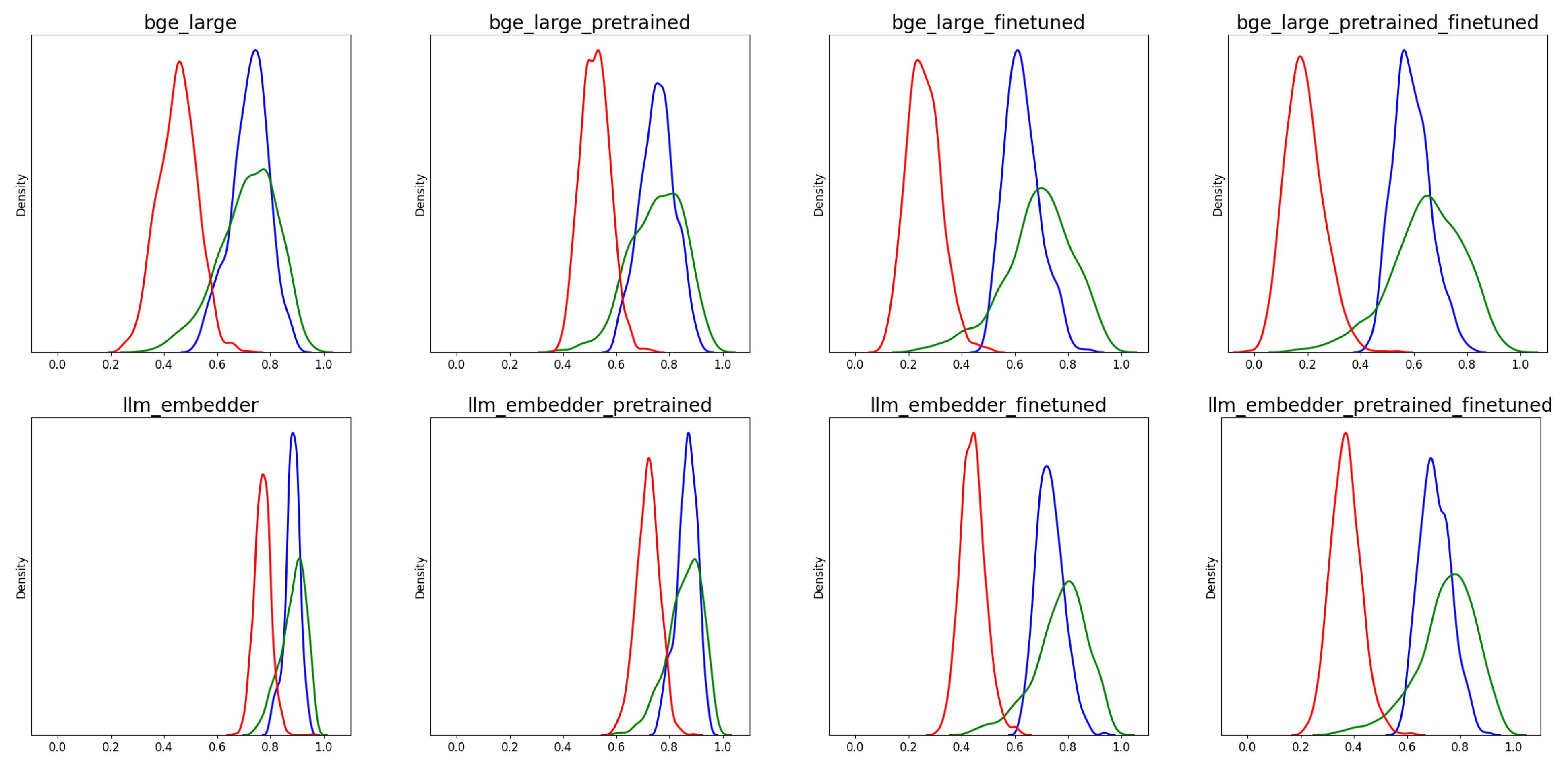
Figure 1: Density plots for telecom dataset $\mathcal{D}$. Red, green and blue indicate distribution of $S_{rand}$, $S_{corr}$ and $S_{topK}$ respectively

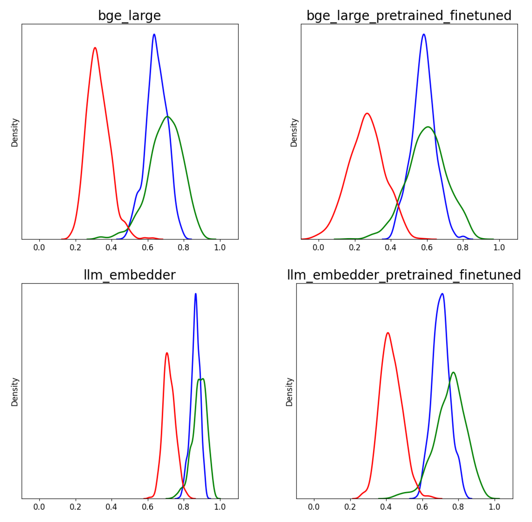
Figure 2: Density plots for SQuAD dataset $\mathcal{D^{\prime}}$. Red, green and blue indicate distribution of $S_{rand}$, $S_{corr}$ and $S_{topK}$ respectively

We report COE (as defined in Section 2.2) for the various models on $\mathcal{D}$ in column 3 of Table 2. The correlation between COE with the top-$K$ accuracy is found to be 0.9. This indicates that the accuracy is related to the overlap between the distributions of the top-$K$ cosine similarities and the distributions of the correct cosine similarities.

The column $\tau({\psi})$ indicates the thresholds which have resulted in the best possible accuracies (as reported in column 6 of Table 2). We observe that the accuracies have slightly reduced on introduction of thresholds. However, this can be interpret as the accuracy obtained with (100-$\psi$) percentage of top-$K$ retrieved results, implying more relevant outcomes for end-users/downstream task.

While it is expected that the correlation between ROE (refer Section 2.2) and top-$K$ accuracy is low, it is of interest to analyse the correlation of ROE with the similarity threshold ($\tau(\psi)$); this is found to be -0.5 and indicating that an higher overlap of top-$K$ with the random is associated with a lower $\tau(\psi)$. These correlations are not obvious - this indicates that for a model to perform well, questions must be well interspersed with answers. This is also reflected in the distribution of embeddings as shown in Figure 1.

On further analysing Figure 1, we notice that the llm_embedder model has a very peaky distribution of cosine similarities (even for $S_{rand})$ similarities. This is indicative of a model with low isotropy. However, despite being less isotropic, the retrieval accuracies of the model is similar to the bge_large model which is more isotropic. The fine tuning of llm_embedder model creates a wider distribution of the cosine similarities indicating better isotropy. Similar patterns are observed for distributions obtained from SQuAD dataset, $\mathcal{D}^{\prime}$ as can be observed from Figure 2.

Embedding Model	Bootstrapped Acc	$I_{A}$, $I_{B}$
gte	83.34 (78.48, 90.0)	27.44, 74.18
bge_large	87.66 (81.0, 94.0)	13.34, 45.72
bge_large_pretrained_finetuned	74.23 (66.0, 83.05)	27.44, 74.18
llm_embedder	86.28 (80.0, 93.52)	13.34, 45.72
llm_embedder_pretrained_finetuned	87.25 (80.48, 92.0)	13.02, 31.67
mpnet	83.64 (76.0, 89.0)	15.33, 77.72
minilm	85.32 (78.0, 91.0)	28.8, 64.38

Table 3: Accuracies and isotropy scores for SQuAD dataset ($\mathcal{D^{\prime}}$), k=5

Retrieval accuracies for SQuAD dataset, $\mathcal{D}^{\prime}$ are reported in Table 3. We observe that the scores for the publicly available models for bge_large and llm_embedder are higher than those for $\mathcal{D}$. This is expected given the QA are not domain specific. We observe that the performance for bge_large reduces significantly using the pre-trained followed by fine-tuned models but improves by a small amount when the same adaptation is considering using llm_embedder. This is perhaps indicative of the difference in the domain specific data included in the original training of the publicly available models but is hard to quantify.

4.2 Isotropy Score Analysis

Table 4 lists the retrieval accuracies for the telecom dataset $\mathcal{D}$, isotropic measures $I_{A}$ and $I_{B}$ of base and adapted models for various transformations (intended to increase isotropy scores and described in Section 2.5).

Looking more carefully at the isotropy scores, the correlation of $I_{A}$ with top-$K$ accuracy is 0.23 whereas with $I_{B}$ is 0.34 for the untransformed embeddings. This indicates there is little correlation of isotropy scores with accuracy. We note that fine-tuning of either the base model or the pre-trained model improves the isotropy score from the publicly available models (refer rows corresponding to bge_large_finetuned, bge_large_pretrained_finetuned, llm_embedder_finetuned, llm_embedder_pretrained_finetuned). However, we can only interpret this as fine-tuning improves isotropy of embeddings but isotropy does not lead to better retrieval performance.

On observing the isotropy scores with and without transformation, we notice that isotropy scores does show an improvement post transformation. The improvement in isotropic metrics is more steep with whitened transformation for both $I_{A}$ and $I_{B}$ than that of the other two. However, we notice that increase in isotropy does not necessarily improve the retrieval accuracies always across models or across isotropy metrics. This is corroborated with the correlation scores reported in the last row of Table 4. This implies, isotropy improvement using transformations alone may not suffice.

Embedding Model	TelecomQuad (Baseline)		TelecomQuad (Standardized)		TelecomQuad (Whitened)		TelecomQuad (PCA)
	Accuracy	$I_{A}$, $I_{B}$	Accuracy	$I_{A}$, $I_{B}$	Accuracy	$I_{A}$, $I_{B}$	Accuracy	$I_{A}$, $I_{B}$
gte	72.55	11.33, 42.4	72.22	11.64, 96.75	69.53	97.59, 99.34	70.85	21.34, 97.49
bge_large	66.87	9.24, 27.81	66.63	9.71, 97.23	70.3	94.65, 99.55	68.43	16.91, 95
bge_large_pretrained	62.64	6.34, 23.77	59.24	6.82, 96.26	63.15	96.25, 99.55	57.02	12.36, 92.75
bge_large_finetuned	81.61	11.45, 40.58	82.66	11.89, 97.54	76.62	98.16, 99.55	78.76	18.09, 97.99
bge_large_pretrained_finetuned	81.67	10.34, 45.27	80.48	10.78, 97.26	76.97	99.19, 99.43	77.46	15.54, 98.35
llm_embedder	70.06	10.83, 14.54	68.26	11.59, 96.83	71.03	88.08, 99.62	68.58	20.5, 96.71
llm_embedder_pretrained	57.12	5.42, 15.4	53.09	5.94, 95.77	63.92	88.77, 99.62	56.55	11.31, 95.77
llm_embedder_finetuned	81.58	13.94, 22.1	82.28	14.66, 97.34	76.57	96.66, 99.61	79.14	20.73, 97.78
llm_embedder_pre-trained_finetuned	80.37	10.74, 25.01	81.2	11.25, 97.32	77.91	97.09, 99.62	79.44	15.82, 98.11
ada_002	75.48	6.64, 25.52	68.83	7.08, 97.09	68.94	88.33, 99.35	69.31	15.67, 93.8
text-embedding-3-small	69.91	6.33, 45.86	67.18	6.79, 93.14	67.86	98.13, 94.96	66.26	14.46, 89.17
text-embedding-3-large	75.96	3.64, 63.78	71.47	4.11, 94.38	70.58	86.87, 96.41	70.94	11.83, 89.12
mpnet	61.49	9.51, 36.41	57.62	10.25, 96.66	57.64	98.89, 97.76	56.39	16.35, 93.72
minilm	67.26	19.43, 26.59	63.99	20.54, 95.56	63.32	98.45, 90.06	62.22	25.67, 95.32
Correlation With Accuracy	(0.23,0.34)		(0.29,0.39)		(0.06, 0.39)		(0.23, 0.47)

Table 4: Accuracy, $I_{A}$ and $I_{B}$ for embeddings under different transformations. The last row shows the correlation of ($I_{A}$,$I_{B}$) with accuracy

Combining these observations, we conclude that fine tuning improves the isotropy but isotropy cannot be attributed to retrieval accuracies. Our studies indicate that this may be the right resolution between the contradictions among studies by [11] and [12] which we have discussed in Section 1.

4.3 Embedding Analysis post Domain Adaptation

As described in Section 2.6, Figures 3(a) and 3(b) shows the distribution of distances $\Delta_{\mathcal{M}}$ and $\Delta_{\mathcal{M^{\prime}}}$ for both bge_large and llm_embedder, respectively. The plots show that post domain-adaptation, the domain adapted embeddings move away from the general domain embeddings. The farthest points between $\mathcal{D}$ and $\mathcal{D^{\prime}}$ on public models is closer than the closest ones post domain adaptation. This is one of the effects of domain adaption and needs further study.

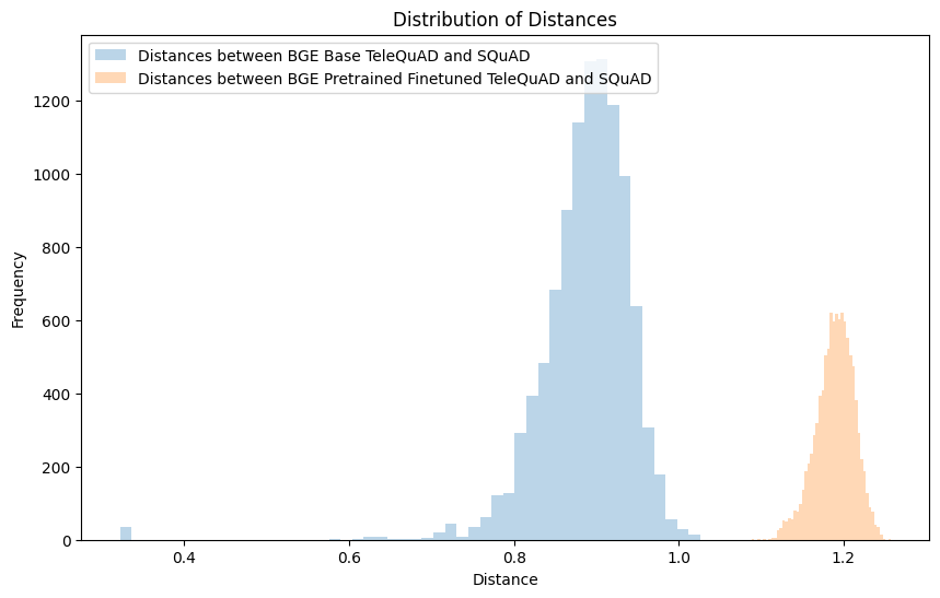
(a) bge-large-en

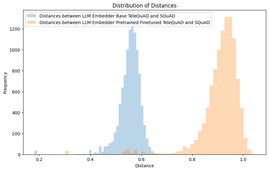
(b) llm-embedder

Figure 3: Distribution of distances for embedding models. Blue histogram represents $\Delta_{\mathcal{M}}$ and orange represents $\Delta_{\mathcal{M}^{\prime}}$ using bge_large (a) and llm_embedder (b) models as $\mathcal{M}$.

5 Conclusions & Future Work

We have reported mean bootstrapped retrieval accuracies along with confidence intervals for various SOTA embedding models. We observe that fine-tuning (with or without pre-training) improves both mean and CI of retrieval accuracies. However, pre-training followed by fine-tuning improves CI further. Choosing thresholds on similarity scores to identify relevant sentences is challenging because of the variation of similarity scores across models. We propose a bootstrapped approach for choosing thresholds and observe that we can significantly reduce the number of retrieved sentences with minimal reduction in retrieval performance. Our proposed cumulative distribution metrics, COE and ROE, to measure overlap between distributions of cosine similarities show strong correlations with retrieval performance and similarity thresholds respectively. We measure isotropy of embeddings using two independent SOTA isotropy metrics. We perform extensive evaluations on embeddings with and without isotropic transformations. We conclude that isotropy can be considered to be neither necessary nor sufficient from a retrieval accuracy perspective. Finally, we observe that with domain adaption, domain specific embedding show improved isotropy scores and move away from general domain embeddings. Our study establishes systematic methods of analysing embeddings in specialised domains. Although we have reported results on telecom domain only, we believe that our approach is generic and can be replicated across other domains too.

Limitations in this study include, extending this work for other domains and other models (such as domain adapt for GPT embeddings). The effect of domain adaptations on embeddings need further study. These can be considered in future work by us and the community.

References

- [1] Nils Reimers and Iryna Gurevych. Sentence-bert: Sentence embeddings using siamese bert-networks. In Proceedings of the 2019 Conference on Empirical Methods in Natural Language Processing and the 9th International Joint Conference on Natural Language Processing (EMNLP-IJCNLP), pages 3982–3992, 2019.
- [2] Jianlv Chen, Shitao Xiao, Peitian Zhang, Kun Luo, Defu Lian, and Zheng Liu. Bge m3-embedding: Multi-lingual, multi-functionality, multi-granularity text embeddings through self-knowledge distillation. arXiv preprint arXiv:2402.03216, 2024.
- [3] Peitian Zhang, Shitao Xiao, Zheng Liu, Zhicheng Dou, and Jian-Yun Nie. Retrieve anything to augment large language models, 2023.
- [4] Shitao Xiao, Zheng Liu, Peitian Zhang, and Niklas Muennighoff. C-pack: Packaged resources to advance general chinese embedding, 2023.
- [5] Bohan Li, Hao Zhou, Junxian He, Mingxuan Wang, Yiming Yang, and Lei Li. On the sentence embeddings from pre-trained language models. In Proceedings of the 2020 Conference on Empirical Methods in Natural Language Processing (EMNLP), pages 9119–9130, 2020.
- [6] Kaitlyn Zhou, Kawin Ethayarajh, Dallas Card, and Dan Jurafsky. Problems with cosine as a measure of embedding similarity for high frequency words. arXiv preprint arXiv:2205.05092, 2022.
- [7] Harald Steck, Chaitanya Ekanadham, and Nathan Kallus. Is cosine-similarity of embeddings really about similarity? In Companion Proceedings of the ACM on Web Conference 2024, pages 887–890, 2024.
- [8] Deven M Mistry and Ali A Minai. A comparative study of sentence embedding models for assessing semantic variation. In International Conference on Artificial Neural Networks, pages 1–12. Springer, 2023.
- [9] Daniel Biś, Maksim Podkorytov, and Xiuwen Liu. Too much in common: Shifting of embeddings in transformer language models and its implications. In Proceedings of the 2021 conference of the North American chapter of the Association for Computational Linguistics: Human Language Technologies, pages 5117–5130, 2021.
- [10] William Timkey and Marten Van Schijndel. All bark and no bite: Rogue dimensions in transformer language models obscure representational quality. arXiv preprint arXiv:2109.04404, 2021.
- [11] Euna Jung, Jungwon Park, Jaekeol Choi, Sungyoon Kim, and Wonjong Rhee. Isotropic representation can improve dense retrieval. In Pacific-Asia Conference on Knowledge Discovery and Data Mining, pages 125–137. Springer, 2023.
- [12] William Rudman and Carsten Eickhoff. Stable anisotropic regularization. arXiv preprint arXiv:2305.19358, 2023.
- [13] William Rudman, Nate Gillman, Taylor Rayne, and Carsten Eickhoff. Isoscore: Measuring the uniformity of embedding space utilization. arXiv preprint arXiv:2108.07344, 2021.
- [14] Feng Hou, Ruili Wang, See-Kiong Ng, Fangyi Zhu, Michael Witbrock, Steven F Cahan, Lily Chen, and Xiaoyun Jia. Anisotropic span embeddings and the negative impact of higher-order inference for coreference resolution: An empirical analysis. Natural Language Engineering, pages 1–22, 2024.
- [15] Mira Ait-Saada and Mohamed Nadif. Is anisotropy truly harmful? a case study on text clustering. In Proceedings of the 61st Annual Meeting of the Association for Computational Linguistics (Volume 2: Short Papers), pages 1194–1203, 2023.
- [16] Nathan Godey, Éric de la Clergerie, and Benoît Sagot. Is anisotropy inherent to transformers? arXiv preprint arXiv:2306.07656, 2023.
- [17] Anton Razzhigaev, Matvey Mikhalchuk, Elizaveta Goncharova, Ivan Oseledets, Denis Dimitrov, and Andrey Kuznetsov. The shape of learning: Anisotropy and intrinsic dimensions in transformer-based models. arXiv preprint arXiv:2311.05928, 2023.
- [18] Sara Rajaee and Mohammad Taher Pilehvar. How does fine-tuning affect the geometry of embedding space: A case study on isotropy. In Findings of the Association for Computational Linguistics: EMNLP 2021, pages 3042–3049, 2021.
- [19] Yunfan Gao, Yun Xiong, Xinyu Gao, Kangxiang Jia, Jinliu Pan, Yuxi Bi, Yi Dai, Jiawei Sun, and Haofen Wang. Retrieval-augmented generation for large language models: A survey. arXiv preprint arXiv:2312.10997, 2023.
- [20] Marius Mosbach, Anna Khokhlova, Michael A Hedderich, and Dietrich Klakow. On the interplay between fine-tuning and sentence-level probing for linguistic knowledge in pre-trained transformers. In Findings of the Association for Computational Linguistics: EMNLP 2020, pages 2502–2516, 2020.
- [21] Sanjeev Arora, Yuanzhi Li, Yingyu Liang, Tengyu Ma, and Andrej Risteski. A latent variable model approach to pmi-based word embeddings. Transactions of the Association for Computational Linguistics, 4:385–399, 2016.
- [22] Jiaqi Mu, Suma Bhat, and Pramod Viswanath. All-but-the-top: Simple and effective postprocessing for word representations. arXiv preprint arXiv:1702.01417, 2017.
- [23] William Rudman, Nate Gillman, Taylor Rayne, and Carsten Eickhoff. Isoscore: Measuring the uniformity of embedding space utilization. In Findings of the Association for Computational Linguistics: ACL 2022, pages 3325–3339, 2022.
- [24] 3GPP release 17. https://www.3gpp.org/specifications-technologies/releases/release-17, 2022. Accessed: 2024-05-19.
- [25] Edward Loper and Steven Bird. Nltk: The natural language toolkit. arXiv preprint cs/0205028, 2002.
- [26] Pranav Rajpurkar, Jian Zhang, Konstantin Lopyrev, and Percy Liang. Squad: 100,000+ questions for machine comprehension of text. arXiv preprint arXiv:1606.05250, 2016.
- [27] Kaitao Song, Xu Tan, Tao Qin, Jianfeng Lu, and Tie-Yan Liu. Mpnet: Masked and permuted pre-training for language understanding. Advances in neural information processing systems, 33:16857–16867, 2020.