Dynamics of the conserved net-baryon density near QCD critical point within QGP profile
Abstract
This paper investigates the dynamics of the net-baryon multiplicity fluctuations near the QCD critical point, within the inhomogeneous temperature and baryon chemical potential profile of quark-gluon plasma from the hydrodynamics. We numerically solve the Langevin dynamics of conserved net-baryon density and borrow the temperature and chemical potential profile from hydrodynamic simulation. It is found that the local systems at different rapidities reach the critical point at different proper times, owing to the inhomogeneous temperature and chemical potential. As a result, we find the pronounced enhancement of the magnitude for the net-baryon multiplicity fluctuations with large rapidity acceptance at the freeze-out surface, which is the consequence of the combined effect of critical slowing down and inhomogeneous profile.
I Introduction
Searching the Quantum Chromodynamics (QCD) critical point is one of the most important goals of the relativistic heavy-ion collisions. The transition from the quark-gluon plasma (QGP) phase to the hadron phase is revealed as a crossover at the vanishing baryon chemical potential () by lattice QCD [1, 2, 3, 4]. While the first-order phase transition together with the critical point is predicted by the effective theories of QCD at finite chemical potential [5, 6, 7, 8]. The most important property of the critical point is the long-range correlation and large fluctuations. As a consequence, the non-monotonic behavior is conjectured as the characteristic signature of the QCD phase transition [9, 10].
The Beam Energy Scan program at RHIC has been dedicated to exploring the QCD phase structure. The preliminary non-monotonic behavior of net-proton multiplicity fluctuations as a function of colliding energy has been observed [11, 12]. However, the statistics of the measurement are insufficient to conclude the observation of this non-monotonicity so far, which is looking forward to the higher statistics in the coming Bean Energy Scan phase two program.
On the other hand, the final confirmation of the existence of the QCD critical point requires the comparison between the experimental measurement and theoretical prediction. After decades of efforts, remarkable progress has been made in the theoretical modeling of the dynamics near the QCD critical point within the complex evolution of the relativistic heavy-ion collisions. Please see e.g., Refs.[13, 14, 15, 16, 17, 18] for recent review. Due to the fast-expanding QGP fireball, the non-equilibrium critical fluctuations become non-trivial compared with the equilibrium ones. For example, the magnitude of the fluctuations is suppressed [19, 20], the sign could be reversed [21], and the largest fluctuations not necessarily correspond to the trajectory closest to the critical point [22]. Subsequently, several models have been developed to incorporate the dynamics of the critical effects. For instance, the dynamics of conserved charge were constructed [23, 24, 25, 26]and non-monotonic behavior of multiplicity fluctuations with respect to acceptance was predicted [25, 26]. To investigate the dynamics of the QGP fireball near the QCD critical point, the dynamics of the critical fluctuations were also coupled to the dynamics of the fireball as an additional degree of freedom, such as the stochastic dynamics of order parameter field in non-equilibrium chiral hydrodynamics [27, 28, 29], the stochastic noise terms in the fluctuating hydrodynamics [30, 31, 32, 17] and the slow mode in the hydro+ [33].
The dynamics of the conserved quantity are of particular interest because the corresponding diffusion process requires time. The correlation between particles far away from each other preserves the early evolution of diffusion [25], and the non-monotonic behavior with respect to acceptance could be regarded as the imprint of the evolving trajectory passing through the critical region. In addition, multi-particle correlation becomes indispensable as the system is extremely close to the critical point. Thus, the dynamics of conserved net-baryon density with higher-order correlation was constructed in the longitudinal Bjorken expansion system with uniform temperature and chemical potential profile [26]. It was found that the pronounced minimum of kurtosis presents at the intermediate rapidity due to the existence of the critical point.
In the realistic context, the temperature and chemical point are not uniform across the QGP profile because of the baryon stopping effects [34, 35]. As a result, different regions of the QGP profile experience distinct trajectories across the critical region [36], and the rapidity dependence is expected to deform non-trivially [37]. In the dynamics of conserved variables, the realistic QGP profile is particularly important because its rapidity dependence on correlation preserves the history along the evolving trajectory. Therefore, it is essential to investigate the rapidity dependence of the multiplicity fluctuations within the more realistic QGP profile. This work studies the dynamics of the conserved net-baryon density near the critical point within the inhomogeneous temperature and chemical potential QGP profile. With the profile obtained from the hydrodynamic simulation, we can study the multiplicity fluctuations at freeze-out hypersurface. It is found that the magnitude of the second-order cumulants and kurtosis enhance significantly at large rapidity, which is the consequence of combined effects of critical slowing down and inhomogeneous QGP profile.
II Model and Setups
To study the dynamics of QCD phase transition, one of the natural and simple dynamical models is just focusing on the dynamics of the order parameter field. However, it was pointed out that the dynamics of conserved baryon density is the slowest mode of the system near the critical point when considering the coupling between baryon density and order parameter field [38]. Therefore, the simplest description of the dynamics near the QCD critical point is only considering the dynamics of conserved baryon density and treating the dynamics of other degrees of freedom as the heat bath.
This study focuses on the -dimensional conserved dynamics of net-baryon density near the QCD critical point along the longitudinal direction in Milne frame, i.e. the proper-time and space-time rapidity :
| (1) |
with the white noise has only one non-zero correlation:
| (2) |
Here, is the diffusion coefficient, is the temperature, and the transverse area is set as following Ref. [24]. The equation of can be derived from the conservation of net-baryon number within the Bjorken flow . Please see Refs. [26, 39] for detail and e.g., Refs. [40, 41, 42] for the further extension.
The effective potential near the critical point can be parameterized as [26]:
| (3) |
where represents the surface tension coefficient and is treated as a constant in this study. The second-order baryon susceptibility , third- and fourth-order coupling coefficients contain two parts: regular part estimated from lattice QCD simulation and singular part () mapped from three-dimensional Ising model () (here are Ising variables). A complete description of the parameterization of the coefficients can be found in Appendix A.
The parametrization of the baryon susceptibility and coupling coefficients on the QCD phase diagram requires the time evolution profiles for the QGP fireball: temperature and chemical potential . The time evolution of the QGP profiles is obtained from the 3+1-d hydrodynamic MUSIC simulation [43], as in Ref.[22]. The initial profiles constructed from the transport model AMPT [44] and the Equation of State are input with the lattice simulation results, incorporating with a critical point [45]. To roughly fit the experimental measurement of Au+Au collisions at 19.6GeV, such as the multiplicity, spectra, and flow, the parameters for the hydrodynamic model are set as [22]: the starting proper time for the AMPT initial condition fm, the starting time for the hydrodynamic evolution fm, the specific shear and bulk viscosity , and the switching energy density from QGP to hadronic phase . We fix the position of the critical point as . To illustrate the effects of the realistic QGP profile, we perform the simulation with two scenarios:
-
1.
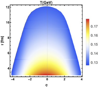
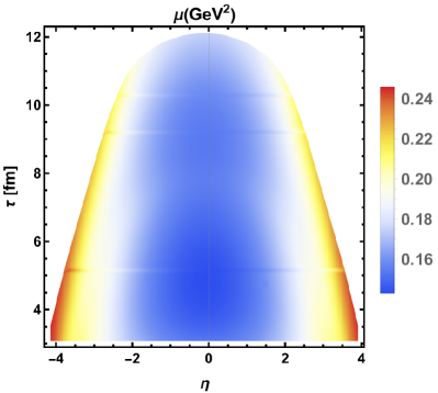
Scenario I: We extract the temperature and chemical potential along the longitudinal direction by averaging the temperature and chemical potential profiles over the whole QGP fireball with the energy density as the weight: and . and profile from hydrodynamic simulation at 19.6GeV with centrality is presented in Figs. 1
-
2.
Scenario II: For comparison, we also study the net-baryon density dynamics within the uniformed background of temperature and chemical potential along the longitudinal direction. The temperature and chemical potential along the longitudinal direction are fixed the ones at : and .
As depicted in the upper panel of Figs. 1, the temperature is highest at the center of the fireball and decreases with increasing rapidity , and this behavior becomes smoother as a function of proper time . Conversely, the chemical potential reaches its minimum at the fireball’s center and exhibits a larger value for higher rapidity. This behavior illustrates the baryon-stopping effects along the longitudinal direction. This study only focuses on the dynamics with the QGP fireball, there is no value outside the fireball as the system has freeze-out and turned into the hadronic phase.
It requires the solution of the Eq.(1) to obtain the time evolution of the net-baryon density along the longitudinal axis. In the case of the linear stochastic diffusion equation, without cubic and quartic terms of Eq.(1), the dynamics of net-baryon density can be solved analytically. However, it requires numerical simulation of the non-linear equation Eq.(1) when considering cubic and quartic terms. One of the most popular algorithms for this diffusive stochastic equation is the explicit Forward or Backward Euler Method. However, the Euler Method is conditional stable and the numerical simulation is extremely inefficient near the critical point. In this work, we perform, the numerical simulation of Eq.(1) with the Saul’yev scheme, which is an explicit unconditional stable scheme. In 1957, V.K.Saul’yev proposed the so-called asymmetric methods in the simulation of diffusion equation [46, 47] and has been successfully implemented in the study of Cahn-Hilliard equation [48]. For the detailed numerical implementation of Eq.(1), please see Appendix.B.
With the configuration of the net-baryon density after solving Eq.(1), we are able to study the dynamics of the multiplicity fluctuations, which can be calculated as follows:
| (4) |
and . Here denotes the multiplicity of net-baryon, represents averaging over the events and the multiplicity event-by-event fluctuations are defined as .
After the evolution of the net-baryon density with the QGP profile, systems freeze out and turn into the hadronic phase when the energy density is below the switching energy density . The freeze-out hyper-surface from the hydrodynamic simulation is employed and shown as the edge of the QGP profile in Figs.1. To calculate the multiplicity fluctuations after freeze-out, we employ the Cooper-Frye formula [49]:
| (5) |
where is the spin degeneracy and we take the Boltzmann approximation:
| (6) |
Following Refs. [30, 39, 50], we employ the Bjorken limit: and , with and is transverse momentum. Therefore, the expression of reads:
| (7) |
where is the irregular modified Bessel function of order-. The integral over the transverse space is represented by [24]. As there is only one fluctuating variable in this framework, following Ref.[39], the multiplicity fluctuations is obtained as
| (8) |
by considering the definition of the susceptibility in Milne frame. Here, the integration over is performed at the edge of the hydrodynamic profile, the freeze-out surface. The fluctuations of the net-baryon density , as well as the temperature , chemical potential and susceptibility are also extracted from the hypersurface. Various orders of the cumulants of the multiplicity fluctuations are calculated as Eq.(II) accordingly.
III RESULT AND DISCUSSION
This work focuses on the inhomogeneous QGP background effects on the dynamics of the conserved net-baryon fluctuations near the QCD critical point. The inhomogeneous temperature and chemical potential profile are extracted from the hydrodynamic simulation. This section will show the net-baryon susceptibility and coupling constants within the inhomogeneous profile, as well as its impact on the dynamics of the net-baryon density near the QCD critical point.
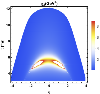
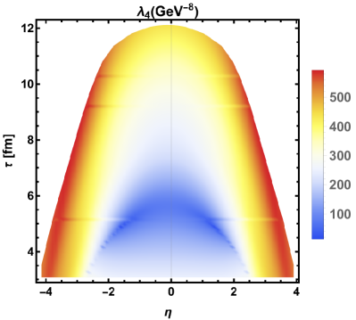
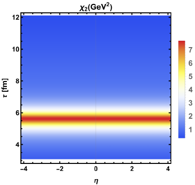
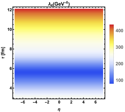
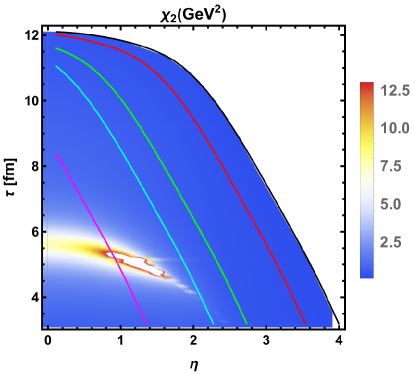
Figs.2 plot the time evolution of second-order net-baryon susceptibility and fourth-order coupling coefficient across the QGP profile. Due to the inhomogeneous temperature and chemical potential across rapidity space 1, the local regions at different rapidities reach the critical point at varying times. Consequently, the strength of critical effects varies along the rapidity axis for a given proper time. As shown in Fig.2, the local regions at finite rapidities (around ) are the points closest to the QCD critical point, owing to the combined influence of the inhomogeneous and . Therefore, it is natural to expect that multiplicity fluctuations would exhibit nontrivial behavior in response. For the comparison, Scenario II, the time evolution of the coefficients for the uniform temperature and chemical potential has also been shown in Fig.3, where the proper time evolution of and are uniform across the space.
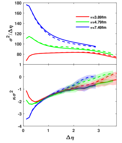
With the temperature and chemical potential profile obtained from hydrodynamic simulation, it is possible to study the net-baryon number fluctuations during the QGP evolution. Let’s start with the rapidity dependence of the net-baryon number fluctuations. Figs.4 show the rapidity dependence of the net-baryon number fluctuations with fixed proper time and fm, respectively. The second order net-baryon number cumulant (kurtosis ) shows non-monotonic behavior with increasing rapidity and reaches a maximum (minimum) at small , which agrees with previous studies [25, 26]. One of the most important properties of the dynamics for the conserved variable is that the diffusion process consumes time (Please see Ref. [25] for detail). As a result, the correlation between particles with small encodes the late-stage dynamics of diffusion, while the one with large preserves the early evolution of diffusion. As the system scans the critical regime, the susceptibility exhibits a peak with increasing proper time . Therefore, the correlation behaves non-monotonically with increasing rapidity interval , which can be regarded as the imprints from the critical fluctuations. We also compare the and in uniform (Scenario II, solid curves) with inhomogeneous (Scenario I, dashed curves) profile. In the case of second-order cumulant , the difference between Scenario II and I is negligible. For kurtosis, the discrepancy is also small at small rapidity but becomes significant for large rapidity. This can be understood that the difference of the transport coefficients ( and ) in Eq.(1) between Scenario I and II becomes pronounced at large , by comparing Figs.2 and 3.
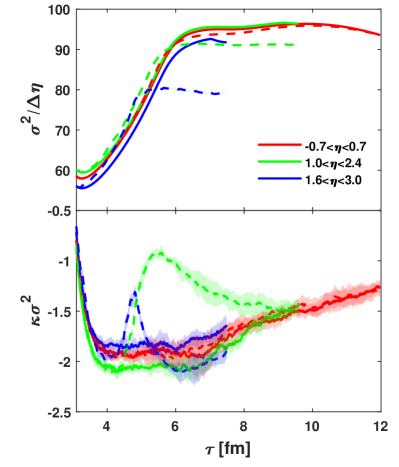
Since the realistic inhomogeneous QGP profile has an impact on the number fluctuations at large rapidity, let’s focus on the time evolution of the system fluctuations at different . With the number fluctuations obtained from Eq.(II), Figs.5 present the time evolution of and with different intervals both for uniform (Scenario II) and inhomogeneous (Scenario I) profile. In these figures, solid curves represent the time evolution of the fluctuations with realistic inhomogeneous QGP profile (Scenario I), while the dashed curves correspond to the uniform profile case (Scenario II). As shown in Figs.5, the discrepancy between these two cases is negligible for midrapidity interval (), while becomes significant at large rapidity intervals ( and ) 111Noted that the integral interval of in Figs.4 is from to . The difference between Scenario I and II is small when the integration is also performed from to for the time evolution of in Figs.5. This is consistent with Figs.4 and the difference between Scenario I and II in different rapidity is smeared out from to . .
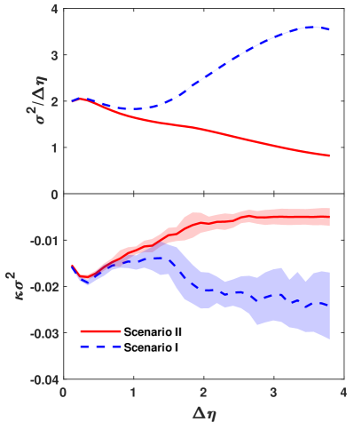
The hydrodynamic simulation provides us with the temperature and chemical potential profile. After the energy density drops and below the switching energy density , QGP evolution terminates and freezes out into the hadronic phase. This procedure defines the freeze-out hypersurface, shown as the edge of the QGP fireball of the () plane in Figs.1, and enables us to study the multiplicity fluctuations at the freeze-out hyper-surface. Following Eq.(8), net-baryon multiplicity fluctuations at the freeze-out surface are calculated and shown in Figs.6. For illustrative purposes, we present the multiplicity fluctuations obtained with the uniform and profile (Scenario II) but still at the edge of the profile 1. Note that the freeze-out surface for Scenario II is not the edge of the profile 1, and the solid curves are presented for comparison. In the scenario of a uniform temperature and chemical potential profile, second order fluctuations (kurtosis ) display an increase (decrease) first followed by a rapid decline (increase) with increasing rapidity interval , exhibiting a maximum (minimum) at small values of rapidity interval . This behavior is consistent with studies on diffusive dynamics near the critical point [25, 26], suggesting that the correlation with large preserves the early dynamics of diffusion. On the contrary, and in the case of the realistic QGP profile deviate significantly with uniform temperature and chemical potential case at large rapidity interval . As shown in Figs.1, the fluctuations with different rapidity at the freeze-out surface are determined by the dynamics with different time . The significant enhancement (decrease) of and is a result of the dynamics occurring at small .
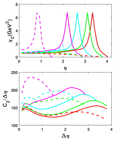
To see this, it is instructive to study the rapidity dependence of the multiplicity fluctuations before freeze-out. This can be achieved by moving the freeze surface backward to the smaller region. In Fig.7, the curves in QGP fireball are depicted, along which the variables at smaller region are extracted. Figs.8 show the susceptibility and along the curves in Fig.7. Here , where the integral is performed along the curves in Fig.7. With increasing in Scenario I, one could see the peak of susceptibility only exhibits along the curves with small and , and been significantly suppressed near the freeze-out surface. This is the impact of the inhomogeneous QGP profile, in which the system passes through the critical regime and a pulse of the susceptibility appears and vanishes rapidly. On the other hand, during the process of diffusion, the pulse of the susceptibility near the QCD critical point results in the large fluctuations at small , as shown in the dashed-magenta curve in the lower panel of Figs.8. The large fluctuations smears and diffuses with increasing proper time and rapidity, but can not catches up with the rapid decreasing , which is known as the critical slowing down effects. In short, the evolution of the and profiles drives the susceptibility passing through the critical point, while the critical slowing down effects preserve the memory of the large net-baryon density fluctuations at the critical point. Consequently, the fluctuations in Eq.(8) behave with pronounced enhancement at large rapidity intervals. On the contrary, one could see the susceptibility always has a peak and moves to larger in Scenario II, which is expected in Fig.3. Therefore, the fluctuations at Eq.(8) drop down rapidly with increasing even with the diffusion of net-baryon density (lower panel of Figs.8).
IV Conclusion and Outlook
This work studies the conserved dynamics of the net-baryon multiplicity fluctuations near the QCD critical point with the inhomogeneous temperature and chemical potential profile. The dynamics of conserved net-baryon density are based on the numerical simulation of the 1+1-dimensional stochastic diffusion equation. The realistic QGP profile is obtained by the hydrodynamic simulation and the susceptibilities in the diffusion equation are constructed based on the temperature and chemical potential profile. In this context, the QGP profile is inhomogeneous and the susceptibilities are non-trivial across the proper time and rapidity plane. As discovered by the early studies, the fluctuations of the conserved net-baryon density behave non-monotonically with the increasing rapidity interval, owing to the fact that the correlation function in the diffusion process preserves the evolution history at large rapidity interval. It is found that the influence of the inhomogeneous profile is negligible at small rapidity but relatively pronounced at large rapidity, as the susceptibility in the realistic case deviates from the case of the uniform profile at large rapidity. Furthermore, the fluctuations on the freeze-out hypersurface have also been investigated. Comparing the case with a uniform QGP profile, the magnitudes of second-order cumulants as well as kurtosis in inhomogeneous profile present significant enhancement at large rapidity. This is the result of the combined effect of critical slowing down and inhomogeneous profile.
Finally, it deserves to be pointed out that this study of the critical fluctuations is based on a simplified model, where only the 1+1-dimensional conserved net-baryon density is considered. Other degrees of freedom in hydrodynamic evolution have not been considered comprehensively, and are only regarded as the background. As shown in this paper, the dynamical simulation of the relevant quantity with a realistic setup is essential for comparison with experimental measurement. For example, the hydrodynamics coupling with the additional slow modes has been developed [33], and further incorporating the higher order slow modes, their extension at freeze-out surface [52], and corresponding phenomenological study are required for the persuasive prediction.
Acknowledgments
The author would like to thank Shian Tang for his contribution at the beginning of this study and discussion with Huichao Song. This work is supported by the NSFC under grant No. 12305143 and the China Postdoctoral Science Foundation under Grant No. 2023M731467.
Appendix A Parametrization
The coefficients of the Eq.(1) require to be specified for the simulation of net-baryon density near the QCD critical point. According to the universal analysis, one can obtain the diffusion coefficient , second-order baryon susceptibility , and third- and fourth-order coupling coefficients from the mapping three-dimensional Ising model. Following Refs. [25, 26], these coefficients include regular and singular parts:
| (9) |
where the regular coefficients read
With the susceptibility, one has the diffusion coefficient near the critical point. and surface tension coefficient are treated as constants: and .
The regular susceptibilities are obtained by interpolating interpolate between the regular susceptibilities at hadronic phase and QGP phase
where the interpolating function is and the width of the transition region is set as GeV. Following Ref. [39], the second-order susceptibility for hadronic phase and for QGP phase, where we set the low-temperature limit GeV and the high-temperature limit GeV. For the fourth order susceptibility, at hadronic phase and from the lattice simulation [53, 54]. We assume the third-order susceptibility has the relation from Refs. [55, 56]. Finally, we have the regular susceptibilities both for the hadronic and QGP phases:
The critical contributions and are constructed from the cumulants of Ising model
| (10) |
where is mapping constant and chosen as in this work. is the constant for the dimensional consistency and is set as GeV. The dimensionaless coupling constants and have values range (0,8) and (4,20), respectively [57]. and are used in this study. The second-order cumulant of the Ising model reads [20, 25]
| (11) |
where the normalization constants are . On the phase diagram near the critical point, the distance and angle to the critical point are calculated with the equations
| (12) |
The Ising variables () are connected to the temperature and chemical potential of the QCD system by the mapping:
| (13) |
where and are the critical temperature and chemical potential, respectively. and represent the widths of the critical region of the QCD phase diagram, and are the ones in the Ising model. These are non-universal parameters and we use GeV, in this work. The temperature and chemical potential of the QGP profile are borrowed from hydrodynamic simulation, which is addressed in Sec. II
Appendix B Numerical details of Eq.(1)
This appendix presents the details of the numerical simulation of Eq.(1) and its verification by comparison with the analytical calculation in the linear limit of Eq.(1).
One of the most popular algorithms for this diffusive stochastic equation is the explicit Forward or Backward Euler Method. In this numerical algorithm, Eq.(1) can be discretized in an explicit form: , where the next time step only shown in the left-hand side and can be obtained explicitly. However, this scheme is conditionally stable because it is only an approximation to Eq.(1), error will gradually accumulate and eventually lead to instability. The situation is exacerbated as the system approaches the critical point. To attain stable solutions, the temporal step should be significantly smaller than the spatial step, such as for diffusion equation , namely the conditional stable. This makes the numerical simulation extremely inefficient.
This work implements the numerical simulation with Saul’yev scheme [46, 47], where this equation can be discretized as
| (16) |
where and denotes the discretization of the higher order terms . The noise term is discretized into , corresponding to the Gaussian white noise with unit variance. is the net-baryon density at proper time and rapidity . In this simulation, the increment in the proper time is chosen as fm and the spacing of the rapidity is . The grid size of the simulation is with . The initial proper time is fm with the initial condition: .
As shown in Eq.(B), the net-baryon density for the next temporal step at grid site only depends on the ones of time step , expect and at right hand side of Eq.(B). Therefore, can be computed explicitly, with the boundary condition of the cell given, and the simulation starts the cell from the left to the right . On the other hand, the freeze-out hyper-surface of the QGP profile naturally provides the boundary of the simulation. At the edge of this hypersurface, we employ the boundary condition as follows: evolving the net-baryon density with Eq.(B), but replacing the cell outside (e.g.,) with the closest boundary (e.g.,) if the cell fall at the right side of the profile.
To verify the implemented numerical scheme Eq.(B), the dynamics of the net-baryon density without the higher order terms are investigated:
| (17) |
with noise (15). This is the stochastic diffusion equation employed in the previous works [25, 58] and the corresponding analytical solution of second-order baryon multiplicity fluctuations reads
| (18) |
where and is the derivative of over the proper time.
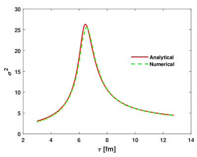
It requires the time evolution of and for the comparison of analytical second order multiplicity Eq. (B) with the numerical results of Eq. (17) with the algorithm Eq.(B). This can be constructed following the method of Eq. (A) in Append A. Here, the time evolution of temperature is not obtained from QGP profile, but we employ the Hubble-like expansion [25, 58], and fixed chemical potential GeV, with GeV and . In this calculation, temperature and chemical potential are constant across the rapidity space. Fig.9 shows the comparison of the time evolution of obtained both from numerical simulation and analytical calculation. The agreement between these two methods verifies the reliability of the Saul’yev scheme in the simulation of Eq. (1).
References
- Aoki et al. [2006] Y. Aoki, G. Endrodi, Z. Fodor, S. D. Katz, and K. K. Szabo, Nature 443, 675 (2006), arXiv:hep-lat/0611014 .
- Ding et al. [2015] H.-T. Ding, F. Karsch, and S. Mukherjee, Int. J. Mod. Phys. E 24, 1530007 (2015), arXiv:1504.05274 [hep-lat] .
- Bazavov et al. [2019] A. Bazavov, F. Karsch, S. Mukherjee, and P. Petreczky (USQCD), Eur. Phys. J. A 55, 194 (2019), arXiv:1904.09951 [hep-lat] .
- Ratti [2018] C. Ratti, Rept. Prog. Phys. 81, 084301 (2018), arXiv:1804.07810 [hep-lat] .
- Fischer [2019] C. S. Fischer, Prog. Part. Nucl. Phys. 105, 1 (2019), arXiv:1810.12938 [hep-ph] .
- Fukushima and Hatsuda [2011] K. Fukushima and T. Hatsuda, Rept. Prog. Phys. 74, 014001 (2011), arXiv:1005.4814 [hep-ph] .
- Fukushima and Sasaki [2013] K. Fukushima and C. Sasaki, Prog. Part. Nucl. Phys. 72, 99 (2013), arXiv:1301.6377 [hep-ph] .
- Fu [2022] W.-j. Fu, Commun. Theor. Phys. 74, 097304 (2022), arXiv:2205.00468 [hep-ph] .
- Stephanov [2011] M. A. Stephanov, Phys. Rev. Lett. 107, 052301 (2011), arXiv:1104.1627 [hep-ph] .
- Athanasiou et al. [2010] C. Athanasiou, K. Rajagopal, and M. Stephanov, Phys. Rev. D 82, 074008 (2010), arXiv:1006.4636 [hep-ph] .
- Adam et al. [2021] J. Adam et al. (STAR), Phys. Rev. Lett. 126, 092301 (2021), arXiv:2001.02852 [nucl-ex] .
- Abdallah et al. [2021] M. Abdallah et al. (STAR), Phys. Rev. C 104, 024902 (2021), arXiv:2101.12413 [nucl-ex] .
- Asakawa and Kitazawa [2016] M. Asakawa and M. Kitazawa, Prog. Part. Nucl. Phys. 90, 299 (2016), arXiv:1512.05038 [nucl-th] .
- Bzdak et al. [2020] A. Bzdak, S. Esumi, V. Koch, J. Liao, M. Stephanov, and N. Xu, Phys. Rept. 853, 1 (2020), arXiv:1906.00936 [nucl-th] .
- Bluhm et al. [2020] M. Bluhm et al., Nucl. Phys. A 1003, 122016 (2020), arXiv:2001.08831 [nucl-th] .
- Wu et al. [2021] S. Wu, C. Shen, and H. Song, Chin. Phys. Lett. 38, 081201 (2021), arXiv:2104.13250 [nucl-th] .
- An et al. [2022] X. An et al., Nucl. Phys. A 1017, 122343 (2022), arXiv:2108.13867 [nucl-th] .
- Du et al. [2024a] L. Du, A. Sorensen, and M. Stephanov (2024) arXiv:2402.10183 [nucl-th] .
- Berdnikov and Rajagopal [2000] B. Berdnikov and K. Rajagopal, Phys. Rev. D 61, 105017 (2000), arXiv:hep-ph/9912274 .
- Nonaka and Asakawa [2005] C. Nonaka and M. Asakawa, Phys. Rev. C 71, 044904 (2005), arXiv:nucl-th/0410078 .
- Mukherjee et al. [2015] S. Mukherjee, R. Venugopalan, and Y. Yin, Phys. Rev. C 92, 034912 (2015), arXiv:1506.00645 [hep-ph] .
- Tang et al. [2023] S. Tang, S. Wu, and H. Song, Phys. Rev. C 108, 034901 (2023), arXiv:2303.15017 [nucl-th] .
- Nahrgang et al. [2019] M. Nahrgang, M. Bluhm, T. Schaefer, and S. A. Bass, Phys. Rev. D 99, 116015 (2019), arXiv:1804.05728 [nucl-th] .
- Nahrgang and Bluhm [2020] M. Nahrgang and M. Bluhm, Phys. Rev. D 102, 094017 (2020), arXiv:2007.10371 [nucl-th] .
- Sakaida et al. [2017] M. Sakaida, M. Asakawa, H. Fujii, and M. Kitazawa, Phys. Rev. C 95, 064905 (2017), arXiv:1703.08008 [nucl-th] .
- Pihan et al. [2023] G. Pihan, M. Bluhm, M. Kitazawa, T. Sami, and M. Nahrgang, Phys. Rev. C 107, 014908 (2023), arXiv:2205.12834 [nucl-th] .
- Nahrgang et al. [2011] M. Nahrgang, S. Leupold, C. Herold, and M. Bleicher, Phys. Rev. C 84, 024912 (2011), arXiv:1105.0622 [nucl-th] .
- Nahrgang et al. [2013] M. Nahrgang, C. Herold, S. Leupold, I. Mishustin, and M. Bleicher, J. Phys. G 40, 055108 (2013), arXiv:1105.1962 [nucl-th] .
- Herold et al. [2014] C. Herold, M. Nahrgang, Y. Yan, and C. Kobdaj, J. Phys. G 41, 115106 (2014), arXiv:1407.8277 [hep-ph] .
- Kapusta et al. [2012] J. I. Kapusta, B. Muller, and M. Stephanov, Phys. Rev. C 85, 054906 (2012), arXiv:1112.6405 [nucl-th] .
- An et al. [2020] X. An, G. Başar, M. Stephanov, and H.-U. Yee, Phys. Rev. C 102, 034901 (2020), arXiv:1912.13456 [hep-th] .
- An et al. [2021] X. An, G. Başar, M. Stephanov, and H.-U. Yee, Phys. Rev. Lett. 127, 072301 (2021), arXiv:2009.10742 [hep-th] .
- Stephanov and Yin [2018] M. Stephanov and Y. Yin, Phys. Rev. D 98, 036006 (2018), arXiv:1712.10305 [nucl-th] .
- Shen and Schenke [2018] C. Shen and B. Schenke, Phys. Rev. C 97, 024907 (2018), arXiv:1710.00881 [nucl-th] .
- Du et al. [2024b] L. Du, H. Gao, S. Jeon, and C. Gale, Phys. Rev. C 109, 014907 (2024b), arXiv:2302.13852 [nucl-th] .
- Du et al. [2021] L. Du, X. An, and U. Heinz, Phys. Rev. C 104, 064904 (2021), arXiv:2107.02302 [hep-ph] .
- Brewer et al. [2018] J. Brewer, S. Mukherjee, K. Rajagopal, and Y. Yin, Phys. Rev. C 98, 061901 (2018), arXiv:1804.10215 [hep-ph] .
- Son and Stephanov [2004] D. T. Son and M. A. Stephanov, Phys. Rev. D 70, 056001 (2004), arXiv:hep-ph/0401052 .
- Ling et al. [2014] B. Ling, T. Springer, and M. Stephanov, Phys. Rev. C 89, 064901 (2014), arXiv:1310.6036 [nucl-th] .
- Chao and Schaefer [2021] J. Chao and T. Schaefer, JHEP 01, 071, arXiv:2008.01269 [hep-th] .
- Chao and Schaefer [2023] J. Chao and T. Schaefer, JHEP 06, 057, arXiv:2302.00720 [hep-ph] .
- Hu [2024] J. Hu, arXiv e-prints , arXiv:2403.15825 (2024), arXiv:2403.15825 [cond-mat.stat-mech] .
- Shen et al. [2016] C. Shen, Z. Qiu, H. Song, J. Bernhard, S. Bass, and U. Heinz, Comput. Phys. Commun. 199, 61 (2016), arXiv:1409.8164 [nucl-th] .
- Lin et al. [2005] Z.-W. Lin, C. M. Ko, B.-A. Li, B. Zhang, and S. Pal, Phys. Rev. C 72, 064901 (2005), arXiv:nucl-th/0411110 .
- Parotto et al. [2020] P. Parotto, M. Bluhm, D. Mroczek, M. Nahrgang, J. Noronha-Hostler, K. Rajagopal, C. Ratti, T. Schäfer, and M. Stephanov, Phys. Rev. C 101, 034901 (2020), arXiv:1805.05249 [hep-ph] .
- Saul’yev [1957] V. K. Saul’yev, Dokl. Akad. Nauk SSSR 115, 1077 (1957).
- Saul’yev [1964] V. K. Saul’yev, Integration of Equations of Parabolic Type by the Method of Nets (Pergamon Press, Oxford, 1964).
- Yang et al. [2022] J. Yang, Y. Li, C. Lee, H. G. Lee, S. Kwak, Y. Hwang, X. Xin, and J. Kim, International Journal of Mechanical Sciences 217, 106985 (2022).
- Cooper and Frye [1974] F. Cooper and G. Frye, Phys. Rev. D 10, 186 (1974).
- Kapusta and Torres-Rincon [2012] J. I. Kapusta and J. M. Torres-Rincon, Phys. Rev. C 86, 054911 (2012), arXiv:1209.0675 [nucl-th] .
- Note [1] Noted that the integral interval of in Figs.4 is from to . The difference between Scenario I and II is small when the integration is also performed from to for the time evolution of in Figs.5. This is consistent with Figs.4 and the difference between Scenario I and II in different rapidity is smeared out from to .
- Pradeep and Stephanov [2023] M. S. Pradeep and M. Stephanov, Phys. Rev. Lett. 130, 162301 (2023), arXiv:2211.09142 [hep-ph] .
- Cheng et al. [2009] M. Cheng et al., Phys. Rev. D 79, 074505 (2009), arXiv:0811.1006 [hep-lat] .
- Bazavov et al. [2017] A. Bazavov et al., Phys. Rev. D 95, 054504 (2017), arXiv:1701.04325 [hep-lat] .
- Motornenko et al. [2020] A. Motornenko, J. Steinheimer, V. Vovchenko, S. Schramm, and H. Stoecker, Phys. Rev. C 101, 034904 (2020), arXiv:1905.00866 [hep-ph] .
- Mukherjee et al. [2017] A. Mukherjee, J. Steinheimer, and S. Schramm, Phys. Rev. C 96, 025205 (2017), arXiv:1611.10144 [nucl-th] .
- Tsypin [1994] M. M. Tsypin, Phys. Rev. Lett. 73, 2015 (1994).
- Wu and Song [2019] S. Wu and H. Song, Chin. Phys. C 43, 084103 (2019), arXiv:1903.06075 [nucl-th] .