Hybrid Beamforming Design for Near-Field ISAC with Modular XL-MIMO

Chunwei Meng, Dingyou Ma, Zhaolin Wang, Yuanwei Liu, Zhiqing Wei, Zhiyong Feng C. Meng, D. Ma, Z. Wei, and Z. Feng are with the Key Laboratory of Universal Wireless Communications, Ministry of Education, Beijing University of Posts and Telecommunications, Beijing 100876, China (e-mail: {mengchunwei, dingyouma, weizhiqing, fengzy}@bupt.edu.cn). Z. Wang and Y. Liu are with the School of Electronic Engineering and Computer Science, Queen Mary University of London, London E1 4NS, U.K. (e-mail: {zhaolin.wang, yuanwei.liu}@qmul.ac.uk).
Abstract

A novel modular extremely large-scale multiple-input-multiple-output (XL-MIMO) integrated sensing and communication (ISAC) framework is proposed in this paper. We consider a downlink ISAC scenario and exploit the modular array architecture to enhance the communication spectral efficiency and sensing resolution while reducing the channel modeling complexity by employing the hybrid spherical and planar wavefront model. Considering the hybrid digital-analog structure inherent to modular arrays, we formulate a joint analog-digital beamforming design problem based on the communication spectral efficiency and sensing signal-to-clutter-plus-noise ratio (SCNR). By exploring the structural similarity of the communication and sensing channels, it is proved that the optimal transmit covariance matrix lies in the subspace spanned by the subarray response vectors, yielding a closed-form solution for the optimal analog beamformer. Consequently, the joint design problem is transformed into a low-dimensional rank-constrained digital beamformer optimization. We first propose a manifold optimization method that directly optimizes the digital beamformer on the rank-constrained Stiefel manifold. Additionally, we develop an semidefinite relaxation (SDR)-based approach that relaxes the rank constraint and employ the randomization technique to obtain a near-optimal solution. Simulation results demonstrate the effectiveness of the proposed modular XL-MIMO ISAC framework and algorithms, also providing valuable insights: i) The widely-spaced modular array achieves higher communication spectral efficiency than the collocated array under the same SCNR threshold; ii) The SDR-based algorithm achieves better performance, while the manifold optimization method offers lower computational complexity; iii) Key system parameters, such as the number of RF chains, subarray scale, non-line-of-sigh paths, and communication-sensing channel correlation, significantly impact the ISAC performance.

Index Terms:
Hybrid beamforming, hybrid spherical and planar wavefront model, integrated snesing and communication, modular extremely large-scale MIMO.

I Introduction

The sixth generation wireless systems (6G) have been envisioned as a vital enabler for numerous emerging applications, such as intelligent manufacturing and smart transportation[1, 2]. The challenging problem is to satisfy the requirements of these applications for high-capacity communications and high-resolution sensing, which motivates the development of integrated sensing and communications (ISAC) technologies. The advant of extremely large-scale multiple-input and multiple-output (XL-MIMO) and the exploration of millimeter wave (mmWave)/sub- terahertz (THz) frequency bands in 6G systems lead to a growing convergence between communication and sensing in terms of channel characteristics and signal processing techniques. This convergence makes it feasible to achieve high-precision sensing and high-speed communication simultaneously using integrated waveforms and hardware platforms, offering several advantages such as reduced hardware costs, improved spectral efficiency, and mutual benefits between sensing and communication functionalities.

However, the large array aperture and high operating frequencies adopted in 6G systems significantly extend the Rayleigh distance, making it more likely for communication users and sensing targets to reside in the near-field region[3]. The near-field effect not only invalidates the traditional far-field assumption-based propagation channel models but also introduces new opportunities and challenges for ISAC techniques. The work in [4] revealed that the near-field effect can potentially enhance both communication and sensing performance. However, [4] also shows that the near-field effect introduces new coupling between the two functionalities, necessitating efficient near-field beamforming designs to strike a performance balance. In [5], the authors proposed a near-field ISAC framework that exploits the additional distance dimension for optimal waveform design, showcasing performance gains over conventional far-field ISAC systems. Building upon this, [6] proposed an efficient iterative near-field beamforming algorithm for multi-target detection, demonstrating significant improvements in localization accuracy compared to traditional far-field techniques. Furthermore, the authors in [7] conducted a comprehensive performance analysis for near-field ISAC systems in both uplink and downlink scenarios, characterizing the achievable performance regions under sensing-centric, communications-centric, and Pareto optimal designs. Despite these advancements, the high model and computational complexity, along with the substantial hardware deployment costs associated with near-field XL-MIMO ISAC systems, pose significant challenges for practical implementation in realistic scenarios[4].

To address these challenges, a novel modular XL-MIMO architecture, also known as widely-spaced multi-subarray (WSMS), has recently emerged as a promising solution[8, 9, 10, 11, 12]. This architecture consists of multiple modular subarrays, each composed of a flexible number of array elements with typical half-wavelength spacing, while the subarrays themselves are separated by relatively large distances[9]. The modular XL-MIMO architecture offers several advantages, such as reduced hardware costs, lower power consumption, and ease of flexible deployment in practical scenarios[12]. Moreover, the enlarged array aperture resulting from the wide spacing between subarrays exhibits a larger near-field region, potentially enhancing the performance of near-field ISAC systems. The studies have demonstrated that modular XL-MIMO, compared to collocated arrays, exhibits a more pronounced near-field effect[9], provides both inter-path and intra-path multiplexing gains to improve spectrum efficiency[8], and better adapts to the spatial non-stationarity of the channel[13]. Furthermore, the pronounced near-field effect of modular XL-MIMO also offers significant advantages for sensing. In [12], the authors investigated the potential of near-field localization with modular XL-MIMO by analyzing the Cramér-Rao Bound (CRB) for angle and range estimation, revealing that the increased array aperture and angular span of the modular array significantly enhance the near-field localization performance compared to traditional collocated arrays.

Despite the benefits of modular XL-MIMO for both near-field communication and sensing, the design and optimization of modular XL-MIMO ISAC systems remain unexplored. One of the major challenges lies in the beamforming design for downlink ISAC scenarios, where the partially-connected hybrid digital and analog architecture imposes an additional block-diagonal constraint on the analog beamformer, leading to an intractable non-convex optimization problem. The authors in [14] proposed a two-stage hybrid beamforming (HBF) method, where the analog stage computes the contribution of each submatrix on the diagonal elements of the analog beamformer to the communication spectral efficiency, and an alternating optimization algorithm is employed to solve the problem. However, this approach is not applicable to ISAC systems, as the coupled performance of communication and sensing makes it complex and impractical to separately quantify the contribution of each diagonal submatrix. For HBF design in traditional far-field MIMO-ISAC systems, [15] proposed a manifold optimization-based alternating algorithm to directly optimize the analog and digital beamformers in an iterative manner. However, it becomes inefficient and unsuitable for modular XL-MIMO ISAC systems due to the invalidity of the planar-wave assumption and the high computational complexity caused by the massive number of antennas. Moreover, the diverse designs for ISAC beamforming, such as communication-centric, sensing-centric, and Pareto-optimal approaches, often require different analog beamforming algorithms, further increasing the complexity of the problem.

To fill up the research gap and address the aforementioned challenges, we propose a low-complexity hybrid beamforming design tailored for modular XL-MIMO ISAC systems in this paper. The main contributions of the paper are summarized as follows:

  • We propose a novel modular XL-MIMO ISAC framework considering a downlink sensing scenario, where a base station (BS) equipped with modular XL-arrays serves a multi-antenna communication user while sensing a target in the presence of multiple interferences. Considering the relatively small size of the subarrays compared to the entire array, we employ the hybrid spherical and planar wavefront model (HSPM) to characterize the communication and sensing channels, as the user and target are more likely located in the far-field of each subarray but the near-field of the entire array. The HSPM greatly simplifies channel modeling, striking a balance between model complexity and accuracy.

  • We formulate a joint analog-digital beamforming optimization problem based on communication spectral efficiency and sensing signal-to-clutter-plus-noise ratio (SCNR). By exploiting the structural similarity between the communication and sensing HSPM channels, we represent both channels using subarray response vectors. We then prove that the optimal transmit convariance matrix lies in the subspace spanned by these subarray response vectors, leading to a closed-form solution for the optimal analog beamforming matrix. Consequently, the original joint-design problem is transformed into a lower-dimensional digital beamforming optimization problem, significantly reducing the complexity.

  • As the number of transmit data streams is limited by the user antennas, the digital beamforming optimization typically becomes rank-constrained and non-convex. We first propose a manifold-based algorithm that directly optimizes the digital beamformer on the rank-constrained space. Specifically, we derive the semi-closed form of the optimal digital beamformer, which forms a complex Stiefel mainifold. Then, we employ a Riemannian gradient descent approach with logarithmic barrier functions to obtain the local optimum. Despite the efficiency of the manifold optimization algorithm, its performance may be sensitive to initialization. To mitigate this issue, we develop a semidefinite relaxation (SDR)-based approach that relaxes the non-convex rank constraint and transforms the problem into a semidefinite programming (SDP) one, which can be solved to obtain a near-optimal solution through the randomization technique.

  • We conduct extensive simulations to validate the effectiveness of the proposed modular XL-MIMO ISAC framework and algorithms. The results reveal several key findings: i) The widely-spaced modular array achieves higher communication spectral efficiency compared to the traditional collocated array under the same array aperture and sensing SCNR threshold. ii) The SDR-based algorithm demonstrates superior performance in terms of solution quality, while the manifold-based algorithm offers faster convergence and lower complexity. iii) As the number of non-line-of-sight (NLoS) paths increases, both algorithms achieve higher communication spectral efficiencys under the same SCNR threshold. iv) Other system parameters, such as the number of RF chains, subarray scale, user distance, and the correlation between communication and sensing channels, significantly impact the ISAC performance. These insights provide valuable design guidelines for modular XL-MIMO ISAC systems.

The rest of this paper is organized as follows. Section II introduces the system model, HSPM, and transmmitted signal model. Section III introduces the channel models for communication and sensing, along with their respective performance metrics, and presents the problem formulation. Section IV proposes two low-complexity algorithms, namely the SDR-based and manifold-based approaches, to solve the optimization problem. Simulation results are presented in Section V to validate the effectiveness of the proposed framework and algorithms, followed by concluding remarks in Section VI.

Notations: We use boldface lower-case and upper-caseletters to denote column vectors and matrices, respectively. $\mathbb{C}$ denotes the set of complex number and $(\cdot)^{T}$, $(\cdot)^{H}$, $(\cdot)^{*}$ , $(\cdot)^{-1}$, $(\cdot)^{\dagger}$ denote the transposition, conjugate transposition, conjugate, inverse and pseudo-inverse, respectively. $\mathbb{E}(\cdot)$ denotes expectation. $\otimes$ denotes the Kronecker product. $\mathbf{A}\succeq\mathbf{0}$ indicates that the matrix $\mathbf{A}$ is positive semi-definite. $\mathbf{I}_{M}$ indicates an $M\times M$ identity matrix. $\det(\cdot)$ and $\text{tr}(\cdot)$ denote the determinant and trace of a matrix, respectively.

II System Model

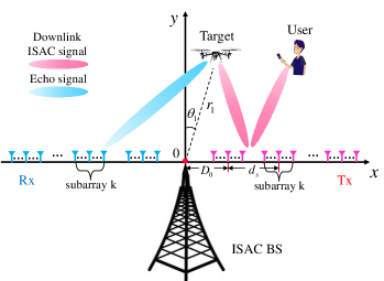
As illustrated in Fig. 1, we consider a downlink ISAC system, where the ISAC BS equipped with modular XL-arrays communicates with a multi-antenna user while simultaneously sensing a radar target. To suppress leakage signals from transmitter and receive the clear sensing echoes, the BS is assumed to be equipped with two spatially widely separated XL-arrays. The total number of transmit and receive antennas is $N=KM$, with $K$ being the number of subarrays and $M$ being the number of antenna elements within each subarray. The communication user has $N_{c}$ antennas, with $N_{c}\ll N$.

The antenna spacing within each subarray is $d=\frac{\lambda}{2}$, where $\lambda$ is the wavelength. For each subarray, we select its center element as the reference antenna. We denote the inter-subarray spacing $d_{s}=\Gamma d$ as the distance between the reference antennas of the adjacent subarrays, where $\Gamma\geq M$. There are two main reasons for considering $d_{s}$ to be much larger than $Md$. Firstly, this is necessary to accommodate practical mounting structures, such as modular XL-arrays mounted on building facades that are separated by windows. Secondly, a large inter-subarray spacing can result in an expanded array aperture, denoted by $S$, which in turn increases the near-field range of the overall antenna array, i.e., $\frac{2S^{2}}{\lambda}$. This expansion enables user who was initially located in the far field of a collocated array to now be within the near-field range of the modular array, thereby allowing them to benefit from various advantages.

The transmit and receive XL-arrays of the BS are placed along the $x$-axis, symmetrically centered around the origin. Due to the wide separation of the receive and transmit arrays, we denote the distance from the reference antenna of the first subarray to the origin as $D_{0}$. Thus, the position of $m$-th array element of $k$-th subarray at Tx, where $m\in\mathcal{M}\triangleq\{1,2,\ldots,M\}$ and $k\in\mathcal{K}\triangleq\{1,2,\ldots,K\}$, can be represented as $\mathbf{l}_{k,m}^{t}=({x}_{k,m}^{t},0)$, with ${x}_{k,m}^{t}=D_{0}+(k-1)d_{s}+(m-1)d$. Similarly, the position of $m$-th array element of $k$-th subarray at Rx is $\mathbf{l}_{k,m}^{r}=({x}_{k,m}^{r},0)$, where ${x}_{k,m}^{r}=-D_{0}-(k-1)d_{s}-(m-1)d$. Suppose that a user, target, scatterer or interference is located at $\mathbf{l}_{q}=(r\sin\theta,r\cos\theta)$, where $r$ is its distance from the origin, and $\theta\in\left[-\frac{\pi}{2},\frac{\pi}{2}\right]$ is its angle with respect to the positive $y$-axis.

Refer to caption
Figure 1: Illustration of the downlink ISAC scenario where the BS equipped with modular XL-arrays serves a multi-antenna communication user while sensing a target.

II-A Near Field HPSW Model for Modular XL-array

Based on the relationship between $r$ and the Rayleigh distance $\frac{2S^{2}}{\lambda}$, the space can be roughly partitioned into three parts, each corresponding to a specific model, namely, the planar-wave model (PWM), spherical-wave model (SWM), and HSPM, as elaborated below.

II-A1 Conventional PWM

When $r\geq\frac{2S^{2}}{\lambda}$, the user, target, scatterer or interference is located in the far-field region of the entire array at the Tx/Rx of the BS. In this case, the PWM is suitable for far-field propagation region, where the transmit and receive array response vectors of the BS can be respectively denoted as:

$\displaystyle\mathbf{a}_{t}^{\text{PWM}}\left(\theta\right)={{\left[{{e}^{-j\frac{2\pi}{\lambda}\varphi_{k,m}^{t}}}\right]}_{\forall k\in\mathcal{K},\forall m\in\mathcal{M}}^{T}},$ (1)
$\displaystyle\mathbf{a}_{r}^{\text{PWM}}\left(\theta\right)={{\left[{{e}^{-j\frac{2\pi}{\lambda}\varphi_{k,m}^{r}}}\right]}_{\forall k\in\mathcal{K},\forall m\in\mathcal{M}}^{T}},$

where $\varphi_{k,m}^{t}=x_{k,m}^{t}sin\theta$ and $\varphi_{k,m}^{r}=x_{k,m}^{r}sin\theta$ denote the virtual angles.

II-A2 Accurate SWM

When $r\leq\frac{2(M-1)^{2}d^{2}}{\lambda}$, the user/target/scatter is not only situated in the near-field region of the entire antenna array, but also within the near-field region of each sub-array. Consequently, the accurate SWM is applicable, leveraging the exact distances between $\mathbf{l}_{q}$ and each array element at Tx/Rx. The distances between $\mathbf{l}_{q}$ and the $m$-th array element in $k$-th subarray at Tx and Rx are respectively expressed as

$\displaystyle r_{k,m}^{t}=\left\|\mathbf{l}_{q}-\mathbf{l}_{k,m}^{t}\right\|=\sqrt{r^{2}-2r({x}_{k,m}^{t})\sin\theta+({x}_{k,m}^{t})^{2}},$ (2)
$\displaystyle r_{k,m}^{r}=\left\|\mathbf{l}_{q}-\mathbf{l}_{k,m}^{r}\right\|=\sqrt{r^{2}-2r({x}_{k,m}^{r})\sin\theta+({x}_{k,m}^{r})^{2}}.$

Therefore, the array response vectors at Tx and Rx for $\mathbf{l}_{q}$ are respectively given by[11, 10]

$\displaystyle\mathbf{a}_{t}^{\text{SWM}}\left(\theta\right)={{\left[{{e}^{-j\frac{2\pi}{\lambda}r_{k,m}^{t}}}\right]}_{\forall k\in\mathcal{K},\forall m\in\mathcal{M}}^{T}},$ (3)
$\displaystyle\mathbf{a}_{r}^{\text{SWM}}\left(\theta\right)={{\left[{{e}^{-j\frac{2\pi}{\lambda}r_{k,m}^{r}}}\right]}_{\forall k\in\mathcal{K},\forall m\in\mathcal{M}}^{T}}.$

II-A3 Harmonic HSPM

When $\frac{2(M-1)^{2}d^{2}}{\lambda}<r<\frac{2S^{2}}{\lambda}$, on one hand, SWM needs to be considered among subarrays due to $r<\frac{2S^{2}}{\lambda}$; on the other hand, PWM needs to be considered within a subarray due to $r>\frac{2(M-1)^{2}d^{2}}{\lambda}$. As such, the HSPM, combining spherical wave propagation between subarrays and plane wave propagation within subarrays is applicable. In contrast to existing research that employs uniform HSPM for common angle of arrival (AoA)s/ angle of departure (AoD)s[10], we consider the spherical wavefronts with phase variation across subarrays, and utilize HSPM for distinct AoAs/AoDs. Specifically, by representing the position of the $k$-th subarray using the location of the reference antenna in the $k$-th subarray, i.e., $\mathbf{l}_{k}^{t}=\mathbf{l}_{k,1}^{t}$ and $\mathbf{l}_{k}^{r}=\mathbf{l}_{k,1}^{r}$, the Tx and Rx array response vectors can be obtained as

$\displaystyle\mathbf{a}_{t}\!^{\text{HSPM}}\!\!\left(r,\theta\right)={{\left[{{e}\!^{-j\frac{2\pi}{\lambda}\left\|{{\mathbf{l}}_{q}}-\mathbf{l}_{k}^{t}\right\|}}{{e}^{-j\frac{2\pi}{\lambda}(m-1)d\sin\theta_{k}^{t}}}\right]}_{\forall k\in\mathcal{K},\forall m\in\mathcal{M}}^{T}},$ (4)
$\displaystyle\mathbf{a}_{r}\!^{\text{HSPM}}\!\!\left(r,\theta\right)={{\left[{{{e}\!^{-j\frac{2\pi}{\lambda}\left\|{{\mathbf{l}}_{q}}-\mathbf{l}_{k}^{r}\right\|}}}{{e}^{-j\frac{2\pi}{\lambda}(m-1)d\sin\theta_{k}^{r}}}\right]}_{\forall k\in\mathcal{K},\forall m\in\mathcal{M}}^{T}},$

where ${\theta}_{k}^{t}$ and ${\theta}_{k}^{r}$ are the angles of $\mathbf{l}_{q}$ as observed from the $k$-th subarray at Tx and Rx. Following Fig. 1, we have

$\displaystyle\sin\theta_{k}^{t}=\frac{r\sin\theta-{{D}_{0}}-\left(k-1\right){{d}_{s}}}{\left\|{{\mathbf{l}}_{q}}-\mathbf{l}_{k}^{t}\right\|},$ (5)
$\displaystyle\sin\theta_{k}^{r}=\frac{r\sin\theta+{{D}_{0}}+\left(k-1\right){{d}_{s}}}{\left\|{{\mathbf{l}}_{q}}-\mathbf{l}_{k}^{r}\right\|}.$

In conclusion, SWM accurately captures the signal amplitude and phase variations of all array elements, making it the most accurate and generic model. However, it is associated with high complexity in modeling and signal processing. The PWM serves as an approximation of the SWM when the array aperture $S$ is significantly smaller than the distance $r$. However, the approximation error of the PWM grows as the array aperture increases[16]. Therefore, in the considered modular XL-MIMO architecture, PWM becomes inaccurate. By comparison, HSPM outperforms PWM in terms of accuracy and exhibits lower complexity compared to SWM, making it a more tractable and accurate near-field array model[17, 10].

II-B Transmit ISAC Signal

Due to the extremely large number of antennas in XL-MIMO systems, the implementation cost of a fully digital beamforming architecture is unaffordable. Therefore, we consider a modular XL-MIMO hybrid digital and analog architecture, where $M_{{\text{RF}}}$ RF chains are assigned to control one subarray. The total number of RF chains at Tx is $N_{\text{RF}}=KM_{\text{RF}}$. Additionally, due to the multiple antennas deployed at the communication user, the transmission of multiple data streams $N_{s}$ for a single user can be realized, where $N_{s}\leq N_{\text{RF}}$.

In particular, we consider a coherent time block consisting of $L$ symbols, during which the communication channels and sensing target parameters are assumed to remain invariant. Let $\mathbf{X}\triangleq[\mathbf{x}[1],\mathbf{x}[2],\ldots,\mathbf{x}[L]]\in\mathbb{C}^{N\times L}$ denote the narrowband transmitted ISAC signal, where $\mathbf{x}[l]$ is the transmitted signal at time index $l$. Let $\mathbf{S}=[\mathbf{s}[1],\mathbf{s}[2],\ldots,\mathbf{s}[L]]\in{\mathbb{C}}^{N_{s}\times L}$ denote the information symbol matrix, where $\mathbf{s}[l]$ is the symbol vector transmitted at time index $l$, and $N_{s}$ is the number of data streams. Therefore, the discrete-time transmitted signal at time index $l$ is given by

$$\mathbf{x}[l]={\mathbf{W}}_{\text{RF}}{\mathbf{W}}_{\text{BB}}\mathbf{s}[l],$$ (6)

where $\mathbf{W}_{\text{RF}}\in\mathbb{C}^{N\times N_{\text{RF}}}$ and ${{\mathbf{W}}_{\text{BB}}}\text{=}\left[{{\mathbf{w}}_{\text{BB},1}},\ldots,{{\mathbf{w}}_{\text{BB},{{N}_{s}}}}\right]\in{{\mathbb{C}}^{{{N}_{\text{RF}}}\times{{N}_{s}}}}$ denote the analog and digital beamformers, respectively. Each entry in $\mathbf{S}$ is assumed to be i.i.d. and Gaussian distributed with zero mean and unit variance. The data streams are assumed to be independent of each other, so we have $\mathbb{E}\left\{\mathbf{s}[l]\mathbf{s}^{H}[l]\right\}=\mathbf{I},\forall l$[5]. Then, the covariance matrix of transmitted signal can be given by

$$\mathbf{R}_{X}=\mathbb{E}\left\{\mathbf{x}[l]\mathbf{x}^{H}[l]\right\}={{\mathbf{W}}_{\text{RF}}}{{\mathbf{W}}_{\text{BB}}}\mathbf{W}_{\text{BB}}^{H}\mathbf{W}_{\text{RF}}^{H}.$$ (7)

Moreover, owing to the hardware limitations of modular XL-MIMO, the RF chains that are connected to one subarray cannot be connected to other subarrays, leading to a partially connected HBF architecture[8]. The analog beamformer ${{\mathbf{W}}_{\text{RF}}}$ holds the block diagonal structure, which is expressed as

$${{\mathbf{W}}_{\text{RF}}}=\mathrm{diag}\left(\mathbf{\tilde{W}}_{\text{RF}}^{1},\cdots,\mathbf{\tilde{W}}_{\text{RF}}^{K}\right),$$ (8)

where $\mathbf{\tilde{W}}_{\text{RF}}^{k}=\left[{{\mathbf{w}}_{k1}},{{\mathbf{w}}_{k2}},\ldots,{{\mathbf{w}}_{k{{M}_{\text{RF}}}}}\right]\in\mathbb{C}^{M\times M_{\text{RF}}}$ is the analog beamformer of the $k$-th subarray, ${{\mathbf{w}}_{kt}}$, $\forall t=1,2,\cdots,M_{\text{RF}}$ are the values of the phase shifters at the $k$-th subarray, and each element in ${{\mathbf{w}}_{kt}}$ has unit modulus and continuous phase, i.e., $\left|\mathbf{w}_{kt}[m]\right|^{2}=1,\forall m\in\mathcal{M}$. Additionally, the normalized transmit power constraint is given by $\left\|\mathbf{W}_{\text{RF}}\mathbf{W}_{\text{BB}}\right\|_{F}^{2}\leq N_{s}$.

III Performance Metrics and Problem Formulation

III-A Communication Performance

As the size of the user’s antenna array is considerably smaller than the transmit XL-array at the BS, i.e., $N_{c}\ll N$, the communication channel between the transmit subarrays and the user’s small receive array can be assumed to exhibit the plane wavefront. On the other hand, due to the large aperture of the transmit antenna array, the spherical-wave propagation needs to be considered among the subarrays.

The planar-wave channel matrix between the $k$-th transmit subarray and the user can be written as[18, 8]:

$$\mathbf{H}_{\text{sub}}^{k}=\sum\limits_{p=1}^{{{N}_{p}}}{\mu_{p}^{k}}\mathbf{a}_{cp}^{k}\left(\theta_{cp}^{k}\right)\mathbf{a}_{tp}^{k}{{\left(\theta_{tp}^{k}\right)}^{H}},$$ (9)

where ${\mu_{p}^{k}}=\left|\mu_{p}^{k}\right|{{e}^{-j\frac{2\pi}{\lambda}D_{p}^{k}}}$ denotes the complex gain of $p$-th path between the reference antennas of the $k$-th transmit subarray and the user’s receive array, $D_{p}^{k}$ represents the distance between the $k$-th reference antenna and the received reference antenna along the $p$-th multipath, with $p=1$ and $p>1$ representing the line-of-sight (LoS) path and the NLoS path, respectively. $\theta_{cp}^{k}$ and $\theta_{tp}^{k}$ represent the AoA and AoD pairs for the $p$-th path between the $k$-th transmit subarray and the user’s receive array. The array steering vector of the $p$-th path for the $k$-th transmit subarray is denoted as $\mathbf{a}_{tp}^{k}\left(\theta_{tp}^{k}\right)={{\left[1,{{e}^{-j\frac{2\pi}{\lambda}d\sin\theta_{tp}^{k}}},\ldots,{{e}^{-j\frac{2\pi}{\lambda}(M-1)d\sin\theta_{tp}^{k}}}\right]}^{T}}$. Similarly, the array steering vector of the $p$-th path for the user’s receive array is denoted as $\mathbf{a}_{cp}^{k}\left(\theta_{cp}^{k}\right)={{\left[1,{{e}^{-j\frac{2\pi}{\lambda}d\sin\theta_{cp}^{k}}},\ldots,{{e}^{-j\frac{2\pi}{\lambda}({{N}_{c}}-1)d\sin\theta_{cp}^{k}}}\right]}^{T}}$.

Therefore, based on HSPM, the communication channel for single-user multi-stream transmission is given by (10), shown at the top of the page.

$\displaystyle{{\mathbf{H}}_{c}}=\left[\begin{matrix}\mathbf{H}_{\text{sub}}^{1}&\cdots&\mathbf{H}_{\text{sub}}^{K}\\ \end{matrix}\right]=\left[\begin{matrix}\sum\limits_{p=1}^{{{N}_{p}}}{\mu_{p}^{1}}\left[\mathbf{a}_{cp}^{1}\left(\theta_{cp}^{1}\right)\mathbf{a}_{tp}^{1}{{\left(\theta_{tp}^{1}\right)}^{H}}\right]&\cdots&\sum\limits_{p=1}^{{{N}_{p}}}{\mu_{p}^{K}}\left[\mathbf{a}_{cp}^{K}\left(\theta_{cp}^{K}\right)\mathbf{a}_{tp}^{K}{{\left(\theta_{tp}^{K}\right)}^{H}}\right]\end{matrix}\right].$ (10)


In the mmWave/sub-THz band, the channels tend to be more sparse due to significant losses caused by large reflection, diffraction, and scattering effects [19, 20]. As paths with insignificant path gains can be disregarded, the number of multipaths in the mmWave/sub-THz band is quite limited. This limitation can decrease the rank of the communication channel, leading to a decline in the communication spectral efficiency. By making the assumption $KN_{p}\leq N_{c}<N$, we conduct an analysis of the rank of ${{\mathbf{H}}_{c}}$ in Lemma 1 below.

Lemma 1

The rank of ${{\mathbf{H}}_{c}}$ satisfies

$$\mathrm{rank}\left({{\mathbf{H}}_{c}}\right)=KN_{p}.$$ (11)
Proof:

Firstly, for a given propagation path $p$, the subarray response vectors $\mathbf{a}_{tp}^{1}\left(\theta_{tp}^{1}\right),\ldots,\mathbf{a}_{tp}^{K}\left(\theta_{tp}^{K}\right)$ are linearly independent[16]. Furthermore, due to the distinguishability of propagation paths and their varying angles, the response vectors associated with different propagation paths $\mathbf{a}_{t1}^{k}\left(\theta_{t1}^{k}\right),\ldots,\mathbf{a}_{tN_{p}}^{k}(\theta_{tN_{p}}^{k})$ are linearly independent for the $k$-th subarray. Therefore, we can obtain that each row of the communication channel $\mathbf{H}_{c}$ in (10) is a linear combination of $KN_{p}$ linearly independent vectors as

$$\mathbf{\bar{a}}_{tp}^{k}{{\left(\phi_{tp}^{k}\right)}^{T}}\triangleq\left[\underbrace{{0},\ldots,{0}}_{k-1},\mathbf{a}_{tp}^{k}{{\left(\phi_{tp}^{k}\right)}^{T}},\underbrace{{0},\ldots,{0}}_{K-k}\right]^{T},$$ (12)

where $k=1,2,\cdots,K$, $p=1,2,\cdots,N_{p}$. ∎

This demonstrates that compared to the traditional far-field PWM channel whose rank is upper-bounded by the number of multipaths $N_{p}$[21], the subarray-based near-field HSPM channel possesses a more sufficient rank, thus enabling it to provide more spatial multiplexing gains.

Given the transmit signal in (6), the received signal of the user is expressed as

$${{\mathbf{Y}}_{c}}={{\mathbf{H}}_{c}}\mathbf{X}+{{\mathbf{Z}}_{c}}={{\mathbf{H}}_{c}}{{\mathbf{W}}_{\text{RF}}}{{\mathbf{W}}_{\text{BB}}}\mathbf{S}+{{\mathbf{Z}}_{c}},$$ (13)

where ${{\mathbf{Z}}_{c}}\in\mathbb{C}^{N_{c}\times L}$ is a zero-mean complex Gaussian noise matrix with covariance matrix $\sigma_{c}^{2}\mathbf{I}_{N_{c}}$. Then, the achievable communication spectral efficiency can be calculated as[22]

$$C=\log\det\left(\mathbf{I}+\frac{1}{\sigma_{c}^{2}}{{\mathbf{H}}_{c}}{{\mathbf{W}}_{\text{RF}}}{{\mathbf{W}}_{\text{BB}}}\mathbf{W}_{\text{BB}}^{H}\mathbf{W}_{\text{RF}}^{H}\mathbf{H}_{c}^{H}\right).$$ (14)

III-B Sensing Performance

For radar sensing, we assume that the BS detects the target of interest located at $\mathbf{l}_{1}=(r_{1}\sin{\phi}_{1},r_{1}\cos{\phi}_{1})$. Assuming there exist $Q-1$ signal-dependent uncorrelated interferences located at $\mathbf{l}_{q}=(r_{q}\sin{\phi}_{q},r_{q}\cos{\phi}_{q}),\forall q\in\{2,3,\cdots,Q\}$, the received signal at the BS over $L$ symbols can be written as

$${{\mathbf{Y}}_{s}}=\underbrace{{{\beta}_{{1}}}{{\mathbf{g}}_{r1}}\mathbf{g}_{t1}^{H}\mathbf{X}}_{\text{Target reflection}}+\underbrace{\sum\nolimits_{q=2}^{Q}{{{\beta}_{q}}{{\mathbf{g}}_{rq}}\mathbf{g}_{tq}^{H}\mathbf{X}}}_{\text{Echo signal of interferences}}+{{\mathbf{Z}}_{s}}$$ (15)

where $\beta_{q}$ is the complex reflection coefficient proportional to the radar cross section (RCS) of the $q$-th object with $\mathbb{E}\left\{\left|\beta_{q}\right|^{2}\right\}=\alpha_{q}^{2}$ ($q=1$ for the target and $q\neq 1$ for the interferences), and ${{\mathbf{Z}}_{s}}=\left[{{\mathbf{z}}_{1}},{{\mathbf{z}}_{2}},\ldots,{{\mathbf{z}}_{L}}\right]\in{{\mathbb{C}}^{N\times L}}$ denotes the additive white Gaussian noise (AWGN), with each column being independent and i.i.d. circularly symmetric complex Gaussian random vector with zero mean and covariance $\mathbf{R}_{s}=\sigma_{s}^{2}\mathbf{I}_{N}$. Additionally, ${{\mathbf{g}}_{rq}}$ and ${{\mathbf{g}}_{tq}}$ denote the receive and transmit array response vectors for the $q$-th object at BS based on HSPM, respectively, which can be expressed as

$\displaystyle{{\mathbf{g}}_{tq}}={{\mathbf{g}}_{t}}\left({{\mathbf{l}}_{q}}\right)=\left(\mathrm{diag}\left({{\bm{\nu}}_{tq}}\right)\otimes{{\mathbf{I}}_{M}}\right){{{\mathbf{\hat{a}}}}_{tq}},$ (16)
$\displaystyle{{\mathbf{g}}_{rq}}={{\mathbf{g}}_{r}}\left({{\mathbf{l}}_{q}}\right)=\left(\mathrm{diag}\left({\bm{\nu}_{rq}}\right)\otimes{{\mathbf{I}}_{M}}\right){{{\mathbf{\hat{a}}}}_{rq}},\forall q\in\{1,\cdots,Q\},$

where ${{\mathbf{\hat{a}}}_{tq}}={{[{{(\mathbf{a}_{tq}^{1})}^{T}},{{(\mathbf{a}_{tq}^{2})}^{T}},\ldots,{{(\mathbf{a}_{tq}^{K})}^{T}}]}^{T}}$ and ${{\mathbf{\hat{a}}}_{rq}}={{[{{(\mathbf{a}_{rq}^{1})}^{T}},{{(\mathbf{a}_{rq}^{2})}^{T}},\ldots,{{(\mathbf{a}_{rq}^{K})}^{T}}]}^{T}}$, with $\mathbf{a}_{tq}^{k}={{[1,{{e}^{-j\frac{2\pi}{\lambda}d\sin\phi_{tq}^{k}}},\ldots,{{e}^{-j\frac{2\pi}{\lambda}(M-1)d\sin\phi_{tq}^{k}}}]}^{T}}$ and $\mathbf{a}_{rq}^{k}={{[1,{{e}^{-j\frac{2\pi}{\lambda}d\sin\phi_{rq}^{k}}},\ldots,{{e}^{-j\frac{2\pi}{\lambda}(M-1)d\sin\phi_{rq}^{k}}}]}^{T}}$ denoting the intra-subarray response vectors for the Tx and Rx under the uniform planar-wave assumption, respectively. The angles of $\mathbf{l}_{q}$ as observed from the $k$-th subarray at Tx and Rx are denoted as ${\phi}_{tq}^{k}$ and ${\phi}_{rq}^{k}$, respectively, which can be obtained as

$\displaystyle\sin\phi_{tq}^{k}=\frac{r_{q}\sin\phi_{q}-{{D}_{0}}-\left(k-1\right){{d}_{s}}}{\left\|{{\mathbf{l}}_{q}}-\mathbf{l}_{k}^{t}\right\|},$ (17)
$\displaystyle\sin\phi_{rq}^{k}=\frac{r_{q}\sin\phi_{q}+{{D}_{0}}+\left(k-1\right){{d}_{s}}}{\left\|{{\mathbf{l}}_{q}}-\mathbf{l}_{k}^{r}\right\|}.$

Additionally, ${{\bm{\nu}}_{tq}}$ and ${{\bm{\nu}}_{rq}}$ represent the inter-subarray response vectors of Tx and Rx toward the $q$-th object, respectively, and can be expressed as

$\displaystyle{\bm{\nu}}_{tq}=\left[{e^{-j\frac{2\pi}{\lambda}\left\|{{\mathbf{l}}_{q}}-\mathbf{l}_{1}^{t}\right\|}},\ldots,{{}e^{-j\frac{2\pi}{\lambda}\left\|{{\mathbf{l}}_{q}}-\mathbf{l}_{K}^{t}\right\|}}\right]^{T},$ (18)
$\displaystyle{\bm{\nu}}_{rq}=\left[{{e}^{-j\frac{2\pi}{\lambda}\left\|{{\mathbf{l}}_{q}}-\mathbf{l}_{1}^{r}\right\|}},\ldots,{{e}^{-j\frac{2\pi}{\lambda}\left\|{{\mathbf{l}}_{q}}-\mathbf{l}_{K}^{r}\right\|}}\right]^{T}.$

Then, the received signal for the probing target is filtered by the receive beamformer $\mathbf{w}\in\mathbb{C}^{N\times 1}$, and the output of the BS receiver is given as

$\displaystyle{\mathbf{y}_{s}}={{\mathbf{w}}^{H}}{{\beta}_{1}}{{\mathbf{g}}_{r1}}\mathbf{g}_{t1}^{H}\mathbf{X}+{{\mathbf{w}}^{H}}\sum\nolimits_{q=2}^{Q}{{{\beta}_{q}}{{\mathbf{g}}_{rq}}\mathbf{g}_{tq}^{H}\mathbf{X}}+{{\mathbf{w}}^{H}}{{\mathbf{Z}}_{s}}.$ (19)

Subsequently, the radar SCNR can be calculated as [23]

$\displaystyle{\gamma}_{s}$ $\displaystyle=\frac{E\left[{{\left\|{{\mathbf{w}}^{H}}{{\beta}_{\text{1}}}{{\mathbf{g}}_{r1}}\mathbf{g}_{t1}^{H}\mathbf{X}\right\|}^{2}}\right]}{E\left[{{\left\|{{\mathbf{w}}^{H}}\sum\nolimits_{q=2}^{Q}{{{\beta}_{q}}{{\mathbf{g}}_{rq}}\mathbf{g}_{tq}^{H}\mathbf{X}}\right\|}^{2}}\right]+E\left[{{\left\|{{\mathbf{w}}^{H}}{{\mathbf{Z}}_{s}}\right\|}^{2}}\right]}$ (20)
$\displaystyle=\frac{\alpha_{1}^{2}{{\mathbf{w}}^{H}}{{\mathbf{g}}_{r1}}\mathbf{g}_{t1}^{H}{{\mathbf{R}}_{X}}{{\mathbf{g}}_{t1}}\mathbf{g}_{r1}^{H}\mathbf{w}}{{{\mathbf{w}}^{H}}\left(\sum\nolimits_{q=2}^{Q}{\alpha_{q}^{2}{{\mathbf{g}}_{rq}}\mathbf{g}_{tq}^{H}{{\mathbf{R}}_{X}}{{\mathbf{g}}_{tq}}\mathbf{g}_{rq}^{H}}+\sigma_{s}^{2}{{\mathbf{I}}_{N}}\right)\mathbf{w}}.$

When $\mathbf{R}_{X}$ is given, the optimal $\mathbf{w}^{*}$ to maximize the SCNR can be derived by solving the equivalent minimum variance distortionless response (MVDR) problem[24], where the closed-form optimal solution can be obtained as

$${\mathbf{w}^{*}}=\frac{{{\left(\bm{\Sigma}+\sigma_{s}^{2}{{\mathbf{I}}_{N}}\right)}^{-1}}{{\mathbf{g}}_{r1}}}{\mathbf{g}_{r1}^{H}{{\left(\bm{\Sigma}+\sigma_{s}^{2}{{\mathbf{I}}_{N}}\right)}^{-1}}{{\mathbf{g}}_{r1}}},$$ (21)

where $\bm{\Sigma}\triangleq\sum\nolimits_{q=2}^{Q}{\alpha_{q}^{2}{{\mathbf{g}}_{rq}}\mathbf{g}_{tq}^{H}{{\mathbf{R}}_{X}}{{\mathbf{g}}_{tq}}\mathbf{g}_{rq}^{H}}$. It is worth noting that once the optimal transmit covariance matrix $\mathbf{R}_{X}$ is derived, the optimal receive beamformer ${\mathbf{w}^{*}}$ can be readily obtained as a closed-form solution from (21). Therefore, we focus on the optimization of transmit beamforming while adopting a fixed receive beamformer $\mathbf{w}$ to avoid the more complex joint transmit-receive beamforming design.

III-C Problem Formulation

In this paper, we jointly design the analog beamformer $\mathbf{W}_{\text{RF}}$ and digital beamformer $\mathbf{W}_{\text{BB}}$ in order to maximize the achievable communication spectral efficiency while satisfying the constraints imposed by the transmit power budget and sensing SCNR. Based on (14) and (20), the optimization problem can be given by

$\displaystyle\max\limits_{{{\mathbf{W}}_{\text{BB}}},{{\mathbf{W}}_{\text{RF}}}}$ $\displaystyle\ \ \ C$ (22a)
$\displaystyle{\rm s.t.}$ $\displaystyle\ \ \left\|{{\mathbf{W}}_{\text{RF}}}{{\mathbf{W}}_{\text{BB}}}\right\|_{F}^{2}\leq{{N}_{s}},$ (22b)
$\displaystyle\ \ {{\mathbf{W}}_{\text{RF}}}\in{{\mathcal{A}}_{F}},$ (22c)
$\displaystyle\ \ {{\gamma}_{s}}\geq{{\Gamma}_{s}},$ (22d)

where ${{\mathcal{A}}_{F}}$ is the set of block matrices, where each block is an $M\times M_{\text{RF}}$ dimension matrix with constant-magnitude entries. However, due to the specific block-diagonal structure of the analog beamformer in ${\mathcal{A}}_{F}$, this type of joint analog-digital optimization problem is often intractable, leading to the attainment of suboptimal solutions rather than a global optimal solution[15].

IV Low-Complexity Hybrid Beamforming Design

IV-A The Optimal Waveform Covariance Matrix

Before gaining an insight into the solution of the joint analog-digital beamforming optimization problem (22), we first introduce the optimal transmit covariance matrix $\mathbf{R}_{X}^{*}$ for achieving the maximum communication spectral efficiency under the sensing SCNR and transmit power constraints:

$\displaystyle\mathbf{R}_{X}^{*}=$ $\displaystyle\max\limits_{\mathbf{R}_{X}}\ \ \ C$ (23)
$\displaystyle{\rm s.t.}$ $\displaystyle\text{tr}\left({\mathbf{R}_{X}}\right)\leq{{N}_{s}},\ \ {{\mathbf{R}}_{X}}\succeq 0,\ \ {{\gamma}_{s}}\geq{{\Gamma}_{s}}.$

Building upon this, the method for designing the optimal analog and digital beamformers is proposed in the subsequent subsection.

To provide an optimal solutions to the problem (23), we propose to exploit the structure of the communication channel and sensing array response vectors based on HSPM, respectively. Namely, we leverage the following observations:

IV-A1 Structure of the communication channel based on HSPM

We begin by performing the singular-value-decomposition (SVD) of the communication channel ${{\mathbf{H}}_{c}}={{\mathbf{U}}_{c}}{{\mathbf{\Sigma}}_{c}}{{\mathbf{V}}_{c}}^{H}$, where ${\mathbf{U}}_{c}\in\mathbb{C}^{N_{c}\times KN_{p}}$ and ${\mathbf{V}}_{c}\in\mathbb{C}^{N\times KN_{p}}$ are unitary matrices, and ${{\mathbf{\Sigma}}_{c}}\in\mathbb{C}^{KN_{p}\times KN_{p}}$ is a diagonal matrix of singular values arranged in decreasing order. The columns of the unitary matrix ${\mathbf{V}}_{c}$ form an orthonormal basis for the ${\mathbf{H}}_{c}$’s row space. Besides, according to Lemma 1 and its proof, we note that the $KN_{p}$ linearly independent vectors $\tilde{\mathbf{a}}_{tp}^{k}\left(\theta_{tp}^{k}\right),\forall k,p$ form another minimal basis for the $\mathbf{H}_{c}$’s row space. Therefore, the columns of ${\mathbf{V}}_{c}$ can be written as linear combinations of $\tilde{\mathbf{a}}_{tp}^{k}\left(\theta_{tp}^{k}\right),\forall k,p$, i.e.,

$${{\mathbf{V}}_{c}}=\mathbf{\tilde{A}}_{c}\mathbf{T},$$ (24)

where $\mathbf{T}\in\mathbb{C}^{KN_{p}\times KN_{p}}$ represents the linear transformation matrix, and $\mathbf{\tilde{A}}_{c}\in\mathbb{C}^{N\times KN_{p}}$ is a matrix formed by combining $\tilde{\mathbf{a}}_{tp}^{k}\left(\theta_{tp}^{k}\right),\forall k,p$ as column vectors.

IV-A2 Structure of Sensing Array Response Vectors based on HSPM

For a given sensing object $q$, the subarray response vectors $\mathbf{a}_{tq}^{1}(\mathbf{l}_{q}),\ldots,\mathbf{a}_{tq}^{K}(\mathbf{l}_{q})$ are linearly independent because different subarrays observe different AoD of $\mathbf{l}_{q}$. Therefore, each sensing array response vector ${{\mathbf{g}}_{t}}\left({{\mathbf{l}}_{q}}\right)$ can be expressed as a fixed linear combination of $K$ linearly independent vectors as

$$\mathbf{\bar{a}}_{tq}^{k}{{\left(\phi_{tq}^{k}\right)}^{T}}\triangleq\left[\underbrace{{0},\ldots,{0}}_{k-1},\mathbf{a}_{tq}^{k}{{\left(\phi_{tq}^{k}\right)}^{T}},\underbrace{{0},\ldots,{0}}_{K-k}\right],\quad\forall k.$$ (25)

Then, we have the following new representation of the sensing array response vector:

$\displaystyle{{\mathbf{g}}_{t}}\left({{\mathbf{l}}_{q}}\right)={{\mathbf{\bar{A}}}_{tq}}{\bm{\nu}}_{tq},\ \forall q,$ (26)

where

$\displaystyle{{\mathbf{\bar{A}}}_{tq}}=\left[\begin{matrix}\mathbf{\bar{a}}_{tq}^{1}\left(\phi_{tq}^{1}\right),&\mathbf{\bar{a}}_{tq}^{2}\left(\phi_{tq}^{2}\right),&\ldots,&\mathbf{\bar{a}}_{tq}^{K}\left(\phi_{tq}^{K}\right)\\ \end{matrix}\right].$ (27)

IV-A3 Joint Representation of Communication Channel and Sensing Array Response Vectors

To establish the joint representation of the communication channel and sensing array response vectors, we first construct a set consisting of communication and sensing subarray response vectors, which can be given by

$\displaystyle\mathbf{U}=\left[{{{\mathbf{\bar{A}}}}_{t1}},\ldots,{{{\mathbf{\bar{A}}}}_{tQ}},{{{\mathbf{\tilde{A}}}}_{c}}\right]\in{{\mathbb{C}}^{N\times K\left(Q+{{N}_{p}}\right)}}.$ (28)

Then, based on the observations (24) and (26), we can obtain

$${{\mathbf{g}}_{t}}\left({{\mathbf{l}}_{q}}\right)=\mathbf{U}\mathbf{\tilde{{\bm{\nu}}}}_{tq},\ \forall q,$$ (29)
$${{\mathbf{V}}_{c}}=\mathbf{U\tilde{T}},$$ (30)

where

$$\mathbf{\tilde{{\bm{\nu}}}}_{tq}={{\left[\mathbf{0}_{K}^{T},\ldots,{\bm{\nu}}_{tq}^{T},\ldots,\mathbf{0}_{K}^{T}\right]}^{T}}\in{{\mathbb{C}}^{K\left(Q+{{N}_{p}}\right)\times 1}},$$ (31)
$\displaystyle\mathbf{\tilde{T}}$ $\displaystyle=\left[\begin{aligned} &{{\mathbf{0}}_{KQ\times K{{N}_{p}}}}\\ &\mathbf{T}\\ \end{aligned}\right]\in{{\mathbb{C}}^{K\left(Q+{{N}_{p}}\right)\times K{{N}_{p}}}}.$ (32)

Based on the above observations, we can obtain the structure of the optimal transmit covariance matrix for the problem (23), as provided in the theorem below.

Theorem 1

The optimal transmit waveform covariance matrix $\mathbf{R}_{X}^{*}$ can be written in the form as

$$\mathbf{R}_{X}^{*}=\mathbf{\tilde{U}\Lambda}{{\mathbf{\tilde{U}}}^{H}},$$ (33)

where $\mathbf{\Lambda}\in\mathbb{C}^{K(Q+N_{p})\times K(Q+N_{p})}$ is a positive semi-definite matrix, and $\mathbf{\tilde{U}}$ is a block diagonal matrix obtained from $\mathbf{{U}}$ by column permutations, i.e.,

$\displaystyle\mathbf{\tilde{U}}$ $\displaystyle=\mathbf{UP}=\left[\begin{matrix}{{{\mathbf{\tilde{U}}}}_{1}}&\cdots&{{{\mathbf{\tilde{U}}}}_{K}}\\ \end{matrix}\right]$ (34)
$\displaystyle=\left[\begin{matrix}{{\mathbf{A}}_{11}}&\mathbf{0}&\cdots&\mathbf{0}\\ \mathbf{0}&{{\mathbf{A}}_{22}}&\cdots&\mathbf{0}\\ \vdots&\vdots&\ddots&\vdots\\ \mathbf{0}&\mathbf{0}&\cdots&{{\mathbf{A}}_{KK}}\\ \end{matrix}\right],$

where $\mathbf{P}$ is a permutation matrix of size $K(Q+N_{p})$, and $\forall k\in\left\{1,\ldots,K\right\}$ we have

$\displaystyle{{\mathbf{\tilde{U}}}_{k}}\!$ $\displaystyle=\!\left[\mathbf{\bar{a}}_{t1}^{k}\!\left(\phi_{t1}^{k}\right)\!,\ldots,\mathbf{\bar{a}}_{tQ}^{k}\!\left(\!\phi_{tQ}^{k}\!\right)\!,\mathbf{\tilde{a}}_{t1}^{k}\!\left(\theta_{t1}^{k}\right)\!,\ldots,\mathbf{\tilde{a}}_{t{{N}_{p}}}^{k}\!\left(\!\theta_{t{{N}_{p}}}^{k}\!\right)\!\right],$ (35a)
$\displaystyle{{\mathbf{A}}_{kk}}\!$ $\displaystyle=\!\left[\mathbf{a}_{t1}^{k}\!\left(\phi_{t1}^{1}\right)\!,\ldots,\mathbf{a}_{tQ}^{k}\!\left(\phi_{tQ}^{1}\right)\!,\mathbf{a}_{t1}^{k}\!\left(\theta_{t1}^{k}\right)\!,\ldots,\mathbf{a}_{t{{N}_{p}}}^{k}\!\left(\!\theta_{t{{N}_{p}}}^{k}\!\right)\!\right].$ (35b)
Proof:

Please see Appendix A. ∎

Theorem 1 demonstrates that the optimal waveform covariance matrix $\mathbf{R}_{X}^{*}$ belongs to the column space of the block diagonal matrix ${\mathbf{\tilde{U}}}$, which is also the subspace spanned by the communication and sensing subarray response vectors. In the following subsection, we exploit the structure of $\mathbf{R}_{X}^{*}$ to design the optimal analog and digital beamformers for the problem (22).

IV-B Equivalent Low-dimensional Optimization Problem

To fully utilize the multiplexing gain, we have $N_{s}=\mathrm{rank}(\mathbf{H}_{c})=KN_{p}$. In addition, in the mmWave/sub-THz band, where reflection and scattering losses are significant, the contributions of high-order reflection and scattering paths can be neglected, leading to a small value of $N_{p}$. Therefore, in scenarios where the number of subarrays and the number of interferences are limited, we can consider $N_{p}+Q$ to be much smaller than $M$. Consequently, we can use $M_{\text{RF}}=N_{p}+Q$ RF chains at each subarray, and the total number of RF chains is $N_{\text{RF}}=K(N_{p}+Q)$.

Based on the above and Theorem 1, we have the following lemma for obtaining the optimal analog beamformer for problem (22).

Lemma 2

The optimal analog beamformer $\mathbf{W}_{\text{RF}}^{*}$ of problem (22) can be expressed as

$${\mathbf{W}_{\text{RF}}^{*}}=\mathbf{\tilde{U}}.$$ (36)
Proof:

Note that both communication and sensing subarray response vectors in (35b) are constant-magnitude phase-only vectors. Therefore, ${\mathbf{\tilde{U}}}$ satisfies both the diagonal matrix constraint and the constant modulus constraint., i.e., ${\mathbf{\tilde{U}}}\in{{\mathcal{A}}_{F}}$, which indicates that ${\mathbf{\tilde{U}}}$ can be applied as the analog beamformer. It is evident that matrix $\mathbf{W}_{\text{BB}}\mathbf{W}{{{}_{\text{BB}}}^{H}}$ is positive semi-definite, hence ${\mathbf{\tilde{U}}}\mathbf{W}_{\text{BB}}\mathbf{W}{{{}_{\text{BB}}}^{H}}{\mathbf{\tilde{U}}}^{H}$ conforms to the structure of the optimal waveform covariance matrix defined in (33). Therefore, ${\mathbf{\tilde{U}}}$ can be considered as the optimal analog beamformer, which completes the proof. ∎

By substituting (36) into (14) and (20), the achievable communication spectral efficiency and sensing SCNR can be respectively rewritten as

$$C=\log\det\left(\mathbf{I}+\frac{1}{\sigma_{c}^{2}}{{\mathbf{H}}_{c}}\mathbf{\tilde{U}}{{\mathbf{W}}_{\text{BB}}}\mathbf{W}_{\text{BB}}^{H}{{{\mathbf{\tilde{U}}}}^{H}}\mathbf{H}_{c}^{H}\right),$$ (37)
$${{\gamma}_{s}}=\frac{\alpha_{1}^{2}\text{tr}\left({{\mathbf{W}}_{\text{BB}}}\mathbf{W}_{\text{BB}}^{H}{{\mathbf{\Phi}}_{1}}\right)}{\sum\nolimits_{q=2}^{Q}{\alpha_{q}^{2}\text{tr}\left({{\mathbf{W}}_{\text{BB}}}\mathbf{W}_{\text{BB}}^{H}{{\mathbf{\Phi}}_{q}}\right)}+\sigma_{s}^{2}\mathbf{w}{{\mathbf{w}}^{H}}},$$ (38)

where ${{\mathbf{\Phi}}_{q}}\triangleq{{\mathbf{\tilde{U}}}^{H}}{{\mathbf{g}}_{tq}}\mathbf{g}_{rq}^{H}\mathbf{w}{{\mathbf{w}}^{H}}{{\mathbf{g}}_{rq}}\mathbf{g}_{tq}^{H}\mathbf{\tilde{U}}$, $\forall q\in\left\{1,2,\ldots,Q\right\}$. Moreover, due to the block diagonal structure of $\mathbf{{W}}_{\text{RF}}$, each non-zero element of $\mathbf{W}_{\text{RF}}$ is multiplied with the corresponding row in $\mathbf{{W}}_{\text{BB}}$. Hence, the constraint (22b) can be simplified as

$$\left\|{{\mathbf{W}}_{\text{RF}}}{{\mathbf{W}}_{\text{BB}}}\right\|_{F}^{\text{2}}\text{=}M\left\|{{\mathbf{W}}_{\text{BB}}}\right\|_{F}^{\text{2}}\leq N_{s}.$$ (39)

Therefore, the complex joint analog-digital beamforming optimization problem (22) can be equivalently simplified into a low-dimensional digital beamforming optimization problem with the given optimal analog beamformer, i.e.,

$\displaystyle\underset{{{\mathbf{W}}_{\text{BB}}}}{\mathop{\max}}\,$ $\displaystyle\ \ \log\det\left(\mathbf{I}+\frac{1}{\sigma_{c}^{2}}\mathbf{W}_{\text{BB}}^{H}{{{\mathbf{\tilde{U}}}}^{H}}\mathbf{H}_{c}^{H}{{\mathbf{H}}_{c}}\mathbf{\tilde{U}}{{\mathbf{W}}_{\text{BB}}}\right)$ (40a)
$\displaystyle\text{s}.\text{t}.$ $\displaystyle\ \ \text{tr}\left({{\mathbf{W}}_{\text{BB}}}\mathbf{W}_{\text{BB}}^{H}\right)\leq\frac{{{N}_{s}}}{M},$ (40b)
$\displaystyle\begin{split}{}&\ \ \alpha_{1}^{2}\text{tr}\left(\mathbf{W}_{\text{BB}}^{H}{{\mathbf{\Phi}}_{1}}{{\mathbf{W}}_{\text{BB}}}\right)\text{-}{{\Gamma}_{s}}\sum\limits_{q=2}^{Q}{\alpha_{q}^{2}\text{tr}\left(\mathbf{W}_{\text{BB}}^{H}{{\mathbf{\Phi}}_{q}}{{\mathbf{W}}_{\text{BB}}}\right)}\geq{{\Gamma}_{0}},\\[-8.53581pt] \end{split}$ (40c)

where $\Gamma_{0}\triangleq{{\Gamma}_{s}}\sigma_{s}^{2}\mathbf{w}{{\mathbf{w}}^{H}}$.

Althogh the digital beamformer optimization problem (40), has a reduced dimension, it remains non-convex due to the rank constraint imposed by the limited number of data streams. To tackle this non-convex problem, we propose two distinct algorithms in the following subsections: a manifold optimization method that directly optimizes the digital beamformer on the rank-constrained space and an SDR-based method that obtains a near-optimal solution. By investigating these two optimization strategies, we provide a comprehensive framework for solving the rank-constrained digital beamformer design problem.

IV-C Joint Optimization on Riemannian Manifold and Euclidean Space

In this subsection, we first analyze the structure of the optimal solution to problem (40) without relaxing the rank constraint, and obtain the semi-closed-form solution. Based on this, we then develop a Riemannian joint gradient descent algorithm.

Let $\mathbf{B}\triangleq{{\mathbf{\tilde{U}}}^{H}}\mathbf{H}_{c}^{H}{{\mathbf{H}}_{c}}\mathbf{\tilde{U}}$, and it follows that $\mathbf{B}$ is a Hermitian matrix with $\mathrm{rank}(\mathbf{B})=\min\{N_{\text{RF}},KN_{p}\}=N_{s}$. Performing eigendecomposition on $\mathbf{B}$ and retaining only the non-zero eigenvalues and their corresponding eigenvectors, we obtain $\mathbf{B}={{\mathbf{U}}_{B}}{{\mathbf{\Sigma}}_{B}}\mathbf{U}_{B}^{H}$, where ${{\mathbf{U}}_{B}}\in\mathbb{C}^{N_{\text{RF}}\times N_{s}}$, and $\mathbf{\Sigma}_{B}\in\mathbb{C}^{N_{s}\times N_{s}}$. Then, we can obtain the structure of the optimal solution to the problem (40) in the following Lemma.

Lemma 3

The optimal solution to the problem (40) is given as

$$\mathbf{W}_{\text{BB}}^{*}\text{=}{{\mathbf{U}}_{\text{B}}}\mathbf{\Sigma}_{\text{B}}^{-\frac{1}{2}}\mathbf{U}_{\text{B}}^{H}\mathbf{\tilde{V}\tilde{\Sigma}},$$ (41)

where $\mathbf{\tilde{V}}\in\mathbb{C}^{N_{\text{RF}}\times N_{\text{RF}}}$ is an unitary matrix, and $\tilde{\Sigma}$ is a $N_{\text{RF}}\times N_{s}$ rectangular diagonal matrix which is defined as

$$\mathbf{\tilde{\Sigma}}\text{=}\left[\begin{matrix}\mathrm{diag}\left(\mathbf{b}\right)\\ {\mathbf{0}}_{{N_{\mathrm{RF}}}-N_{s},N_{s}}\\ \end{matrix}\right],$$ (42)

with $\bm{b}=[b_{1},b_{2},\ldots,b_{N_{s}}]^{T}$.

Proof:

Please refer to [25, Theorem 1]. ∎

It can be observed that the unitary matrix $\mathbf{\tilde{V}}$ forms a complex Stiefel mainifold $\mathcal{M}_{s}=\{\mathbf{\tilde{V}}\in\mathbb{C}^{N_{\text{RF}}\times N_{\text{RF}}}:\mathbf{\tilde{V}}^{H}\mathbf{\tilde{V}}=\mathbf{I}_{N_{\text{RF}}}\}$. Therefore, the problem (40) can be rewritten as

$\displaystyle\underset{\mathbf{\tilde{V}},\mathbf{b}}{\mathop{\max}}\,$ $\displaystyle\ \ \log\det\left(\mathbf{I}+\mathbf{\tilde{\Sigma}}{{{\mathbf{\tilde{\Sigma}}}}^{H}}\right)$ (43a)
$\displaystyle\text{s}.\text{t}.$ $\displaystyle\ \ \text{tr}\left({{{\mathbf{\tilde{V}}}}^{H}}\mathbf{\tilde{B}\tilde{V}\tilde{\Sigma}}{{{\mathbf{\tilde{\Sigma}}}}^{H}}\right)\leq\frac{{{N}_{s}}}{M},$ (43b)
$\displaystyle\ \ \text{tr}\left({{{\mathbf{\tilde{V}}}}^{H}}\mathbf{\tilde{\Phi}\tilde{V}\tilde{\Sigma}}{{{\mathbf{\tilde{\Sigma}}}}^{H}}\right)\geq{{\Gamma}_{s}}\sigma_{s}^{2}\mathbf{w}{{\mathbf{w}}^{H}},$ (43c)
$\displaystyle\ \ \mathbf{\tilde{V}}\in\mathcal{M}_{s},$ (43d)
$\displaystyle\ \ \mathbf{b}\in\mathbb{R}^{r},$ (43e)

where

$$\mathbf{\tilde{B}}={{\mathbf{U}}_{\text{B}}}\mathbf{\Sigma}_{\text{B}}^{-1}\mathbf{U}_{\text{B}}^{H},$$ (44)
$$\mathbf{\tilde{\Phi}}\triangleq{{\mathbf{U}}_{\text{B}}}\mathbf{\Sigma}_{\text{B}}^{-\frac{1}{2}}\mathbf{U}_{\text{B}}^{H}\left(\alpha_{1}^{2}{{\mathbf{\Phi}}_{1}}-{{\Gamma}_{s}}\sum\nolimits_{q=2}^{Q}{\alpha_{q}^{2}{{\mathbf{\Phi}}_{q}}}\right){{\mathbf{U}}_{\text{B}}}\mathbf{\Sigma}_{\text{B}}^{-\frac{1}{2}}\mathbf{U}_{\text{B}}^{H}.$$ (45)

We then use the barrier method to make the inequality constraints (43b) and (43c) implicit in the objective function (43a). Thus, we have

$\displaystyle f\left(\mathbf{\tilde{V}},\mathbf{b}\right)$ $\displaystyle=-\log\det\left(\mathbf{I}+\mathbf{\tilde{\Sigma}}{{{\mathbf{\tilde{\Sigma}}}}^{H}}\right)$ (46)
$\displaystyle+\phi\left(\frac{{{N}_{s}}}{M}-\text{tr}\left({{{\mathbf{\tilde{V}}}}^{H}}\mathbf{\tilde{B}\tilde{V}\tilde{\Sigma}}{{{\mathbf{\tilde{\Sigma}}}}^{H}}\right)\right)$
$\displaystyle+\phi\left(\text{tr}\left({{{\mathbf{\tilde{V}}}}^{H}}\mathbf{\tilde{\Phi}\tilde{V}\tilde{\Sigma}}{{{\mathbf{\tilde{\Sigma}}}}^{H}}\right)-\Gamma_{0}\right),$

where $\phi(u)$ is the logarithmic barrier function, i.e.,

$$\phi(u)=\begin{cases}-\frac{1}{t}\ln(u),&u>0\\ +\infty,&u\leq 0\end{cases},$$ (47)

with $t$ barrier parameter $t>0$.

Consequently, problem (43) can be simplified to an unconstrained optimization problem shown as below:

$\displaystyle\underset{\mathbf{\tilde{V}},\mathbf{b}}{\mathop{\min}}\,$ $\displaystyle\ \ f\left(\mathbf{\tilde{V}},\mathbf{b}\right)$ (48a)
$\displaystyle\text{s}.\text{t}.$  $\displaystyle\ \ \text{ }\mathbf{\tilde{V}}\in{{\mathcal{M}}_{s}},\ \ \mathbf{b}\in\mathbb{R}^{N_{s}}.$ (48b)

It can be observed that the variables $\mathbf{\tilde{V}}$ and $\mathbf{b}$ are coupled in the objective function. To account for the interaction between these variables, we engage in the simultaneous optimization of both $\mathbf{\tilde{V}}$ and $\mathbf{b}$, enabling coordinated updates to enhance convergence efficiency along a more effective path.

As a first step, we derive the Euclidean gradients of the objective function with respect to $\mathbf{\tilde{V}}$ and $\mathbf{b}$, respectively. The gradient of the objective function $f(\mathbf{\tilde{V}},\mathbf{b})$ with respect to $\mathbf{b}$ is provided in (50) at the top of this page, where $(\cdot)_{1:N_{s},1:N_{s}}$ represents the top-left $N_{s}\times N_{s}$ block of a matrix. Then, the update of $\mathbf{b}$ at the (n)-th iteration on the Euclidean space is

$$\mathbf{b}^{(n+1)}:=\mathbf{b}^{(n)}+\delta_{\mathbf{b}}^{(n)}\nabla_{\mathbf{b}}^{(n)}f,$$ (49)

where the step size $\delta_{\mathbf{b}}^{(n)}$ is determined by line search algorithms, such as the Armijo rule.

$$\nabla_{\mathbf{b}}f=-2\left(\left(\mathbf{I}+\mathbf{{\tilde{\Sigma}}}\mathbf{{{{\tilde{\Sigma}}}}^{H}}\right)^{-1}_{1:N_{s},1:N_{s}}\right)\mathbf{b}+\frac{2}{t}\left(\frac{\mathrm{diag}{{\left({{{\mathbf{\tilde{V}}}}^{H}}\mathbf{\tilde{B}\tilde{V}}\right)}_{1:{{N}_{s}}}}}{\left(\frac{{{N}_{s}}}{M}-\text{tr}\left({{{\mathbf{\tilde{V}}}}^{H}}\mathbf{\tilde{B}\tilde{V}\tilde{\Sigma}}{{{\mathbf{\tilde{\Sigma}}}}^{H}}\right)\right)}-\frac{\mathrm{diag}{{\left({{{\mathbf{\tilde{V}}}}^{H}}\mathbf{\tilde{\Phi}\tilde{V}}\right)}_{1:{{N}_{s}}}}}{\left(\text{tr}\left({{{\mathbf{\tilde{V}}}}^{H}}\mathbf{\tilde{\Phi}\tilde{V}\tilde{\Sigma}}{{{\mathbf{\tilde{\Sigma}}}}^{H}}\right)-{{\Gamma}_{0}}\right)}\right)\mathrm{diag}(\mathbf{b})$$ (50)


The Euclidean gradient of objective function w.r.t. $\mathbf{\tilde{V}}$ is obtained by

$\displaystyle{{\nabla}_{{\mathbf{\tilde{V}}}}}f$ $\displaystyle=\frac{2}{t}\left(\frac{1}{-\text{tr}\left({{{\mathbf{\tilde{V}}}}^{H}}\mathbf{\tilde{B}\tilde{V}\tilde{\Sigma}}{{{\mathbf{\tilde{\Sigma}}}}^{H}}\right)+\frac{{{N}_{s}}}{M}}\mathbf{\tilde{B}\tilde{V}\tilde{\Sigma}}{{{\mathbf{\tilde{\Sigma}}}}^{H}}\right.$ (51)
$\displaystyle-\left.\frac{\mathbf{\tilde{\Phi}\tilde{V}\tilde{\Sigma}}{{{\mathbf{\tilde{\Sigma}}}}^{H}}}{\text{tr}\left({{{\mathbf{\tilde{V}}}}^{H}}\mathbf{\tilde{\Phi}\tilde{V}\tilde{\Sigma}}{{{\mathbf{\tilde{\Sigma}}}}^{H}}\right)-{{\Gamma}_{0}}}\right).$

The tangent space for the complex Stiefel manifold is given by

$$T_{\mathbf{\tilde{V}}}\mathcal{M}_{s}=\{\mathbf{Z}\in\mathbb{C}^{N_{\text{RF}}\times N_{\text{RF}}}:\mathbf{Z}^{H}{\mathbf{\tilde{V}}}+{\mathbf{\tilde{V}}}^{H}\mathbf{Z}=0\}.$$ (52)

For each point $\mathbf{\tilde{V}}\in\mathcal{M}_{s}$, the decent direction $\bm{\Delta}_{\mathbf{\tilde{V}}}$ is defined as the projection of the Euclidean gradient ${{\nabla}_{{\mathbf{\tilde{V}}}}}f$ onto the tangent space, which is obtained by

$\displaystyle\bm{\Delta}_{\mathbf{\tilde{V}}}=\mathbf{\tilde{V}}^{H}{{\nabla}_{{\mathbf{\tilde{V}}}}}f\mathbf{\tilde{V}}-{{\nabla}_{{\mathbf{\tilde{V}}}}}f.$ (53)

Thus, the update of $\mathbf{\tilde{V}}$ at the (n)-th iteration on the tangent space can be given by

$$\mathbf{\bar{V}}^{(n+1)}=\mathbf{\tilde{V}}^{(n)}+{\delta}_{\mathbf{\tilde{V}}}^{(n)}\bm{\Delta}_{\mathbf{\tilde{V}}}^{(n)},$$ (54)

where ${\delta}_{\mathbf{\tilde{V}}}^{(n)}$ is the step size. However, the new updated point $\mathbf{\bar{V}}^{(n+1)}$ may not necessarily lie on the manifold, necessitating the projection onto the Stiefel manifold.

Proposition 1

Let $\mathbf{Z}\in\mathbb{C}^{N_{\text{RF}}\times N_{\text{RF}}}$ be a arbitrary matrix. The projection $\mathcal{P_{M_{s}}}(\mathbf{Z})$ onto the Stiefel manifold is

$$\mathcal{P}_{\mathcal{M}_{s}}(\mathbf{Z})=\arg\min_{\mathbf{Q}\in\mathcal{M}_{s}}\|\mathbf{Z}-\mathbf{Q}\|^{2}.$$ (55)

Additionally, if the SVD of $\mathbf{Z}$ is $\mathbf{Z}=\mathbf{U}_{Z}\mathbf{\Sigma}_{Z}\mathbf{V}_{Z}^{H}$, then $\mathcal{P}_{\mathcal{M}_{s}}(\mathbf{Z})=\mathbf{U}_{Z}\mathbf{V}_{Z}^{H}$.

Proof:

Please refer to [26, Prop. 7]. ∎

Therefore, at the (n)-th iteration on the mainfold ${\mathcal{M}_{s}}$ is given by

$$\mathcal{P}_{\mathcal{M}_{s}}(\mathbf{\bar{V}}^{(n+1)})=\mathcal{P}_{\mathcal{M}_{s}}(\mathbf{\tilde{V}}^{(n)}+{\delta}^{(n)}\bm{\Delta}_{\mathbf{\tilde{V}}^{(n)}}).$$ (56)

According to the above discuss, the main procedures of the Riemannian projected steepest descent algorithm for solving problem (48) over $\mathbf{\tilde{V}}$ are described in Algorithm 1. Upon termination, the algorithm outputs the obtained solution $(\mathbf{\tilde{V}}^{*},\mathbf{b}^{*})$. It is noted that due to the non-convexity of the problem (48), the algorithm converges to a local optimum rather than a global one. Therefore, the local optimal solution to problem (40) is

$$\mathbf{W}_{\text{BB}}^{*}={{\mathbf{U}}_{\text{B}}}\mathbf{\Sigma}_{\text{B}}^{-\frac{1}{2}}\mathbf{U}_{\text{B}}^{H}\mathbf{\tilde{V}^{*}}\mathbf{\tilde{\Sigma}^{*}},$$ (57)

with

$$\mathbf{\tilde{\Sigma}^{*}}=\left[\begin{matrix}\mathrm{diag}\left(\mathbf{b}^{*}\right)\\ {{\mathbf{0}}_{N_{\text{RF}}-N_{s},N_{s}}}\\ \end{matrix}\right].$$ (58)

The computational complexity of Algorithm 1 is dominated by the SVD decomposition of $\mathbf{B}\triangleq\tilde{\mathbf{U}}^{H}\mathbf{H}_{c}^{H}\mathbf{H}_{c}\tilde{\mathbf{U}}$, the calculation of Riemannian and Euclidean gradients, and the Riemannian projection in each iteration. Computing $\mathbf{B}$ has a complexity of $\mathcal{O}(N_{\text{RF}}N_{c}N)$, while the SVD of $\mathbf{B}$ requires $\mathcal{O}(N_{\text{RF}}^{3})$ operations [27]. The gradient calculations involve matrix multiplications and inversions with a total complexity of $\mathcal{O}(N_{\text{RF}}^{3}+N_{\text{RF}}^{2}N_{s}+N_{\text{RF}}{N_{s}}^{2})$. The Riemannian gradient descent update and projection require $\mathcal{O}(N_{\text{RF}}^{2})$ and $\mathcal{O}(N_{\text{RF}}^{3})$ operations, respectively [28]. Thus, the overall complexity of Algorithm 1 is $\mathcal{O}(I(N_{\text{RF}}N_{c}N+N_{\text{RF}}^{3}+N_{\text{RF}}^{2}N_{s}+N_{\text{RF}}{N_{s}}^{2}))$, where $I$ is the number of iterations.

Algorithm 1 Riemannian Joint Gradient Descent Algorithm
1:  Initialize $N_{s}$, $M$, ${\Gamma}_{s}$, $t>0$, the tolerances $\epsilon_{\tilde{\mathbf{V}}}>0$ and $\epsilon_{\mathbf{b}}>0$, the maximum number of iterations $I^{max}$, and choose a feasible $\mathbf{\tilde{V}}^{(0)}\in\mathbb{C}^{N_{\text{RF}}\times N_{\text{RF}}}$ such that $(\mathbf{\tilde{V}}^{(0)})^{H}\mathbf{\tilde{V}}^{(0)}=\mathbf{I}$ and $\mathbf{b}^{(0)}\in\mathbb{R}^{r}$.
2:  Set $n:=0$, compute the Riemannian gradient $\xi_{\mathbf{\tilde{V}}}^{(0)}=\mathbf{\Delta}_{\mathbf{\tilde{V}}}(\mathbf{\tilde{V}}^{(0)},\mathbf{b}^{(0)})$ and the Euclidean gradient $\xi_{\mathbf{b}}^{(0)}=\nabla_{\mathbf{b}}f(\mathbf{\tilde{V}}^{(0)},\mathbf{b}^{(0)})$;
3:  while $n\leq I^{max}$ and $\|\xi_{\mathbf{\tilde{V}}}^{(n)}\|_{F}^{2}\geq\epsilon_{\tilde{\mathbf{V}}}$ or $\|\xi_{\mathbf{b}}^{(n)}\|^{2}\geq\epsilon_{\mathbf{b}}$ do
4:     Choose the stepsizes $\delta_{\mathbf{\tilde{V}}}^{(n)}$ and $\delta_{\mathbf{b}}^{(n)}$ using backtracking line search such that: $f\left(\mathcal{P}_{\mathcal{M}_{s}}(\mathbf{\tilde{V}}^{(n)}+\delta_{\mathbf{\tilde{V}}}^{(n)}\xi_{\mathbf{\tilde{V}}}^{(n)}),\mathbf{b}^{(n)}+\delta_{\mathbf{b}}^{(n)}\xi_{\mathbf{b}}^{(n)}\right)<f(\mathbf{\tilde{V}}^{(n)},\mathbf{b}^{(n)})$
5:     Update $\mathbf{\tilde{V}}^{(n+1)}:=\mathcal{P}_{\mathcal{M}_{s}}(\mathbf{\tilde{V}}^{(n)}+{\delta_{\mathbf{\tilde{V}}}}^{(n)}\xi_{\mathbf{\tilde{V}}}^{(n)})$;
6:     Update $\mathbf{b}^{(n+1)}:=\mathbf{b}^{(n)}+{\delta_{\mathbf{b}}}^{(n)}\xi_{\mathbf{b}}^{(n)}$;
7:     Update $n:=n+1$;
8:     Compute the descent direction $\xi_{\mathbf{\tilde{V}}}^{(n)}$ as $\xi_{\mathbf{\tilde{V}}}^{(n)}=\mathbf{\Delta}_{\mathbf{\tilde{V}}}(\mathbf{\tilde{V}}^{(n)},\mathbf{b}^{(n)})$ according to (53);
9:     Compute the descent direction $\xi_{\mathbf{b}}^{(n)}$ as $\xi_{\mathbf{b}}^{(n)}=\nabla_{\mathbf{b}}f(\mathbf{\tilde{V}}^{(n)},\mathbf{b}^{(n)})$ according to (50);
10:  end while
11:  Output $\mathbf{\tilde{V}}^{*}={\mathbf{\tilde{V}}}^{(n)}$ and $\mathbf{b}^{*}={\mathbf{b}}^{(n)}$;

IV-D SDR-based Randomization for Near-Optimal Solution

Although the manifold optimization algorithm introduced in the previous subsection offers an efficient approach to directly optimize the digital beamformer on the rank-constrained space, it may converge to a local optimum that is suboptimal compared to the global solution. This limitation arises from the non-convex nature of the problem, where the algorithm’s performance heavily relies on the choice of initialization point. In contrast, we propose a two-stage approach in this subsection, which first finds a global optimum of the relaxed problem and then obtains a near-optimal solution that satisfies the rank constraint, aiming to find a high-quality solution to the rank-constrained digital beamformer optimization problem while maintaining low computational complexity.

To tackle the non-convex optimization problem in (40), a common approach is to apply the SDR technique, which relaxes the non-convex rank constraint by introducing a new variable $\mathbf{R}_{\text{BB}}\triangleq\mathbf{W}_{\text{BB}}\mathbf{W}_{\text{BB}}^{H}$ and dropping the rank constraint $\mathrm{rank}(\mathbf{R}_{\text{BB}})=N_{s}$ Consequently, the original problem (40) is transformed into a SDP problem as follows:

$\displaystyle\max\limits_{{\mathbf{R}}_{\text{BB}}}$ $\displaystyle\ \log\det\left(\mathbf{I}+\frac{1}{\sigma_{c}^{2}}{{\mathbf{H}}_{c}}\mathbf{\tilde{U}}{{\mathbf{R}}_{\text{BB}}}{{{\mathbf{\tilde{U}}}}^{H}}\mathbf{H}_{c}^{H}\right)$ (59a)
$\displaystyle{\rm s.t.}$ $\displaystyle\ \text{tr}\left({{\mathbf{R}}_{\text{BB}}}\right)\leq\frac{{{N}_{s}}}{M},$ (59b)
$\displaystyle\ \alpha_{1}^{2}\text{tr}\left({{\mathbf{R}}_{\text{BB}}}{{\mathbf{\Phi}}_{1}}\right)-{{\Gamma}_{s}}\sum\limits_{q=2}^{Q}{\alpha_{q}^{2}\text{tr}\left({{\mathbf{R}}_{\text{BB}}}{{\mathbf{\Phi}}_{q}}\right)}\geq{{\Gamma}_{0}},$ (59c)
$\displaystyle\ {{\mathbf{R}}_{\text{BB}}}\succeq 0,$ (59d)

where ${{\mathbf{R}}_{\text{BB}}}\triangleq{{\mathbf{W}}_{\text{BB}}}\mathbf{W}_{\text{BB}}^{H}$, and the rank constraint $\mathrm{rank}({\mathbf{R}}_{\text{BB}})=N_{s}$ is neglected.

The relaxed problem (59) is convex and can be efficiently solved using interior-point method. However, the optimal solution $\mathbf{R}_{\text{BB}}^{*}$ to the relaxed problem may not satisfy the rank constraint $\mathrm{rank}(\mathbf{R}_{\text{BB}})=N_{s}$. To recover a rank-constrained solution to the original problem (40), we apply the randomization technique, which generates a set of candidate solutions from $\mathbf{R}_{\text{BB}}^{*}$ and selects the one that maximizes the objective function (59a) while satisfying the constraints (59b) and (59c). The detailed procedure of the proposed algorithm, referred to as Low-Complexity SDR-based Randomization for Rank-constrained Solution (LC-SDR-RRS), is summarized in Algorithm 2.

Algorithm 2 LC-SDR-RRS Algorithm
0:  Problem data: $\mathbf{H}_{c}$, $\mathbf{\tilde{U}}$, $\sigma_{c}^{2}$, $N_{s}$, $M$, $\Gamma_{s}$, $\alpha_{q}$, $\mathbf{\Phi}_{q}$, $\sigma_{s}^{2}$, $\mathbf{w}$.
0:  Approximate solution $\mathbf{W}_{\text{BB}}$ to problem (40) with $\mathrm{rank}(\mathbf{W}_{\text{BB}}\mathbf{W}_{\text{BB}}^{H})=N_{s}$.
1:  Solve the SDP problem (59) using interior-point method to obtain $\mathbf{R}_{\text{BB}}^{*}$;
2:  Compute the eigenvalue decomposition of $\mathbf{R}_{\text{BB}}^{*}=\mathbf{U}\mathbf{\Lambda}\mathbf{U}^{H}$;
3:  Let $\mathbf{U}_{N_{s}}$ be the matrix containing the eigenvectors corresponding to the $N_{s}$ largest eigenvalues;
4:  Set $\mathbf{V}=\mathbf{U}_{N_{s}}\mathbf{\Lambda}_{N_{s}}^{1/2}$, where $\mathbf{\Lambda}_{N_{s}}$ is the diagonal matrix containing the $N_{s}$ largest eigenvalues;
5:  for $i=1,\dots,10N_{s}$ do
6:     Generate ai random matrix $\mathbf{Z}_{i}\in\mathbb{C}^{N_{s}\times N_{s}}$ with i.i.d. entries drawn from $\mathcal{CN}(0,1)$;
7:     Set $\mathbf{W}_{i}=\mathbf{V}\mathbf{Z}_{i}$;
8:     Scale $\mathbf{W}_{i}$ to satisfy the power constraint (59b):$\mathbf{W}_{i}\leftarrow\sqrt{\frac{N_{s}}{M\cdot\textit{tr}(\mathbf{W}_{i}\mathbf{W}_{i}^{H})}}\mathbf{W}_{i}$;
9:  end for
10:  Choose the best solution among $\{\mathbf{W}_{i}\}_{i=1}^{10N_{s}}$ that satisfies the SCNR constraint (59c) and maximizes the objective (40a):
$\displaystyle\mathbf{W}^{*}\!=\!\arg\max_{\mathbf{W}_{i}}\left\{\!\log\det\left(\!\mathbf{I}\!+\!\frac{1}{\sigma_{c}^{2}}\mathbf{W}_{i}^{H}\mathbf{\tilde{U}}^{H}\mathbf{H}_{c}^{H}\mathbf{H}_{c}\mathbf{\tilde{U}}\mathbf{W}_{i}\!\right)\!\right\}$
subject to (59c);
11:  return  $\mathbf{W}_{\text{BB}}=\mathbf{W}^{*}$

The computational complexity of Algorithm 2 is dominated by solving the SDP problem in Step 1 and the eigenvalue decomposition in Step 2. The interior-point method for solving the SDP problem has a worst-case complexity of $\mathcal{O}(N^{6}_{\text{RF}})$ [29]. The eigenvalue decomposition of an $N_{\text{RF}}\times N_{\text{RF}}$ matrix has a complexity of $\mathcal{O}(N^{3}_{\text{RF}})$ [27]. The remaining steps involve matrix multiplications and scaling operations, which have a complexity of $\mathcal{O}(N^{2}_{\text{RF}}N_{s})$. Therefore, the overall computational complexity of Algorithm 2 is $\mathcal{O}(N^{6}_{\text{RF}}+N^{3}_{\text{RF}}+IN^{2}_{\text{RF}}N_{s})$, where $I$ is the number of randomization iterations.

Compared to the manifold optimization approach introduced in subsection IV-C, the proposed LC-SDR-RRS algorithm has several advantages. First, by relaxing the non-convex rank constraint, the LC-SDR-RRS transforms the original problem into a convex SDP problem, which can be globally solved in polynomial time. Second, the randomization technique employed in the LC-SDR-RRS algorithm enables the generation of multiple candidate solutions, enhancing the probability of finding a high-quality solution to the original problem. Finally, the LC-SDR-RRS exhibits reduced sensitivity to initialization and can provide a favorable starting point for the manifold optimization approach, potentially accelerating its convergence and improving the solution quality.

V Simmulation Results

In this section, we extensively evaluate the communication and sensing performance of the modular XL-MIMO ISAC system with the proposed algorithms, and investigate the impact of various system parameters. We consider a downlink sensing scenario, where the BS communicates with a multi-antenna user while sensing a target in the presence of interferences. Unless otherwise specified, the BS located at the origin is equipped with a modular XL-array consisting of $K=4$ subarrays, and the number of antennas within each subarray is $M=32$. The central frequency is $38$ GHz, and the inter-antenna spacing is $d=\lambda/2\approx 0.00395$ m. The user is equipped with $N_{c}=16$ antennas and located at a distance of 40 m and an angle of $15^{\circ}$ relative to the Tx center. For the communication channel, we consider one LoS path and three NLoS paths. The scatterers are randomly distributed within a distance range of 5 to 30 m and an angle range of -60° to 60°. The path gains are generated according to the 3GPP TR 38.901 specification[30]. The target of interest is at the direction of $30^{\circ}$ with the distance of 30 m, and there exist two interferences at the same range as the target, with angles of 40° and -30°, respectively. The noise power for communication and sensing are set to -30 dBm and -20 dBm, respectively. For simplicity, we adopt the omnidirectional transmission with $\mathbf{R}_{X}=\mathbf{I}$ to calculate the fixed receive beamformer $\mathbf{w}$ according to (21) in the simulations. Once the optimal transmit covariance matrix $\mathbf{R}_{X}^{*}$ is obtained, we substitute it into (21) to derive the corresponding optimal receive beamformer $\mathbf{w}^{*}$.

Refer to caption
Figure 2: Influence of different barrier parameters and initializations on convergence of Algorithm 1 .

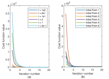
Fig. 2 illustrates the convergence behavior of Algorithm 2 under various barrier parameters and initial points. Fig. 2 (a) demonstrates the impact of the barrier parameter $t$ on the convergence. It is observed that a smaller $t$ leads to faster convergence but may result in a higher final cost, while a larger $t$ slows down the convergence but yields a lower final cost. This trade-off between convergence speed and solution quality is consistent with the theory of interior-point methods. The results suggest that a well-tuned barrier parameter, e.g., $t=1$, can strike a balance between convergence speed and optimality. Additionally, the algorithm exhibits stable convergence for a wide range of $t$ values from 0.5 to 100, indicating its robustness to the choice of barrier parameter. Fig. 2 (b) reveals that the proposed algorithm converges within limited iterations for all considered initial points, showcasing its robustness to initialization. However, the choice of initial point does affect the convergence speed and the final objective value. To improve the solution quality, we run the algorithm with different random initial points and select the best local optimum.

Refer to caption
Figure 3: Communication spectral efficiency versus received SNR for different subarray layouts.

Then, we investigate the impact of different subarray distributions on the performance of ISAC systems. With a fixed number of subarrays $K$ and antennas per subarray $M$, we consider three modular array configurations: random subarray layout (denoted as ”random”), where the subarrays are randomly distributed; uniform subarray layout (denoted as ”uniform”), where the subarrays are uniformly distributed; and collocated subarray layout (denoted as ”collocated”), where the subarrays are closely spaced with a half-wavelength inter-subarray spacing. For notational convenience, we denote Algorithm 1 as RM-JGD and Algorithm 2 as SDR-RRS.

Fig. 3 illustrates the user’s communication spectral efficiency versus the received SNR for both SDR-RRS and RM-JGD under three modular array configurations. It is noted that for both algorithms, the modular arrays with random and uniform subarray layouts achieve similar communication spectral efficiencies, surpassing the collocated subarray layout. Moreover, the performance gap widens as the SNR increases, indicating that for modular arrays with the same $K$ and $M$, widely spaced subarray distributions outperform the traditional collocated distribution. This superiority stems from the more pronounced near-field spherical wave characteristics of widely spaced subarrays, which enhance the channel rank and spatial multiplexing gain. Furthermore, SDR-RRS consistently outperforms RM-JGD across all array configurations, showcasing its ability to better handle the non-convex optimization problem and find higher-quality locally optimal solutions.

Refer to caption
Figure 4: Communication spectral efficiency versus sensing SCNR threshold for different numbers of RF chains.

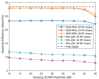
We then present the communication spectral efficiency with different sensing SCNR thresholds in Fig. 4 to show the trade-off between sensing and communication performance. The performance of fully digital beamforming serves as an upper bound for comparison. As the sensing SCNR threshold increases, the communication spectral efficiency decreases for both algorithms, with a more severe performance degradation observed for the case with fewer RF chains. Specifically, for low sensing SCNR thresholds, the communication spectral efficiency of SDR-RRS with a hybrid beamformer using 24 RF chains closely approaches the fully digital performance. However, the performance gap widens at higher SCNR thresholds. Besides, the SDR-RRS algorithm consistently outperforms the RM-JGD algorithm in terms of communication spectral efficiency across all SCNR thresholds and RF chain configurations, indicating its superior ability to strike a balance between communication and sensing performances.

Refer to caption
Figure 5: Communication spectral efficiency versus user distance for different subarray scales based on SDR-RRS algorithm.

Fig. 5 illustrates the impact of subarray scale on the communication performance of SDR-RRS algorithm in modular XL-MIMO ISAC systems. The total array aperture $S$ and the number of antennas $N_{t}=192$ are kept constant, while the number of antennas per subarray $M$ is varied as 16, 24, 32, 48, and 64, resulting in the corresponding number of subarrays $K$ being 12, 8, 6, 4, and 3, respectively. It can be observed that the optimal subarray scale for maximizing the communication spectral efficiency varies with the user distance. For user distances less than $25\mathrm{m}$, the subarray scale of $M=48$ outperforms the others, while for distances beyond $25\mathrm{m}$, the subarray scale of $M=64$ achieves the highest communication spectral efficiency. A larger number of subarrays $K$ provides higher spatial multiplexing gains, but a smaller $M$ reduces the beamforming gain. Thus, the optimal subarray scale at different distances represents a trade-off between spatial multiplexing and beamforming gains for maximizing the communication performance. Moreover, the performance gap between subarray scales diminishes with increasing distance due to the transition from near-field spherical wavefronts, which enhance spatial multiplexing for larger $K$ at shorter ranges, to far-field planar wavefronts where such gains diminish.

Refer to caption
Figure 6: Communication spectral efficiency versus user distance for different numbers of NLoS paths.

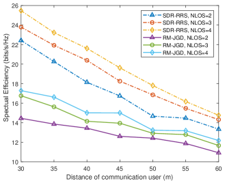
Fig. 6 illustrates the impact of user distance and the number of NLoS paths on the communication spectral efficiency for both the SDR-RRS and RM-JGD algorithms. The communication spectral efficiency of both Algorithms decreases with increasing user distance due to increased path loss and diminishing near-field spherical wave characteristics, which reduce the channel rank and limit the number of independent spatial streams available for communication. It is noted that SDR-RRS consistently outperforms RM-JGD for all considered scenarios, showcasing its superior performance. Moreover, the performance gap between the two algorithms widens as the number of NLoS paths increases, highlighting the ability of SDR-RRS to better exploit multipath propagation for higher communication spectral efficiencies. It also reveals that even for distant users, a rich scattering environment with abundant NLoS paths can sustain high communication spectral efficiencies, highlighting the potential of exploiting multipath propagation to enhance cell-edge performance.

Refer to caption
Figure 7: Communication spectral efficiency versus sensing SCNR threshold for different levels of overlap between communication channel scatterers and sensing interference.

We then investigate the impact of the overlap between communication channel scatterers and sensing interference on the communication-sensing performance tradeoff. The overlap parameter represents the number of scatterers that coincide with the sensing interference, with overlap values 0 indicating no overlap and thus low correlation between the communication and sensing channels. Overlap values of 1 and 2 represent that one and two scatterers in the environment also act as interference sources for the sensing targets, respectively. As shown in Fig. 7, for both the SDR-RRS and RM-JGD algorithms, a higher overlap value yields a higher communication spectral efficiency at the same sensing SCNR threshold, indicating that the system achieves a better communication-sensing tradeoff. This is because that the correlation between the communication and sensing channels increase as the number of overlapping scatterers and interference sources grows, leading to more efficient resource utilization for the proposed ISAC system.

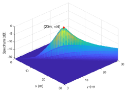
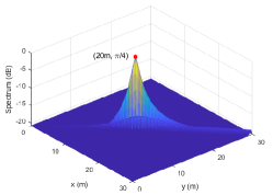
In Fig. 8, the normalized mutiple signal classification (MUSIC) spectrum obtained by the proposed SDR-RRS algorithm is compared for $M=32$ with varying numbers of subarrays $K$, over a grid spanning $x\in[0:0.06:30]$ m and $y\in[0:0.06:30]$ m. The peak of the spectrum is consistently observed at the actual target location $(20\mathrm{m},\pi/4)$ for all values of $K$. Notably, the main lobe width containing the peak value narrows as $K$ increases, indicating enhanced range resolution at the same angular direction. This behavior can be attributed to the spherical wavefront characteristic across subarrays, which becomes more pronounced with increasing $K$, leading to improved range estimation accuracy. The results demonstrate that augmenting the number of subarrays can significantly enhance the range resolution capability of the MUSIC algorithm, thereby enabling more precise target localization.

Refer to caption
(a) M=32, K=8
Refer to caption
(b) M=32, K=12
Refer to caption
(c) M=32, K=16
Figure 8: Normalized MUSIC spectrum for different numbers of subarrays $K$ with $M=32$ antennas per subarray.

VI Conclusion

In this paper, we have proposed a novel modular XL-MIMO ISAC framework and developed the low-complexity hybrid beamforming algorithms. By exploiting the structural similarity between the communication and sensing channels based on the HSPM, we have derived a closed-form solution for the optimal analog beamforming matrix and transformed the joint analog-digital design problem into a lower-dimensional digital beamformer optimization. To address the rank-constrained digital beamformer optimization, we have proposed a manifold-based algorithm for reduced complexity and a SDR-based method for near-optimal solutions.

Extensive simulations have validated the effectiveness of the proposed framework and algorithms. The simulations reveal that increasing the number of subarrays enhances the spatial multiplexing gain and improves the range resolution for sensing. The presence of NLoS paths and the correlation between communication and sensing channels are shown to have a significant impact on performances of the ISAC system. Moreover, the optimal subarray scale is found to vary with the user distance, highlighting the trade-off between beamforming gain and spatial multiplexing gain. These findings offer useful guidelines for the deployment of modular XL-MIMO ISAC systems in various practical scenarios.

Appendix A Proof of Theorem 1

Based on the method proposed in [31, App. C], let

$$\mathbf{R}_{X}^{*}=\bm{\Delta}\bm{\Delta}^{\mathrm{H}}.$$ (60)

We can decompose $\bm{\Delta}$ as

$$\bm{\Delta}=P_{\tilde{U}}\bm{\Delta}+\mathbf{P}_{\tilde{U}}^{\perp}\bm{\Delta},$$ (61)

where $\mathbf{P}_{\tilde{U}}=\mathbf{{\tilde{U}}}(\mathbf{{\tilde{U}}}^{H}\mathbf{{\tilde{U}}})^{-1}\mathbf{{\tilde{U}}}^{H}$ denotes the orthogonal projection onto the subspace spanned by the columns of $\mathbf{{\tilde{U}}}$ in (35a), and $\mathbf{P}_{\tilde{U}}^{\perp}=\mathbf{I}-\mathbf{P}_{\tilde{U}}$. Furthermore, we can decompose $\bm{\Delta}$ additively as

$$\mathbf{R}_{X}^{*}=\mathbf{P}_{\tilde{U}}\bm{\Delta}\bm{\Delta}^{H}\mathbf{P}_{\tilde{U}}+\tilde{\mathbf{R}}_{X},$$ (62)

with

$${{\widetilde{\mathbf{R}}}_{X}}=\mathbf{P}_{{\tilde{U}}}^{\bot}\mathbf{\Delta}{{\mathbf{\Delta}}^{H}}\mathbf{P}_{{\tilde{U}}}^{\bot}+{{\mathbf{P}}_{{\tilde{U}}}}\mathbf{\Delta}{{\mathbf{\Delta}}^{H}}\mathbf{P}_{{\tilde{U}}}^{\bot}+\mathbf{P}_{{\tilde{U}}}^{\bot}\mathbf{\Delta}{{\mathbf{\Delta}}^{H}}{{\mathbf{P}}_{{\tilde{U}}}}.$$ (63)

By utilizing the property of orthogonal projection matrices that ${{\mathbf{P}}_{{\tilde{U}}}}\mathbf{\tilde{U}}=\mathbf{\tilde{U}}$ and ${{\mathbf{\tilde{U}}}^{H}}{{\mathbf{P}}_{{\tilde{U}}}}={{\mathbf{\tilde{U}}}^{H}}$, we can obtain that

$${{\mathbf{\tilde{U}}}^{H}}{{\widetilde{\mathbf{R}}}_{X}}\mathbf{\tilde{U}}=\bm{0}.$$ (64)

According to (34), utilizing the property of permutation matrix that $\mathbf{P}^{-1}=\mathbf{P}^{T}$, we have

$$\mathbf{U}=\mathbf{\tilde{U}}\mathbf{P}^{T}.$$ (65)

Therefore, by substituting (65) into (29) and (30), $\mathbf{V}_{c}$ and ${{\mathbf{g}}_{t}}\left({{\mathbf{l}}_{q}}\right),\forall q$ can be expressed as linear transformations of $\mathbf{\tilde{U}}$, namely

$${{\mathbf{g}}_{t}}\left({{\mathbf{l}}_{q}}\right)=\mathbf{\tilde{U}}\mathbf{P}^{T}\mathbf{\tilde{{\bm{\nu}}}}_{tq},\ \forall q,$$ (66)
$${{\mathbf{V}}_{c}}=\mathbf{\tilde{U}}\mathbf{P}^{T}\mathbf{\tilde{T}}.$$ (67)

Thus, it can be readily verified that

$\displaystyle{{\mathbf{g}}_{t}}{{\left({{\mathbf{l}}_{q}}\right)}^{H}}{{\mathbf{\tilde{R}}}_{X}}{{\mathbf{g}}_{t}}\left({{\mathbf{l}}_{q}}\right)$ $\displaystyle=\widetilde{\bm{\nu}}_{tq}^{H}\mathbf{P}{{\mathbf{\tilde{U}}}^{H}}{{\mathbf{\tilde{R}}}_{X}}\mathbf{\tilde{U}}{{\mathbf{P}}^{T}}{{\widetilde{\bm{\nu}}}_{tq}}=0,\forall q,$ (68a)
$\displaystyle\mathbf{V}_{c}^{H}{{\mathbf{\tilde{R}}}_{X}}{{\mathbf{V}}_{c}}$ $\displaystyle={{\mathbf{\tilde{T}}}^{H}}\mathbf{P}{{\mathbf{\tilde{U}}}^{H}}{{\mathbf{\tilde{R}}}_{X}}\mathbf{\tilde{U}}{{\mathbf{P}}^{T}}\mathbf{\tilde{T}}={{\mathbf{0}}}.$ (68b)

Based on the SVD of ${{\mathbf{H}}_{c}}$, the achievable communication spectral efficiency in (14) can be rewritten accordingly as

$$C=\log\det\left(\mathbf{I}+\frac{1}{\sigma_{c}^{2}}{\mathbf{\Sigma}_{c}}\mathbf{V}_{c}^{H}{{\mathbf{R}}_{X}}{{\mathbf{V}}_{c}}\right).$$ (69)

By substituting (62) into (20) and (69) and observing (68), we can conclude that the sensing SCNR and the achievable communication spectral efficiency are both independent of ${{\mathbf{\tilde{R}}}_{X}}$. Besides, we note that

$$\text{tr}\left({{{\mathbf{\tilde{R}}}}_{X}}\right)=\text{tr}\left(\mathbf{P}_{{\tilde{U}}}^{\bot}\mathbf{\Delta}{{\mathbf{\Delta}}^{H}}\mathbf{P}_{{\tilde{U}}}^{\bot}\right)=\left\|\mathbf{\Delta}^{H}\mathbf{P}_{{\tilde{U}}}^{\bot}\right\|_{F}^{2}\geq 0,$$ (70)

which means that the ${{\mathbf{\tilde{R}}}_{X}}$ component does not contribute to either the communication or sensing performance, but only consumes the transmit power. Thus, we must have $\text{tr}({{{\mathbf{\tilde{R}}}}_{X}})=0$ to satisfy the transmit power constraint. The equality in (70) holds if and only if $\mathbf{\Delta}^{H}\mathbf{P}_{{\tilde{U}}}^{\bot}=\mathbf{0}$, and it can be observed from (63) that this implies ${{\mathbf{\tilde{R}}}_{X}}=\mathbf{0}$.

Therefore, the optimal covariance matrix $\mathbf{R}_{X}^{*}$ can be written as

$$\mathbf{R}_{X}^{*}={{\mathbf{P}}_{{\tilde{U}}}}\mathbf{\Delta}{{\mathbf{\Delta}}^{H}}{{\mathbf{P}}_{{\tilde{U}}}}\triangleq\mathbf{\tilde{U}\Lambda}{{\mathbf{\tilde{U}}}^{H}},$$ (71)

where $\mathbf{\Lambda}$ is a positive semi-definite matrix, and it can be given by

$$\mathbf{\Lambda}={{({{\mathbf{\tilde{U}}}^{H}}\mathbf{\tilde{U}})}^{-1}}{{\mathbf{\tilde{U}}}^{H}}\mathbf{\Delta}{{\mathbf{\Delta}}^{H}}\mathbf{\tilde{U}}{{({{\mathbf{\tilde{U}}}^{H}}\mathbf{\tilde{U}})}^{-1}},$$ (72)

which completes the proof.

References

  • [1] X. Mu, J. Xu, Y. Liu, and L. Hanzo, “Reconfigurable intelligent surface-aided near-field communications for 6G: Opportunities and challenges,” IEEE Veh. Technol. Mag., vol. 19, no. 1, pp. 65–74, Jan. 2024.
  • [2] X. Mu, Z. Wang, and Y. Liu, “NOMA for integrating sensing and communications towards 6G: A multiple access perspective,” IEEE Wirel. Commun., pp. 1–8, 2023.
  • [3] Y. Liu, Z. Wang, J. Xu, C. Ouyang, X. Mu, and R. Schober, “Near-field communications: A tutorial review,” IEEE Open J. Commun. Soc., vol. 4, pp. 1999–2049, Aug. 2023.
  • [4] J. Cong, C. You, J. Li, L. Chen, B. Zheng, Y. Liu, W. Wu, Y. Gong, S. Jin, and R. Zhang, “Near-field integrated sensing and communication: Opportunities and challenges,” arXiv preprint arXiv:2310.01342, 2023.
  • [5] Z. Wang, X. Mu, and Y. Liu, “Near-field integrated sensing and communications,” IEEE Commun. Lett., vol. 27, no. 8, pp. 2048–2052, Aug. 2023.
  • [6] D. Galappaththige, S. Zargari, C. Tellambura, and G. Y. Li, “Near-field ISAC: Beamforming for multi-target detection,” IEEE Wireless Commun. Lett., pp. 1–1, May. 2024.
  • [7] B. Zhao, C. Ouyang, Y. Liu, X. Zhang, and H. V. Poor, “Modeling and analysis of near-field ISAC,” IEEE J. Sel. Topics Signal Process., pp. 1–16, Apr. 2024.
  • [8] L. Yan, Y. Chen, C. Han, and J. Yuan, “Joint inter-path and intra-path multiplexing for terahertz widely-spaced multi-subarray hybrid beamforming systems,” IEEE Trans. Commun., vol. 70, no. 2, pp. 1391–1406, Dec. 2022.
  • [9] X. Li, H. Lu, Y. Zeng, S. Jin, and R. Zhang, “Near-field modeling and performance analysis of modular extremely large-scale array communications,” IEEE Commun. Lett., vol. 26, no. 7, pp. 1529–1533, 2022.
  • [10] X. Li, Z. Dong, Y. Zeng, S. Jin, and R. Zhang, “Multi-user modular XL-MIMO communications: Near-field and beam focusing pattern and user grouping,” arXiv preprint arXiv:2308.11289, Aug. 2023.
  • [11] H. Lu, Y. Zeng, C. You, Y. Han, J. Zhang, Z. Wang, Z. Dong, S. Jin, C.-X. Wang, T. Jiang et al., “A tutorial on near-field XL-MIMO communications towards 6G,” arXiv preprint arXiv:2310.11044, Oct. 2023.
  • [12] S. Yang, X. Chen, Y. Xiu, W. Lyu, Z. Zhang, and C. Yuen, “Performance bounds for near-field localization with widely-spaced multi-subarray mmwave/THz MIMO,” IEEE Trans. Wirel. Commun., pp. 1–1, Mar. 2024.
  • [13] Y. Chen and L. Dai, “Non-stationary channel estimation for extremely large-scale MIMO,” IEEE Trans. Wirel. Commun., pp. 1–1, Dec. 2023.
  • [14] H. Shen, L. Yan, C. Han, and H. Liu, “Alternating optimization based hybrid beamforming in terahertz widely-spaced multi-subarray systems,” in Proc. IEEE Global Commun. Conf. (Globecom), Dec. 2022, pp. 1760–1765.
  • [15] X. Wang, Z. Fei, J. A. Zhang, and J. Xu, “Partially-connected hybrid beamforming design for integrated sensing and communication systems,” IEEE Trans. Commun., vol. 70, no. 10, pp. 6648–6660, Aug. 2022.
  • [16] Y. Chen, R. Li, C. Han, S. Sun, and M. Tao, “Hybrid spherical- and planar-wave channel modeling and estimation for terahertz integrated UM-MIMO and IRS systems,” IEEE Trans. Wirel. Commun., pp. 1–1, May 2023.
  • [17] Y. Chen, L. Yan, and C. Han, “Hybrid spherical- and planar-wave modeling and dcnn-powered estimation of terahertz ultra-massive MIMO channels,” IEEE Trans. Commun., vol. 69, no. 10, pp. 7063–7076, July 2021.
  • [18] X. Zhu, Y. Liu, and C.-X. Wang, “Sub-array-based millimeter wave massive MIMO channel estimation,” IEEE Wireless Commun. Lett., vol. 12, no. 9, pp. 1608–1612, June 2023.
  • [19] Y. Xing, T. S. Rappaport, and A. Ghosh, “Millimeter wave and sub-THz indoor radio propagation channel measurements, models, and comparisons in an office environment,” IEEE Commun. Lett., vol. 25, no. 10, pp. 3151–3155, June 2021.
  • [20] G. Gougeon, Y. Corre, and M. Z. Aslam, “Ray-based deterministic channel modelling for sub-THz band,” in Proc. IEEE Int. Symp. Pers. Indoor Mobile Radio Commun. (PIMRC Workshops), Sept. 2019, pp. 1–6.
  • [21] X. Gao, L. Dai, S. Han, C.-L. I, and R. W. Heath, “Energy-efficient hybrid analog and digital precoding for mmwave MIMO systems with large antenna arrays,” IEEE J. Sel. Areas Commun., vol. 34, no. 4, pp. 998–1009, Mar. 2016.
  • [22] L. Chen, Z. Wang, Y. Du, Y. Chen, and F. R. Yu, “Generalized transceiver beamforming for dfrc with MIMO radar and MU-MIMO communication,” IEEE J. Sel. Areas Commun., vol. 40, no. 6, pp. 1795–1808, 2022.
  • [23] Z. Cheng, L. Wu, B. Wang, M. R. B. Shankar, and B. Ottersten, “Double-phase-shifter based hybrid beamforming for mmwave DFRC in the presence of extended target and clutters,” IEEE Trans. Wirel. Commun., vol. 22, no. 6, pp. 3671–3686, Nov. 2023.
  • [24] J. Capon, “High-resolution frequency-wavenumber spectrum analysis,” Proc. IEEE, vol. 57, no. 8, pp. 1408–1418, Aug. 1969.
  • [25] H. Yu and V. K. N. Lau, “Rank-constrained schur-convex optimization with multiple trace/log-det constraints,” IEEE Trans. Signal Process., vol. 59, no. 1, pp. 304–314, Oct. 2011.
  • [26] J. Manton, “Optimization algorithms exploiting unitary constraints,” IEEE Trans. Signal Process., vol. 50, no. 3, pp. 635–650, Mar. 2002.
  • [27] G. H. Golub and C. F. Van Loan, Matrix computations.   JHU press, 2013.
  • [28] A. Edelman, T. A. Arias, and S. T. Smith, “The geometry of algorithms with orthogonality constraints,” SIAM journal on Matrix Analysis and Applications, vol. 20, no. 2, pp. 303–353, 1998.
  • [29] K. Fujisawa, M. Kojima, and K. Nakata, “Exploiting sparsity in primal-dual interior-point methods for semidefinite programming,” Mathematical Programming, vol. 79, pp. 235–253, 1997.
  • [30] 3GPP, “Study on channel model for frequencies from 0.5 to 100 GHz,” 3rd Generation Partnership Project (3GPP), Sophia Antipolis, France, 3GPP Rep. (TR) 38.901, 2024, version 18.0.0. [Online]. Available: http://www.3gpp.org/DynaReport/38901.html
  • [31] J. Li, L. Xu, P. Stoica, K. W. Forsythe, and D. W. Bliss, “Range compression and waveform optimization for MIMO radar: A cramer–rao bound based study,” IEEE Trans. Signal Process., vol. 56, no. 1, pp. 218–232, Dec. 2008.