On semi-implicit schemes for the incompressible Euler equations via the vanishing viscosity limit

Abstract.

A new type of systematic approach to study the incompressible Euler equations numerically via the vanishing viscosity limit is proposed in this work. We show the new strategy is unconditionally stable that the $L^{2}$-energy dissipates and $H^{s}$-norm is uniformly bounded in time without any restriction on the time step. Moreover, first-order convergence of the proposed method is established including both low regularity and high regularity error estimates. The proposed method is extended to full discretization with a newly developed iterative Fourier spectral scheme. Another main contributions of this work is to propose a new integration by parts technique to lower the regularity requirement from $H^{4}$ to $H^{3}$ in order to perform the $L^{2}$-error estimate. To our best knowledge, this is one of the very first work to study incompressible Euler equations by designing stable numerical schemes via the inviscid limit with rigorous analysis. Furthermore, we will present both low and high regularity errors from numerical experiments and demonstrate the dynamics in several benchmark examples.

1. Introduction

1.1. Introduction to the models and the historical review

In this presenting paper we are interested in the incompressible Euler equations in a periodic domain $\mathbb{T}^{d}=(\mathbb{R}/(2\pi))^{d}$ with dimension $d=2,3$:

$$\begin{cases}&\partial_{t}u+u\cdot\nabla u+\nabla p=0,\qquad\nabla\cdot u=0;\\ &u|_{t=0}=u_{0}.\end{cases}$$ (1.1)

Here the solution $u:\mathbb{R}^{+}\times\mathbb{T}^{d}\to\mathbb{R}^{d}$ is the velocity field and $p:\mathbb{R}^{+}\times\mathbb{T}^{d}\to\mathbb{R}$ is the pressure. In particular, the velocity field $u$ satisfies the divergence-free condition $\nabla\cdot u=0$ to guarantee the system is incompressible. In this work we are also concerned of the corresponding incompressible Navier-Stokes system (NS):

$$\begin{cases}&\partial_{t}u^{\nu}+u^{\nu}\cdot\nabla u^{\nu}+\nabla p^{\nu}=\nu\Delta u^{\nu},\qquad\nabla\cdot u^{\nu}=0;\\ &u^{\nu}|_{t=0}=u_{0}.\end{cases}$$ (1.2)

It is worth mentioning here that the solution pair depends on the viscosity parameter $\nu$ and therefore we emphasize it as $(u^{\nu},p^{\nu})$.

Both the Euler equations and Navier-Stokes equations play fundamental roles in the fluid dynamics. The Euler equations provide simplified models of fluid flows, which are useful in scenarios where the fluid behaves more like an ideal fluid, such as in many aerodynamic applications. Unlike the Euler equations, the Navier-Stokes equations are applicable to both inviscid and viscous fluid flows due to the viscosity. Therefore Navier-Stokes equations are widely used in blood flows, air flow around an airfoil, and ocean currents models. The local well-posedness of the Euler and Navier-Stokes equations were discussed in [18, 31, 32] and the references therein. More specifically, for the two-dimensional Euler equations, Yudovich [37] established the existence and uniqueness of global weak solutions. Beale, Kato and Majda [4] provided the BKM criterion for determining the global existence of strong solutions to the Euler equations. Kiselev and Sverak [25] obtained a lower bound estimate for the double exponential growth of solutions to two-dimensional Euler equations on bounded domains. For the Navier-Stokes equations, Leray [26] established the existence of global weak solutions. Fujita and Kato [16] first proved global solutions of the Navier-Stokes equations with small initial value $u_{0}\in\dot{H}^{\frac{1}{2}}$. Well-posedness of mild solutions to the 3D NS-system has been studied by Lei and Lin in [27].

On the contrary, for the ill-posedness direction of the fluid systems, Bourgain and Li [5] obtained strong ill-posedness of the Euler equations in borderline sobolev spaces. Recently, Elgindi [15] proved that low regular solutions of the Euler equations blow up in finite time. Bourgain and Pavlovic [6] obtained the ill-posedness of solutions to the Navier-Stokes equations. Moreover, it is also worth mentioning that the non-uniqueness of low regular solutions to fluid equations have been studied in [1, 7, 8, 12, 24, 30] etc.

The exact solutions cannot be derived in most scenarios, therefore a great many numerical methods to study the Euler and Navier-Stokes equations have been proposed including the backward Euler differentiation method [35], finite element methods [21, 22, 28], finite difference methods [9, 13, 14], spectral methods [17], the Lagrange–Galerkin method [20, 34], and the projection method for time discretization [10, 23, 13, 14]. The convergence of numerical solutions to the fluid equations above was all proved assuming a sufficiently smooth solution. It is also worth mentioning that recently Li, Ma and Schratz [29] developed low regularity methods dating back to Rousset-Schratz [33], Bai-Li-Wu [3] and Wu-Zhao [36], where an exponential integrator can help to reduce the regularity requirements; however in this work we will not dig further in this direction.

The Euler and NS models are closely related; indeed the Euler equations can be viewed as a vanishing viscosity limit of Navier-Stokes equations, cf. [11, 31, 18]. In more details, Masmoudi in [31] proved the $H^{s-2}$ convergence of the NS solution $u^{\nu}$ to the Euler solution $u$ as $\nu\to 0$ assuming the initial data $u_{0}\in H^{s}$ for $s>2$. The rate of convergence was proved to be $\|u^{\nu}-u\|_{H^{s-2}}=O(\nu)$. Moreover, the $H^{s}$ convergence is also proved with help of a smoothing mollification of the initial data. In effect such mollification can be understood as a Fourier truncation; thus we are motivated to solve it by implementing Fourier spectral methods. Consequently, one of the modest goals of this presenting paper is to provide a systematic approach to study the Euler equations numerically by the Fourier spectral method via the vanishing viscosity limit. Another main contributions of this work is to propose a new integration by parts technique to lower the regularity requirement from $H^{4}$ to $H^{3}$ in order to perform the $L^{2}$-error estimate. To our best knowledge, this is one of the very first work to study incompressible Euler equations by designing stable numerical schemes via the inviscid limit with rigorous analysis.

The first semi-implicit Fourier spectral scheme we consider is the following:

$$\begin{cases}&\frac{u^{n+1}-u^{n}}{\tau}+\Pi_{N}(u^{n}\cdot\nabla u^{n+1})+\nabla p^{n}=\nu\Delta u^{n+1},\\ &\mathop{\rm div}u^{n+1}=0,\\ &u^{0}=\Pi_{N}u_{0},\end{cases}$$ (1.3)

where $\tau$ is the time step. For $N\geq 2$, we introduce the space

$$X_{N}=\text{span}\left\{\cos(k\cdot x)\ ,\ \sin(k\cdot x):\ \ k=(k_{1},k_{2})\in\mathbb{Z}^{2}\ ,\ |k|_{\infty}=\max\{|k_{1}|,|k_{2}|\}\leq N\right\}\ .$$

Then we define $\Pi_{N}$ to be the truncation operator of Fourier modes $|k|_{\infty}\leq N$. $\Pi_{N}u_{0}\in X_{N}$ and by induction, we have $u^{n}\in X_{N}\ ,\forall n\geq 0$. Moreover in (1.3) the viscosity term $\nu\Delta u^{n+1}$ is unknown and the nonlinear term $u^{n}\cdot\nabla u^{n+1}$ is linear with respect to $u^{n+1}$. In addition we can further derive that $\mathop{\rm div}u^{n}=0$ for all $n$ by induction. To solve $u^{n+1}$, we recall the Leray projection $\mathbb{P}$, namely the $L^{2}$-orthogonal projection onto the divergence-free subspace: for any $v\in L^{2}$ we have $\mathbb{P}v=v-\nabla q$, where $q\in H^{1}$ solves the following Poisson equation under periodic boundary conditions:

$$\Delta q=\nabla\cdot v.$$

Then we apply the Leray projection $\mathbb{P}$ to derive that

$$\frac{u^{n+1}-u^{n}}{\tau}+\mathbb{P}\Pi_{N}(u^{n}\cdot\nabla u^{n+1})=\nu\Delta u^{n+1}.$$ (1.4)

In fact we will solve the Euler equations from the first order semi-implicit scheme (1.4). We shall show our scheme (1.4) preserves energy stability (dissipates in $n$) and preserves regularity boundedness; moreover the $L^{2}$ error will be shown with numerical evidence. Our main results are stated below.

1.2. Main results

To start with, we first present an unconditional stability result of the semi-implicit scheme (1.3) or (1.4).

Theorem 1.1 (Unconditional stability).

Consider the Euler equations (1.1) in $\mathbb{T}^{2}$ with periodic boundary conditions and we solve (1.1) using the semi-implicit Fourier spectral scheme (1.3). Assume that the initial data $u_{0}\in H^{s}(\mathbb{T}^{2})$ for any $s>2$ then there exist $T>0$ such that the following statements hold for any $M\in\mathbb{Z}^{+}$ and $n\leq M$ without any restriction on the time step $\tau=\frac{T}{M}$.

(i):

The $L^{2}$ energy dissipates in time:

$$\|u^{n+1}\|_{L^{2}}\leq\|u^{n}\|_{L^{2}}.$$ (1.5)

(ii):

The $H^{s}$ norm is uniformly bounded:

$$\sup_{n}\|u^{n}\|_{H^{s}}\leq 4\|u_{0}\|_{H^{s}}.$$ (1.6)

Remark 1.1.

From the local well-posedness theory of nonlinear PDE, one usually needs to take sufficiently small $T$ to handle $\mathbb{P}\Pi_{N}(u^{n}\cdot\nabla u^{n+1})$, otherwise the solution may behave as a double exponential growth (cf. [25]). Through the commutator estimates and embedding theory $\|\nabla f\|_{L^{\infty}}\leq C_{s}\|f\|_{H^{s}}$, where $C_{s}>0$ only depends on $s>2$, we found that $C_{s}T\|u^{n}\|_{H^{s}}\leq 1$ is the key to completing uniformly bounded estimates. This together with (1.6) allows us to take the time period $T=\frac{1}{4C_{s}\|u_{0}\|_{H^{s}}}$. However in practice we do not need to consider such short time period, we refer the readers to Section 6 for more details.

It is worth mentioning that if we further require that the size of the time step $\tau$ is small then an extra $H^{1}$-energy dissipation can be derived:

Corollary 1.2 ($H^{1}$-energy stability).

Let the same assumptions in Theorem 1.1 hold. We further assume $\tau\leq c\nu$ for some absolute constant $c>0$ that can be computed, then the following $\dot{H}^{1}$ energy dissipation is true:

$$\|\nabla u^{n+1}\|_{2}+\|\nabla(u^{n+1}-u^{n})\|_{2}\leq\|\nabla u^{n}\|_{2}.$$

As a result, the $H^{1}$ energy stability follows: $\|u^{n+1}\|_{H^{1}}\leq\|u^{n}\|_{H^{1}}$.

The error can be controlled by the following theorem.

Theorem 1.3 (Error estimates).

Let the same assumptions in Theorem 1.1 hold. Assume that $v(t,x)$ is the exact solution to (1.1) with the same initial condition $u_{0}\in H^{s}(\mathbb{T}^{2})$ for $s\geq 3$. Then the following error estimates hold.

(i):

The $L^{2}$-error estimate holds:

$$\sup_{n}\|u^{n+1}-v\left(t_{n+1}\right)\|_{L^{2}}\leq C_{1}(\nu+\tau+N^{-s+1});$$ (1.7)

(ii):

Additionally if $u_{0}\in H^{s+3}(\mathbb{T}^{2})$, then the $H^{s}$-error estimate holds:

$$\sup_{n}\|u^{n+1}-v\left(t_{n+1}\right)\|_{H^{s}}\leq C_{2}(\tau+N^{-2}+N^{2}\nu).$$ (1.8)

Here the constant $C_{1}>0$ above only depends on the initial condition $\|u_{0}\|_{H^{s}}$ and $C_{2}>0$ depends only on $\|u_{0}\|_{H^{s+3}}$.

Remark 1.2.

It is worth mentioning that (see [29] for example) in order to obtain an $L^{2}$-error estimate, the usual semi-implicit method may require that the solution to be $H^{4}$. However, our method proposes a systematic way to lower that requirement to $H^{3}$ through an integration by parts technique.

Remark 1.3.

We discuss more about the $H^{s}$ error estimate in Theorem 1.3 here. Note that the term $N^{2}\nu$ may lead to a large error as $N\to\infty$ (we refer the readers to Table 3 in Section 6) therefore we need $\nu\ll N^{-2}$ in the inviscid limit sense in order to approximate the solutions to the Euler equations. However, such term will not appear when solving the NS system with fixed $\nu$. Therefore our semi-implicit scheme is stable and accurate in solving NS system too.

Remark 1.4.

It is also worth mentioning the semi-implicit scheme adopted by Guo and Zou in [17]:

$$\frac{u^{n+1}-u^{n}}{\tau}+\mathbb{P}\Pi_{N}(u^{n}\cdot\nabla u^{n})=\nu\Delta u^{n+1}.$$ (1.9)

Their scheme (1.9) is easier to compute since the nonlinear term is treated known from the previous time step $n$, but it seems very challenging to prove the stability result as in Theorem 1.1 due to the nonlinearity. Moreover, the error estimate for the scheme (1.9) requires that $\tau\leq c_{1}N^{-1}$ for some small $c_{1}$ in [17]. On the other hand, the new scheme (1.4) is harder to compute numerically via the Fourier spectral method; indeed as suggested in [29], a convolution type method is required. In this paper we present a new iteration idea that avoid the long computation and more details can be found in Section 5. One can immediately derive as a direct corollary of Theorem 1.3 that the schemes (1.3) and (1.9) differ by an $O(\tau)$ error.

1.3. Organization of the presenting paper

The presenting paper is organized as follows. In Section 2 we list the notation and preliminaries including several useful lemmas. In Section 3 we prove Theorem 1.1 and the proof to Theorem 1.3 can be found in Section 4. We give details of the full discretization of the scheme through a new iterative Fourier spectral method in Section 5. We will provide numerical evidence in Section 6 and the proof of Corollary 1.2 and Lemma 2.2 can be found in the Appendix A and Appendix B respectively.

2. Notation and preliminaries

2.1. Notation

Throughout this paper, for any two (non-negative in particular) quantities $X$ and $Y$, we denote $X\lesssim Y$ if $X\leq CY$ for some constant $C>0$. Similarly $X\gtrsim Y$ if $X\geq CY$ for some $C>0$. We denote $X\sim Y$ if $X\lesssim Y$ and $Y\lesssim X$. The dependence of the constant $C$ on other parameters or constants are usually clear from the context and we will often suppress this dependence. We shall denote $X\lesssim_{Z_{1},Z_{2},\cdots,Z_{k}}Y$ if $X\leq CY$ and the constant $C$ depends on the quantities $Z_{1},\cdots,Z_{k}$.

For any two quantities $X$ and $Y$, we shall denote $X\ll Y$ if $X\leq cY$ for some sufficiently small constant $c$. The smallness of the constant $c$ is usually clear from the context. The notation $X\gg Y$ is similarly defined. Note that our use of $\ll$ and $\gg$ here is different from the usual Vinogradov notation in number theory or asymptotic analysis.

We define $[A,B]$ to be $AB-BA$, namely the usual commutator.

For a real-valued function $u:\Omega\to\mathbb{R}$ we denote its usual Lebesgue $L^{p}$-norm by

$$\|u\|_{p}=\|u\|_{L^{p}(\Omega)}=\begin{cases}&\left(\int_{\Omega}|u|^{p}\ dx\right)^{\frac{1}{p}},\quad 1\leq p<\infty;\\ &\operatorname{esssup}_{x\in\Omega}|u(x)|,\quad p=\infty.\end{cases}$$

Similarly, we use the weak derivative in the following sense: For $u$, $v\in L^{1}_{loc}(\Omega)$, (i.e they are locally integrable); $\forall\phi\in C^{\infty}_{0}(\Omega)$, i.e $\phi$ is infinitely differentiable (smooth) and compactly supported; and

$$\int_{\Omega}u(x)\ \partial^{\alpha}\phi(x)\ dx=(-1)^{\alpha_{1}+\cdots+\alpha_{n}}\int_{\Omega}v(x)\ \phi(x)\ dx,$$

then $v$ is defined to be the weak partial derivative of $u$, denoted by $\partial^{\alpha}u$. Suppose $u\in L^{p}(\Omega)$ and all weak derivatives $\partial^{\alpha}u$ exist for $|\alpha|=\alpha_{1}+\cdots+\alpha_{n}\leq k$ , such that $\partial^{\alpha}u\in L^{p}(\Omega)$ for $|\alpha|\leq k$, then we denote $u\in W^{k,p}(\Omega)$ to be the standard Sobolev space. The corresponding norm of $W^{k,p}(\Omega)$ is :

$$\|u\|_{W^{k,p}(\Omega)}=\left(\sum_{|\alpha|\leq k}\int_{\Omega}|\partial^{\alpha}u|^{p}\ dx\right)^{\frac{1}{p}}\ .$$

For $p=2$ case, we use the convention $H^{k}(\Omega)$ to denote the space $W^{k,2}(\Omega)$. We often use $D^{m}u$ to denote any differential operator $D^{\alpha}u$ for any $|\alpha|=m$: $D^{2}$ denotes $\partial_{x_{i}}\partial_{x_{j}}u$ for $1\leq i,j\leq d$ in particular.

In this paper we use the following convention for Fourier expansion on $\mathbb{T}^{d}$:

$$f(x)=\frac{1}{(2\pi)^{d}}\sum_{k\in\mathbb{Z}^{d}}\hat{f}(k)e^{ik\cdot x}\ ,\ \widehat{f}(k)=\int_{\Omega}f(x)e^{-ik\cdot x}\ dx\ .$$

Taking advantage of the Fourier expansion, we use the well-known equivalent $H^{s}$-norm and $\dot{H}^{s}$-semi-norm of function $f$ by

$$\|f\|_{H^{s}}=\frac{1}{(2\pi)^{d/2}}\left(\sum_{k\in\mathbb{Z}^{d}}(1+|k|^{2s})|\hat{f}(k)|^{2}\right)^{\frac{1}{2}}\ ,\ \|f\|_{\dot{H}^{s}}=\frac{1}{(2\pi)^{d/2}}\left(\sum_{k\in\mathbb{Z}^{d}}|k|^{2s}|\hat{f}(k)|^{2}\right)^{\frac{1}{2}}.$$

We sometimes adopt the notation $\Lambda=(-\Delta)^{\frac{1}{2}}$, which can be understood from the Fourier side:

$$\widehat{\Lambda f}(k)=|k|\widehat{f}(k).$$

Therefore $\|f\|_{\dot{H}^{s}}=\frac{1}{(2\pi)^{d/2}}\|\Lambda^{s}f\|_{L^{2}}$.

For the sake of simplicity, in the following sections we shall use the notation $(u,p)$ instead of $(u^{\nu},p^{\nu})$, and denote $(v,q)$ to be the solution pair to the Euler equations (1.1).

2.2. Preliminaries

The following lemmas are crucial in this paper:

Lemma 2.1 (Commutator estimate).

Let $s>2$ and $0\leq s_{1}\leq s$. If $\nabla\cdot f=0$ in $\mathbb{T}^{2}$, then there exists a constant $C$ such that

$$\|[\Lambda^{s_{1}},f\cdot\nabla]g\|_{L^{2}}\leq C\|f\|_{H^{s}}\|\Lambda^{s_{1}}g\|_{L^{2}}.$$

Proof.

The proof can be found in [2]. ∎

Lemma 2.2 (Inviscid limit).

Assume $(u,p)$ is the solution pair to the NS system (1.2) and $(v,q)$ is the solution pair to the Euler system (1.1) with the same initial data $u_{0}\in H^{s}(\mathbb{T}^{2})$ for any $s>2$. Then we have

$$\|u-v\|_{H^{s-2}}\leq C\nu,\quad\|u-v\|_{H^{s}}\leq C(\|\Pi_{N}u_{0}-u_{0}\|_{H^{s}}+N^{2}\nu),$$

for some constant $C>0$ depending only on $\|u_{0}\|_{H^{s}}$.

Proof.

We refer the readers to [31] for the proof. An alternative proof can be found in Appendix B. ∎

3. Unconditional stability of the semi-implicit scheme

In this section we shall show the unconditional stability of the semi-implicit scheme Theorem 1.1. Recall that the semi-implicit scheme

$$\begin{cases}&\frac{u^{n+1}-u^{n}}{\tau}+\Pi_{N}\left(u^{n}\cdot\nabla u^{n+1}\right)+\nabla p^{n}=\nu\Delta u^{n+1},\quad\nabla\cdot u^{n+1}=0,\\ &u^{0}=\Pi_{N}u_{0}.\end{cases}$$ (3.1)

where $\tau$ is the size of the time step and we define $M=\frac{T}{\tau}$, the total number of steps; $\Pi_{N}$ is the Fourier truncation operator such that $|k|\leq N$.

To solve $u^{n+1}$, we apply the Leray projection $\mathbb{P}$ to the equation (3.1) to obtain that

$$\frac{u^{n+1}-u^{n}}{\tau}+\Pi_{N}\mathbb{P}(u^{n}\cdot\nabla u^{n+1})=\nu\Delta u^{n+1}.$$ (3.2)

Then we multiply (3.2) by $u^{n+1}$ and integrate. Note that $\Pi_{N}u^{n+1}=u^{n+1}$ and $\mathbb{P}u^{n+1}=u^{n+1}$ by the Fourier truncation and divergence free condition. Therefore we have

$$\langle\Pi_{N}\mathbb{P}(u^{n}\cdot\nabla u^{n+1}),u^{n+1}\rangle=\langle\mathbb{P}(u^{n}\cdot\nabla u^{n+1}),\Pi_{N}u^{n+1}\rangle=\langle u^{n}\cdot\nabla u^{n+1},u^{n+1}\rangle=0.$$ (3.3)

From (3.2) and (3.3), it is then not difficult to obtain that

$$\frac{1}{2\tau}\|u^{n+1}\|^{2}_{L^{2}}+\frac{1}{2\tau}\|u^{n+1}-u^{n}\|^{2}_{L^{2}}+\nu\|\nabla u^{n+1}\|^{2}_{L^{2}}=\frac{1}{2\tau}\|u^{n}\|^{2}_{L^{2}},$$

which leads to the uniform $L^{2}$-energy dissipation $\|u^{n+1}\|_{L^{2}}\leq\|u^{n}\|_{L^{2}}$ (1.5).

For the uniform $H^{s}$ bound with $s>2$, we deduce from Lemma 2.1 that

$$\frac{1}{2\tau}\|\Lambda^{s}u^{n+1}\|^{2}_{L^{2}}+\frac{1}{2\tau}\|\Lambda^{s}(u^{n+1}-u^{n})\|^{2}_{L^{2}}+\nu\|\Lambda^{s}\nabla u^{n+1}\|^{2}_{L^{2}}$$

$$\leq \frac{1}{2\tau}\|\Lambda^{s}u^{n}\|^{2}_{L^{2}}+|\langle\Pi_{N}\mathbb{P}\Lambda^{s}(u^{n}\cdot\nabla u^{n+1}),\Lambda^{s}u^{n+1}\rangle|$$

$$\leq \frac{1}{2\tau}\|\Lambda^{s}u^{n}\|^{2}_{L^{2}}+|\langle\mathbb{P}\Lambda^{s}(u^{n}\cdot\nabla u^{n+1}),\Pi_{N}\Lambda^{s}u^{n+1}\rangle|$$

$$\leq \frac{1}{2\tau}\|\Lambda^{s}u^{n}\|^{2}_{L^{2}}+|\langle[\Lambda^{s},u^{n}\cdot\nabla]u^{n+1},\Lambda^{s}u^{n+1}\rangle|+|\langle(u^{n}\cdot\nabla\Lambda^{s}u^{n+1}),\Lambda^{s}u^{n+1}\rangle|$$

$$\leq \frac{1}{2\tau}\|\Lambda^{s}u^{n}\|^{2}_{L^{2}}+|\langle[\Lambda^{s},u^{n}\cdot\nabla]u^{n+1},\Lambda^{s}u^{n+1}\rangle|$$

$$\leq \frac{1}{2\tau}\|\Lambda^{s}u^{n}\|^{2}_{L^{2}}+C_{s}\|u^{n}\|_{H^{s}}\|\Lambda^{s}u^{n+1}\|^{2}_{L^{2}}.$$

where $C_{s}>0$ only depends on $s>2$. By Remark 1.1, we can assume $T=\frac{1}{4C_{s}\|u_{0}\|_{H^{s}}}$ from the local theory and $\|u^{n}\|_{H^{s}}\leq 4\|u_{0}\|_{H^{s}}$. We thus get that

$$\|u^{n+1}\|^{2}_{H^{s}} \leq\|u^{n}\|^{2}_{H^{s}}+C_{s}\tau\|u^{n}\|_{H^{s}}\|u^{n+1}\|^{2}_{H^{s}}$$

$$\leq\|u^{n}\|^{2}_{H^{s}}+4C_{s}\frac{T}{M}\|u_{0}\|_{H^{s}}\|u^{n+1}\|^{2}_{H^{s}}$$

$$\leq\|u^{n}\|^{2}_{H^{s}}+\frac{1}{M}\|u^{n+1}\|^{2}_{H^{s}},$$

which implies that

$$\|u^{n+1}\|^{2}_{H^{s}}\leq(1+h)\|u^{n}\|^{2}_{H^{s}},$$

where $h:=\frac{1}{M-1}$. Iterating the inequality above we can complete the proof:

$$\|u^{n+1}\|^{2}_{H^{s}} \leq(1+h)^{n+1}\|u_{0}\|^{2}_{H^{s}}$$

$$\leq(1+h)^{M+1}\|u_{0}\|^{2}_{H^{s}}$$

$$\leq(1+h)^{\frac{1}{h}+2}\|u_{0}\|^{2}_{H^{s}}$$

$$\leq 16\|u_{0}\|^{2}_{H^{s}}.$$

This then proves (1.6).

4. Error estimates via the vanishing viscosity limit

In this section we shall prove the error estimates Theorem 1.3. Firstly we apply the Masmoudi’s inviscid limit energy estimates (cf. [31] or Appendix B for an alternative proof). To be more specific, we apply (B.3) to obtain that

$$\|u^{n+1}-v\left(t_{n+1}\right)\|_{L^{2}} \leq C\|u^{n+1}-u\left(t_{n+1}\right)\|_{L^{2}}+\|u-v\|_{L^{2}}$$

$$\leq C\|u^{n+1}-u\left(t_{n+1}\right)\|_{L^{2}}+C\nu,$$ (4.1)

where $u(t)$ is the exact solution to the NS equations (1.2) and $v(t)$ is the exact solution to the Euler equations (1.1). Then by the fundamental theorem of calculus, we have

$$u\left(t_{n+1}\right) =u\left(t_{n}\right)+\int^{t_{n+1}}_{t_{n}}\partial_{t‘}udt^{\prime}$$

$$=u\left(t_{n}\right)+\int^{t_{n+1}}_{t_{n}}-\mathbb{P}(u\cdot\nabla u)+\nu\Delta udt^{\prime}.$$

This together with (3.2) imply that

$$u^{n+1}-u\left(t_{n+1}\right) =u^{n}-\tau\Pi_{N}\mathbb{P}(u^{n}\cdot\nabla u^{n+1})+\tau\nu\Delta u^{n+1}-u\left(t_{n}\right)+\int^{t_{n+1}}_{t_{n}}\mathbb{P}(u\cdot\nabla u)-\nu\Delta udt^{\prime}$$

$$=u^{n}-u\left(t_{n}\right)+\nu\int^{t_{n+1}}_{t_{n}}\Delta u^{n+1}-\Delta udt^{\prime}+\int^{t_{n+1}}_{t_{n}}\Pi_{N}\mathbb{P}(u\cdot\nabla u-u^{n}\cdot\nabla u^{n+1})dt^{\prime}$$

$$\quad+\int^{t_{n+1}}_{t_{n}}\left(\mathcal{I}-\Pi_{N}\right)\mathbb{P}(u\cdot\nabla u)dt^{\prime}.$$

Then, we consider the $L^{2}$-estimates for $u^{n+1}-u\left(t_{n+1}\right)$.

$$\langle u^{n+1}-u\left(t_{n+1}\right),u^{n+1}-u\left(t_{n+1}\right)\rangle$$ (4.2)

$$=\langle u^{n}-u\left(t_{n}\right),u^{n+1}-u\left(t_{n+1}\right)\rangle$$

$$\quad+\nu\int^{t_{n+1}}_{t_{n}}\langle\Delta u^{n+1}-\Delta u,u^{n+1}-u\left(t_{n+1}\right)\rangle dt^{\prime}$$

$$\quad+\int^{t_{n+1}}_{t_{n}}\langle\Pi_{N}\mathbb{P}(u\cdot\nabla u-u^{n}\cdot\nabla u^{n+1}),u^{n+1}-u\left(t_{n+1}\right)\rangle dt^{\prime}$$

$$\quad+\int^{t_{n+1}}_{t_{n}}\langle\left(\mathcal{I}-\Pi_{N}\right)\mathbb{P}(u\cdot\nabla u),u^{n+1}-u\left(t_{n+1}\right)\rangle dt^{\prime}$$

$$:=I_{1}+I_{2}+I_{3}+I_{4}.$$

It is easy to check that

$$I_{1}\leq\|u^{n+1}-u\left(t_{n+1}\right)\|_{L^{2}}\|u^{n}-u\left(t_{n}\right)\|_{L^{2}}$$ (4.3)

For $I_{2}$, we have

$$I_{2} =\nu\int^{t_{n+1}}_{t_{n}}\langle\Delta u^{n+1}-\Delta u\left(t_{n+1}\right),u^{n+1}-u\left(t_{n+1}\right)\rangle dt^{\prime}$$

$$\quad+\nu\int^{t_{n+1}}_{t_{n}}\langle\Delta u\left(t_{n+1}\right)-\Delta u,u^{n+1}-u\left(t_{n+1}\right)\rangle dt^{\prime}$$

$$\coloneqq I_{2,1}+I_{2,2}.$$

Integrating by parts and using the uniform estimates (B.1), we obtain

$$I_{2,1} =-\nu\int^{t_{n+1}}_{t_{n}}\langle\nabla\left(u^{n+1}-u\left(t_{n+1}\right)\right),\nabla\left(u^{n+1}-u\left(t_{n+1}\right)\right)\rangle dt^{\prime}$$

$$=-\nu\tau\|\nabla\left(u^{n+1}-u\left(t_{n+1}\right)\right)\|^{2}_{L^{2}},$$

and

$$I_{2,2} =-\nu\int^{t_{n+1}}_{t_{n}}\langle\nabla\left(u\left(t_{n+1}\right)-u\right),\nabla\left(u^{n+1}-u\left(t_{n+1}\right)\right)\rangle dt^{\prime}$$

$$\leq\frac{1}{2}\nu\tau\|\nabla\left(u^{n+1}-u\left(t_{n+1}\right)\right)\|^{2}_{L^{2}}+\frac{1}{2}\nu\int^{t_{n+1}}_{t_{n}}\|\nabla u\left(t_{n+1}\right)-\nabla u\|^{2}_{L^{2}}dt^{\prime}$$

$$\leq\frac{1}{2}\nu\tau\|\nabla\left(u^{n+1}-u\left(t_{n+1}\right)\right)\|^{2}_{L^{2}}+\frac{1}{2}\nu\int^{t_{n+1}}_{t_{n}}\|\int^{t_{n+1}}_{t^{\prime}}\partial_{t}\nabla udl\|^{2}_{L^{2}}dt^{\prime}$$

$$\leq\frac{1}{2}\nu\tau\|\nabla\left(u^{n+1}-u\left(t_{n+1}\right)\right)\|^{2}_{L^{2}}+\frac{1}{2}\nu\int^{t_{n+1}}_{t_{n}}\left(\int^{t_{n+1}}_{t^{\prime}}\|\partial_{t}\nabla u\|_{L^{2}}dl\right)^{2}dt^{\prime}$$

$$\leq\frac{1}{2}\nu\tau\|\nabla\left(u^{n+1}-u\left(t_{n+1}\right)\right)\|^{2}_{L^{2}}+\nu\tau^{3}\left(\|\nabla\left(u\cdot\nabla u\right)\|^{2}_{L^{\infty}_{t}L^{2}}+\nu^{2}\|\nabla\Delta u\|^{2}_{L^{\infty}_{t}L^{2}}\right)$$

$$\leq\frac{1}{2}\nu\tau\|\nabla\left(u^{n+1}-u\left(t_{n+1}\right)\right)\|^{2}_{L^{2}}+C\nu\tau^{3}(\|u_{0}\|^{2}_{H^{3}}+\nu^{2})\|u_{0}\|^{2}_{H^{3}}.$$

It then follows that

$$I_{2}\leq-\frac{1}{2}\nu\tau\|\nabla\left(u^{n+1}-u\left(t_{n+1}\right)\right)\|^{2}_{L^{2}}+C\nu\tau^{3}(\|u_{0}\|^{2}_{H^{3}}+\nu^{2})\|u_{0}\|^{2}_{H^{3}}.$$ (4.4)

Notice that we have

$$u\cdot\nabla u-u^{n}\cdot\nabla u^{n+1} =u\cdot\nabla u-u\left(t_{n}\right)\cdot\nabla u$$ (4.5)

$$\quad+u\left(t_{n}\right)\cdot\nabla u-u\left(t_{n}\right)\cdot\nabla u\left(t_{n+1}\right)$$

$$\quad+u\left(t_{n}\right)\cdot\nabla u\left(t_{n+1}\right)-u^{n}\cdot\nabla u\left(t_{n+1}\right)$$

$$\quad+u^{n}\cdot\nabla u\left(t_{n+1}\right)-u^{n}\cdot\nabla u^{n+1}.$$

Then we can rewrite $I_{3}$ as follows

$$I_{3} =\int^{t_{n+1}}_{t_{n}}\langle\Pi_{N}\mathbb{P}\left(\left(u-u\left(t_{n}\right)\right)\cdot\nabla u\right),u^{n+1}-u\left(t_{n+1}\right)\rangle dt^{\prime}$$

$$\quad+\int^{t_{n+1}}_{t_{n}}\langle\Pi_{N}\mathbb{P}\left(u\left(t_{n}\right)\cdot\nabla\left(u-u\left(t_{n+1}\right)\right)\right),u^{n+1}-u\left(t_{n+1}\right)\rangle dt^{\prime}$$

$$\quad+\int^{t_{n+1}}_{t_{n}}\langle\Pi_{N}\mathbb{P}\left(\left(u\left(t_{n}\right)-u^{n}\right)\cdot\nabla u\left(t_{n+1}\right)\right),u^{n+1}-u\left(t_{n+1}\right)\rangle dt^{\prime}$$

$$\quad+\int^{t_{n+1}}_{t_{n}}\langle\Pi_{N}\mathbb{P}\left(u^{n}\cdot\nabla\left(u\left(t_{n+1}\right)-u^{n+1}\right)\right),u^{n+1}-u\left(t_{n+1}\right)\rangle dt^{\prime}$$

$$:=I_{3,1}+I_{3,2}+I_{3,3}+I_{3,4}$$

Using (1.2) and the uniform estimates (B.1), we have

$$I_{3,1} \leq\tau\|u-u\left(t_{n}\right)\|_{L^{\infty}_{t}L^{2}}\|u\|_{L^{\infty}_{t}H^{3}}\|u^{n+1}-u\left(t_{n+1}\right)\|_{L^{2}}$$

$$\leq C\tau\|\int_{t_{n}}^{t}\partial_{t}udt^{\prime}\|_{L^{\infty}_{t}L^{2}}\|u_{0}\|_{H^{3}}\|u^{n+1}-u\left(t_{n+1}\right)\|_{L^{2}}$$

$$\leq C\tau^{2}\|u_{0}\|_{H^{3}}\|u^{n+1}-u\left(t_{n+1}\right)\|_{L^{2}}\left(\|u\cdot\nabla u\|_{L^{\infty}_{t}L^{2}}+\nu\|\Delta u\|_{L^{\infty}_{t}L^{2}}\right)$$

$$\leq C\tau^{2}\|u_{0}\|_{H^{3}}\|u^{n+1}-u\left(t_{n+1}\right)\|_{L^{2}}\left(\|u_{0}\|^{2}_{H^{2}}+\nu\|u_{0}\|_{H^{2}}\right),$$

and

$$I_{3,2} \leq\tau\|u\left(t_{n}\right)\|_{H^{2}}\|\nabla\left(u-u\left(t_{n+1}\right)\right)\|_{L^{\infty}_{t}L^{2}}\|u^{n+1}-u\left(t_{n+1}\right)\|_{L^{2}}$$

$$\leq C\tau\|u_{0}\|_{H^{2}}\|\int_{t}^{t^{n+1}}\partial_{t}udt^{\prime}\|_{L^{\infty}_{t}L^{2}}\|u^{n+1}-u\left(t_{n+1}\right)\|_{L^{2}}$$

$$\leq C\tau^{2}\|u_{0}\|_{H^{2}}\|u^{n+1}-u\left(t_{n+1}\right)\|_{L^{2}}\left(\|\nabla\left(u\cdot\nabla u\right)\|_{L^{\infty}_{t}L^{2}}+\nu\|\nabla\Delta u\|_{L^{\infty}_{t}L^{2}}\right)$$

$$\leq C\tau^{2}\|u_{0}\|_{H^{2}}\|u^{n+1}-u\left(t_{n+1}\right)\|_{L^{2}}\left(\|u_{0}\|^{2}_{H^{3}}+\nu\|u_{0}\|_{H^{3}}\right).$$

Similarly, we infer that

$$I_{3,3} \leq\tau\|u^{n}-u\left(t_{n}\right)\|_{L^{2}}\|u^{n+1}-u\left(t_{n+1}\right)\|_{L^{2}}\|u\left(t_{n+1}\right)\|_{H^{3}}$$

$$\leq C\tau\|u^{n}-u\left(t_{n}\right)\|_{L^{2}}\|u^{n+1}-u\left(t_{n+1}\right)\|_{L^{2}}\|u_{0}\|_{H^{3}},$$

and

$$I_{3,4} =\int^{t_{n+1}}_{t_{n}}\langle\Pi_{N}\mathbb{P}\left(u^{n}\cdot\nabla\left(u\left(t_{n+1}\right)-u^{n+1}\right)\right),u^{n+1}-u\left(t_{n+1}\right)\rangle dt^{\prime}$$

$$=\int^{t_{n+1}}_{t_{n}}\langle\left(u^{n}\cdot\nabla\left(u\left(t_{n+1}\right)-u^{n+1}\right)\right),\left(u^{n+1}-\Pi_{N}u\left(t_{n+1}\right)\right)\rangle dt^{\prime}$$

$$=\int^{t_{n+1}}_{t_{n}}\langle\left(u^{n}\cdot\nabla\left(u\left(t_{n+1}\right)-u^{n+1}\right)\right),u^{n+1}-u\left(t_{n+1}\right)\rangle dt^{\prime}$$

$$\quad+\int^{t_{n+1}}_{t_{n}}\langle\left(u^{n}\cdot\nabla\left(u\left(t_{n+1}\right)-u^{n+1}\right)\right),\left(\mathcal{I}-\Pi_{N}\right)u\left(t_{n+1}\right)\rangle dt^{\prime}$$

$$=\int^{t_{n+1}}_{t_{n}}\langle u^{n+1}-u\left(t_{n+1}\right),u^{n}\cdot\nabla\left(\mathcal{I}-\Pi_{N}\right)u\left(t_{n+1}\right)\rangle dt^{\prime}$$

$$\leq\tau\|u^{n+1}-u\left(t_{n+1}\right)\|_{L^{2}}\|u^{n}\|_{H^{2}}\|\nabla\left(\mathcal{I}-\Pi_{N}\right)u\left(t_{n+1}\right)\|_{L^{2}}$$

$$\leq C\tau N^{-s+1}\|u^{n+1}-u\left(t_{n+1}\right)\|_{L^{2}}\|u_{0}\|_{H^{2}}\|u\|_{H^{s}}$$

$$\leq C\tau N^{-s+1}\|u^{n+1}-u\left(t_{n+1}\right)\|_{L^{2}}\|u_{0}\|_{H^{2}}\|u_{0}\|_{H^{s}}.$$

Therefore we can conclude that

$$I_{3}\leq C\tau^{2}\|u_{0}\|_{H^{3}}\|u^{n+1}-u\left(t_{n+1}\right)\|_{L^{2}}\left(\|u_{0}\|^{2}_{H^{2}}+\nu\|u_{0}\|_{H^{2}}\right)$$ (4.6)

$$+C\tau^{2}\|u_{0}\|_{H^{2}}\|u^{n+1}-u\left(t_{n+1}\right)\|_{L^{2}}\left(\|u_{0}\|^{2}_{H^{3}}+\nu\|u_{0}\|_{H^{3}}\right)$$

$$+C\tau\|u^{n}-u\left(t_{n}\right)\|_{L^{2}}\|u^{n+1}-u\left(t_{n+1}\right)\|_{L^{2}}\|u_{0}\|_{H^{3}}$$

$$+C\tau N^{-s+1}\|u^{n+1}-u\left(t_{n+1}\right)\|_{L^{2}}\|u_{0}\|_{H^{2}}\|u_{0}\|_{H^{s}}.$$

Furthermore we obtain that

$$I_{4} \leq\tau\|u^{n+1}-u\left(t_{n+1}\right)\|_{L^{2}}\|\left(\mathcal{I}-\Pi_{N}\right)(u\cdot\nabla u)\|_{L^{\infty}_{t}L^{2}}$$ (4.7)

$$\leq C\tau N^{-s+1}\|u_{0}\|^{2}_{H^{s}}\|u^{n+1}-u\left(t_{n+1}\right)\|_{L^{2}}.$$

Based on the estimates (4.2)-(4.7) above we finally conclude that

$$\|u^{n+1}-u\left(t_{n+1}\right)\|^{2}_{L^{2}} \leq\frac{1}{2}\|u^{n+1}-u\left(t_{n+1}\right)\|^{2}_{L^{2}}+\frac{1}{2}\|u^{n}-u\left(t_{n}\right)\|^{2}_{L^{2}}$$

$$\quad-\frac{1}{2}\nu\tau\|\nabla\left(u^{n+1}-u\left(t_{n+1}\right)\right)\|^{2}_{L^{2}}+C\nu\tau^{3}(\|u_{0}\|^{2}_{H^{3}}+\nu^{2})\|u_{0}\|^{2}_{H^{3}}$$

$$\quad+C\tau^{2}\|u_{0}\|_{H^{3}}\|u^{n+1}-u\left(t_{n+1}\right)\|_{L^{2}}\left(\|u_{0}\|^{2}_{H^{3}}+\nu\|u_{0}\|_{H^{3}}\right)$$

$$\quad+C\tau\|u^{n}-u\left(t_{n}\right)\|_{L^{2}}\|u^{n+1}-u\left(t_{n+1}\right)\|_{L^{2}}\|u_{0}\|_{H^{3}}$$

$$\quad+C\tau N^{-s+1}\|u^{n+1}-u\left(t_{n+1}\right)\|_{L^{2}}\|u_{0}\|_{H^{2}}\|u_{0}\|_{H^{s}}$$

$$\quad+C\tau N^{-s+1}\|u_{0}\|^{2}_{H^{s}}\|u^{n+1}-u\left(t_{n+1}\right)\|_{L^{2}},$$

which implies that

$$\|u^{n+1}-u\left(t_{n+1}\right)\|^{2}_{L^{2}}\leq\frac{1+C^{*}\tau}{1-C^{*}\tau}\|u^{n}-u\left(t_{n}\right)\|^{2}_{L^{2}}+\frac{C^{*}(1+\nu^{3})\tau^{3}}{1-C^{*}\tau}+\frac{C^{*}\tau N^{-2s+2}}{1-C^{*}\tau},$$ (4.8)

where $C^{*}$ depends on $\|u_{0}\|_{H^{s}}$. Iterating the inequality (4.8) we arrive at

$$\|u^{n+1}-u\left(t_{n+1}\right)\|^{2}_{L^{2}} \leq(\frac{1+C^{*}\tau}{1-C^{*}\tau})^{M+1}\|u^{0}-u\left(0\right)\|^{2}_{L^{2}}+C^{*}(\tau^{2}+N^{-2s+2})$$

$$\leq C^{*}(\tau^{2}+N^{-2s+2}).$$

This together with (4) ensures that

$$\|u^{n+1}-v\left(t_{n+1}\right)\|_{L^{2}} \leq C\|u^{n+1}-u\left(t_{n+1}\right)\|_{L^{2}}+C\nu$$

$$\leq C^{*}(\tau+N^{-s+1})+C\nu.$$

This then concludes (1.7).

For the $H^{s}$-error estimate, we then recall (B) that

$$\|u^{n+1}-v\left(t_{n+1}\right)\|_{H^{s}} \leq C\|u^{n+1}-u\left(t_{n+1}\right)\|_{H^{s}}+\|u-v\|_{H^{s}}$$

$$\leq C\|u^{n+1}-u\left(t_{n+1}\right)\|_{H^{s}}+C\|\Pi_{N}u_{0}-u_{0}\|_{H^{s}}+CN^{2}\nu.$$ (4.9)

Finally, we consider the $H^{s}$-estimates for $u^{n+1}-u\left(t_{n+1}\right)$. Similar to the $L^{2}$-estimates, we have

$$\|\Lambda^{s}\left(u^{n+1}-u\left(t_{n+1}\right)\right)\|_{L^{2}} =\langle\Lambda^{s}\left(u^{n}-u\left(t_{n}\right)\right),\Lambda^{s}\left(u^{n+1}-u\left(t_{n+1}\right)\right)\rangle$$

$$\quad+\nu\int^{t_{n+1}}_{t_{n}}\langle\Lambda^{s}\Delta\left(u^{n+1}-u\right),\Lambda^{s}\left(u^{n+1}-u\left(t_{n+1}\right)\right)\rangle dt^{\prime}$$

$$\quad+\int^{t_{n+1}}_{t_{n}}\langle\Pi_{N}\mathbb{P}\Lambda^{s}(u\cdot\nabla u-u^{n}\cdot\nabla u^{n+1}),\Lambda^{s}\left(u^{n+1}-u\left(t_{n+1}\right)\right)\rangle dt^{\prime}$$

$$\quad+\int^{t_{n+1}}_{t_{n}}\langle\left(\mathcal{I}-\Pi_{N}\right)\mathbb{P}\Lambda^{s}(u\cdot\nabla u),\Lambda^{s}\left(u^{n+1}-u\left(t_{n+1}\right)\right)\rangle dt^{\prime}$$

$$:=I^{{}^{\prime}}_{1}+I^{{}^{\prime}}_{2}+I^{{}^{\prime}}_{3}+I^{{}^{\prime}}_{4}.$$

One can easily deduce that

$$I^{{}^{\prime}}_{1}\leq\|\Lambda^{s}\left(u^{n+1}-u\left(t_{n+1}\right)\right)\|_{L^{2}}\|\Lambda^{s}\left(u^{n}-u\left(t_{n}\right)\right)\|_{L^{2}}.$$

For $I^{{}^{\prime}}_{2}$, we have

$$I^{{}^{\prime}}_{2} =\nu\int^{t_{n+1}}_{t_{n}}\langle\Lambda^{s}\Delta\left(u^{n+1}-u\left(t_{n+1}\right)\right),\Lambda^{s}\left(u^{n+1}-u\left(t_{n+1}\right)\right)\rangle dt^{\prime}$$

$$\quad+\nu\int^{t_{n+1}}_{t_{n}}\langle\Lambda^{s}\Delta\left(u\left(t_{n+1}\right)-u\right),\Lambda^{s}\left(u^{n+1}-u\left(t_{n+1}\right)\right)\rangle dt^{\prime}$$

$$=I^{{}^{\prime}}_{2,1}+I^{{}^{\prime}}_{2,2}.$$

Integrating by parts and using the uniform estimates (B.1), we deduce that

$$I_{2,1} =-\int^{t_{n+1}}_{t_{n}}\langle\nabla\Lambda^{s}\left(u^{n+1}-u\left(t_{n+1}\right)\right),\nabla\Lambda^{s}\left(u^{n+1}-u\left(t_{n+1}\right)\right)\rangle dt^{\prime}$$

$$=-\nu\tau\|\nabla\Lambda^{s}\left(u^{n+1}-u\left(t_{n+1}\right)\right)\|^{2}_{L^{2}},$$

and

$$I^{{}^{\prime}}_{2,2} =-\nu\int^{t_{n+1}}_{t_{n}}\langle\nabla\Lambda^{s}\left(u\left(t_{n+1}\right)-u\right),\nabla\Lambda^{s}\left(u^{n+1}-u\left(t_{n+1}\right)\right)\rangle dt^{\prime}$$

$$\leq\frac{1}{2}\nu\tau\|\nabla\Lambda^{s}\left(u^{n+1}-u\left(t_{n+1}\right)\right)\|^{2}_{L^{2}}+\frac{1}{2}\nu\int^{t_{n+1}}_{t_{n}}\|\nabla\Lambda^{s}u\left(t_{n+1}\right)-\nabla\Lambda^{s}u\|^{2}_{L^{2}}dt^{\prime}$$

$$\leq\frac{1}{2}\nu\tau\|\nabla\Lambda^{s}\left(u^{n+1}-u\left(t_{n+1}\right)\right)\|^{2}_{L^{2}}+\frac{1}{2}\nu\int^{t_{n+1}}_{t_{n}}\|\int^{t_{n+1}}_{t^{\prime}}\partial_{l}\nabla\Lambda^{s}udl\|^{2}_{L^{2}}dt^{\prime}$$

$$\leq\frac{1}{2}\nu\tau\|\nabla\Lambda^{s}\left(u^{n+1}-u\left(t_{n+1}\right)\right)\|^{2}_{L^{2}}+\frac{1}{2}\nu\int^{t_{n+1}}_{t_{n}}\left(\int^{t_{n+1}}_{t^{\prime}}\|\partial_{l}\nabla\Lambda^{s}udl\|_{L^{2}}\right)^{2}dt^{\prime}$$

$$\leq\frac{1}{2}\nu\tau\|\nabla\Lambda^{s}\left(u^{n+1}-u\left(t_{n+1}\right)\right)\|^{2}_{L^{2}}+\nu\tau^{3}\left(\|\nabla\Lambda^{s}\left(u\cdot\nabla u\right)\|^{2}_{L^{\infty}_{t}L^{2}}+\nu^{2}\|\nabla\Lambda^{s}\Delta u\|^{2}_{L^{\infty}_{t}L^{2}}\right)$$

$$\leq\frac{1}{2}\nu\tau\|\nabla\Lambda^{s}\left(u^{n+1}-u\left(t_{n+1}\right)\right)\|^{2}_{L^{2}}+C\nu\tau^{3}(\|u_{0}\|^{2}_{H^{s+3}}+\nu^{2})\|u_{0}\|^{2}_{H^{s+3}}.$$

By the equality (4.5), we can rewrite $I^{{}^{\prime}}_{3}$ as follows

$$I^{{}^{\prime}}_{3} =\int^{t_{n+1}}_{t_{n}}\langle\Pi_{N}\mathbb{P}\Lambda^{s}\left(\left(u-u\left(t_{n}\right)\right)\cdot\nabla u\right),\Lambda^{s}\left(u^{n+1}-u\left(t_{n+1}\right)\right)\rangle dt^{\prime}$$

$$\quad+\int^{t_{n+1}}_{t_{n}}\langle\Pi_{N}\mathbb{P}\Lambda^{s}\left(u\left(t_{n}\right)\cdot\nabla\left(u-u\left(t_{n+1}\right)\right)\right),\Lambda^{s}\left(u^{n+1}-u\left(t_{n+1}\right)\right)\rangle dt^{\prime}$$

$$\quad+\int^{t_{n+1}}_{t_{n}}\langle\Pi_{N}\mathbb{P}\Lambda^{s}\left(\left(u\left(t_{n}\right)-u^{n}\right)\cdot\nabla u\left(t_{n+1}\right)\right),\Lambda^{s}\left(u^{n+1}-u\left(t_{n+1}\right)\right)\rangle dt^{\prime}$$

$$\quad+\int^{t_{n+1}}_{t_{n}}\langle\Pi_{N}\mathbb{P}\Lambda^{s}\left(u^{n}\cdot\nabla\left(u\left(t_{n+1}\right)-u^{n+1}\right)\right),\Lambda^{s}\left(u^{n+1}-u\left(t_{n+1}\right)\right)\rangle dt^{\prime}$$

$$:=I^{{}^{\prime}}_{3,1}+I^{{}^{\prime}}_{3,2}+I^{{}^{\prime}}_{3,3}+I^{{}^{\prime}}_{3,4}.$$

Using (1.2) and the uniform estimates (B.1), we obtain

$$I^{{}^{\prime}}_{3,1} \leq\tau\|\left(u-u\left(t_{n}\right)\right)\|_{L^{\infty}_{t}H^{s}}\|u\|_{L^{\infty}_{t}H^{s+1}}\|\Lambda^{s}\left(u^{n+1}-u\left(t_{n+1}\right)\right)\|_{L^{2}}$$

$$\leq C\tau\|\int_{t_{n}}^{t}\partial_{t}udt^{\prime}\|_{H^{s}}\|u_{0}\|_{H^{s+1}}\|\Lambda^{s}\left(u^{n+1}-u\left(t_{n+1}\right)\right)\|_{L^{2}}$$

$$\leq C\tau^{2}\|u_{0}\|_{H^{s+1}}\|\Lambda^{s}\left(u^{n+1}-u\left(t_{n+1}\right)\right)\|_{L^{2}}\left(\|\left(u\cdot\nabla u\right)\|_{L^{\infty}_{t}H^{s}}+\nu\|\Delta u\|_{L^{\infty}_{t}H^{s}}\right)$$

$$\leq C\tau^{2}\|u_{0}\|_{H^{s+1}}\|\Lambda^{s}\left(u^{n+1}-u\left(t_{n+1}\right)\right)\|_{L^{2}}\left(\|u_{0}\|^{2}_{H^{s+1}}+\nu\|u_{0}\|_{H^{s+2}}\right),$$

and

$$I^{{}^{\prime}}_{3,2} \leq\tau\|u\left(t_{n}\right)\|_{H^{s}}\|\left(u-u\left(t_{n+1}\right)\right)\|_{L^{\infty}_{t}H^{s+1}}\|\Lambda^{s}\left(u^{n+1}-u\left(t_{n+1}\right)\right)\|_{L^{2}}$$

$$\leq C\tau\|u_{0}\|_{H^{s}}\|\int_{t}^{t^{n+1}}\partial_{t}udt^{\prime}\|_{L^{\infty}_{t}H^{s+1}}\|\Lambda^{s}\left(u^{n+1}-u\left(t_{n+1}\right)\right)\|_{L^{2}}$$

$$\leq C\tau^{2}\|u_{0}\|_{H^{s}}\|\Lambda^{s}\left(u^{n+1}-u\left(t_{n+1}\right)\right)\|_{L^{2}}\left(\|\left(u\cdot\nabla u\right)\|_{L^{\infty}_{t}H^{s+1}}+\nu\|\Delta u\|_{L^{\infty}_{t}H^{s+1}}\right)$$

$$\leq C\tau^{2}\|u_{0}\|_{H^{s}}\|\Lambda^{s}\left(u^{n+1}-u\left(t_{n+1}\right)\right)\|_{L^{2}}\left(\|u_{0}\|^{2}_{H^{s+2}}+\nu\|u_{0}\|_{H^{s+3}}\right)$$

Similarly, we deduce that

$$I^{{}^{\prime}}_{3,3} \leq\tau\|\Lambda^{s}\left(u^{n}-u\left(t_{n}\right)\right)\|_{L^{2}}\|\Lambda^{s}\left(u^{n+1}-u\left(t_{n+1}\right)\right)\|_{L^{2}}\|u\left(t_{n+1}\right)\|_{H^{s+1}}$$

$$\leq C\tau\|\Lambda^{s}\left(u^{n}-u\left(t_{n}\right)\right)\|_{L^{2}}\|\Lambda^{s}\left(u^{n+1}-u\left(t_{n+1}\right)\right)\|_{L^{2}}\|u_{0}\|_{H^{s+1}},$$

and

$$I^{{}^{\prime}}_{3,4} =\int^{t_{n+1}}_{t_{n}}\langle\Lambda^{s}\left(u^{n}\cdot\nabla\left(u\left(t_{n+1}\right)-u^{n+1}\right)\right),\Lambda^{s}\left(u^{n+1}-\Pi_{N}u\left(t_{n+1}\right)\right)\rangle dt^{\prime}$$

$$=\int^{t_{n+1}}_{t_{n}}\langle\Lambda^{s}\left(u^{n}\cdot\nabla\left(u\left(t_{n+1}\right)-u^{n+1}\right)\right),\Lambda^{s}\left(\mathcal{I}-\Pi_{N}\right)u\left(t_{n+1}\right)\rangle dt^{\prime}$$

$$\leq C\tau\|\Lambda^{s-1}\left(u^{n}\cdot\nabla\left(u\left(t_{n+1}\right)-u^{n+1}\right)\right)\|_{L^{2}}\|\Lambda^{s+1}\left(\mathcal{I}-\Pi_{N}\right)u\left(t_{n+1}\right)\|_{L^{2}}$$

$$\leq C\tau N^{-2}\|u^{n}\|_{H^{s}}\|\Lambda^{s}\left(u^{n+1}-u\left(t_{n+1}\right)\right)\|_{L^{2}}\|u\|_{L^{\infty}_{t}H^{s+3}}$$

$$\leq C\tau N^{-2}\|u_{0}\|_{H^{s}}\|\Lambda^{s}\left(u^{n+1}-u\left(t_{n+1}\right)\right)\|_{L^{2}}\|u_{0}\|_{H^{s+3}}.$$

Moreover, we obtain

$$I^{{}^{\prime}}_{4} \leq\tau\|\Lambda^{s}\left(u^{n+1}-u\left(t_{n+1}\right)\right)\|_{L^{2}}\|\Lambda^{s}\left(\mathcal{I}-\Pi_{N}\right)(u\cdot\nabla u)\|_{L^{\infty}_{t}L^{2}}$$

$$\leq C\tau N^{-2}\|u_{0}\|^{2}_{H^{s+3}}\|\Lambda^{s}\left(u^{n+1}-u\left(t_{n+1}\right)\right)\|_{L^{2}}$$

Based on the analysis above, we infer that

$$\|\Lambda^{s}\left(u^{n+1}-u\left(t_{n+1}\right)\right)\|^{2}_{L^{2}} \leq\frac{1}{2}\|\Lambda^{s}\left(u^{n+1}-u\left(t_{n+1}\right)\right)\|^{2}_{L^{2}}+\frac{1}{2}\|\Lambda^{s}\left(u^{n}-u\left(t_{n}\right)\right)\|^{2}_{L^{2}}$$

$$\quad-\frac{1}{2}\nu\tau\|\nabla\Lambda^{s}\left(u^{n+1}-u\left(t_{n+1}\right)\right)\|^{2}_{L^{2}}+C\nu\tau^{3}(\|u_{0}\|^{2}_{H^{s+3}}+\nu^{2})\|u_{0}\|^{2}_{H^{s+3}}$$

$$\quad+C\tau^{2}\|u_{0}\|_{H^{s+1}}\|\Lambda^{s}\left(u^{n+1}-u\left(t_{n+1}\right)\right)\|_{L^{2}}\left(\|u_{0}\|^{2}_{H^{s+2}}+\nu\|u_{0}\|_{H^{s+3}}\right)$$

$$\quad+C\tau\|\Lambda^{s}\left(u^{n}-u\left(t_{n}\right)\right)\|_{L^{2}}\|\Lambda^{s}\left(u^{n+1}-u\left(t_{n+1}\right)\right)\|_{L^{2}}\|u_{0}\|_{H^{s+1}}$$

$$\quad+C\tau N^{-2}\|u_{0}\|_{H^{s}}\|\Lambda^{s}\left(u^{n+1}-u\left(t_{n+1}\right)\right)\|_{L^{2}}\|u_{0}\|_{H^{s+3}}$$

$$\quad+C\tau N^{-2}\|u_{0}\|^{2}_{H^{s+3}}\|\Lambda^{s}\left(u^{n+1}-u\left(t_{n+1}\right)\right)\|_{L^{2}},$$

which implies that

$$\|u^{n+1}-u\left(t_{n+1}\right)\|^{2}_{H^{s}}\leq\frac{1+C^{*}\tau}{1-C^{*}\tau}\|u^{n}-u\left(t_{n}\right)\|^{2}_{H^{s}}+\frac{C^{*}(1+\nu^{3})\tau^{3}}{1-C^{*}\tau}+\frac{C^{*}\tau N^{-4}}{1-C^{*}\tau},$$

where $C^{*}$ depends on $\|u_{0}\|_{H^{s+3}}$. Let us iterate over the above formula,

$$\|u^{n+1}-u\left(t_{n+1}\right)\|^{2}_{H^{s}} \leq(\frac{1+C^{*}\tau}{1-C^{*}\tau})^{M+1}\|u^{0}-u\left(0\right)\|^{2}_{H^{s}}+C^{*}(\tau^{2}+N^{-4})$$

$$\leq C^{*}(\tau^{2}+N^{-4}).$$

This together with (4) ensures that

$$\|u^{n+1}-v\left(t_{n+1}\right)\|_{H^{s}} \leq C\|u^{n+1}-u\left(t_{n+1}\right)\|_{H^{s}}+C\|\Pi_{N}u_{0}-u_{0}\|_{H^{s}}+CN^{2}\nu$$

$$\leq C^{*}(\tau+N^{-2})+C\|\Pi_{N}u_{0}-u_{0}\|_{H^{s}}+CN^{2}\nu$$

$$\leq C^{*}(\tau+N^{-2}+N^{2}\nu),$$

where the last inequality follows from the observation that $\|\Pi_{N}u_{0}-u_{0}\|_{H^{s}}\lesssim N^{-2}\|u_{0}\|_{H^{s+2}}\lesssim N^{-2}$. We thus complete the proof for (1.8). It is also worth emphasizing here that in the proof we have proposed a new integration by parts technique to lower the regularity requirement from $H^{4}$ to $H^{3}$ in order to perform the $L^{2}$-error estimate.

5. Full discretization by the iterative Fourier spectral method

In this section we show that the semi-implicit scheme (1.3)-(1.4) can be performed with less computational cost by using the Fast Fourier transform (FFT). Unlike in [29] where a convolution method with $\tau=O(N^{-1})$ was proposed, in practice we adopt the following iterative semi-implicit Fouerier spectral scheme:

$$\begin{cases}&\frac{u^{(m+1)}-u^{n}}{\tau}+\mathbb{P}\Pi_{N}(u^{n}\cdot\nabla u^{(m)})=\nu\Delta u^{(m+1)},\\ &\mathop{\rm div}u^{(m+1)}=0,\\ &u^{(0)}=u^{n},\quad u^{0}=\Pi_{N}u_{0}.\end{cases}$$ (5.1)

Here at each time step $n$ we implement an iteration of $u^{(m)}$ and eventually $u^{(m)}$ converges. We therefore define $\lim_{m}u^{(m)}=u^{n+1}$ up to a local tolerance and therefore the iteration is finite. We show such iteration (5.1) converges.

Theorem 5.1.

The iteration scheme (5.1) converges if $\tau\leq C^{*}\max\{\nu,N^{-1}\}$ for some absolute constant $C^{*}$ that can be computed exactly.

Remark 5.1.

In fact in practice it suffices to take time step $\tau=0.01$ for fixed $N=128$. We refer the readers to Section 6 for the numerical experiments.

Proof.

We consider the difference $w^{(m+1)}\coloneqq u^{(m+1)}-u^{(m)}$. Then it is not hard to observe that $w^{(m+1)}$ satisfies the equation below:

$$\frac{w^{(m+1)}}{\tau}+\mathbb{P}\Pi_{N}(u^{n}\cdot\nabla w^{(m)})=\nu\Delta w^{(m+1)}.$$ (5.2)

We test the (5.2) with $w^{(m+1)}$ to obtain that

$$\frac{1}{\tau}\|w^{(m+1)}\|_{L^{2}}^{2}+\nu\|\nabla w^{(m+1)}\|_{L^{2}}^{2}\leq|\langle u^{n}\cdot\nabla w^{(m)},w^{(m+1)}\rangle|.$$

On one hand, we can obtain that

$$\frac{1}{\tau}\|w^{(m+1)}\|_{L^{2}}^{2}\leq |\langle u^{n}\cdot\nabla w^{(m)},w^{(m+1)}\rangle|$$

$$\leq \|u^{n}\|_{\infty}\|\nabla w^{(m)}\|_{L^{2}}\|w^{(m+1)}\|_{L^{2}}$$

$$\leq CN\|w^{(m)}\|_{L^{2}}\|w^{(m+1)}\|_{L^{2}},$$

where we apply the assumption $w^{(m)}\in X_{N}$ and an induction hypothesis that $\|u^{n}\|_{\infty}\lesssim\|u^{n}\|_{H^{s}}\lesssim 1$. Then it suffices to take $\tau<CN^{-1}$ so that the contraction $\|w^{(m+1)}\|_{L^{2}}<\frac{1}{2}\|w^{(m)}\|_{L^{2}}$ holds. On the other hand, we observe that

$$\frac{1}{\tau}\|w^{(m+1)}\|_{L^{2}}^{2}+\nu\|\nabla w^{(m+1)}\|_{L^{2}}^{2}\leq |\langle u^{n}\cdot\nabla w^{(m)},w^{(m+1)}\rangle|$$

$$\leq \|u^{n}\|_{\infty}\|\nabla w^{(m+1)}\|_{L^{2}}\|w^{(m)}\|_{L^{2}},$$

then by the Cauchy-Schwarz inequality we have

$$\frac{1}{\tau}\|w^{(m+1)}\|_{L^{2}}^{2}\leq C\nu^{-1}\|w^{(m)}\|_{L^{2}}^{2}.$$

hen it suffices to take $\tau<C\nu$ so that the contraction holds. We then show the limit $u^{n+1}$ exists in the $L^{2}$ sense by the standard fixed point theory under the induction hypothesis $\|u^{n}\|_{H^{s}}\lesssim 1$. Lastly, to close the induction that $\|u^{n+1}\|_{H^{s}}$ one only need to iterate the arguments above together with the commutator estimate Lemma 2.1.

∎

6. Numerical Experiments

In this section, we present numerical evidence including the dynamics and the error.

6.1. Benchmark examples

In this subsection we present simulation examples with several different initial data. We first consider the following initial data motivated by [29]:

$$\vec{u}_{0}=(-\frac{m}{2}(\cos(x))^{m}(\cos(y))^{m-1}\sin(y),\ \frac{m}{2}(\cos(x))^{m-1}(\cos(y))^{m}\sin(x)),$$ (6.1)

where we vary the value of $m$ and it is easy to check that $\mathop{\rm div}\vec{u}_{0}=0$. We present the stream lines of the velocity field with different $m$-values below in Figure 1. Recall that the Reynolds number $\operatorname{Re}\approx\frac{u}{\nu}$, therefore we can infer that when $m$ increases the system is getting more turbulent because the flow speed is bigger. Such inference is convinced by the dynamics in Figure 1.

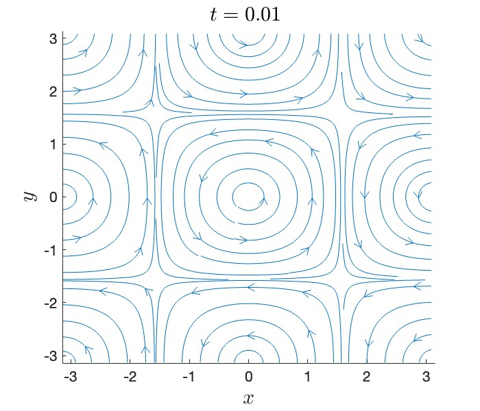
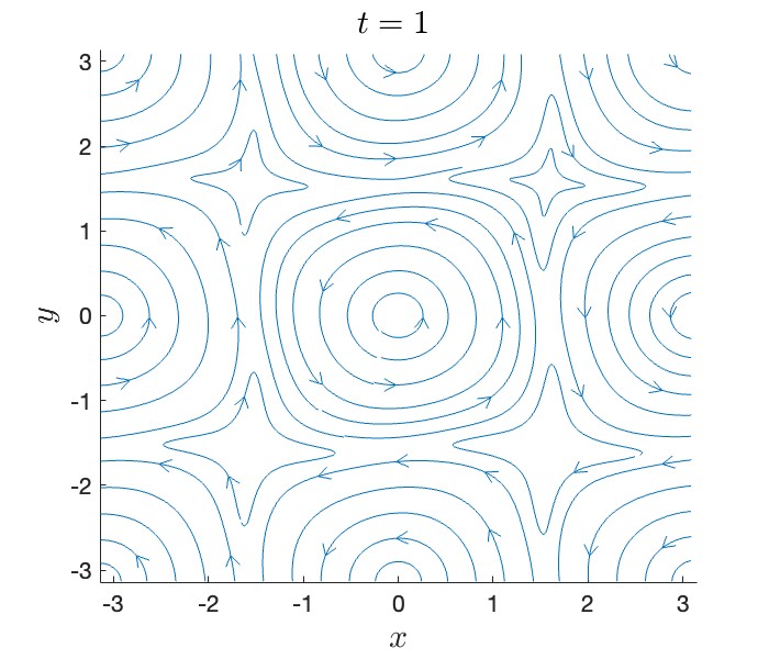
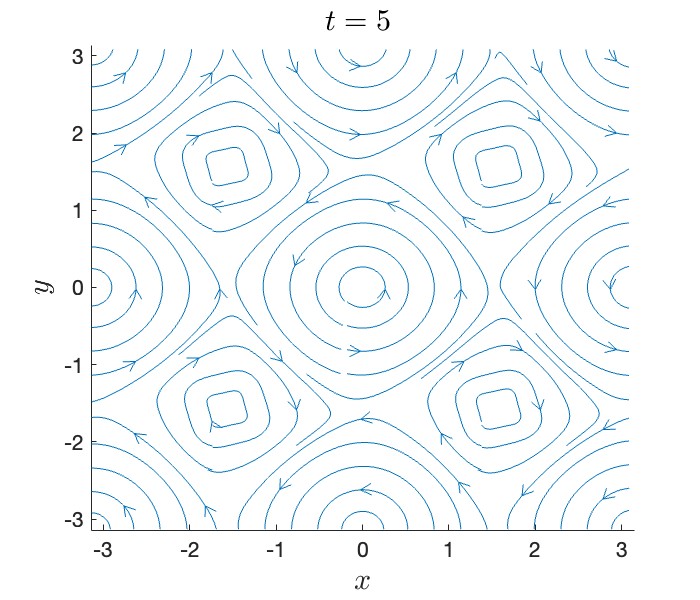
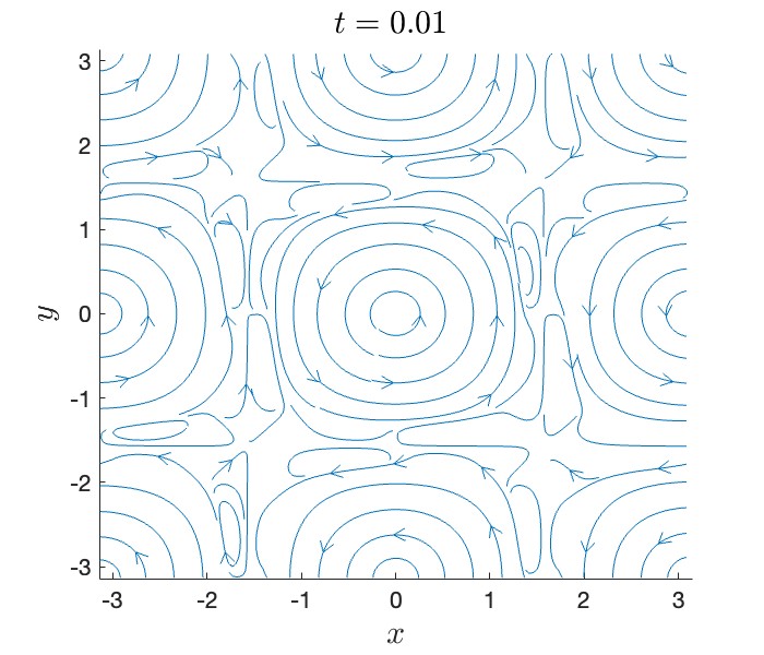
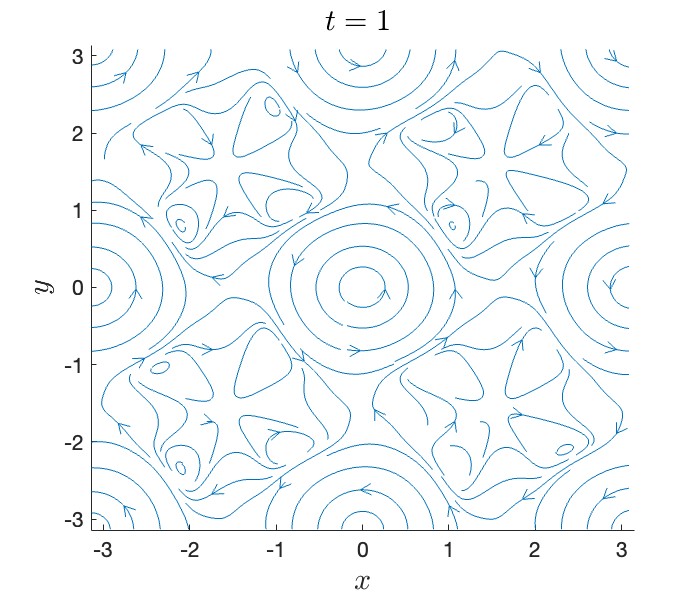
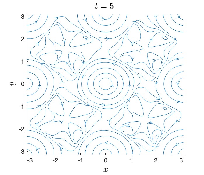
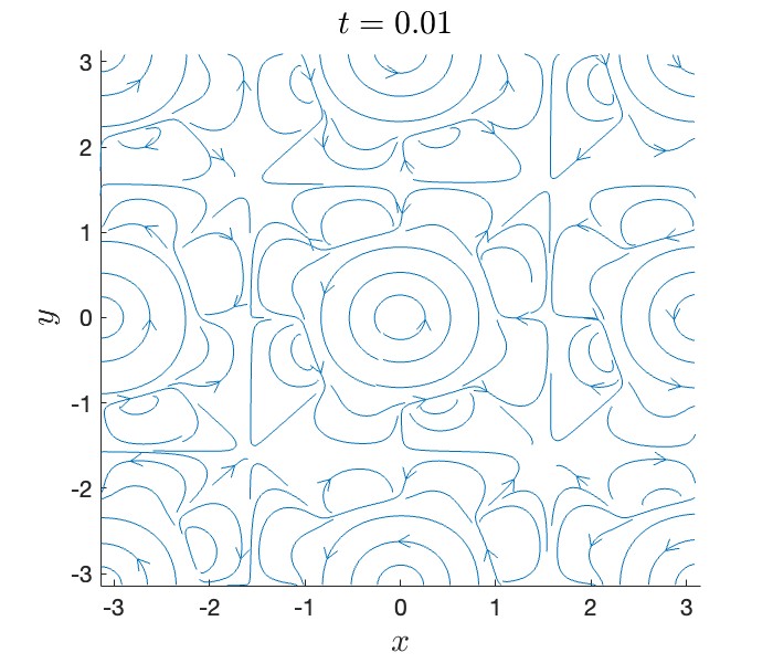
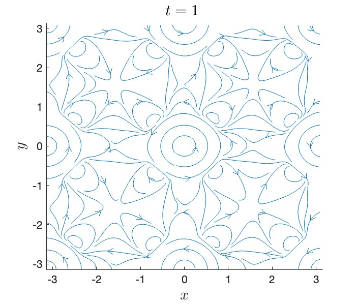
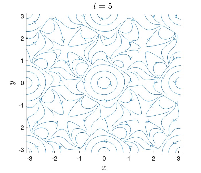
Figure 1. Dynamics of 2D incompressible Euler equations (NS equations) by scheme (5.1) where $\nu=0.0001$, $\tau=0.01,~{}N_{x}=N_{y}=128$ and the initial data $u_{0}$ is given in (6.1). $m=2$ in the first line, $m=8$ in the second line and $m=20$ in the third line.

In the second example we consider the following double shear flow initial condition:

$$w_{0}=\nabla^{\perp}\cdot\vec{u}_{0}=\begin{cases}&0.05\cos(x+\pi)-\frac{1}{\rho_{0}}\mathop{\mathrm{sech}}^{2}(\frac{1}{\rho_{0}}(y+\frac{\pi}{2})),\,y\leq 0\\ &0.05\cos(x+\pi)+\frac{1}{\rho_{0}}\mathop{\mathrm{sech}}^{2}(\frac{1}{\rho_{0}}(y-\frac{\pi}{2})),\,y>0\end{cases},$$ (6.2)

where $\rho_{0}=\frac{\pi}{15}$. We present the dynamics of the vorticity $w=\nabla^{\perp}\cdot u$ in Figure 2. Here we fix $\tau=0.001,~{}N_{x}=N_{y}=128$ and the initial data $u_{0}$ is given in (6.2). We vary the choice $\nu=0,0.001,0.1$. From the dynamics we can observe that when the Reynolds number is large (viscosity $\nu$ is small) the dynamics of the double shear flow tends to rotate and therefore to be turbulent due to the transport term $u\cdot\nabla u$. On the contrary, while the Reynolds number is small (viscosity $\nu$ is large) the dynamics of the double shear flow tends to be more stable due to the viscosity term $\nu\Delta u$.

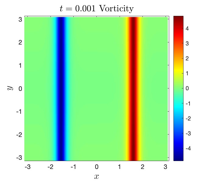
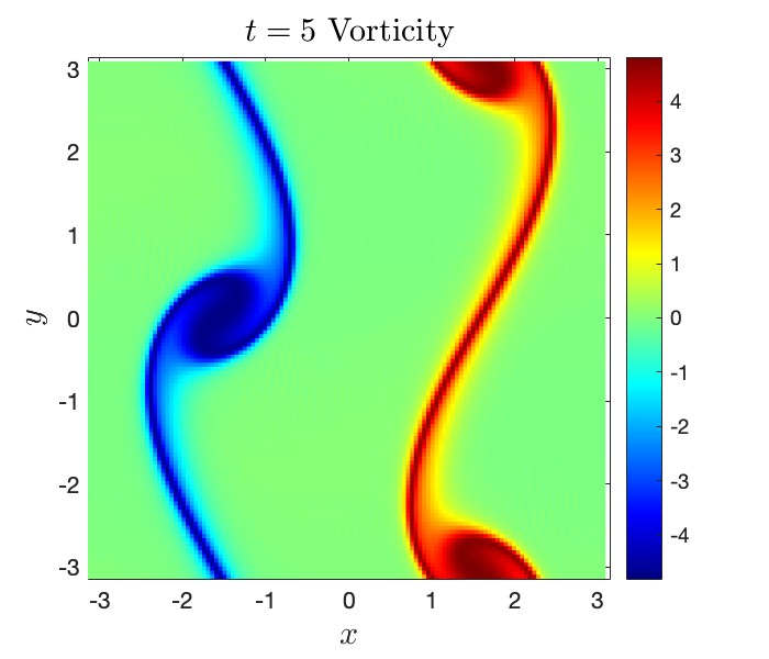
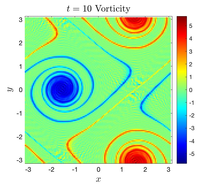
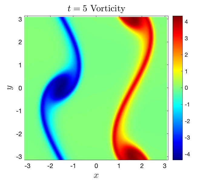
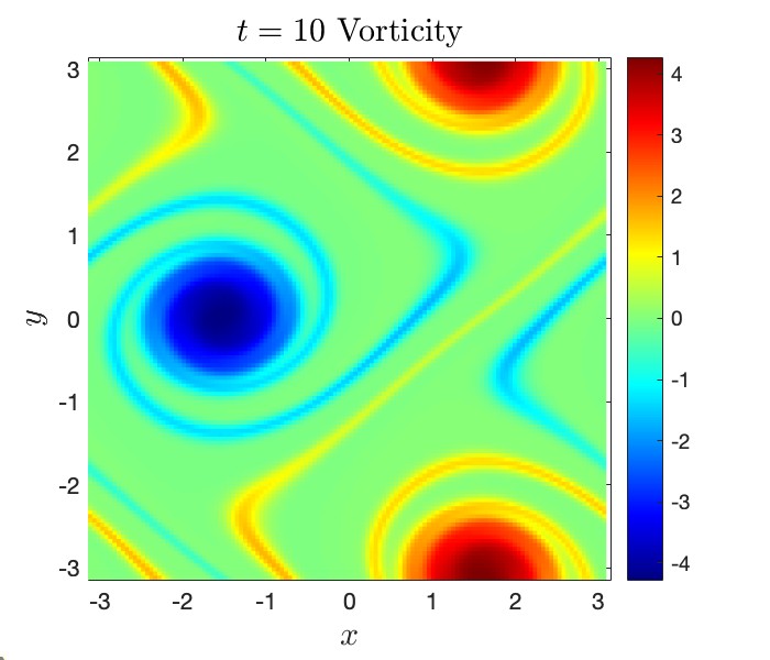
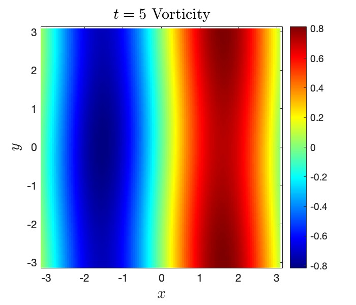
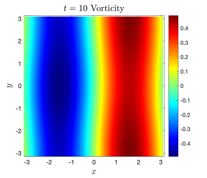
Figure 2. Dynamics of 2D incompressible Euler (NS) equations by scheme (5.1) where $\tau=0.001,~{}N_{x}=N_{y}=128$ and the initial data $u_{0}$ is a double shear flow given in (6.2). We vary the choice $\nu=0,0.001,0.1$. $\nu=0$ in the first line, $\nu=0.001$ in the second line and $\nu=0.1$ in the third line.

In the third example we consider the following initial data of two Guassian vortices. The initial vorticity is given as

$$w_{0}=\nabla^{\perp}\cdot\vec{u_{0}}=\exp(-5((x+\frac{\pi}{4})^{2}+y^{2}))+\exp(-5((x-\frac{\pi}{4})^{2}+y^{2})).$$ (6.3)

We present the dynamics of the vorticity by fixing $\tau=0.001,N_{x}=N_{y}=128$ with the initial data given in (6.3). We present the vorticity with different $\nu=0,0.001,0.1$ at $T=50$ in Figure 3. From the dynamics we can observe that when the viscosity $\nu$ is small the dynamics of the two Guassian vortices tend to merge as they orbit around each other. On the contrary, while the viscosity $\nu$ is large the dynamics tend to be more stable.

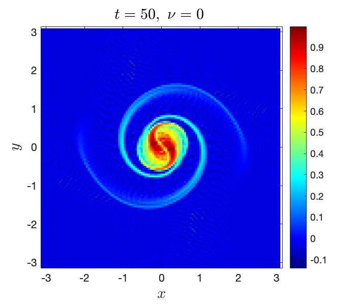
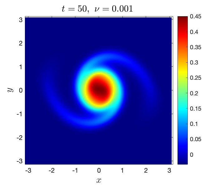
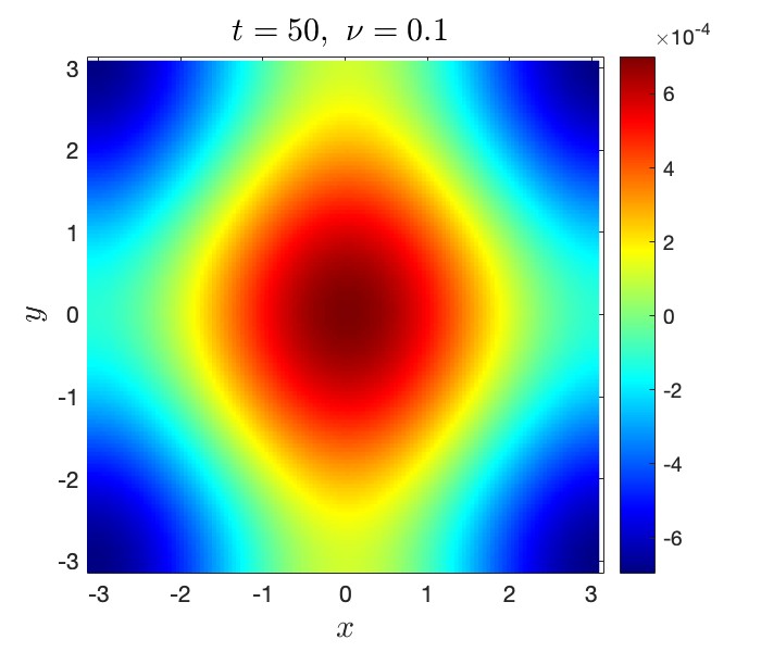
Figure 3. Dynamics of 2D incompresible Euler (NS) equations by scheme (5.1) where $\tau=0.001,~{}N_{x}=N_{y}=128$ and the initial data $u_{0}$ is composed of two Guassian vortices given in (6.3).

6.2. Convergence test

In this section we present the error of the scheme (5.1). Throughout this subsection we choose an explicit solution to the Euler equations:

$$\vec{u_{e}}=(-0.5\exp(-t)\sin(x)\cos(y),0.5\exp(-t)\cos(x)\sin(y)),$$ (6.4)

with initial data $u_{0}=(-0.5\sin(x)\cos(y),0.5\cos(x)\sin(y))$. Of course $\vec{u_{e}}$ cannot solve the exact Euler equations however it solves an Euler system with forcing term $\vec{f_{e}}$ that can be computed exactly. As a result we only need to compare the numerical solutions of the forced Euler (NS) system to the exact solution $\vec{u_{e}}$. To be more clear, the numerical solution $u_{n}$ we consider is the following

$$\frac{u^{n+1}-u^{n}}{\tau}+\Pi_{N}\mathbb{P}(u^{n}\cdot\nabla u^{n+1})=\nu\Delta u^{n+1}+f_{n},$$ (6.5)

where $f_{n}=\vec{f_{e}}(n\cdot\tau)$. Moreover to solve (6.5) we apply the iterative Fourier spectral method with forcing term:

$$\begin{cases}&\frac{u^{(m+1)}-u^{n}}{\tau}+\mathbb{P}\Pi_{N}(u^{n}\cdot\nabla u^{(m)})=\nu\Delta u^{(m+1)}+f_{n},\\ &\mathop{\rm div}u^{(m+1)}=0,\\ &u^{(0)}=u^{n},\quad u^{0}=\Pi_{N}u_{0}.\end{cases}$$ (6.6)

In the first experiment we fix $\nu=0.00001,N_{x}=N_{y}=128$ and we vary the time step $\tau=\frac{0.1}{2^{k}}$. The local residual is fixed to be 1e-10 in the iteration scheme (6.6). The $L^{\infty},L^{2},H^{1},H^{6}$-error at $T=2$ can be found below in Table 1. We see that the all the errors (of lower regularity) behave as $O(\tau)$, which follows Theorem 1.3.

$\tau=0.1$	$L^{2}$-error	$L^{\infty}$-error	$H^{1}$-error	$H^{6}$-error
$\tau$	0.0961	0.0432	0.2319	0.8654
$\tau/2$	0.0481	0.0216	0.1160	0.4326
$\tau/4$	0.0241	0.0108	0.0581	0.2165
$\tau/8$	0.0120	0.0054	0.0291	0.1084
$\tau/16$	0.0060	0.0027	0.0146	0.0544
$\tau/32$	0.0030	0.0014	0.0073	0.0274

Table 1. Errors for fixed $\nu$ and varying $\tau$.

In the second experiment, we fix $\tau=0.0001,N_{x}=N_{y}=128$ and we vary $\nu=\frac{0.1}{2^{k}}$. The local residual is fixed to be 1e-10 in the iteration scheme (6.6). The $L^{\infty},L^{2},H^{1},H^{6}$-error at $T=0.1$ can be found below in Table 2. We see that the all the errors (of lower regularity) behave as $O(\nu)$.

$\nu=0.1$	$L^{2}$-error	$L^{\infty}$-error	$H^{1}$-error	$H^{6}$-error
$\nu$	0.0418	0.0188	0.1010	0.3764
$\nu/2$	0.0210	0.0095	0.0508	0.1892
$\nu/4$	0.0105	0.0047	0.0255	0.0949
$\nu/8$	0.0053	0.0024	0.0128	0.0476
$\nu/16$	0.0026	0.0012	0.0064	0.0238
$\nu/32$	0.0013	5.9873e-04	0.0032	0.0120

Table 2. Errors for fixed $\tau$ and varying $\nu$.

In the third experiment, we present the high-regularity errors with different choice of $\nu$ and $N$. We fix $\tau=0.0001$ here. As shown in Table 3 the low regular $H^{6}$-error and $L^{\infty}$-error are very similar to Table 2, while the high regular $H^{8}$-error at $T=0.01$ behave very differently. Usually one may expect the error gets smaller as $N$ increases; however such intuition does not apply here since the high-regularity error may increase due to the $N^{2}\nu$ upper bound as in Theorem 1.3. It is also worth pointing here that $N^{2}\nu$ is only a technical upper bound and the real $H^{8}$-error may not lie in this order. Indeed as can be shown in the last column of the last table, the $H^{8}$-error is around $61$ even though $\nu=\frac{1}{2^{k}}$.

$N=64,\nu=1$	$L^{\infty}$-error	$H^{6}$-error	$H^{8}$-error
$\nu$	0.0188	0.3900	0.7366
$\nu/2$	0.0095	0.1960	0.3702
$\nu/4$	0.0047	0.0982	0.1856
$\nu/8$	0.0024	0.0492	0.0929
$\nu/16$	0.0012	0.0246	0.0465
$\nu/32$	5.9873e-04	0.0123	0.0233

$N=128,\nu=1$	$L^{\infty}$-error	$H^{6}$-error	$H^{8}$-error
$\nu$	0.0188	0.3900	0.7658
$\nu/2$	0.0095	0.1960	0.4251
$\nu/4$	0.0047	0.0982	0.2789
$\nu/8$	0.0024	0.0492	0.2267
$\nu/16$	0.0012	0.0246	0.2103
$\nu/32$	5.9873e-04	0.0123	0.2042

$N=256,\nu=1$	$L^{\infty}$-error	$H^{6}$-error	$H^{8}$-error
$\nu$	0.0188	0.3900	61.3436
$\nu/2$	0.0095	0.1960	61.3190
$\nu/4$	0.0047	0.0983	61.3073
$\nu/8$	0.0024	0.0493	61.3013
$\nu/16$	0.0012	0.0247	61.2978
$\nu/32$	5.9873e-04	0.0126	61.2932

Table 3. Errors for fixed $\tau$ and varying $\nu$.

7. Concluding remark

To conclude, we give a systematic approach on studying the incompressible Euler equations numerically by the Fourier spectral method via the vanishing viscosity limit. Another main contributions of this work is to propose a new integration by parts technique to lower the regularity requirement from $H^{4}$ to $H^{3}$ in order to perform the $L^{2}$-error estimate. Indeed, this analysis framework can be applied to more general models and higher order schemes. We leave the discussion in subsequent works.

Appendix A Extra energy dissipation of first derivative for velocity of the semi-implicit scheme

In this section we prove Corollary 1.2. Multiplying $-\Delta u^{n+1}$ to (3.2) and integrating on periodic torus $\mathbb{T}^{2}$, we obtain

$$\frac{1}{2}\|\nabla u^{n+1}\|^{2}_{L^{2}}+\frac{1}{2}\|\nabla\left(u^{n+1}-u^{n}\right)\|^{2}_{L^{2}}-\tau\langle u^{n}\cdot\nabla u^{n+1},\Delta u^{n+1}\rangle+\nu\tau\|\nabla^{2}u^{n+1}\|^{2}_{L^{2}}=\frac{1}{2}\|\nabla u^{n}\|^{2}_{L^{2}}.$$

Notice that $\int_{\mathbb{T}^{2}}(u\cdot\nabla)u\cdot\Delta udx=0$ provided $\nabla\cdot u=0$. Then we have

$$-\tau\langle u^{n}\cdot\nabla u^{n+1},\Delta u^{n+1}\rangle =\tau\langle\left(u^{n=1}-u^{n}\right)\cdot\nabla u^{n+1},\Delta u^{n+1}\rangle-\tau\langle u^{n+1}\cdot\nabla u^{n+1},\Delta u^{n+1}\rangle$$

$$=-\tau\langle\nabla\left(u^{n+1}-u^{n}\right)\cdot\nabla u^{n+1},\nabla u^{n+1}\rangle$$

$$\leq\tau\|\nabla\left(u^{n+1}-u^{n}\right)\|_{L^{2}}\|\nabla u^{n+1}\|^{2}_{L^{4}}$$

$$\leq\tau\|\nabla\left(u^{n+1}-u^{n}\right)\|_{L^{2}}\|\nabla^{2}u^{n+1}\|^{2}_{L^{2}}.$$

Besides if we require $C\tau\leq\nu$ additionally, then one can deduce from (3.2) that

$$\|\nabla\left(u^{n+1}-u^{n}\right)\|_{L^{2}} \leq\tau\|\nabla\left(u^{n}\cdot\nabla u^{n+1}\right)\|_{L^{2}}+\nu\tau\|u^{n+1}\|_{L^{\infty}_{t}\dot{H}^{3}}$$

$$\leq\tau(\|u^{n}\|_{H^{3}}+\nu)\|u^{n+1}\|_{H^{3}}$$

$$\leq C\tau$$

$$\leq\nu.$$

As a result, we can obtain an extra $\dot{H}^{1}$-energy dissipation:

$$\frac{1}{2}\|\nabla u^{n+1}\|^{2}_{L^{2}}+\frac{1}{2}\|\nabla\left(u^{n+1}-u^{n}\right)\|^{2}_{L^{2}}\leq\frac{1}{2}\|\nabla u^{n}\|^{2}_{L^{2}}.$$

Appendix B Energy estimates and vanishing viscosity limit for the Navier-Stokes equation

In this section we give an alternative proof of Lemma 2.2 for the sake of completeness. First of all for $k>2$, we investigate the $H^{k}$-estimates of the Navier-Stokes equation (1.2) for $t\in[0,T]$ as follows:

$$\|u\|^{2}_{H^{k}}+\nu\int_{0}^{t}\|\nabla u\|^{2}_{H^{k}}dt^{\prime}\leq\|u_{0}\|^{2}_{H^{k}}\exp\left(C\int_{0}^{t}\|u\|_{H^{k}}dt^{\prime}\right).$$

Taking $T=\frac{1}{4C\|u_{0}\|_{H^{k}}}$ and assuming $\|u\|_{L^{\infty}_{t}H^{k}}\leq 4\|u_{0}\|_{H^{k}}$, then we know

$$\|u\|_{H^{k}}+\left(\nu\int_{0}^{t}\|\nabla u\|^{2}_{H^{k}}dt^{\prime}\right)^{1/2}\leq\|u_{0}\|_{H^{k}}e^{1/2}\leq 2\|u_{0}\|_{H^{k}}.$$

Inductively we obtain the uniform estimates for solution on $[0,T]$

$$\|u\|_{H^{k}}\leq 2\|u_{0}\|_{H^{k}}.$$ (B.1)

One can see that the uniform estimates for the Navier-Stokes equations (1.2) is also valid for the Euler equations (1.1).

Let $w:=u-v$. By (1.2) and (1.1), we know $w$ satisfy

$$\begin{cases}&\partial_{t}w+u\cdot\nabla w+w\cdot\nabla v+\nabla(p-q)=\nu\Delta w+\nu\Delta v,\quad\nabla\cdot w=0,\\ &w|_{t=0}=0.\end{cases}$$ (B.2)

Applying Lemma 2.1 and (B.1), for $k>2$, we deduce the $H^{s}$-estimates for the solutions of (B.2) that

$$\frac{1}{2}\frac{d}{dt}\|w\|^{2}_{H^{k-2}}+\nu\|\nabla w\|^{2}_{H^{k-2}} \lesssim\|w\|^{2}_{H^{k-2}}\|u\|_{H^{k}}+\|w\|^{2}_{H^{k-2}}\|v\|_{H^{k}}+\nu\|w\|_{H^{k-2}}\|v\|_{H^{k}},$$

$$\lesssim\|w\|^{2}_{H^{k-2}}\|u_{0}\|_{H^{k}}+\nu\|w\|_{H^{k-2}}\|u_{0}\|_{H^{k}},$$

which derives the following estimates

$$\frac{d}{dt}\|w\|_{H^{k-2}}\lesssim\|w\|_{H^{k-2}}\|u_{0}\|_{H^{k}}+\nu\|u_{0}\|_{H^{k}}.$$

By Gronwall’s inequality, we get

$$\|w\|_{L^{2}}\leq\|w\|_{H^{k-2}}\leq\nu CT\|u_{0}\|_{H^{k}}\exp\left(CT\|u_{0}\|_{H^{k}}\right)\lesssim\nu.$$ (B.3)

According to the interpolation theory, for $k-2\leq k^{\prime}<k$, we know

$$\|w\|_{\dot{H}^{k^{\prime}}}\lesssim\|w\|^{\frac{k-k^{\prime}}{2}}_{\dot{H}^{k-2}}\|w\|^{1-\frac{k-k^{\prime}}{2}}_{H^{k}}\lesssim\nu^{\frac{k-k^{\prime}}{2}}\|u_{0}\|^{1-\frac{k-k^{\prime}}{2}}_{H^{k}}.$$

Then we take $u^{\sigma}_{0}:=\mathcal{F}^{-1}\left(\mathcal{I}_{|\xi|\leq\frac{1}{\sigma}}\mathcal{F}u_{0}\right)$, where $\sigma$ is sufficiently small. One can easily deduce that

$$\|u^{\sigma}_{0}\|_{H^{k}}\lesssim\|u_{0}\|_{H^{k}},$$

$$\|u^{\sigma}_{0}\|_{H^{k+1}}\lesssim\frac{1}{\sigma}\|u_{0}\|_{H^{k}},~{}~{}~{}~{}\|u^{\sigma}_{0}\|_{H^{k+2}}\lesssim\frac{1}{\sigma^{2}}\|u_{0}\|_{H^{k}},$$

$$\|u^{\sigma}_{0}-u_{0}\|_{H^{k^{\prime}}}\lesssim\sigma^{k-k^{\prime}}\|u^{\sigma}_{0}-u_{0}\|_{H^{k}}.$$

Considering the evolution equations for initial data $u^{\sigma}_{0}$, we get

$$\begin{cases}&\partial_{t}u^{\sigma}+u^{\sigma}\cdot\nabla u^{\sigma}+\nabla p^{\sigma}=\nu\Delta u^{\sigma},\quad\nabla\cdot u^{\sigma}=0,\\ &u|_{t=0}=u^{\sigma}_{0}.\end{cases}$$ (B.4)

and

$$\begin{cases}&\partial_{t}v^{\sigma}+v^{\sigma}\cdot\nabla v^{\sigma}+\nabla q^{\sigma}=0,\quad\nabla\cdot v^{\sigma}=0,\\ &u|_{t=0}=u^{\sigma}_{0}.\end{cases}$$ (B.5)

Let $l\geq k$. Similarly, we also have

$$\|u^{\sigma}\|_{H^{l}}\lesssim\|u^{\sigma}_{0}\|_{H^{l}}\lesssim\|u_{0}\|_{H^{l}},$$ (B.6)

and

$$\|v^{\sigma}\|_{H^{l}}\lesssim\|v^{\sigma}_{0}\|_{H^{l}}\lesssim\|u_{0}\|_{H^{l}}.$$ (B.7)

Let $e^{\sigma}:=u^{\sigma}-u$. By (1.2) and (B.4), we have

$$\begin{cases}&\partial_{t}e^{\sigma}+u\cdot\nabla e^{\sigma}+e^{\sigma}\cdot\nabla u^{\sigma}+\nabla(p^{\sigma}-q^{\sigma})=\nu\Delta e^{\sigma},\quad\nabla\cdot e^{\sigma}=0,\\ &e^{\sigma}|_{t=0}=u^{\sigma}_{0}-u_{0}.\end{cases}$$ (B.8)

Applying Lemma 2.1 and (B.8), we obtain

$$\frac{1}{2}\frac{d}{dt}\|e^{\sigma}\|^{2}_{H^{k-1}}+\nu\|\nabla e^{\sigma}\|^{2}_{H^{k-1}}\lesssim\|e^{\sigma}\|^{2}_{H^{k-1}}\|u\|_{H^{k}}+\|e^{\sigma}\|^{2}_{H^{k-1}}\|u^{\sigma}\|_{H^{k}},$$

which implies that

$$\frac{d}{dt}\|e^{\sigma}\|_{H^{k-1}}\lesssim\left(\|u^{\sigma}\|_{H^{k}}+\|u\|_{H^{k}}\right)\|e^{\sigma}\|_{H^{k-1}}.$$

By Gronwall’s inequality, we get

$$\|e^{\sigma}\|_{H^{k-1}} \lesssim\exp\left(CT\|u_{0}\|_{H^{k}}\right)\|e_{0}\|_{H^{k-1}}\lesssim\|e_{0}\|_{H^{k-1}}.$$

Applying Lemma 2.1 and (B.6), we deduce that

$$\frac{1}{2}\frac{d}{dt}\|e^{\sigma}\|^{2}_{H^{k}}+\nu\|\nabla e^{\sigma}\|^{2}_{H^{k}} \lesssim\|e^{\sigma}\|^{2}_{H^{k}}\|u\|_{H^{k}}+\|e^{\sigma}\|^{2}_{H^{k}}\|u^{\sigma}\|_{H^{k}}+\|u^{\sigma}\|_{H^{k+1}}\|e^{\sigma}\|_{H^{k-1}}\|e^{\sigma}\|_{H^{k}},$$

$$\lesssim\|e^{\sigma}\|^{2}_{H^{k}}\|u_{0}\|_{H^{k}}+\frac{1}{\sigma}\|u_{0}\|_{H^{k}}\|e^{\sigma}_{0}\|_{H^{k-1}}\|e^{\sigma}\|_{H^{k}}.$$

which derives the following estimates

$$\frac{d}{dt}\|e^{\sigma}\|_{H^{k}}\lesssim\|e^{\sigma}\|_{H^{k}}\|u_{0}\|_{H^{k}}+\frac{1}{\sigma}\|u_{0}\|_{H^{k}}\|e^{\sigma}_{0}\|_{H^{k-1}}.$$

By Gronwall’s inequality, we get

$$\|e^{\sigma}\|_{H^{k}} \lesssim\exp\left(CT\|u_{0}\|_{H^{k}}\right)\left(\|e^{\sigma}_{0}\|_{H^{k}}+\frac{1}{\sigma}T\|u_{0}\|_{H^{k}}\sigma\|e^{\sigma}_{0}\|_{H^{k}}\right)$$

$$\lesssim\|u^{\sigma}_{0}-u_{0}\|_{H^{k}}.$$ (B.9)

Similarly, we also have

$$\|v^{\sigma}-v\|_{H^{k}}\lesssim\|u^{\sigma}_{0}-u_{0}\|_{H^{k}}.$$ (B.10)

Let $w^{\sigma}:=u^{\sigma}-v^{\sigma}$. Using (B.4) and (B.5), we infer that

$$\begin{cases}&\partial_{t}w^{\sigma}+u^{\sigma}\cdot\nabla w^{\sigma}+w^{\sigma}\cdot\nabla v^{\sigma}+\nabla(p^{\sigma}-q^{\sigma})=\nu\Delta w^{\sigma}+\nu\Delta v^{\sigma},\quad\nabla\cdot w^{\sigma}=0,\\ &w^{\sigma}|_{t=0}=0.\end{cases}$$ (B.11)

From (B.11), then we have

$$\frac{1}{2}\frac{d}{dt}\|w^{\sigma}\|^{2}_{H^{k-1}}+\nu\|\nabla w^{\sigma}\|^{2}_{H^{k-1}} \lesssim\|w^{\sigma}\|^{2}_{H^{k-1}}\|u^{\sigma}\|_{H^{k}}+\|w^{\sigma}\|^{2}_{H^{k-1}}\|v^{\sigma}\|_{H^{k}}+\nu\|w^{\sigma}\|_{H^{k-1}}\|v^{\sigma}\|_{H^{k+1}},$$

$$\lesssim\|w\|^{2}_{H^{k-1}}\|u_{0}\|_{H^{k}}+\frac{\nu}{\sigma}\|w\|_{H^{k-1}}\|u_{0}\|_{H^{k}},$$

which derives the following estimates

$$\frac{d}{dt}\|w^{\sigma}\|_{H^{k-1}}\lesssim\|w^{\sigma}\|_{H^{k-1}}\|u_{0}\|_{H^{k}}+\frac{\nu}{\sigma}\|u_{0}\|_{H^{k}}.$$

By Gronwall’s inequality, we get

$$\|w^{\sigma}\|_{H^{k-1}} \lesssim\frac{\nu T}{\sigma}\|u_{0}\|_{H^{k}}exp\left(CT\|u_{0}\|_{H^{k}}\right)\lesssim\frac{\nu}{\sigma}.$$

Applying Lemma 2.1 again, we obtain

$$\frac{1}{2}\frac{d}{dt}\|w^{\sigma}\|^{2}_{H^{k}}+\nu\|\nabla w^{\sigma}\|^{2}_{H^{k}} \lesssim\|u^{\sigma}\|_{H^{k}}\|w^{\sigma}\|^{2}_{H^{k}}+\|v^{\sigma}\|_{H^{k}}\|w^{\sigma}\|^{2}_{H^{k}}$$

$$\quad+\|w^{\sigma}\|_{H^{k-1}}\|v^{\sigma}\|_{H^{k+1}}\|w^{\sigma}\|_{H^{k}}+\|v^{\sigma}\|_{H^{k+2}}\|w^{\sigma}\|_{H^{k}}.$$

This together with (B.7) implies that

$$\frac{d}{dt}\|w^{\sigma}\|_{H^{k}} \lesssim\|u^{\sigma}\|_{H^{k}}\|w^{\sigma}\|_{H^{k}}+\|v^{\sigma}\|_{H^{k}}\|w^{\sigma}\|_{H^{k}}$$

$$\quad+\|w^{\sigma}\|_{H^{k-1}}\|v^{\sigma}\|_{H^{k+1}}+\nu\|v^{\sigma}\|_{H^{k+2}}$$

$$\lesssim\|u_{0}\|_{H^{k}}\|w^{\sigma}\|_{H^{k}}+\frac{\nu}{\sigma^{2}}\|u_{0}\|_{H^{k}}$$

By Gronwall’s inequality, we get

$$\|w^{\sigma}\|_{H^{k}}\lesssim\exp\left(CT\|u_{0}\|_{H^{k}}\right)T\|u_{0}\|_{H^{k}}\frac{\nu}{\sigma^{2}}\lesssim\frac{\nu}{\sigma^{2}}.$$ (B.12)

Combining (B), (B.10) and (B.12), we infer that

$$\|w\|_{H^{k}} \lesssim\|e^{\sigma}\|_{H^{k}}+\|v^{\sigma}-v\|_{H^{k}}+\|w^{\sigma}\|_{H^{k}}$$

$$\lesssim\|u^{\sigma}_{0}-u_{0}\|_{H^{k}}+\frac{\nu}{\sigma^{2}}.$$

In particular by taking $\sigma=\frac{1}{N}$ we can obtain that

$$\|w\|_{H^{k}} \lesssim\|\Pi_{N}e\|_{H^{k}}+\|\Pi_{N}v-v\|_{H^{k}}+\|\Pi_{N}w\|_{H^{k}}$$

$$\lesssim\|\Pi_{N}u_{0}-u_{0}\|_{H^{k}}+N^{2}\nu.$$ (B.13)

References

- [1] D. Albritton, E. Brué and M. Colombo. Non-uniqueness of Leray solutions of the forced Navier-Stokes equations. Annals of Mathematics, 196(1): 415-455, 2022.
- [2] H. Bahouri, J. Y. Chemin and R. Danchin. Fourier analysis and nonlinear partial differential equations, Springer, Heidelberg, 2011.
- [3] G. Bai, B. Li and Y. Wu. A constructive low-regularity integrator for the 1d cubic nonlinear Schrödinger equation under the Neumann boundary condition. IMA J. Numer. Anal., 43(6): 3243–3281, 2023.
- [4] J. T. Beale, T. Kato and A. Majda. Remarks on the Breakdown of Smooth Solutions for the 3D Euler Equations. Comm. Math. Phys., 94(1):61–66 1984.
- [5] J. Bourgain, D. Li. Strong ill-posedness of the Incompressible Euler Equation in Borderline Sobolev Spaces. Invent. Math., 201(1):97–157, 2015.
- [6] J. Bourgain and N. Pavlovic. Ill-posedness of the Navier-Stokes Equations in a Critical Space in 3D. J. Funct. Anal., 255(9):2233–2247 2008.
- [7] T. Buckmaster, S. Shkoller and V. Vicol. Nonuniqueness of weak solutions to the SQG equation. Commun. Pure Appl. Math., 72(9): 1809–1874, 2019.
- [8] X. Cheng, H. Kwon and D. Li. Non-uniqueness of stationary weak solutions to the surface quasi-geostrophic equations. Comm. Math. Phys., 388 (3): 1281-1295, 2021.
- [9] A.J. Chorin. Numerical solution of the Navier–Stokes equations. Math. Comput., 22, 745–762, 1968.
- [10] A.J. Chorin. On the convergence of discrete approximations to the Navier–Stokes equations. Math. Comput., 23, 341–353, 1969.
- [11] P. Constantin, T. D. Drivas, T. M. Elgindi. Inviscid Limit of Vorticity Distributions in the Yudovich Class. Comm. Pure Appl. Math., 75(1):60–82, 2022.
- [12] C. De Lellis and L. Székelyhidi, Jr. Dissipative continuous Euler flows. Invent. Math., 193(2): 377–407, 2013.
- [13] W. E and J. Liu. Projection method I: convergence and numerical boundary layers. SIAM journal on numerical analysis, 1017-1057, 1995.
- [14] W. E and J. Liu. Projection method III: spatial discretization on the staggered grid[J]. Mathematics of computation, 71(237): 27-47, 2002.
- [15] T. Elgindi. Finite-time Singularity Formation for Solutions to the Incompressible Euler Equations on . Ann. of Math. (2), 2021, 194(3):647–727.
- [16] H. Fujita, T. Kato. On the Navier-Stokes Initial Value Problem I. Arch. Rational Mech. Anal., 16:269–315, 1964.
- [17] B. Guo and J. Zou. Fourier spectral projection method and nonlinear convergence analysis for Navier–Stokes equations. Journal of mathematical analysis and applications, 282(2): 766-791, 2003.
- [18] Z. Guo, J. Li and Z. Yin. Local Well-posedness of the Incompressible Euler Equations in and the Inviscid Limit of the Navier-Stokes Equations. J. Funct. Anal., 276(9): 2821–2830, 2019.
- [19] A. Hakim. SimJournal: Ammar Hakim’s Simulation Journal (2022), https://ammar-hakim.org/sj/index.html.
- [20] Y. He. Euler implicit/explicit iterative scheme for the stationary Navier–Stokes equations. Numer. Math., 123, 67–96, 2013.
- [21] J.G. Heywood and R. Rannacher. Finite element approximation of the nonstationary Navier–Stokes problem. I. Regularity of solutions and second-order spatial discretization. SIAM J. Numer. Anal., 19, 275–311, 1982.
- [22] J.G. Heywood and R. Rannacher. Finite-element approximation of the nonstationary Navier–Stokes problem part IV: error analysis for second-order time discretization. SIAM J. Numer. Anal., 27, 353–384, 1990.
- [23] T. Y. Hou and B. Wetton. Second-Order Convergence of a Projection Scheme for the Incompressible Navier–Stokes Equations with Boundaries, SIAM Journal on Numerical Analysis, 30(3): 609–629, 1993.
- [24] P. Isett. A proof of Onsager’s conjecture, Ann. of Math., 188(3): 871–963, 2018.
- [25] A. Kiselev, V. Sverak. Small Scale Creation for Solutions of the Incompressible Two-dimensional Euler Equation. Ann. of Math. (2), 180(3):1205–1220, 2014.
- [26] J. Leray. Sur Le Mouvement Dun Liquide Visqueux Emplissant Lespace. Acta Math., 63(1):193–248, 1934.
- [27] Z. Lei and F. Lin. Global mild solutions of Navier–Stokes equations. Communications on Pure and Applied Mathematics, 64(9): 1297-1304, 2011.
- [28] B. Li. A bounded numerical solution with a small mesh size implies existence of a smooth solution to the Navier–Stokes equations.Numerische Mathematik, 147(2): 283-304, 2021.
- [29] B. Li, S. Ma and K. Schratz. A Semi-implicit Exponential Low-Regularity Integrator for the Navier–Stokes Equations. SIAM J. Numer. Anal., 60(4): 2273-2292, 2022.
- [30] X. Luo. Stationary solutions and nonuniqueness of weak solutions for the Navier–Stokes equations in high dimensions. Arch. Ration. Mech. Anal., 233: 701–747, 2019.
- [31] N. Masmoudi, Remarks about the inviscid limit of the Navier-Stokes system, Commun. Math. Phys., 270(3): 777–788, 2007.
- [32] N. Masmoudi, F. Rousset. Uniform regularity for the Navier–Stokes equation with Navier boundary condition. Archive for Rational Mechanics and Analysis, 203: 529-575, 2012.
- [33] F. Rousset and K. Schratz. A general framework of low regularity integrators, SIAM J. Numer. Anal., 59(3): 1735–1768, 2021.
- [34] E. Süli. Convergence and non-linear stability of the Lagrange–Galerkin method for the Navier–Stokes equations. Numer. Math., 53, 459–483, 1988.
- [35] X. Wang. An efficient second order in time scheme for approximating long time statistical properties of the two dimensional Navier–Stokes equations. Numer. Math., 121: 753–779, 2012.
- [36] Y. Wu and X. Zhao. Optimal convergence of a second order low-regularity integrator for the KdV equation. IMA J. Numer. Anal., 42(4): 3499–3528, 2022.
- [37] V. I. Yudovich. Non-stationary Flows of an Ideal Incompressible Fluid. Z. Vycisl. Mat i Mat. Fiz., 3:1032–1066, 1963.