Riemann problem for Aw-Rascle model with more realistic version of extended Chaplygin gas

Abstract.

The motivation of this study is to find the Riemann solutions of Aw-Rascle model with friction for a more realistic version of extended Chaplygin gas. Firstly, we established the $\delta$-shock wave in its solutions; indeed, by using generalized Rankine Hugoniot jump conditions the position, strength, and velocity of $\delta$-shock are obtained. Further, by analyzing the limiting behavior, it is found that one of the Riemann solutions converges to $\delta$-shock solution as the pressure approaches to generalized Chaplygin gas pressure. Moreover, we obtained that our Riemann solutions converge to the corresponding solutions of the transport equations as pressure tends to zero. Furthermore, we explicitly construct the Riemann solutions of the inhomogeneous Aw-Rascle model.

Keywords. Riemann problem, Chaplygin gas, Delta shock, Aw-Rascle model, Transport equations, Coulomb like friction

1. introduction

In Recent times, the Aw-Rascle model has drawn a lot of attention due to its physical significance, such as the dynamics and formation of traffic jams. In the related research on this model, the appearance of $\delta$-shock waves in its solutions has become an interesting topic for many researchers [1, 8, 21, 22, 27, 25, 23]. Unlike the ordinary shock, $\delta$-shock is an over-compressive shock in which more characteristics impinge to the line of discontinuity. Physically, the $\delta$-shock wave demonstrates that the speed of the cars ahead is considerably slower than that of the cars behind, which results in serious jams.
            The conservative form of the Aw-Rascle model is given by [1]

$$\begin{cases}\rho_{t}+(\rho u)_{x}=0,\\ (\rho(u+p))_{t}+(\rho u(u+p))_{x}=0,\end{cases}$$ (1)

where $\rho>0$, $u$ $\geq$ 0, and $p$ stand for traffic density, velocity, and pressure, respectively. The velocity of traffic is always non-negative. Unlike a fluid particle that responds to both frontal and backward stimuli, a car responds to frontal stimuli only due to its anisotropic nature. Also, the pressure function $p=p(\rho)$ in traffic flow is the offset velocity, commonly known as the pressure inspired by the gas dynamics; indeed, it serves as an anticipation factor reflecting the responses of the drivers to the scenario of traffic ahead of them. In 2000, Aw and Rascle [1] proposed the model (1) to overcome the shortcomings of the second order models of car traffic identified by Daganzo [9]. This model had also been independently drawn by Zhang [40]. In 2012, Pan and Han [22] studied the model (1) with Chaplygin pressure and obtained that the Riemann solutions of (1) coincide with the Riemann solutions of pressureless gas dynamics when the traffic pressure drops to zero. Cheng and Yang [8] discussed the Riemann problem for system (1) and showed the occurrence of $\delta$-shock in its solutions as pressure converges to Chaplygin pressure. Shen and Sun [27] analyzed the appearance of $\delta$-shock and vacuum states in the perturbed Aw-Rascle model. In 2013, Cheng [5, 7] showed that the Riemann solutions to Chaplygin nonsymmetric Keyfitz-Kranzer type system were very similar to the corresponding Chaplygin Aw-Rascle model.
            As the traffic pressure falls to zero, the model (1) converts into the following transport equations [3, 11]

$$\begin{cases}\rho_{t}+(\rho u)_{x}=0,\\ (\rho u)_{t}+(\rho u^{2})_{x}=0,\end{cases}$$ (2)

which describe the motion of free particles stick under collision. Since 1994, numerous researchers have extensively studied the transport equations [15, 11, 29, 32, 33, 19, 6, 37, 17, 20, 34, 28, 39]; in particular, E, Rykov and Sinai [11] investigated the behavior of global weak solution to $1$-D Riemann problem with random initial data. With the use of vanishing viscosity and characteristic analysis method, Sheng and Zhang [29] studied the solutions of $1$-D and $2$-D Riemann problems. Li and Yang [19] examined $1$-D Riemann problem and obtained multidimensional planar delta shock waves depending on one-parameter family. Jiang et al. [16] constructed the Riemann solutions of non-isentropic improved Aw-Rascle-Zhang model with delta initial data and studied the interactions of elementary waves with $\delta$-shock waves. Further, Shao and Huang [24] discussed the $\delta$-shocks interactions in the Riemann solutions of system (1) when initial data consist three piece-wise constant states.
            The Aw-Rascle model with coulomb like friction is stated as [21]

$$\begin{cases}\rho_{t}+(\rho u)_{x}=0,\\ (\rho(u+p))_{t}+(\rho u(u+p))_{x}=\eta\rho,\end{cases}$$ (3)

where $\rho>0$, $u$ $\geq 0,$ $p,$ and $\eta$ stand for traffic density, velocity, pressure, and frictional constant, respectively. Yin and Chen [38] investigated the Riemann problem along with the stability of Riemann solutions to the system (3). Zhang [41] explicitly solved the Riemann problem of system (3) with Chaplygin pressure and precisely investigated the vanishing pressure limit of its Riemann solutions. Moreover, Li [21] obtained the Riemann solutions of system (3) with anti-Chaplygin pressure and determined that the solutions lose their self-similarity nature due to the presence of friction term. The more realistic version of extended Chaplygin gas is described by the following equation of state [2]

$$p=A\left(\frac{\rho}{1-a\rho}\right)^{\Gamma}-\frac{B}{\rho^{\kappa}},\quad(1\leq\Gamma\leq 3,\,0<\kappa\leq 1),$$ (4)

where $A>0$ and $B>0$ are constants; $a$ represents the van der Waals excluded volume. In particular, for $A=0$ and $\kappa=1,$ the model (4) reduces to Chaplygin gas model $P=-B/\rho;$ it is considered aerodynamically reasonable mathematical approximation for estimating wing’s lift [4, 35, 36].

As we have seen above different exotic pressure laws to some extent embody the internal mechanism of solutions to Aw-Rascle traffic flow model. In fact, it is crucial to consider Aw-Rascle model with several pressure laws. From a physical perspective, Aw-Rascle model is one of the vital fluid dynamics model for traffic flow [9, 1]. Hence, it is feasible to characterize some peculiar traffic phenomena using various exotic equations of state, viz., Polytropic gas, Chaplygin gas, extended Chaplygin gas etc. While from a mathematical perspective, different pressure laws have a significant impact on the traffic flow model’s solutions. More significantly, some odd phenomena are analyzed by the researchers in the traffic flow model’s solutions with these pressure laws. One of such phenomenon is observed by Shen and Sun in their paper [27], they found that their Riemann solutions do not converge to the Riemann solutions of transport equations, whenever, the traffic pressure drops to zero. Recently, Fan and Zhang [13, 14] studied the Riemann solutions in Aw-Rascle model with modified and extended Chaplygin gases.
            Motivating from these, in the current study, we consider the system (3)-(4) with the following initial data

$$(\rho,u)_{t=0}=\begin{cases}(\rho_{l},u_{l}),\quad x<0,\\ (\rho_{r},u_{r}),\quad x>0.\end{cases}$$ (5)

The primary objective of this work is to investigate the existence and uniqueness of the Riemann solutions to system (3)-(4) with (5). Indeed, the formation of different kinds of $\delta$-shock waves has been shown when the initial data lie in a specific domain. Using the method of characteristic analysis, we construct the Riemann solutions with two different structures, viz., $S+J$ and $R+J$, whenever $\upsilon_{r}>-A\left(\frac{-1}{a}\right)^{\Gamma}+\upsilon_{l}+A\left(\frac{\rho_{l}}{1-a\rho_{l}}\right)^{\Gamma}-\frac{B}{\rho_{l}^{\kappa}}$. However, for $\upsilon_{r}\leqslant-A\left(\frac{-1}{a}\right)^{\Gamma}+\upsilon_{l}+A\left(\frac{\rho_{l}}{1-a\rho_{l}}\right)^{\Gamma}-\frac{B}{\rho_{l}^{\kappa}},$ we establish that Riemann solution can not be constructed by $S+J$ or $R+J$, implying thereby that $\delta$-shock should occur. Further, we obtained that the Riemann solution $S+J$ converges to $\delta$-shock solution whenever, $-A\left(\frac{-1}{a}\right)^{\Gamma}+\upsilon_{l}+A\left(\frac{\rho_{l}}{1-a\rho_{l}}\right)^{\Gamma}-\frac{B}{\rho_{l}^{\kappa}}<\upsilon_{r}\leqslant\upsilon_{l}-\frac{B}{\rho_{l}^{\kappa}}$ and $a,A\to 0.$ Also, numerical simulations are done to check the validity of the process of formation of $\delta$-shock in the case $-A\left(\frac{-1}{a}\right)^{\Gamma}+\upsilon_{l}+A\left(\frac{\rho_{l}}{1-a\rho_{l}}\right)^{\Gamma}-\frac{B}{\rho_{l}^{\kappa}}<\upsilon_{r}\leqslant\upsilon_{l}-\frac{B}{\rho_{l}^{\kappa}}$ with $a,A\to 0.$ Moreover, it is shown that the Riemann solutions converge to the corresponding Riemann solutions of the transport equations with the same friction term as $a,A,B\to 0.$

The organization of this paper is as follows. In sections $2$ and $3,$ we find the solutions including $\delta-$shock to the Riemann problem governed by the system (3)-(4) with (5). Moreover, in section $4,$ we obtain that our Riemann solutions coincide with the solutions of transport equations as $a,A,B\to 0$. In section-5, we construct the Riemann solutions of the problem (3)-(5); indeed, the generalized Rankine-Hugoniot jump conditions are provided. Moreover, it is proved that the delta shock wave is the weak solution of the Riemann problem (3)-(5) in the distributional sense.

2. Riemann Solutions for the realistic Chaplygin Aw-Rascle model

Here, we define a new velocity variable $\upsilon(x,t)=u(x,t)-\eta t,$ [41, 12] to determine the solutions of the Riemann problem represented by (3)-(5). Under this transformation, the system (3) with (4) converts into the following conservative system:

$$\begin{cases}\rho_{t}+(\rho(\upsilon+\eta t))_{x}=0,\vspace{0.3cm}\\ \left(\rho\left(\upsilon+A\left(\frac{\rho}{1-a\rho}\right)^{\Gamma}-\frac{B}{\rho^{\kappa}}\right)\right)_{t}+\left(\rho(\upsilon+\eta t)\left(\upsilon+A\left(\frac{\rho}{1-a\rho}\right)^{\Gamma}-\frac{B}{\rho^{\kappa}}\right)\right)_{x}=0.\end{cases}$$ (6)

Now, the Riemann solutions of the original problem (3)-(5) can be obtained by system (6) with the initial data

$$(\rho,\upsilon)_{t=0}=\begin{cases}(\rho_{l},u_{l}),\,\quad x<0,\\ (\rho_{r},u_{r}),\quad x>0.\end{cases}$$ (7)

For convenience, we take $u_{l}=\upsilon_{l}$ and $u_{r}=\upsilon_{r},$ from now on (as $\upsilon(x,0)=u(x,0)$). The matrix form, for system (6), can be represent as

$$\begin{bmatrix}\rho\\ \upsilon\end{bmatrix}_{t}+\begin{bmatrix}\upsilon+\eta t&\rho\vspace{0.3cm}\\ 0&\upsilon+\eta t-\frac{\Gamma A\rho^{\Gamma}}{(1-a\rho)^{\Gamma+1}}-\frac{\kappa B}{\rho^{\kappa}}\end{bmatrix}\begin{bmatrix}\rho\\ \upsilon\end{bmatrix}_{x}=0.$$ (8)

The system (8) has the following eigenvalues and eigenvectors

$$\lambda_{1}=\upsilon+\eta t-\frac{\Gamma A\rho^{\Gamma}}{(1-a\rho)^{\Gamma+1}}-\frac{\kappa B}{\rho^{\kappa}},\bm{\overrightarrow{r_{1}}}=\left(1,-\frac{\Gamma A\rho^{\Gamma-1}}{(1-a\rho)^{\Gamma+1}}-\frac{\kappa B}{\rho^{\kappa+1}}\right)^{T},\,\lambda_{2}=\upsilon+\eta t,\,\bm{\overrightarrow{r_{2}}}=(1,0)^{T},$$

satisfying

$$\bigtriangledown\lambda_{1}\cdot\bm{\overrightarrow{r_{1}}}=-\frac{(\Gamma^{2}+\Gamma)A\rho^{\Gamma-1}}{(1-a\rho)^{\Gamma+2}}+\frac{(\kappa^{2}-\kappa)B}{\rho^{\kappa+1}}<0\,\text{and}\,\bigtriangledown\lambda_{2}\cdot\bm{\overrightarrow{r_{2}}}=0.$$

Thus, the wave associated with $\lambda_{1}$ is either shock or rarefaction wave and the wave associated with $\lambda_{2}$ is a contact discontinuity.

2.1. Rarefaction wave and contact discontinuity:

Under the self-similar transformation $\zeta=x/t,$ the Riemann problem presented by (6)-(7) transforms into the following:

$$\begin{cases}-\zeta\rho_{\zeta}+(\rho(\upsilon+\eta t))_{\zeta}=0,\vspace{0.3cm}\\ -\zeta\left(\rho\left(\upsilon+A\left(\frac{\rho}{1-a\rho}\right)^{\Gamma}-\frac{B}{\rho^{\kappa}}\right)\right)_{\zeta}+\left(\rho(\upsilon+\eta t)\left(\upsilon+A\left(\frac{\rho}{1-a\rho}\right)^{\Gamma}-\frac{B}{\rho^{\kappa}}\right)\right)_{\zeta}=0,\end{cases}$$ (9)

and

$$(\rho,\upsilon)=\begin{cases}(\rho_{l},\upsilon_{l}),\,\quad\zeta=-\infty,\\ (\rho_{r},\upsilon_{r}),\quad\zeta=+\infty.\end{cases}$$ (10)

For any smooth solution, the system (9) in simplified form can be written as

$$\begin{bmatrix}\upsilon+\eta t-\zeta&\rho\vspace{0.3cm}\\ 0&\upsilon+\eta t-\frac{\Gamma A\rho^{\Gamma}}{(1-a\rho)^{\Gamma+1}}-\frac{\kappa B}{\rho^{\kappa}}-\zeta\end{bmatrix}\begin{bmatrix}\rho_{\zeta}\\ \upsilon_{\zeta}\end{bmatrix}=0.$$ (11)

Besides, the constant state $(\rho,\upsilon)(\zeta)=\text{constant}(\rho>0),$ we have the singular solution, i.e., the contact discontinuity

$$J:\begin{cases}\zeta=\lambda_{2}=\upsilon+\eta t,\\ \upsilon=\upsilon_{l},\end{cases}$$ (12)

or the rarefaction wave

$$R:\begin{cases}\zeta=\lambda_{1}=\upsilon+\eta t-\frac{\Gamma A\rho^{\Gamma}}{(1-a\rho)^{\Gamma+1}}-\frac{\kappa B}{\rho^{\kappa}},\qquad\rho<\rho_{l},\vspace{0.3cm}\\ \frac{\upsilon-\upsilon_{l}}{\rho_{l}-\rho}=\frac{A[(\rho(1-a\rho_{l}))^{\Gamma-1}+(\rho(1-a\rho_{l}))^{\Gamma-2}(\rho_{l}(1-a\rho))+\cdots+(\rho_{l}(1-a\rho))^{\Gamma-1}]}{(1-a\rho)^{\Gamma}(1-a\rho_{l})^{\Gamma}}+\frac{B(\rho^{\kappa}-\rho_{l}^{\kappa})}{\rho^{\kappa}\rho_{l}^{\kappa}(\rho-\rho_{l})},\end{cases}$$ (13)

along with $\frac{d\lambda_{1}}{d\rho}=-\frac{(\Gamma^{2}+\Gamma)A\rho^{\Gamma-1}}{(1-a\rho)^{\Gamma+2}}+\frac{(\kappa^{2}-\kappa)B}{\rho^{\kappa+1}}<0.$

2.2. Shock wave

For a bounded discontinuity at $x=x(t),$ the following Rankine-Hugoniot jump relations hold:

$$\begin{cases}-\sigma(t)[\rho]+[\rho(\upsilon+\eta t)]=0\vspace{0.3cm},\\ -\sigma(t)\left[\rho\left(\upsilon+A\left(\frac{\rho}{1-a\rho}\right)^{\Gamma}-\frac{B}{\rho^{\kappa}}\right)\right]+\left[\rho(\upsilon+\eta t)\left(\upsilon+A\left(\frac{\rho}{1-a\rho}\right)^{\Gamma}-\frac{B}{\rho^{\kappa}}\right)\right]=0,\end{cases}$$ (14)

where $[\rho]=\rho_{l}-\rho,$ and $\sigma(t)=x^{\prime}(t),$ etc. After simplifying system of equations (14), we get the following discontinuities:
(i) Shock wave (discontinuity associated with $\lambda_{1}$)

$$S:\begin{cases}\sigma(t)=\upsilon_{l}+\eta t-\rho\left(\frac{A[(\rho(1-a\rho_{l}))^{\Gamma-1}+(\rho(1-a\rho_{l}))^{\Gamma-2}(\rho_{l}(1-a\rho))+\cdots+(\rho_{l}(1-a\rho))^{\Gamma-1}]}{(1-a\rho)^{\Gamma}(1-a\rho_{l})^{\Gamma}}+\frac{B(\rho^{\kappa}-\rho_{l}^{\kappa})}{\rho^{\kappa}\rho_{l}^{\kappa}(\rho-\rho_{l})}\right)\vspace{0.3cm}\\ \hskip 22.76228pt\vspace{0.3cm}=\upsilon+\eta t-\rho_{l}\left(\frac{A[(\rho(1-a\rho_{l}))^{\Gamma-1}+(\rho(1-a\rho_{l}))^{\Gamma-2}(\rho_{l}(1-a\rho))+\cdots+(\rho_{l}(1-a\rho))^{\Gamma-1}]}{(1-a\rho)^{\Gamma}(1-a\rho_{l})^{\Gamma}}+\frac{B(\rho^{\kappa}-\rho_{l}^{\kappa})}{\rho^{\kappa}\rho_{l}^{\kappa}(\rho-\rho_{l})}\right),\\ \frac{\upsilon-\upsilon_{l}}{\rho_{l}-\rho}=\frac{A[(\rho(1-a\rho_{l}))^{\Gamma-1}+(\rho(1-a\rho_{l}))^{\Gamma-2}(\rho_{l}(1-a\rho))+\cdots+(\rho_{l}(1-a\rho))^{\Gamma-1}]}{(1-a\rho)^{\Gamma}(1-a\rho_{l})^{\Gamma}}+\frac{B(\rho^{\kappa}-\rho_{l}^{\kappa})}{\rho^{\kappa}\rho_{l}^{\kappa}(\rho-\rho_{l})}.\end{cases}$$ (15)

(ii) Contact discontinuity (discontinuity associated with $\lambda_{2}$)

$$J:\begin{cases}\sigma(t)=\upsilon+\eta t,\\ \upsilon=\upsilon_{l}.\end{cases}$$ (16)

In view of the Lax-entropy conditions for shock curve, $\lambda_{1}(\rho,\upsilon)<\sigma(t)<\lambda_{2}(\rho,\upsilon),\,\,\lambda_{1}(\rho,\upsilon)<\sigma(t)<\lambda_{1}(\rho_{l},\upsilon_{l}),$ we have $\rho>\rho_{l},$ which, in turn, allows us to write the following

$$S:\begin{cases}\sigma(t)=\upsilon_{l}+\eta t-\rho\left(\frac{A[(\rho(1-a\rho_{l}))^{\Gamma-1}+(\rho(1-a\rho_{l}))^{\Gamma-2}(\rho_{l}(1-a\rho))+\cdots+(\rho_{l}(1-a\rho))^{\Gamma-1}]}{(1-a\rho)^{\Gamma}(1-a\rho_{l})^{\Gamma}}+\frac{B(\rho^{\kappa}-\rho_{l}^{\kappa})}{\rho^{\kappa}\rho_{l}^{\kappa}(\rho-\rho_{l})}\right)\vspace{0.3cm}\\ \hskip 22.76228pt\vspace{0.3cm}=\upsilon+\eta t-\rho_{l}\left(\frac{A[(\rho(1-a\rho_{l}))^{\Gamma-1}+(\rho(1-a\rho_{l}))^{\Gamma-2}(\rho_{l}(1-a\rho))+\cdots+(\rho_{l}(1-a\rho))^{\Gamma-1}]}{(1-a\rho)^{\Gamma}(1-a\rho_{l})^{\Gamma}}+\frac{B(\rho^{\kappa}-\rho_{l}^{\kappa})}{\rho^{\kappa}\rho_{l}^{\kappa}(\rho-\rho_{l})}\right),\\ \frac{\upsilon-\upsilon_{l}}{\rho_{l}-\rho}=\frac{A[(\rho(1-a\rho_{l}))^{\Gamma-1}+(\rho(1-a\rho_{l}))^{\Gamma-2}(\rho_{l}(1-a\rho))+\cdots+(\rho_{l}(1-a\rho))^{\Gamma-1}]}{(1-a\rho)^{\Gamma}(1-a\rho_{l})^{\Gamma}}+\frac{B(\rho^{\kappa}-\rho_{l}^{\kappa})}{\rho^{\kappa}\rho_{l}^{\kappa}(\rho-\rho_{l})},\quad\rho>\rho_{l}.\end{cases}$$ (17)

Also, it may be observed that the shock and rarefaction wave curves have the same expression. Indeed, we have

$$\upsilon_{\rho}=-\frac{\Gamma A\rho^{\Gamma-1}}{(1-a\rho)^{\Gamma+1}}-\frac{\kappa B}{\rho^{\kappa+1}}=-p_{\rho}<0,$$ (18)

implying thereby that, in respect of $\rho,$ the shock and rarefaction wave curves are monotonically decreasing. Moreover, $\lim\limits_{\rho\longrightarrow+\infty}\upsilon=-A\left(\frac{-1}{a}\right)^{\Gamma}+\upsilon_{l}+A\left(\frac{\rho_{l}}{1-a\rho_{l}}\right)^{\Gamma}-\frac{B}{\rho_{l}^{\kappa}}$ and $\lim\limits_{\rho\longrightarrow 0^{+}}\upsilon=+\infty$ imply that the shock and rarefaction wave curves have $\upsilon=-A\left(\frac{-1}{a}\right)^{\Gamma}+\upsilon_{l}+A\left(\frac{\rho_{l}}{1-a\rho_{l}}\right)^{\Gamma}-\frac{B}{\rho_{l}^{\kappa}}$ (parallel to $\rho-$axis) and $\upsilon-$axis as the asymptotic lines, respectively. Therefore, the $(\rho,\upsilon)-$plane is divided into three distinct regions (see, Figure 1) by the elementary wave curves.

Figure 1. Construction of Riemann solutions in $(\rho,\upsilon)-$phase plane.

(a) If $(\rho_{r},\upsilon_{r})$ lies in region-II.

(b) If $(\rho_{r},\upsilon_{r})$ lies in region-III.

Figure 2. Riemann solutions of (6)-(7) in the $(x,t)$-plane

By using the method of characteristic analysis, it can be analyzed that the Riemann solution consist of a contact discontinuity and a shock (rarefaction) wave when the right state $(\rho_{r},\upsilon_{r})$ lies in region-II (region-III), respectively (see, Figures 2(A) and 2(B)). The singularity develops in the region $\Omega$ due to the overlapping of the characteristic curves for the Riemann problem (6) -(7), whenever the right state $(\rho_{r},\upsilon_{r})$ lies in region-I (i.e., $\upsilon_{r}\leqslant-A\left(\frac{-1}{a}\right)^{\Gamma}+\upsilon_{l}+A\left(\frac{\rho_{l}}{1-a\rho_{l}}\right)^{\Gamma}-\frac{B}{\rho_{l}^{\kappa}}$) (see, Figure 3). Indeed, the singularity with finite jump is not possible which, in turn, allow us to consider a solution with delta distribution at the jump in order to demonstrate the existence in a space of measures (see Ref. [29, 10, 31, 26] for details).

Figure 3. Overlapping of the characteristic curves in $(x,t)$-plane.

Definition 2.1.

In order to define the measure solutions, the weighted $\delta$-function supported by a parameterized smooth curve $C:t=t(z)$, $x=x(z)$ $(m\leq z\leq n)$ is defined as

$$\langle p(z)\delta_{C},\psi\rangle=\int_{m}^{n}p(z)\psi(x(z),t(z))\sqrt{x^{\prime}(z)^{2}+t^{\prime}(z)^{2}}dz,$$ (19)

for all the test functions $\psi\in C_{0}^{\infty}(\mathbb{R}\times\mathbb{R}^{+}).$ For convenience, we choose the parameter $z=t$ and then $\omega(t)=\sqrt{1+x^{\prime}(t)^{2}}p(t)$ used to denotes the strength of delta shock wave hereafter.

Definition 2.2.

Let ($\rho,\upsilon$) be a pair of distributions where $\rho(x,t)=\hat{\rho}(x,t)+\omega(x,t)\delta(\gamma)$ and $\hat{\rho},\upsilon$ $\in$ $L^{\infty}(\mathbb{R}\times\mathbb{R}^{+}).$ Then ($\rho,\upsilon$) is called the delta shock solution of the Riemann problem (6)-(7) if the followings hold [21]

$$\begin{cases}\langle\rho,\psi_{t}\rangle+\langle\rho(\upsilon+\eta t),\psi_{x}\rangle=0,\\ \langle\rho\left(\upsilon+A\left(\frac{\rho}{1-a\rho}\right)^{\Gamma}-\frac{B}{\rho^{\kappa}}\right),\psi_{t}\rangle+\langle\rho(\upsilon+\eta t)\left(\upsilon+A\left(\frac{\rho}{1-a\rho}\right)^{\Gamma}-\frac{B}{\rho^{\kappa}}\right),\psi_{x}\rangle=0,\end{cases}$$ (20)

for all the test functions $\psi\in C_{0}^{\infty}(\mathbb{R}\times\mathbb{R}^{+}).$ Here, we take

$$\langle\rho\left(\upsilon+A\left(\frac{\rho}{1-a\rho}\right)^{\Gamma}-\frac{B}{\rho^{\kappa}}\right),\psi\rangle=\int_{0}^{+\infty}\int_{-\infty}^{+\infty}\hat{\rho}\left(\upsilon+A\left(\frac{\hat{\rho}}{1-a\hat{\rho}}\right)^{\Gamma}-\frac{B}{\hat{\rho}^{\kappa}}\right)\psi dxdt+\langle\omega\upsilon_{\delta}\delta_{C},\psi\rangle,$$ (21)

where $C$ is a smooth curve supported by the Dirac delta function and $\upsilon_{\delta}$ is the value of $\upsilon$ on the curve $C.$

Theorem 2.3.

For the case $\upsilon_{r}\leqslant-A\left(\frac{-1}{a}\right)^{\Gamma}+\upsilon_{l}+A\left(\frac{\rho_{l}}{1-a\rho_{l}}\right)^{\Gamma}-\frac{B}{\rho_{l}^{\kappa}},$ the Riemann solution of (6)-(7) should have the following $\delta$-shock solution

$$(\rho,\upsilon)(x,t)=\begin{cases}(\rho_{l},\upsilon_{l}),\qquad\qquad\,\qquad\quad x<x(t),\\ (\omega(t)\delta(x-x(t)),\upsilon_{\delta}),\,\,\,\quad x=x(t),\\ (\rho_{r},\upsilon_{r}),\qquad\qquad\quad\qquad x>x(t),\end{cases}$$ (22)

in which

$$\begin{cases}\upsilon_{\delta}=\frac{2(\rho_{l}\upsilon_{l}-\rho_{r}\upsilon_{r})+Q_{1}-Q_{2}}{2(\rho_{l}-\rho_{r})},\\ \sigma(t)=\upsilon_{\delta}+\eta t,\\ x(t)=\upsilon_{\delta}t+\frac{1}{2}\eta t^{2},\\ w(t)=\frac{-Q_{1}+Q_{2}}{2}t,\end{cases}\text{if}\,\,\rho_{l}\neq\rho_{r},$$ (23)

where

$$Q_{1}=A\left(\frac{\rho_{l}^{\Gamma+1}}{(1-a\rho_{l})^{\Gamma}}\right)-\frac{B}{\rho_{l}^{\kappa-1}}-A\left(\frac{\rho_{r}^{\Gamma+1}}{(1-a\rho_{r})^{\Gamma}}\right)+\frac{B}{\rho_{r}^{\kappa-1}},$$ (24)

$$Q_{2}=\sqrt{4\rho_{l}\rho_{r}(\upsilon_{l}-\upsilon_{r})(\upsilon_{l}-\upsilon_{r}+Q_{3})+Q_{1}^{2}},\hskip 72.2698pt$$ (25)

$$Q_{3}=A\left(\frac{\rho_{l}}{1-a\rho_{l}}\right)^{\Gamma}-\frac{B}{\rho_{l}^{\kappa}}-A\left(\frac{\rho_{r}}{1-a\rho_{r}}\right)^{\Gamma}+\frac{B}{\rho_{r}^{\kappa}},\hskip 41.25641pt$$ (26)

and

$$\begin{cases}\upsilon_{\delta}=\frac{\upsilon_{r}+\upsilon_{l}}{2}+\frac{A}{2}\left(\frac{\rho_{l}}{1-a\rho_{l}}\right)^{\Gamma}-\frac{B}{2\rho_{l}^{\kappa}},\\ \sigma(t)=\upsilon_{\delta}+\eta t,\\ x(t)=\upsilon_{\delta}t+\frac{1}{2}\eta t^{2},\\ w(t)=\rho_{l}(\upsilon_{l}-\upsilon_{r})t,\end{cases}\text{if}\,\,\rho_{l}=\rho_{r},$$ (27)

where $\omega(t)$ is the weight of the $\delta$-shock and $\upsilon_{\delta}$ is the value of $\upsilon$ on the delta shock curve $x=x(t).$ In addition, for the measure solution (22), the following generalized Rankine-Hugoniot conditions hold

$$\begin{cases}\frac{dx(t)}{dt}=\sigma(t)=\upsilon_{\delta}+\eta t,\\ \frac{dw(t)}{dt}=-[\rho]\sigma(t)+[\rho(\upsilon+\eta t)],\\ \frac{d(w(t)\upsilon_{\delta})}{dt}=-\left[\rho\left(\upsilon+A\left(\frac{\rho}{1-a\rho}\right)^{\Gamma}-\frac{B}{\rho^{\kappa}}\right)\right]\sigma(t)+\left[\rho(\upsilon+\eta t)\left(\upsilon+A\left(\frac{\rho}{1-a\rho}\right)^{\Gamma}-\frac{B}{\rho^{\kappa}}\right)\right].\end{cases}$$ (28)

Proof.

Let $\gamma:\left\{(x,t)|x=x(t)\right\}$ is a smooth delta shock wave curve in the upper half $(x,t)$-plane across which $(\rho,\upsilon)$ has a jump discontinuity. Then, the delta shock wave solution should satisfy the following system

$$\begin{cases}\langle\rho,\psi_{t}\rangle+\langle\rho(\upsilon+\eta t),\psi_{x}\rangle=0,\\ \langle\rho\left(\upsilon+A\left(\frac{\rho}{1-a\rho}\right)^{\Gamma}-\frac{B}{\rho^{\kappa}}\right),\psi_{t}\rangle+\langle\rho(\upsilon+\eta t)\left(\upsilon+A\left(\frac{\rho}{1-a\rho}\right)^{\Gamma}-\frac{B}{\rho^{\kappa}}\right),\psi_{x}\rangle=0,\end{cases}$$ (29)

for all the test functions $\psi\in C_{0}^{\infty}(\Omega),$ where $\Omega$ is a small ball centered at any point $P$ on $\gamma$ (see Ref. for details [21, 30]). Further, assume that $P_{1}=(x(t_{1}),t_{1})$ and $P_{2}=(x(t_{2}),t_{2})$ are the points at which $\gamma$ intersects the ball $\Omega$ and $\Omega_{l}$ and $\Omega_{r}$ are parts of $\Omega$ on the left-hand and right-hand sides of $\gamma$, respectively. Then, for any test function $\psi\in C_{0}^{\infty}(\Omega),$ we have

$$I=\int\int_{\Omega}\left(\rho\left(\upsilon+A\left(\frac{\rho}{1-a\rho}\right)^{\Gamma}-\frac{B}{\rho^{\kappa}}\right)\psi_{t}+\rho(\upsilon+\eta t)\left(\upsilon+A\left(\frac{\rho}{1-a\rho}\right)^{\Gamma}-\frac{B}{\rho^{\kappa}}\right)\psi_{x}\right)dxdt$$

$$=\int\int_{\Omega_{l}}\left(\rho_{l}\left(\upsilon_{l}+A\left(\frac{\rho_{l}}{1-a\rho_{l}}\right)^{\Gamma}-\frac{B}{\rho_{l}^{\kappa}}\right)\psi_{t}+\rho_{l}(\upsilon_{l}+\eta t)\left(\upsilon_{l}+A\left(\frac{\rho_{l}}{1-a\rho_{l}}\right)^{\Gamma}-\frac{B}{\rho_{l}^{\kappa}}\right)\psi_{x}\right)dxdt$$

$${}+\int\int_{\Omega_{r}}\left(\rho_{r}\left(\upsilon_{r}+A\left(\frac{\rho_{r}}{1-a\rho_{r}}\right)^{\Gamma}-\frac{B}{\rho_{r}^{\kappa}}\right)\psi_{t}+\rho_{r}(\upsilon_{r}+\eta t)\left(\upsilon_{r}+A\left(\frac{\rho_{r}}{1-a\rho_{r}}\right)^{\Gamma}-\frac{B}{\rho_{r}^{\kappa}}\right)\psi_{x}\right)dxdt$$

$${}{}+\int_{t_{1}}^{t_{2}}\omega(t)\left(\upsilon_{\delta}\psi_{t}(x(t),t)+\upsilon_{\delta}(\upsilon_{\delta}+\eta t)\psi_{x}(x(t),t)\right)dt.$$

In view of the divergence theorem, it becomes

$$I=\int_{\partial\Omega_{l}}\left(-\rho_{l}\left(\upsilon_{l}+A\left(\frac{\rho_{l}}{1-a\rho_{l}}\right)^{\Gamma}-\frac{B}{\rho_{l}^{\kappa}}\right)dx+\rho_{l}(\upsilon_{l}+\eta t)\left(\upsilon_{l}+A\left(\frac{\rho_{l}}{1-a\rho_{l}}\right)^{\Gamma}-\frac{B}{\rho_{l}^{\kappa}}\right)dt\right)\psi$$

$${}+\int_{\partial\Omega_{r}}\left(-\rho_{r}\left(\upsilon_{r}+A\left(\frac{\rho_{r}}{1-a\rho_{r}}\right)^{\Gamma}-\frac{B}{\rho_{r}^{\kappa}}\right)dx+\rho_{r}(\upsilon_{r}+\eta t)\left(\upsilon_{r}+A\left(\frac{\rho_{r}}{1-a\rho_{r}}\right)^{\Gamma}-\frac{B}{\rho_{r}^{\kappa}}\right)dt\right)\psi$$

$${}{}+\int_{t_{1}}^{t_{2}}\omega(t)\left(\upsilon_{\delta}\psi_{t}(x(t),t)+\upsilon_{\delta}(\upsilon_{\delta}+\eta t)\psi_{x}(x(t),t)\right)dt$$

$$=\int_{t_{1}}^{t_{2}}\left(-\left[\rho\left(\upsilon+A\left(\frac{\rho}{1-a\rho}\right)^{\Gamma}-\frac{B}{\rho^{\kappa}}\right)\right]\frac{dx}{dt}+\left[\rho(\upsilon+\eta t)\left(\upsilon+A\left(\frac{\rho}{1-a\rho}\right)^{\Gamma}-\frac{B}{\rho^{\kappa}}\right)\right]\right)\psi(x(t),t)dt$$

$$-\int_{t_{1}}^{t_{2}}\frac{d(\omega(t)\upsilon_{\delta})}{dt}\psi(x(t),t)dt.$$

where $\partial\Omega_{l,r}$ denote the boundaries of $\Omega_{l,r}$, respectively. Thus, $\eqref{7.8}_{3}$ holds if $I$ vanishes for all test functions $\psi\in C_{0}^{\infty}(\Omega).$ In similar manner, $\eqref{7.8}_{2}$ can be proved. In the view of generalized Rankine-Hugoniot conditions (28) with initial data $x(0)=0,\omega(0)=0,[\rho]=\rho_{l}-\rho_{r}$ and entropy condition $\lambda_{1}(\rho_{r},\upsilon_{r})<\lambda_{2}(\rho_{r},\upsilon_{r})\leq\frac{dx(t)}{dt}\leq\lambda_{1}(\rho_{l},\upsilon_{l})<\lambda_{2}(\rho_{l},\upsilon_{l}),$ we have, the required results (23)-(27). It may be noticed that the value of $\upsilon_{\delta}$ must be constant throughout the trajectory of delta-shock. Also, equations $\eqref{7.5}_{3}$ and $\eqref{7.7}_{3},$ imply that the $\delta$-shock wave curve bends into parabolic shape.

∎

3. Limit Behavior of Riemann solutions when ($\rho_{r}$, $\upsilon_{r}$) lies in Regions-II and III

In view of $a,A\longrightarrow 0,$ the behavior of Riemann solutions is studied when the right state $(\rho_{r},\upsilon_{r})$ lies in region-II, i.e., $-A\left(\frac{-1}{a}\right)^{\Gamma}+\upsilon_{l}+A\left(\frac{\rho_{l}}{1-a\rho_{l}}\right)^{\Gamma}-\frac{B}{\rho_{l}^{\kappa}}<\upsilon_{r}\leqslant\upsilon_{l}.$ It can be easily seen that the curve $\upsilon=-A\left(\frac{\rho}{1-a\rho}\right)^{\Gamma}+\frac{B}{\rho^{\kappa}}+\upsilon_{l}+A\left(\frac{\rho_{l}}{1-a\rho_{l}}\right)^{\Gamma}-\frac{B}{\rho_{l}^{\kappa}}$ tends to the curve $\upsilon=\frac{B}{\rho^{\kappa}}+\upsilon_{l}-\frac{B}{\rho_{l}^{\kappa}}$ as $a,A\longrightarrow 0.$ Also, the curve $\upsilon=\frac{B}{\rho^{\kappa}}+\upsilon_{l}-\frac{B}{\rho_{l}^{\kappa}}$ has an asymptotic line $\upsilon=\upsilon_{l}-\frac{B}{\rho_{l}^{\kappa}}$ parallel to $\rho-$axis. Moreover, for $\rho>\rho_{l}\,(\rho<\rho_{l}),$ the curve $\upsilon=\frac{B}{\rho^{\kappa}}+\upsilon_{l}-\frac{B}{\rho_{l}^{\kappa}}$ lies right (left) to the curve $\upsilon=-A\left(\frac{\rho}{1-a\rho}\right)^{\Gamma}+\frac{B}{\rho^{\kappa}}+\upsilon_{l}+A\left(\frac{\rho_{l}}{1-a\rho_{l}}\right)^{\Gamma}-\frac{B}{\rho_{l}^{\kappa}},$ respectively (see, Figure 4). Now, we discuss the limiting behavior of Riemann solution into the following two cases:

Figure 4. Elementary wave curves in $(\rho,\upsilon)-$phase plane when $a,A\longrightarrow 0.$

3.1. Case-(i): Existence of $\delta-$shock

We establish the existence of $\delta-$shock in the Riemann solution of (6)-(7) when ($\rho_{r}$, $\upsilon_{r}$) belongs to the region-II with $-A\left(\frac{-1}{a}\right)^{\Gamma}+\upsilon_{l}+A\left(\frac{\rho_{l}}{1-a\rho_{l}}\right)^{\Gamma}-\frac{B}{\rho_{l}^{\kappa}}<\upsilon_{r}\leqslant\upsilon_{l}-\frac{B}{\rho_{l}^{\kappa}},$ as $a,A\longrightarrow 0.$ For any $a>0$ and $A>0,$ let the intermediate state $(\rho_{*},\upsilon_{*})$ is connected with $(\rho_{l},\upsilon_{l})$ by $S$, and $(\rho_{r},\upsilon_{r})$ by $J$ with speeds $\sigma_{1}(t),$ and $\sigma_{2}(t),$ respectively. Then, we have

$$S:\begin{cases}\sigma_{1}(t)=\upsilon_{l}+\eta t-\rho_{*}\left(\frac{A[(\rho_{*}(1-a\rho_{l}))^{\Gamma-1}+(\rho_{*}(1-a\rho_{l}))^{\Gamma-2}(\rho_{l}(1-a\rho_{*}))+\cdots+(\rho_{l}(1-a\rho_{*}))^{\Gamma-1}]}{(1-a\rho_{*})^{\Gamma}(1-a\rho_{l})^{\Gamma}}+\frac{B(\rho_{*}^{\kappa}-\rho_{l}^{\kappa})}{\rho_{*}^{\kappa}\rho_{l}^{\kappa}(\rho_{*}-\rho_{l})}\right)\vspace{0.3cm}\\ \hskip 22.76228pt\vspace{0.3cm}=\upsilon_{*}+\eta t-\rho_{l}\left(\frac{A[(\rho_{*}(1-a\rho_{l}))^{\Gamma-1}+(\rho_{*}(1-a\rho_{l}))^{\Gamma-2}(\rho_{l}(1-a\rho_{*}))+\cdots+(\rho_{l}(1-a\rho_{*}))^{\Gamma-1}]}{(1-a\rho_{*})^{\Gamma}(1-a\rho_{l})^{\Gamma}}+\frac{B(\rho_{*}^{\kappa}-\rho_{l}^{\kappa})}{\rho_{*}^{\kappa}\rho_{l}^{\kappa}(\rho_{*}-\rho_{l})}\right),\\ \frac{\upsilon_{*}-\upsilon_{l}}{\rho_{l}-\rho_{*}}=\frac{A[(\rho_{*}(1-a\rho_{l}))^{\Gamma-1}+(\rho_{*}(1-a\rho_{l}))^{\Gamma-2}(\rho_{l}(1-a\rho_{*}))+\cdots+(\rho_{l}(1-a\rho_{*}))^{\Gamma-1}]}{(1-a\rho_{*})^{\Gamma}(1-a\rho_{l})^{\Gamma}}+\frac{B(\rho_{*}^{\kappa}-\rho_{l}^{\kappa})}{\rho_{*}^{\kappa}\rho_{l}^{\kappa}(\rho_{*}-\rho_{l})},\quad\rho_{*}>\rho_{l},\end{cases}$$ (30)

and

$$J:\begin{cases}\sigma_{2}(t)=\upsilon_{*}+\eta t=\upsilon_{r}+\eta t,\\ \upsilon_{*}=\upsilon_{r}.\end{cases}$$ (31)

Eliminating $\upsilon_{*}$ from $\eqref{3.1}_{2}$ and $\eqref{3.2}_{2}$, we have

$$\upsilon_{r}=-A\left(\frac{\rho_{*}}{1-a\rho_{*}}\right)^{\Gamma}+\frac{B}{\rho_{*}^{\kappa}}+\upsilon_{l}+A\left(\frac{\rho_{l}}{1-a\rho_{l}}\right)^{\Gamma}-\frac{B}{\rho_{l}^{\kappa}}.$$ (32)

Lemma 3.1.

$$\lim_{a,A\to 0}\rho_{*}=+\infty.$$

Proof.

Taking $\lim_{a,A\to 0}$ in (32), with the consideration that $\lim_{a,A\to 0}\rho_{*}=M$ $\in$ $(\rho_{l},+\infty),$ one can get $\upsilon_{r}=\upsilon_{l}-\frac{B}{\rho_{l}^{\kappa}}+\frac{B}{M^{\kappa}}>\upsilon_{l}-\frac{B}{\rho_{l}^{\kappa}},$ which contradicts $\upsilon_{l}-\frac{B}{\rho_{l}^{\kappa}}\geqslant\upsilon_{r}.$ Hence, $\lim_{a,A\to 0}\rho_{*}=+\infty.$ ∎

Lemma 3.2.

$$\lim_{a,A\to 0}\sigma_{1}(t)=\lim_{a,A\to 0}\sigma_{2}(t)=\upsilon_{r}+\eta t.$$

Lemma 3.3.

$$\lim_{a,A\to 0}\int_{\sigma_{1}}^{\sigma_{2}}\rho_{*}d\zeta=\rho_{l}(\upsilon_{l}-\upsilon_{r})\neq 0.$$ (33)

Proof.

In view of $\eqref{2.10}_{1}$ for $S$ and $J$, we get the following

$$\begin{cases}-\sigma_{1}(t)(\rho_{l}-\rho_{*})+(\rho_{l}(\upsilon_{l}+\eta t)-\rho_{*}(\upsilon_{*}+\eta t))=0,\\ -\sigma_{2}(t)(\rho_{*}-\rho_{r})+(\rho_{*}(\upsilon_{*}+\eta t)-\rho_{r}(\upsilon_{r}+\eta t))=0.\end{cases}$$ (34)

Furthermore, addition of $\eqref{3.7}_{1}$ and $\eqref{3.7}_{2}$ yield

$$\rho_{*}(\sigma_{2}(t)-\sigma_{1}(t))=\sigma_{2}(t)\rho_{r}-\sigma_{1}(t)\rho_{l}+\rho_{l}(\upsilon_{l}+\eta t)-\rho_{r}(\upsilon_{r}+\eta t),$$ (35)

which, in turn, implies the required result. ∎

Theorem 3.4.

Let $\upsilon_{r}\leqslant\upsilon_{l}-\frac{B}{\rho_{l}^{\kappa}},$ $(\rho_{r},\upsilon_{r})$ $\in$ $II(\rho_{l},\upsilon_{l})$ and for all fixed $a,A>0$, $(\rho_{a},u_{a})$ be the $S+J$ Riemann solution to the system (6)-(7). Then

$$\lim_{a,A\to 0}\upsilon_{a}(x,t)=\begin{cases}\upsilon_{l},\hskip 28.45274ptx<\upsilon_{r}t+\frac{1}{2}\eta t^{2},\\ \upsilon_{r},\hskip 31.2982ptx=\upsilon_{r}t+\frac{1}{2}\eta t^{2},\\ \upsilon_{r},\hskip 27.03003ptx>\upsilon_{r}t+\frac{1}{2}\eta t^{2},\end{cases}$$ (36)

and $\rho_{a}$ converges in distributional sense. The limit function is the sum of a Dirac-delta function and a step function supported on the curve $x=\upsilon_{r}t+\frac{1}{2}\eta t^{2}$ with weight $\rho_{l}(\upsilon_{l}-\upsilon_{r})t$, as $a,A\to 0.$

Proof.

(i) For any $a,A>0,$ the Riemann solution $S+J$ to the system (6)-(7) can be expressed as

$$(\rho_{a},\upsilon_{a})(\zeta:=x/t)=\begin{cases}(\rho_{l},\upsilon_{l}),\hskip 56.9055pt\zeta<\sigma_{1}(t),\\ (\rho_{*}(\zeta),u_{*}(\zeta)),\hskip 25.6073pt\sigma_{1}(t)<\zeta<\sigma_{2}(t),\\ (\rho_{r},\upsilon_{r}),\hskip 54.06006pt\zeta>\sigma_{2}(t).\end{cases}$$ (37)

Now, the weak formulation of equation (6) is

$$-\int_{-\infty}^{+\infty}\rho_{a}(\upsilon_{a}+\eta t-\zeta)\phi^{\prime}d\zeta+\int_{-\infty}^{+\infty}\rho_{a}\phi d\zeta=0,$$ (38)

for any $\phi\in C_{0}^{1}(-\infty,+\infty).$ The limit (36) can be directly obtained from (37).
(ii) Consider

$$\int_{-\infty}^{+\infty}\rho_{a}(\upsilon_{a}+\eta t-\zeta)\phi^{\prime}d\zeta=\left(\int_{-\infty}^{\sigma_{1}(t)}+\int_{\sigma_{1}(t)}^{\sigma_{2}(t)}+\int_{\sigma_{2}(t)}^{+\infty}\right)\rho_{a}(\upsilon_{a}+\eta t-\zeta)\phi^{\prime}d\zeta.$$ (39)

Also, we have

$$\lim_{a,A\to 0}\left(\int_{-\infty}^{\sigma_{1}(t)}\rho_{a}(\upsilon_{a}+\eta t-\zeta)\phi^{\prime}d\zeta+\int_{\sigma_{2}(t)}^{+\infty}\rho_{a}(\upsilon_{a}+\eta t-\zeta)\phi^{\prime}d\zeta\right)$$

$$=\lim_{a,A\to 0}\left(\int_{-\infty}^{\sigma_{1}(t)}\rho_{l}(\upsilon_{l}+\eta t-\zeta)\phi^{\prime}d\zeta+\int_{\sigma_{2}(t)}^{+\infty}\rho_{r}(\upsilon_{r}+\eta t-\zeta)\phi^{\prime}d\zeta\right)$$

$$=\rho_{l}(\upsilon_{l}-\upsilon_{r})\phi(\upsilon_{r}+\eta t)+\int_{-\infty}^{+\infty}H(\zeta-(\upsilon_{r}+\eta t))\phi d\zeta,$$ (40)

where

$$H(x)=\begin{cases}\rho_{l},\qquad x<0,\\ \rho_{r},\qquad x>0.\end{cases}$$ (41)

Also, consider

$$\lim_{a,A\to 0}\int_{\sigma_{1}(t)}^{\sigma_{2}(t)}\rho_{a}(\upsilon_{a}+\eta t-\zeta)\phi^{\prime}d\zeta=\lim_{a,A\to 0}\int_{\sigma_{1}(t)}^{\sigma_{2}(t)}\rho_{*}(\upsilon_{*}+\eta t-\zeta)\phi^{\prime}d\zeta$$

$$=\lim_{a,A\to 0}\rho_{*}(\sigma_{2}(t)-\sigma_{1}(t))\times$$

$$\lim_{a,A\to 0}\left((\upsilon_{*}+\eta t)\frac{\phi(\sigma_{2}(t))-\phi(\sigma_{1}(t))}{\sigma_{2}(t)-\sigma_{1}(t)}-\frac{\sigma_{2}(t)\phi(\sigma_{2}(t))-\sigma_{1}(t)\phi(\sigma_{1}(t))}{\sigma_{2}(t)-\sigma_{1}(t)}+\frac{1}{\sigma_{2}(t)-\sigma_{1}(t)}\int_{\sigma_{1}(t)}^{\sigma_{2}(t)}\phi d\zeta\right)$$

$$=\rho_{l}(\upsilon_{l}-\upsilon_{r})((\upsilon_{r}+\eta t)\phi^{\prime}(\upsilon_{r}+\eta t)-(\upsilon_{r}+\eta t)\phi^{\prime}(\upsilon_{r}+\eta t)-\phi(\upsilon_{r}+\eta t)+\phi(\upsilon_{r}+\eta t))$$

$$=0.$$ (42)

Using equations (3.4), (3.4) in (38), we have

$$\lim_{a,A\to 0}\int_{-\infty}^{+\infty}\rho_{a}\phi d\zeta=\rho_{l}(\upsilon_{l}-\upsilon_{r})\phi(\upsilon_{r}+\eta t)+\int_{-\infty}^{+\infty}H(\zeta-(\upsilon_{r}+\eta t))\phi d\zeta.$$ (43)

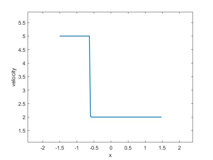
Figure 5. Density and velocity of $\delta$-shock wave for $A=1$ and $a=0.1$.

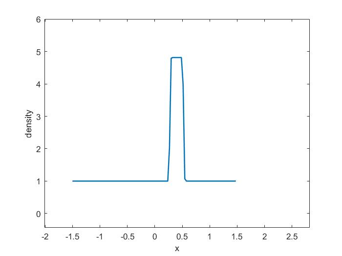
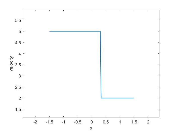
Figure 6. Density and velocity of $\delta$-shock wave for $A=0.1$ and $a=0.01.$

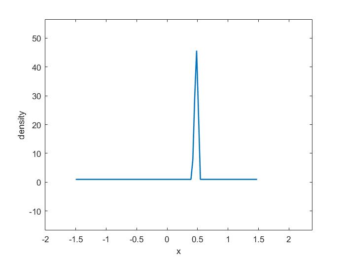
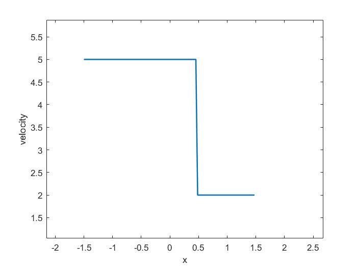
Figure 7. Density and velocity of $\delta$-shock wave for $A=0.001$ and $a=0.0001.$

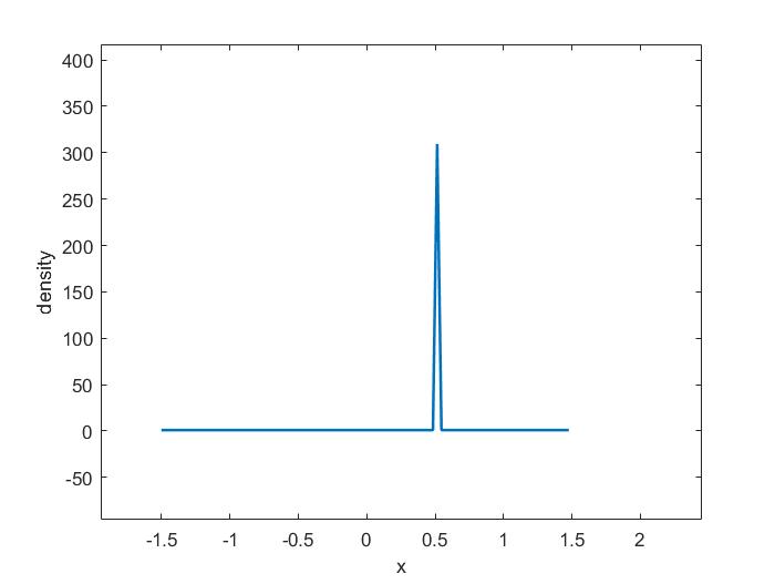
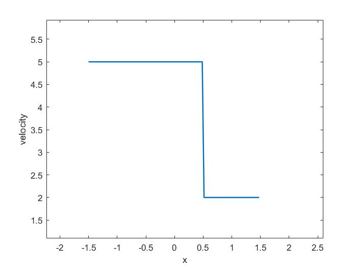
Figure 8. Density and velocity of $\delta$-shock wave for $A=0.00001$ and $a=0.000001.$

(iii) For any $\psi\in C_{0}^{\infty}(\mathbb{R}\times\mathbb{R}^{+}),$ in view of the limit of $\rho_{a}$ depending on $t,$ and (43), we have

$$\lim_{a,A\to 0}\int_{0}^{+\infty}\int_{-\infty}^{+\infty}\rho_{a}(x/t)\psi(x,t)dxdt=\lim_{a,A\to 0}\int_{0}^{+\infty}t\left(\int_{-\infty}^{+\infty}\rho_{a}(\zeta)\psi(\zeta t,t)d\zeta\right)dt$$

$$=\int_{0}^{+\infty}t\left(\rho_{l}(\upsilon_{l}-\upsilon_{r})\psi((\upsilon_{r}+\eta t)t,t)+\int_{-\infty}^{+\infty}H(\zeta-(\upsilon_{r}+\eta t))\psi(\zeta t,t)d\zeta\right)dt$$

$$=\int_{0}^{+\infty}\rho_{l}(\upsilon_{l}-\upsilon_{r})t\psi((\upsilon_{r}+\eta t)t,t)dt+\int_{0}^{+\infty}\int_{-\infty}^{+\infty}H(x-\upsilon_{r}t)\psi(x,t)dxdt$$ (44)

in which by definition (19)

$$\int_{0}^{+\infty}\rho_{l}(\upsilon_{l}-\upsilon_{r})t\psi((\upsilon_{r}+\eta t)t,t)dt=\langle p(t)\delta_{C},\psi(x,t)\rangle$$

with

$$w(t)=\rho_{l}(\upsilon_{l}-\upsilon_{r})t.$$ (45)

∎

Hence, we conclude that the Riemann solution $S+J$ converges to $\delta$-shock solution whenever $-A\left(\frac{-1}{a}\right)^{\Gamma}+\upsilon_{l}+A\left(\frac{\rho_{l}}{1-a\rho_{l}}\right)^{\Gamma}-\frac{B}{\rho_{l}^{\kappa}}<\upsilon_{r}\leqslant\upsilon_{l}-\frac{B}{\rho_{l}^{\kappa}}$ and $a,A\to 0.$ Additionally, we verify this theoretical analysis by performing numerical simulations. For this we consider $\kappa=0.5,\Gamma=2,B=1,\eta=0.2,$ and the following initial data

$$(\rho_{l,r},\upsilon_{l,r})=\begin{cases}(1,5),\qquad x<0,\\ (1,2),\qquad x>0,\end{cases}$$

in equation (32). The numerical results for different pairs of values of $a$ and $A$ are shown in figures (see, Figures 5-8). The numerical computations show that the intermediate density increases dramatically whenever $a$ and $A$ decrease. Hence, the numerical simulations verify our analysis.

3.2. Case-(ii)

Here, we analyze the Riemann solution to (6)-(7) when $\upsilon_{l}-\frac{B}{\rho_{l}^{\kappa}}<\upsilon_{r}\leqslant\upsilon_{l}$. For any $a>0$ and $A>0,$ the intermediate state $(\rho_{*},\upsilon_{*})$ is connected with $(\rho_{l},\upsilon_{l})$ by $S$ and $(\rho_{r},\upsilon_{r})$ by $J$ with speeds $\sigma_{1}$ and $\sigma_{2},$ respectively. Then, we have

$$S:\begin{cases}\sigma_{1}(t)=\upsilon_{l}+\eta t-\rho_{*}\left(\frac{A[(\rho_{*}(1-a\rho_{l}))^{\Gamma-1}+(\rho_{*}(1-a\rho_{l}))^{\Gamma-2}(\rho_{l}(1-a\rho_{*}))+\cdots+(\rho_{l}(1-a\rho_{*}))^{\Gamma-1}]}{(1-a\rho_{*})^{\Gamma}(1-a\rho_{l})^{\Gamma}}+\frac{B(\rho_{*}^{\kappa}-\rho_{l}^{\kappa})}{\rho_{*}^{\kappa}\rho_{l}^{\kappa}(\rho_{*}-\rho_{l})}\right)\vspace{0.3cm}\\ \hskip 22.76228pt\vspace{0.3cm}=\upsilon_{*}+\eta t-\rho_{l}\left(\frac{A[(\rho_{*}(1-a\rho_{l}))^{\Gamma-1}+(\rho_{*}(1-a\rho_{l}))^{\Gamma-2}(\rho_{l}(1-a\rho_{*}))+\cdots+(\rho_{l}(1-a\rho_{*}))^{\Gamma-1}]}{(1-a\rho_{*})^{\Gamma}(1-a\rho_{l})^{\Gamma}}+\frac{B(\rho_{*}^{\kappa}-\rho_{l}^{\kappa})}{\rho_{*}^{\kappa}\rho_{l}^{\kappa}(\rho_{*}-\rho_{l})}\right),\\ \frac{\upsilon_{*}-\upsilon_{l}}{\rho_{l}-\rho_{*}}=\frac{A[(\rho_{*}(1-a\rho_{l}))^{\Gamma-1}+(\rho_{*}(1-a\rho_{l}))^{\Gamma-2}(\rho_{l}(1-a\rho_{*}))+\cdots+(\rho_{l}(1-a\rho_{*}))^{\Gamma-1}]}{(1-a\rho_{*})^{\Gamma}(1-a\rho_{l})^{\Gamma}}+\frac{B(\rho_{*}^{\kappa}-\rho_{l}^{\kappa})}{\rho_{*}^{\kappa}\rho_{l}^{\kappa}(\rho_{*}-\rho_{l})},\quad\rho_{*}>\rho_{l},,\end{cases}$$ (46)

and

$$J:\begin{cases}\sigma_{2}(t)=\upsilon_{*}+\eta t=\upsilon_{r}+\eta t,\\ \upsilon_{*}=\upsilon_{r}.\end{cases}$$ (47)

From $\eqref{3.18}_{2}$ and $\eqref{3.19}_{2}$, $\rho_{*}$ satisfies

$$\upsilon_{r}=-A\left(\frac{\rho_{*}}{1-a\rho_{*}}\right)^{\Gamma}+\frac{B}{\rho_{*}^{\kappa}}+\upsilon_{l}+A\left(\frac{\rho_{l}}{1-a\rho_{l}}\right)^{\Gamma}-\frac{B}{\rho_{l}^{\kappa}}.$$ (48)

In particular, for $\Gamma=\kappa=1,$ equation (48) yields

$$\rho_{*}=\frac{-aB+\upsilon_{l}+A\left(\frac{\rho_{l}}{1-a\rho_{l}}\right)-\frac{B}{\rho_{l}}-\upsilon_{r}+\sqrt{D}}{2\left\{A+a\left(\upsilon_{l}+A\left(\frac{\rho_{l}}{1-a\rho_{l}}\right)-\frac{B}{\rho_{l}}-\upsilon_{r}\right)\right\}},$$ (49)

where

$$D=\left(aB-\upsilon_{l}-A\left(\frac{\rho_{l}}{1-a\rho_{l}}\right)+\frac{B}{\rho_{l}}+\upsilon_{r}\right)^{2}+4B\left\{A+a\left(\upsilon_{l}+A\left(\frac{\rho_{l}}{1-a\rho_{l}}\right)-\frac{B}{\rho_{l}}-\upsilon_{r}\right)\right\}.$$

Using L’Hôspital’s rule of multi variable calculus [18] in equation (49), one can obtain

$$\lim_{a,A\to 0}\rho_{*}=\frac{B}{\upsilon_{r}-\upsilon_{l}+\frac{B}{\rho_{l}}}.$$ (50)

In fact, for different pairs of values of $\Gamma$ and $\kappa,$ we verified that the $\lim_{a,A\to 0}\rho_{*}$ exists finitely (see, Table-1). We have taken $B=1$ and the initial data

$$(\rho_{l,r},\upsilon_{l,r})=\begin{cases}(1,5),\qquad x<0,\\ (1,4.5),\,\quad x>0.\end{cases}$$

$a$	$A$	$\rho_{*}$
$10^{-2}$	$10^{-1}$	1.81939694
$10^{-4}$	$10^{-3}$	3.79386025
$10^{-6}$	$10^{-5}$	3.99760412
$10^{-8}$	$10^{-7}$	3.99997600
$10^{-10}$	$10^{-9}$	3.99999976
$10^{-12}$	$10^{-11}$	4.00000000
$10^{-14}$	$10^{-13}$	4.00000000
2.2204$\times$ $10^{-16}$	2.2204$\times$ $10^{-16}$	4.00000000

Table 1. The intermediate densities for values $a$ and $A$ with $\Gamma$=2 and $\kappa=0.5.$

3.3. Limit of Riemann solutions when ($\rho_{r}$, $\upsilon_{r}$) lies in Region-III

We study the limit $a,A\to 0$ of the Riemann solution to (6) with (7) in the case $\upsilon_{l}<\upsilon_{r}$. For any $a>0$ and $A>0$, the intermediate state $(\rho_{*},\upsilon_{*})$ is connected with $(\rho_{l},\upsilon_{l})$ by $R$ and $(\rho_{r},\upsilon_{r})$ by $J$, respectively. Then, we have

$$R:\begin{cases}\zeta=\lambda_{1}=\upsilon+\eta t-\frac{\Gamma A\rho^{\Gamma}}{(1-a\rho)^{\Gamma+1}}-\frac{\kappa B}{\rho^{\kappa}},\qquad\rho_{*}<\rho<\rho_{l},\vspace{0.3cm}\\ \frac{\upsilon-\upsilon_{l}}{\rho_{l}-\rho}=\frac{A[(\rho(1-a\rho_{l}))^{\Gamma-1}+(\rho(1-a\rho_{l}))^{\Gamma-2}(\rho_{l}(1-a\rho))+\cdots+(\rho_{l}(1-a\rho))^{\Gamma-1}]}{(1-a\rho)^{\Gamma}(1-a\rho_{l})^{\Gamma}}+\frac{B(\rho^{\kappa}-\rho_{l}^{\kappa})}{\rho^{\kappa}\rho_{l}^{\kappa}(\rho-\rho_{l})},\end{cases}$$ (51)

and

$$J:\begin{cases}\sigma_{2}(t)=\upsilon_{*}+\eta t=\upsilon_{r}+\eta t,\\ \upsilon_{*}=\upsilon_{r}.\end{cases}$$ (52)

From $\eqref{4.1}_{2}$ and $\eqref{4.2}_{2}$, $\rho_{*}$ satisfies

$$\upsilon_{r}=-A\left(\frac{\rho_{*}}{1-a\rho_{*}}\right)^{\Gamma}+\frac{B}{\rho_{*}^{\kappa}}+\upsilon_{l}+A\left(\frac{\rho_{l}}{1-a\rho_{l}}\right)^{\Gamma}-\frac{B}{\rho_{l}^{\kappa}}.$$ (53)

Taking $\lim_{a,A\to 0}$ in (53), with the consideration that $\lim_{a,A\to 0}\rho_{*}=0,$ one can obtain $\upsilon_{r}=+\infty,$ which is absurd. Hence, there is no vacuum in the Riemann solution of the system (6)-(7).

4. Behavior of Riemann solutions as pressure falls to zero i.e., $a,A,B\to 0.$

On the basis of relations between $\upsilon_{l}$ and $\upsilon_{r},$ we divide this discussion into the following three cases:

4.1. Case-(i): $\upsilon_{l}$ $>$ $\upsilon_{r}$

In this case, ($\rho_{r}$, $\upsilon_{r}$) lies in region-I or region-II. If the right state ($\rho_{r}$, $\upsilon_{r}$) lies in the region-I, then the Riemann solution is given by (22) with (23)-(27). It is easy to see that when $a,A,B\to 0,$ for $\rho_{r}\neq\rho_{l},$

$$\upsilon_{\delta}=\frac{\upsilon_{l}\sqrt{\rho_{l}}+\upsilon_{r}\sqrt{\rho_{r}}}{\sqrt{\rho_{l}}+\sqrt{\rho_{r}}},\quad\sigma(t)=\upsilon_{\delta}+\eta t,\quad x(t)=\upsilon_{\delta}t+\frac{1}{2}\eta t^{2},\quad w(t)=\sqrt{\rho_{l}\rho_{r}}(\upsilon_{l}-\upsilon_{r})t.$$ (54)

For $\rho_{r}=\rho_{l},$

$$\upsilon_{\delta}=\frac{\upsilon_{l}+\upsilon_{r}}{2},\quad\sigma(t)=\upsilon_{\delta}+\eta t,\quad x(t)=\upsilon_{\delta}t+\frac{1}{2}\eta t^{2},\quad w(t)=\rho_{l}(\upsilon_{l}-\upsilon_{r})t.$$ (55)

If the right state ($\rho_{r}$, $\upsilon_{r}$) lies in region-II, then the Riemann solution is given by $S+J.$ A similar calculation, as we have done in case (i) of section-$3,$ shows that the solution $S+J$ converges to delta shock solution of the transport equations with the same friction term as $a,A,B\to 0.$

4.2. Case-(ii): $\upsilon_{l}$ $=$ $\upsilon_{r}$

For this case, the Riemann solution is given by the contact discontinuity $J$.

4.3. Case-(iii): $\upsilon_{l}$ $<$ $\upsilon_{r}$

For any $a>0,$ $A>0,$ and $B>0$, the intermediate state $(\rho_{*},\upsilon_{*})$ is connected with $(\rho_{l},\upsilon_{l})$ by $R$ and $(\rho_{r},\upsilon_{r})$ by $J$, then we have

$$R:\begin{cases}\zeta=\lambda_{1}=\upsilon+\eta t-\frac{\Gamma A\rho^{\Gamma}}{(1-a\rho)^{\Gamma+1}}-\frac{\kappa B}{\rho^{\kappa}},\qquad\rho_{*}<\rho<\rho_{l},\vspace{0.3cm}\\ \frac{\upsilon-\upsilon_{l}}{\rho_{l}-\rho}=\frac{A[(\rho(1-a\rho_{l}))^{\Gamma-1}+(\rho(1-a\rho_{l}))^{\Gamma-2}(\rho_{l}(1-a\rho))+\cdots+(\rho_{l}(1-a\rho))^{\Gamma-1}]}{(1-a\rho)^{\Gamma}(1-a\rho_{l})^{\Gamma}}+\frac{B(\rho^{\kappa}-\rho_{l}^{\kappa})}{\rho^{\kappa}\rho_{l}^{\kappa}(\rho-\rho_{l})},\end{cases}$$ (56)

and

$$J:\begin{cases}\sigma_{2}(t)=\upsilon_{*}+\eta t=\upsilon_{r}+\eta t,\\ \upsilon_{*}=\upsilon_{r}.\end{cases}$$ (57)

From $\eqref{4.1}_{2}$ and $\eqref{4.2}_{2}$, $\rho_{*}$ satisfies

$$\upsilon_{r}=-A\left(\frac{\rho_{*}}{1-a\rho_{*}}\right)^{\Gamma}+\frac{B}{\rho_{*}^{\kappa}}+\upsilon_{l}+A\left(\frac{\rho_{l}}{1-a\rho_{l}}\right)^{\Gamma}-\frac{B}{\rho_{l}^{\kappa}}.$$ (58)

Taking $\lim_{a,A,B\to 0}$ in (58), with the consideration that $\lim_{a,A\to 0}\rho_{*}\neq 0,$ one can obtain $\upsilon_{r}=\upsilon_{l},$ which contradicts with $\upsilon_{r}>\upsilon_{l}.$ Hence, the vacuum state occurs in the Riemann solution of the system (6)-(7). Furthermore, the Riemann solution for this case is express as

$$\lim_{a,A,B\to 0}(\rho,\upsilon)(x,t)=\begin{cases}(\rho_{l},\upsilon_{l}),\hskip 28.45274ptx<\upsilon_{l}t+\frac{1}{2}\eta t^{2},\\ \text{vacuum},\hskip 19.91684pt\upsilon_{l}t+\frac{1}{2}\eta t^{2}<x<\upsilon_{r}t+\frac{1}{2}\eta t^{2},\\ (\rho_{r},\upsilon_{r}),\hskip 27.03003ptx>\upsilon_{r}t+\frac{1}{2}\eta t^{2}.\end{cases}$$ (59)

Hence, the Riemann solutions of our system coincide with the corresponding Riemann solutions of the transport equations with the same source term as pressure falls to zero.

5. Solutions of the original Riemann problem (3)-(5)

Here, we turn back our attention to the original Riemann problem (3)-(5). Before going on to the original Riemann problem it is noted that we have taken $u_{l}=\upsilon_{l}$ and $u_{r}=\upsilon_{r}$ in our aforementioned work(only for convenience). Now, based on some special conditions on the initial data (5), we divide this discussion into three parts:
(i) If $(\rho_{r},u_{r})$ lies in region-II, i.e., $-A\left(\frac{-1}{a}\right)^{\Gamma}+u_{l}+A\left(\frac{\rho_{l}}{1-a\rho_{l}}\right)^{\Gamma}-\frac{B}{\rho_{l}^{\kappa}}<u_{r}\leqslant u_{l},$ then the Riemann solution of (3)-(5) is represented as (see Figure 9(A))

$$(\rho,u)(x,t)=\begin{cases}(\rho_{l},u_{l}+\eta t),\qquad x<x_{1}(t),\\ (\rho_{*},u_{*}+\eta t),\qquad x_{1}(t)<x<x_{2}(t),\\ (\rho_{r},u_{r}+\eta t),\qquad x_{2}(t)<x,\end{cases}$$ (60)

where

$$x_{1}(t)= u_{l}t-\rho_{*}\left(\frac{B(\rho_{*}^{\kappa}-\rho_{l}^{\kappa})}{\rho_{*}^{\kappa}\rho_{l}^{\kappa}(\rho_{*}-\rho_{l})}\right)t+\frac{1}{2}\eta t^{2}$$

$$-\rho_{*}\left(\frac{A[(\rho_{*}(1-a\rho_{l}))^{\Gamma-1}+(\rho_{*}(1-a\rho_{l}))^{\Gamma-2}(\rho_{l}(1-a\rho_{*}))+\cdots+(\rho_{l}(1-a\rho_{*}))^{\Gamma-1}]}{(1-a\rho_{*})^{\Gamma}(1-a\rho_{l})^{\Gamma}}\right)t,$$

represents the equation of shock wave curve and $x_{2}(t)=u_{r}t+\frac{1}{2}\eta t^{2}$ represents the equation of contact discontinuity curve. Also, the intermediate state $(\rho_{*},u_{*}+\eta t)$ between the shock wave($S$) and contact discontinuity($J$) can be obtained directly from the following expressions

$$u_{l}+A\left(\frac{\rho_{l}}{1-a\rho_{l}}\right)^{\Gamma}-\frac{B}{\rho_{l}^{\kappa}}=u_{*}+A\left(\frac{\rho_{*}}{1-a\rho_{*}}\right)^{\Gamma}-\frac{B}{\rho_{*}^{\kappa}},\qquad u_{*}=u_{r}.$$ (61)

(ii) If $(\rho_{r},u_{r})$ lies in region-III, i.e., $u_{l}<u_{r},$ then the solution of the Riemann problem (3)-(5) is expressed as (see Figure 9(B))

$$(\rho,u)(x,t)=\begin{cases}(\rho_{l},u_{l}+\eta t),\qquad x<x_{1}^{l}(t),\\ (\rho_{2},u_{2}+\eta t),\qquad x_{1}^{l}(t)<x<x_{1}^{*}(t),\\ (\rho_{*},u_{*}+\eta t),\qquad x_{1}^{*}(t)<x<x_{2}(t),\\ (\rho_{r},u_{r}+\eta t),\qquad x_{2}(t)<x,\end{cases}$$ (62)

where

$$x_{1}^{l}(t)=u_{l}+\eta t-\frac{\Gamma A\rho_{l}^{\Gamma}}{(1-a\rho_{l})^{\Gamma+1}}-\frac{\kappa B}{\rho_{l}^{\kappa}},$$

$$x_{1}^{*}(t)=u_{*}+\eta t-\frac{\Gamma A\rho_{*}^{\Gamma}}{(1-a\rho_{*})^{\Gamma+1}}-\frac{\kappa B}{\rho_{*}^{\kappa}},$$

$$x_{2}(t)=u_{r}+\eta t,$$

represent the equations of left most edge of rarefaction wave curve, right most edge of rarefaction wave curve and contact discontinuity curve, respectively. Also, the intermediate state $(\rho_{*},u_{*}+\eta t)$ between the rarefaction wave($R$) and contact discontinuity($J$) can be obtained directly from the following expressions

$$u_{l}+A\left(\frac{\rho_{l}}{1-a\rho_{l}}\right)^{\Gamma}-\frac{B}{\rho_{l}^{\kappa}}=u_{*}+A\left(\frac{\rho_{*}}{1-a\rho_{*}}\right)^{\Gamma}-\frac{B}{\rho_{*}^{\kappa}},\qquad u_{*}=u_{r}.$$ (63)

(a) If $(\rho_{r},u_{r})$ lies in region-II.

(b) If $(\rho_{r},u_{r})$ lies in region-III.

Figure 9. Riemann solutions of (3)-(5) in $(x,t)$-plane when $\eta>0.$

(iii) If $(\rho_{r},u_{r})$ lies in region-I, i.e., $u_{r}\leqslant-A\left(\frac{-1}{a}\right)^{\Gamma}+u_{l}+A\left(\frac{\rho_{l}}{1-a\rho_{l}}\right)^{\Gamma}-\frac{B}{\rho_{l}^{\kappa}},$ then the Riemann solution of (3)-(5) is given by a single delta shock wave curve(see, Figure 10). In this case, the Riemann solution is defined as follow

Definition 5.1.

Let ($\rho,u$) be a pair of distributions where $\rho(x,t)=\hat{\rho}(x,t)+\omega(x,t)\delta(\gamma)$ and $\hat{\rho},u$ $\in$ $L^{\infty}(\mathbb{R}\times\mathbb{R}^{+}).$ Then ($\rho,u$) is called the delta shock solution of the Riemann problem (3)-(5) if the followings hold [21]

$$\begin{cases}\langle\rho,\psi_{t}\rangle+\langle\rho u,\psi_{x}\rangle=0,\\ \langle\rho\left(u+A\left(\frac{\rho}{1-a\rho}\right)^{\Gamma}-\frac{B}{\rho^{\kappa}}\right),\psi_{t}\rangle+\langle\rho u\left(u+A\left(\frac{\rho}{1-a\rho}\right)^{\Gamma}-\frac{B}{\rho^{\kappa}}\right),\psi_{x}\rangle=-\langle\eta\rho,\psi\rangle,\end{cases}$$ (64)

for all the test functions $\psi\in C_{0}^{\infty}(\mathbb{R}\times\mathbb{R}^{+}).$ Here, we take

$$\langle\rho u\left(u+A\left(\frac{\rho}{1-a\rho}\right)^{\Gamma}-\frac{B}{\rho^{\kappa}}\right),\psi\rangle=\int_{0}^{+\infty}\int_{-\infty}^{+\infty}\hat{\rho}u\left(u+A\left(\frac{\hat{\rho}}{1-a\hat{\rho}}\right)^{\Gamma}-\frac{B}{\hat{\rho}^{\kappa}}\right)\psi dxdt+\langle\omega u_{\delta}^{2}(t)\delta_{C},\psi\rangle,$$ (65)

where $u_{\delta}(t)$ is the value of $u$ on the delta shock wave curve.

(a) $\eta>0$.

(b) $\eta<0$.

Figure 10. Riemann solutions of (3)-(5) in $(x,t)$-plane when $(\rho_{r},u_{r})\in\text{I}$.

Thus, for $u_{r}\leqslant-A\left(\frac{-1}{a}\right)^{\Gamma}+u_{l}+A\left(\frac{\rho_{l}}{1-a\rho_{l}}\right)^{\Gamma}-\frac{B}{\rho_{l}^{\kappa}},$ we seek for a piece-wise smooth solution of the Riemann problem(3)-(5) in the following form

$$(\rho,u)(x,t)=\begin{cases}(\rho_{l},u_{l}+\eta t),\qquad\qquad\,\qquad\quad x<x(t),\\ (\omega(t)\delta(x-x(t)),u_{\delta}(t)),\,\,\qquad x=x(t),\\ (\rho_{r},u_{r}+\eta t),\qquad\qquad\quad\qquad x>x(t).\end{cases}$$ (66)

           It is noted that $u_{\delta}(t)-\eta t$ is assumed to be a constant. Similarly, as we have done, in section-2, the delta shock solution (66) should satisfy the following generalized Rankine-Hugoniot jump conditions

$$\begin{cases}\frac{dx(t)}{dt}=\sigma(t)=u_{\delta}(t),\\ \frac{dw(t)}{dt}=-[\rho]\sigma(t)+[\rho u],\\ \frac{d(w(t)u_{\delta}(t))}{dt}=-\left[\rho\left(u+A\left(\frac{\rho}{1-a\rho}\right)^{\Gamma}-\frac{B}{\rho^{\kappa}}\right)\right]\sigma(t)+\left[\rho u\left(u+A\left(\frac{\rho}{1-a\rho}\right)^{\Gamma}-\frac{B}{\rho^{\kappa}}\right)\right]+\beta\omega(t),\end{cases}$$ (67)

where

$$\begin{cases}[\rho u]=\rho_{l}(u_{l}+\eta t)-\rho_{r}(u_{r}+\eta t),\\ \left[\rho\left(u+A\left(\frac{\rho}{1-a\rho}\right)^{\Gamma}-\frac{B}{\rho^{\kappa}}\right)\right]=\rho_{l}\left(u_{l}+\eta t+A\left(\frac{\rho_{l}}{1-a\rho_{l}}\right)^{\Gamma}-\frac{B}{\rho_{l}^{\kappa}}\right)-\rho_{r}\left(u_{r}+\eta t+A\left(\frac{\rho_{r}}{1-a\rho_{r}}\right)^{\Gamma}-\frac{B}{\rho_{r}^{\kappa}}\right).\end{cases}$$

In order to ensure the uniqueness, the measure solution (66) should satisfy the followings entropy condition

$$u_{r}+\eta t-\frac{\Gamma A\rho_{r}^{\Gamma}}{(1-a\rho_{r})^{\Gamma+1}}-\frac{\kappa B}{\rho_{r}^{\kappa}}<u_{r}+\eta t\leqslant u_{\delta}(t)\leqslant u_{l}+\eta t-\frac{\Gamma A\rho_{l}^{\Gamma}}{(1-a\rho_{l})^{\Gamma+1}}-\frac{\kappa B}{\rho_{l}^{\kappa}}<u_{l}+\eta t.$$

           To define the Riemann solution of (3)-(5), we propose the following theorem:

Theorem 5.2.

For the case $u_{r}\leqslant-A\left(\frac{-1}{a}\right)^{\Gamma}+u_{l}+A\left(\frac{\rho_{l}}{1-a\rho_{l}}\right)^{\Gamma}-\frac{B}{\rho_{l}^{\kappa}},$ the Riemann solution of (3)-(5) should have the following $\delta$-shock solution

$$(\rho,u)(x,t)=\begin{cases}(\rho_{l},u_{l}+\eta t),\qquad\qquad\,\qquad\quad x<x(t),\\ (\omega(t)\delta(x-x(t)),u_{\delta}(t)),\,\,\qquad x=x(t),\\ (\rho_{r},u_{r}+\eta t),\qquad\qquad\quad\qquad x>x(t),\end{cases}$$ (68)

in which

$$\begin{cases}\sigma(t)=u_{\delta}(t)=\upsilon_{\delta}+\eta t,\\ \upsilon_{\delta}=\frac{2(\rho_{l}u_{l}-\rho_{r}u_{r})+D_{1}-D_{2}}{2(\rho_{l}-\rho_{r})},\\ x(t)=\upsilon_{\delta}t+\frac{1}{2}\eta t^{2},\\ w(t)=\frac{-D_{1}+D_{2}}{2}t,\end{cases}\qquad\text{if}\,\,\rho_{l}\neq\rho_{r},$$ (69)

where

$$D_{1}=A\left(\frac{\rho_{l}^{\Gamma+1}}{(1-a\rho_{l})^{\Gamma}}\right)-\frac{B}{\rho_{l}^{\kappa-1}}-A\left(\frac{\rho_{r}^{\Gamma+1}}{(1-a\rho_{r})^{\Gamma}}\right)+\frac{B}{\rho_{r}^{\kappa-1}},$$ (70)

$$D_{2}=\sqrt{4\rho_{l}\rho_{r}(u_{l}-u_{r})(u_{l}-u_{r}+D_{3})+D_{1}^{2}},\hskip 72.2698pt$$ (71)

$$D_{3}=A\left(\frac{\rho_{l}}{1-a\rho_{l}}\right)^{\Gamma}-\frac{B}{\rho_{l}^{\kappa}}-A\left(\frac{\rho_{r}}{1-a\rho_{r}}\right)^{\Gamma}+\frac{B}{\rho_{r}^{\kappa}},\hskip 41.25641pt$$ (72)

and

$$\begin{cases}\sigma(t)=u_{\delta}(t)=\upsilon_{\delta}+\eta t,\\ \upsilon_{\delta}=\frac{u_{r}+u_{l}}{2}+\frac{A}{2}\left(\frac{\rho_{l}}{1-a\rho_{l}}\right)^{\Gamma}-\frac{B}{2\rho_{l}^{\kappa}},\\ x(t)=\upsilon_{\delta}t+\frac{1}{2}\eta t^{2},\\ w(t)=\rho_{l}(u_{l}-u_{r})t,\end{cases}\text{if}\,\,\rho_{l}=\rho_{r}.$$ (73)

Proof.

As $u_{\delta}(t)-\eta t$ is constant, therefore, $\eqref{9.8}$ implies that

$$(u_{\delta}(t)-\eta t)^{2}(\rho_{l}-\rho_{r})-(u_{\delta}(t)-\eta t)(2\rho_{l}u_{l}+\rho_{l}P_{l}-2\rho_{r}u_{r}-\rho_{r}P_{r})+\rho_{l}u_{l}(u_{l}+P_{l}-\rho_{r}u_{r}(u_{r}+P_{r}))=0,$$ (74)

in which $P_{l}=A\left(\frac{\rho_{l}}{1-a\rho_{l}}\right)^{\Gamma}-\frac{B}{\rho_{l}^{\kappa}}$ and $P_{r}=A\left(\frac{\rho_{r}}{1-a\rho_{r}}\right)^{\Gamma}-\frac{B}{\rho_{r}^{\kappa}}.$ Also, (74) gives that

$$u_{\delta}(t)=\begin{cases}\frac{2(\rho_{l}u_{l}-\rho_{r}u_{r})+D_{1}-D_{2}}{2(\rho_{l}-\rho_{r})}+\eta t,\qquad\quad\,\qquad\text{if}\quad\rho_{l}\neq\rho_{r},\\ \frac{u_{r}+u_{l}}{2}+\frac{A}{2}\left(\frac{\rho_{l}}{1-a\rho_{l}}\right)^{\Gamma}-\frac{B}{2\rho_{l}^{\kappa}}+\eta t,\qquad\text{if}\quad\rho_{l}=\rho_{r}.\end{cases}$$ (75)

Hence, $u_{\delta}(t)=\upsilon_{\delta}+\eta t.$ Now, we have to prove that measure solution (68)-(73) satisfy the system (3)-(4) in the distributional sense, i.e.,

$$\begin{cases}I_{1}=\langle\rho,\psi_{t}\rangle+\langle\rho u,\psi_{x}\rangle=0,\\ I_{2}=\langle\rho\left(u+A\left(\frac{\rho}{1-a\rho}\right)^{\Gamma}-\frac{B}{\rho^{\kappa}}\right),\psi_{t}\rangle+\langle\rho u\left(u+A\left(\frac{\rho}{1-a\rho}\right)^{\Gamma}-\frac{B}{\rho^{\kappa}}\right),\psi_{x}\rangle=-\langle\eta\rho,\psi\rangle,\end{cases}$$ (76)

for all the test functions $\psi\in C_{0}^{\infty}(\mathbb{R}\times\mathbb{R}^{+}).$
           It is noted that the delta shock wave curve, $x(t),$ is strictly monotonically increasing for $\eta>0$. Therefore, inverse of $x(t)$ exists globally, which is defined as

$$t(x)=\sqrt{\frac{\upsilon_{\delta}^{2}}{\eta^{2}}+\frac{2x}{\eta}}-\frac{\upsilon_{\delta}}{\eta}.$$

When $\eta<0,$ the delta shock wave curve, $x(t),$ has a critical point, namely $\left(\frac{-\upsilon_{\delta}^{2}}{\eta},\frac{-\upsilon_{\delta}}{\eta}\right).$ Thus, the inverse of $x(t)$ is given as

$$t(x)=\begin{cases}-\sqrt{\frac{\upsilon_{\delta}^{2}}{\eta^{2}}+\frac{2x}{\eta}}-\frac{\upsilon_{\delta}}{\eta},\qquad t\leq-\frac{\upsilon_{\delta}}{\eta},\\ \sqrt{\frac{\upsilon_{\delta}^{2}}{\eta^{2}}+\frac{2x}{\eta}}-\frac{\upsilon_{\delta}}{\eta},\,\qquad\,\,\,t>-\frac{\upsilon_{\delta}}{\eta},\end{cases}$$ (77)

For simplicity, we consider that $\eta>0.$ The other case can be treated in a similar manner. With this consideration, we have

$$\frac{d(\psi(x(t),t))}{dt}=\psi_{t}(x,t)+\frac{dx}{dt}\psi_{x}(x,t)=\psi_{t}(x,t)+(\upsilon_{\delta}+\eta t)\psi_{x}(x,t)=\psi_{t}(x,t)+u_{\delta}(t)\psi_{x}(x,t).$$ (78)

Also, we have

$$I_{2}=\int_{0}^{+\infty}\int_{-\infty}^{+\infty}\left(\rho\left(u+A\left(\frac{\rho}{1-a\rho}\right)^{\Gamma}-\frac{B}{\rho^{\kappa}}\right)\psi_{t}+\rho u\left(u+A\left(\frac{\rho}{1-a\rho}\right)^{\Gamma}-\frac{B}{\rho^{\kappa}}\right)\psi_{x}\right)dxdt$$

$$=\int_{0}^{+\infty}\int_{-\infty}^{x(t)}\left(\rho_{l}\left(u_{l}+\eta t+P_{l}\right)\psi_{t}+\rho_{l}(u_{l}+\eta t)\left(u_{l}+\eta t+P_{l}\right)\psi_{x}\right)dxdt$$

$${}+\int_{0}^{+\infty}\int_{x(t)}^{+\infty}\left(\rho_{r}\left(u_{r}+\eta t+P_{r}\right)\psi_{t}+\rho_{r}(u_{r}+\eta t)\left(u_{r}+\eta t+P_{r}\right)\psi_{x}\right)dxdt$$

$${}{}+\int_{0}^{+\infty}\omega(t)(\upsilon_{\delta}+\eta t)\left(\psi_{t}(x(t),t)+(\upsilon_{\delta}+\eta t)\psi_{x}(x(t),t)\right)dt.$$

By exchanging the ordering of integral and using integration by parts, we have

$$I_{2}=\int_{0}^{+\infty}\int_{t(x)}^{+\infty}\rho_{l}\left(u_{l}+\eta t+P_{l}\right)\psi_{t}dtdx+\int_{0}^{+\infty}\int_{-\infty}^{x(t)}\rho_{l}(u_{l}+\eta t)\left(u_{l}+\eta t+P_{l}\right)\psi_{x}dxdt$$

$${}+\int_{0}^{+\infty}\int_{0}^{t(x)}\rho_{r}\left(u_{r}+\eta t+P_{r}\right)\psi_{t}dtdx+\int_{0}^{+\infty}\int_{x(t)}^{+\infty}\rho_{r}(u_{r}+\eta t)\left(u_{r}+\eta t+P_{r}\right)\psi_{x}dxdt$$

$${}{}+\int_{0}^{+\infty}\omega(t)(\upsilon_{\delta}+\eta t)d\psi(x(t),t)$$

$$=\int_{0}^{+\infty}(\rho_{r}(u_{r}+\eta t(x)+P_{r})-\rho_{l}(u_{l}+\eta t(x)+P_{l}))\psi(x,t(x))dx$$

$$+\int_{0}^{+\infty}(\rho_{l}(u_{l}+\eta t)(u_{l}+\eta t+P_{l})-\rho_{r}(u_{r}+\eta t)(u_{r}+\eta t+P_{r}))\psi(x(t),t)dt$$

$$-\int_{0}^{+\infty}\int_{t(x)}^{+\infty}\eta\rho_{l}\psi dtdx-\int_{0}^{+\infty}\int_{0}^{t(x)}\eta\rho_{r}\psi dtdx-\int_{0}^{+\infty}\left(\frac{-D_{1}+D_{2}}{2}\right)(\upsilon_{\delta}+2\eta t)\psi(x(t),t)dt,$$

$$=\int_{0}^{+\infty}E(t)\psi(x(t),t)dt-\eta\left(\int_{0}^{+\infty}\int_{-\infty}^{x(t)}\rho_{l}\psi dxdt+\int_{0}^{+\infty}\int_{x(t)}^{+\infty}\rho_{r}\psi dxdt\right),$$ (79)

where

$$E(t)= \left(\rho_{r}\left(u_{r}+\eta t+P_{r}\right)-\rho_{l}\left(u_{l}+\eta t+P_{l}\right)\right)\left(\upsilon_{\delta}+\eta t\right)-\rho_{r}(u_{r}+\eta t)\left(u_{r}+\eta t+P_{r}\right)$$

$$+\rho_{l}(u_{l}+\eta t)\left(u_{l}+\eta t+P_{l}\right)-\left(\frac{-D_{1}+D_{2}}{2}\right)(\upsilon_{\delta}+2\eta t).$$

On simplification, one can have

$$E(t)=-\eta\left(\frac{-D_{1}+D_{2}}{2}\right)t=-\eta\omega(t).$$ (80)

Thus, (5) and (80) together imply that the second equation of (76) holds. In a similar way, $\eqref{9.12}_{1}$ can be proved.

∎

Remark 5.3.

The limiting behavior of the Riemann solutions to (3)-(5) can be analyzed by following the same approach as we have applied in sections $3$ and $4$.

6. Conclusion and Discussion

In this work, we have obtained the Riemann solutions of Aw-Rascle model with friction for a more realistic version of extended Chaplygin gas. In section-$2,$ we established that for $\upsilon_{r}\leqslant-A\left(\frac{-1}{a}\right)^{\Gamma}+\upsilon_{l}+A\left(\frac{\rho_{l}}{1-a\rho_{l}}\right)^{\Gamma}-\frac{B}{\rho_{l}^{\kappa}},$ delta shock is formed in the Riemann solution. Additionally, in section-$3,$ we found that the Riemann solution $S+J$ converges to $\delta$-shock solution whenever $-A\left(\frac{-1}{a}\right)^{\Gamma}+\upsilon_{l}+A\left(\frac{\rho_{l}}{1-a\rho_{l}}\right)^{\Gamma}-\frac{B}{\rho_{l}^{\kappa}}<\upsilon_{r}\leqslant\upsilon_{l}-\frac{B}{\rho_{l}^{\kappa}}$ and $a,A\to 0.$ Moreover, in section-$4,$ we obtained that our Riemann solutions converge to the corresponding Riemann solutions of the transport equations with the same source term as $a,A,B\to 0$. Furthermore, in section-5, the Riemann solutions of the original Riemann problem (3)-(5) are constructed explicitly. These results imply the conditions on the initial data and pressure under which delta shock is formed in the Riemann solutions. Hence, we have found the conditions during which jam occurs in traffic flow. In theorem $3.5,$ we have calculated that how much mass is accumulated in time $t$ whenever $S+J$ converges to $\delta$-shock solution. Physically, it explains about the concentration of traffic when jam occurs in traffic flow. The Coulomb like friction term in $(3)$ describes the granular flow behavior. In traffic flow model, it explains the traffic flow on an inclined road. Further, we established that due to the presence of Coulomb like friction term, the characteristic curves bend into the parabolic shape implying thereby that the delta shock wave discontinuity is also parabolic curved. Hence, the Aw-Rascle model with friction elucidates the dynamics and formation of traffic jam in traffic flow on an inclined road. We have constructed the Riemann solutions of $(3)$ by considering more generalized value of the pressure $p.$ With the use of these Riemann solutions, one can directly obtain the Riemann solutions of $(3)$ with various equation of state (according to the requirement) by inserting the particular values of $A,$ $B,$ $\Gamma,$ $a,$ and $\kappa$ in these solutions. Further, by considering friction term $\eta=0,$ one can get the Riemann solutions of the corresponding homogeneous Aw-Rascle model. We have precisely investigated that our results for the specific values of $A,$ $B,$ $\Gamma,$ $a,$ $\kappa,$ and $\eta$ coincide with the existing one; e.g., by taking $\Gamma=\kappa=1$ and $a=\eta=0$ in the Riemann solutions of (3) with (4), we directly obtain the Riemann solutions of traffic flow model for modified Chaplygin gas [8]. Furthermore, for $A=\eta=0$ and $\kappa=1$, we get the Riemann solution of Chaplygin Aw-Rascle model [22], and for $A=0$ and $\kappa=1$ in $(4)$ our Riemann solutions coincide with the Riemann solutions of Aw-Rascle model with friction for Modified Chaplygin gas [41]. Also, the approach used in this work can be applied to the non-symmetric Keyfitz-Kranzer type system [5, 7] for the Chaplygin pressure and Coulomb like friction.

Acknowledgements. The supports provided by UGC, India (Ref. No.:201610063559) and NBHM, India (Ref. No.: NBHM(RP)/R&D II/7857) are gratefully acknowledged by Priyanka and M. Zafar, respectively.

Data Availability. Data sharing is not applicable to this article as no new data were created or analyzed in this study.

References

• [1] A. Aw and M. Rascle. Resurrection of ”second order” models of traffic flow. SIAM Journal of Applied Mathematics, 60(3):916–938, 2000.
• [2] R. Barthwal and T. Raja Sekhar. Simple waves for two-dimensional magnetohydrodynamics with extended Chaplygin gas. Indian Journal of Pure and Applied Mathematics, 53(2):542–549, 2022.
• [3] Y. Brenier and E. Grenier. Sticky particles and scalar conservation laws. SIAM Journal of Numerical Analysis, 35(6):2317–2328, 1998.
• [4] S. Chaplygin. On gas jets, Scientific Memoirs, Moscow University Mathematics Physics 21 (1904) pp. 1-127. Translated by M. Slud, Brown University, 1944.
• [5] H. Cheng. Delta shock waves for a linearly degenerate hyperbolic system of conservation laws of Keyfitz-Kranzer type. Advances in Mathematical Physics, 2013.
• [6] H. Cheng, W. Liu, and H. Yang. Two-dimensional Riemann problems for zero-pressure gas dynamics with three constant states. Journal of Mathematical Analysis and Applications, 343(1):127–140, 2008.
• [7] H. Cheng and H. Yang. On a nonsymmetric Keyfitz-Kranzer system of conservation laws with generalized and modified Chaplygin gas pressure law. Advances in Mathematical Physics, 2013.
• [8] H. Cheng and H. Yang. Approaching Chaplygin pressure limit of solutions to the Aw–Rascle model. Journal of Mathematical Analysis and Applications, 416(2):839–854, 2014.
• [9] C. Daganzo. Requiem for second-order fluid approximations of traffic flow. Transportation Research Part B: Methodological, 29(4):277–286, 1995.
• [10] V. G. Danilov and V. M. Shelkovich. Dynamics of propagation and interaction of $\delta$-shock waves in conservation law systems. Journal of Differential Equations, 211(2):333–381, 2005.
• [11] W. E., Yu. G. Rykov, and Ya. G. Sinai. Generalized variational principles, global weak solutions and behavior with random initial data for systems of conservation laws arising in adhesion particle dynamics. Communications in Mathematical Physics, 177(2):349–380, 1996.
• [12] G. Faccanoni and A. Mangeney. Exact solution for granular flows. International Journal for Numerical and Analytical Methods in Geomechanics, 37(10):1408–1433, 2013.
• [13] S. Fan and Y. Zhang. Wave interactions and stability of Riemann solutions to the Aw-Rascle model with friction for modified Chaplygin gas. Bulletin of the Brazilian Mathematical Society, New Series, pages 1–21, 2022.
• [14] S. Fan and Y. Zhang. Riemann problem and wave interactions for an inhomogeneous Aw-Rascle traffic flow model with extended Chaplygin gas. International Journal of Non-Linear Mechanics, 152:104384, 2023.
• [15] F. Huang and Z. Wang. Well-posedness for pressureless flow. Communications in Mathematical Physics, 222(1):117–146, 2001.
• [16] W. Jiang, T. Chen, T. Li, and Z. Wang. The Riemann problem with delta initial data for the non-isentropic improved Aw-Rascle-Zhang model. Acta Mathematica Scientia, 43(1):237–258, 2023.
• [17] K.T. Joseph. A Riemann problem whose viscosity solutions contain $\delta$-measures. Asymptotic Analysis, 7(2):105–120, 1993.
• [18] G. R. Lawlor. A L’hospital’s rule for multivariable functions. arXiv preprint arXiv:1209.0363, 2012.
• [19] J. Li and H. Yang. Delta-shocks as limits of vanishing viscosity for multidimensional zero-pressure gas dynamics. Quarterly of Applied mathematics, 59(2):315–342, 2001.
• [20] J. Li, T. Zhang, and S. Yang. The two-dimensional Riemann problem in gas dynamics, volume 98. CRC Press, 1998.
• [21] S. Li. Riemann solutions of the anti-Chaplygin pressure Aw–Rascle model with friction. Journal of Mathematical Physics, 63(12), 2022.
• [22] L. Pan and X. Han. The Aw–Rascle traffic model with Chaplygin pressure. Journal of Mathematical Analysis and Applications, 401(1):379–387, 2013.
• [23] S. Shah, R. Singh, and B. K. Chaudhary. Concentration and cavitation of Riemann solutions to two-phase Chaplygin flows under vanishing pressure and flux approximation. Communications in Nonlinear Science and Numerical Simulation, 118:107065, 2023.
• [24] Z. Shao. Delta shocks in the relativistic full Euler equations for a Chaplygin gas. arXiv preprint arXiv:1709.08445, 2017.
• [25] Z. Shao. The Riemann problem for a traffic flow model. Physics of Fluids, 35(3):036104, 2023.
• [26] C. Shen. The Riemann problem for the pressureless Euler system with the Coulomb-like friction term. IMA Journal of applied Mathematics, 81(1):76–99, 2016.
• [27] C. Shen and M. Sun. Formation of delta shocks and vacuum states in the vanishing pressure limit of Riemann solutions to the perturbed Aw–Rascle model. Journal of Differential Equations, 249(12):3024–3051, 2010.
• [28] C. Shen and M. Sun. A distributional product approach to the delta shock wave solution for the one-dimensional zero-pressure gas dynamics system. International Journal of Non-Linear Mechanics, 105:105–112, 2018.
• [29] W. Sheng and T. Zhang. The Riemann problem for the transportation equations in gas dynamics. American Mathematical Society, 1999.
• [30] J. A. Smoller. Shock waves and reaction—diffusion equations. New York: Springer-Verlag, 1983.
• [31] M. Sun. The exact Riemann solutions to the generalized Chaplygin gas equations with friction. Communications in Nonlinear Science and Numerical Simulation, 36:342–353, 2016.
• [32] D. Tan and T. Zhang. Two-dimensional Riemann problem for a hyperbolic system of nonlinear conservation laws: I. four-J cases. Journal of Differential Equations, 111(2):203–254, 1994.
• [33] D. Tan and T. Zhang. Two-dimensional Riemann problem for a hyperbolic system of nonlinear conservation laws: II. Initial data involving some rarefaction waves. Journal of Differential Equations, 111(2):255–282, 1994.
• [34] D. Tan, T. Zhang, and Y. Zheng. Delta-shock waves as limits of vanishing viscosity for hyperbolic systems of conservation laws. Journal of Differential Equations, 112(1):1–32, 1994.
• [35] H. S. Tsien. Two-dimensional subsonic flow of compressible fluids. Journal of the Aeronautical Sciences, 6(10):399–407, 1939.
• [36] T. von Karman. Compressibility effects in aerodynamics. Journal of Spacecraft and Rockets, 40(6):992–1011, 2003.
• [37] H. Yang. Generalized plane delta-shock waves for n-dimensional zero-pressure gas dynamics. Journal of Mathematical Analysis and Applications, 260(1):18–35, 2001.
• [38] G. Yin and J. Chen. Existence and stability of Riemann solution to the Aw-Rascle model with friction. Indian Journal of Pure and Applied Mathematics, 49(4):671–688, 2018.
• [39] M. Zafar. A note on characteristic decomposition for two-dimensional Euler system in van der Waals fluids. International Journal of Non-Linear Mechanics, 86:33–36, 2016.
• [40] H. Zhang. A non-equilibrium traffic model devoid of gas-like behavior. Transportation Research Part B: Methodological, 36(3):275–290, 2002.
• [41] Q. Zhang. The Riemann solution to the Chaplygin pressure Aw-Rascle model with Coulomb-like friction and its vanishing pressure limit. arXiv preprint arXiv:1612.08533, 2016.