PruningBench: A Comprehensive Benchmark of Structural Pruning

Abstract

Structural pruning has emerged as a promising approach for producing more efficient models. Nevertheless, the community suffers from a lack of standardized benchmarks and metrics, leaving the progress in this area not fully comprehended. To fill this gap, we present the first comprehensive benchmark, termed PruningBench, for structural pruning. PruningBench showcases the following three characteristics: 1) PruningBench employs a unified and consistent framework for evaluating the effectiveness of diverse structural pruning techniques; 2) PruningBench systematically evaluates 16 existing pruning methods, encompassing a wide array of models (e.g., CNNs and ViTs) and tasks (e.g., classification and detection); 3) PruningBench provides easily implementable interfaces to facilitate the implementation of future pruning methods, and enables the subsequent researchers to incorporate their work into our leaderboards. We provide an online pruning platform http://pruning.vipazoo.cn for customizing pruning tasks and reproducing all results in this paper. Codes will be made publicly on https://github.com/HollyLee2000/PruningBench.

1 Introduction

Model compression is an essential pursuit in the domain of machine learning, motivated by the necessity to strike a balance between model accuracy and computational efficiency. Various approaches have been developed to create more efficient models, including pruning [1], quantization [2], decomposition [3], and knowledge distillation [4, 5]. Among the multitude of compression paradigms, pruning has proven itself to be remarkably effective and practical [6, 7, 8, 9, 10, 11, 12, 13, 14, 15]. The aim of network pruning is to eliminate redundant parameters of a network to produce sparse models and potentially speed up the inference. Mainstream pruning approaches can be categorized into structurual pruning and unstructurual pruning. Unstructural pruning needs the support of special hardware or software to zero partial weights without modifying the network structure, whereas structural pruning physically removes grouped parameters of the networks without the requirement of specific hardware or software, thus getting a wider domain of applications in practice.

Despite the extensive research on structural pruning, the community still suffers from a lack of standardized benchmarks and metrics, leaving the progress in this area not fully comprehended [16, 17]. Table 1 provides the experimental settings used in some representative papers on network pruning, which unveils three pitfalls in structure pruning evaluations in the current literature:

Table 1: Experimental settings in some representative structural pruning methods. “#Comp.” indicates the number of competitors under comparison. “Params” and “FLOPs” indicate whether parameter count and FLOPs are controlled when compared with alternative methods. “Regularizer” means whether a sparsity regularizer is employed.

Methods	Pretrained Models	#Comp.	Pruning	Iteration	Params	FLOPs	Regul.
OBD-C [18]	VGG19, ResNet32, PreResNet29	1	local	once/iterative	$\times$	$\times$	$\times$
Taylor [19]	LeNet, ResNet18	2	global	iterative	$\times$	$\times$	$\times$
FPGM [20]	ResNet18/20/32/34/50/56/101/110	3	local	iterative	$\times$	$\times$	$\times$
Magnitude [21]	VGG16, ResNet34/56/110	0	local	once/iterative	$\times$	$\times$	$\times$
Random [22]	VGG16, ResNet50	4	local	once	$\times$	$\times$	$\times$
LAMP [23]	VGG16, ResNet20/34, DenseNet121	4	global	iterative	✓	$\times$	$\times$
HRank [9]	VGG16, GoogLeNet, ResNet56/110	4	local	once	$\times$	$\times$	$\times$
CP [24]	VGG16, ResNet50, Xception50	1	local	once	$\times$	✓	$\times$
ThiNet [25]	VGG16, ResNet50	3	local	once	$\times$	$\times$	$\times$
NISP [13]	LeNet, AlexNet, GoogLeNet+once	1	global	once	$\times$	$\times$	$\times$
BNScale [26]	VGGNet, DenseNet40, ResNet164	0	global	once/iterative	$\times$	$\times$	✓
SSL [27]	LeNet, MLP, ConvNet, ResNet	1	local	once	$\times$	$\times$	✓
GrowingReg [11]	VGG19, ResNet56	5	local	iterative	$\times$	$\times$	✓

Pitfall 1: Limited comparisons with SOTA. Many works (e.g., [26, 21, 10, 28, 29]) limit their evaluations to a comparison between the original and pruned models, without benchmarking against state-of-the-art methodologies. Similarly, certain approaches (e.g., [27, 18, 23, 30, 31, 27, 19]) restrict their assessments to a single competitor. While some works endeavor to include more competitors, they exclusively compare themselves with a few methods within their specific subdomains (e.g., norm-based, gradient-based) [20, 32, 24, 13, 33, 34, 35, 25, 36] rather than conducting a broader comparison. Moreover, existing pruning methods are primarily tested on image classification tasks with CNNs, leaving their performance on other architectures or tasks largely unexplored.

Pitfall 2: Inconsistent experimental settings. Existing studies typically conduct evaluations under inconsistent experimental conditions, as illustrated in Table 1. For instance, previous works utilize varied pre-trained models for pruning. Different methodologies may employ distinct pruning techniques, such as local pruning [18, 20, 21, 22, 9, 24, 25, 27, 11] and global pruning [19, 15, 23, 13, 26, 15]). Furthermore, some approaches incorporate sparsity regularizers for pruning [37, 38, 30, 39, 40, 31, 27, 11], yet compared with methods that do not integrate these regularizers. These inconsistent settings lead to biased performance comparisons and potentially misleading results.

Pitfall 3: Comparisons without controlling variables. Current methods usually present the changes in parameters [10, 23, 41, 42, 43, 44, 45, 28, 29], FLOPs [6, 15, 7, 24, 33, 35, 46, 47, 38, 11], or both [12, 13, 18, 20, 9, 19, 48, 30, 39] after pruning, but neglect the consistency of these variables when comparing different methods. Since accuracy, model size, and computational load all differ significantly after pruning, such comparisons without controlling variables can be hard to comprehend and leave the state of the field confusing.

To address aforementioned issues, we present to our best knowledge the first comprehensive benchmark, termed PruningBench, for structural pruning. In summary, the proposed PruningBench exhibits following three key characteristics.

(1) PruningBench employs a unified framework to evaluate existing diverse structural pruning techniques. Specially, PruningBench employs DepGraph [15] to automatically group the network parameters, avoiding the labor effort and the group divergence by manually-designed grouping. Furthermore, PruningBench employs iterative pruning where a portion of parameters are removed per iteration until the controlled variable (e.g., FLOPS) is reached. This standardized framework ensures more equitable and comprehensible comparisons among various pruning methods.

(2) PruningBench systematically evaluates 16 existing structural pruning methods, encompassing a wide array of models (ResNet18, ResNet50, VGG19, ViT [49], YOLOv8 [50]) and tasks (e.g., classification on CIFAR [51] and ImageNet [52], detection on COCO [53]). In total, PruningBench now has completed 645 model pruning experiments, yielding 13 leaderboards and a handful of interesting findings which are not explored previously. We believe such a benchmark provides us with a more comprehensive picture of the state of the field, highlighting promising directions for future research.

(3) PruningBench is designed as an expandable package that standardizes experimental settings and eases the integration of new algorithmic implementations. PruningBench provides straightforward interfaces for implementing importance criteria methods and sparsity regularizers, facilitating the development, evaluation and integration of future pruning algorithms into the leaderboards (further details about the interfaces can be referred to in the SUPP). Furthermore, our online platform enables users to customize pruning tasks by selecting models, datasets, methods, and hyperparameters, facilitating the reproducibility of the results presented in the paper.

Reproducibility. Leaderboards and online pruning platform are now available on the website http://pruning.vipazoo.cn. Benchmarking more models is still in progress. The code will be made publicly available soon.

2 PruningBench Framework

The PruningBench Framework. The framework of the proposed PruningBench consists of four stages, as summarized in Figure 1. ➊ Sparsifying: given a pretrained model to be compressed, PruningBench first employs a sparsity regularizer to sparsify model parameters. Note that this stage is skipped when benchmarking methods on importance criteria. ➋ Grouping: DepGraph [15] is employed to model layer interdependencies and cluster coupled layers into groups. The following pruning is carried out at the group level. ➌ Pruning: PruningBench adopts iterative pruning to precisely control the model complexity of the pruned model to the predefined value. Before pruning, an importance criterion is selected for calculating the importance scores for the group parameters. Given a target pruning ratio $\alpha$, and the model is pruned by $S$ iterations. At each iteration, $\frac{\alpha}{S}$ of the parameters are pruned by thresholding the importance score. ➍ Finetuning: after pruning, PruningBench finetunes the pruned model, of which the accuracy is used for benchmark comparisons. Grouping stage and the finetuning stage are fixed the same for benchmarking all pruning methods.

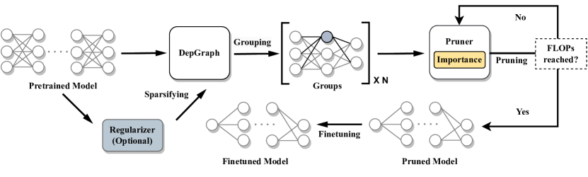
Figure 1: The framework of PruningBench, consisting of four steps: sparsifying, grouping, pruning and finetuning. Note that when benchmarking sparsifying regularizers (importance criteria), all other steps are fixed for fair comparisons.

Existing structural pruning literature mainly focuses on the sparsifying stage and the pruning stage. For sparsifying-stage methods, sparsity regularizers are proposed to learn structured sparse networks by imposing sparse constraints on loss functions and zeroing out certain weights. For pruning-stage methods, importance criteria are proposed to assess the importance of filters within a neural network, identifying redundant filters or channels that should be pruned. Note that importance criteria and sparsity regularizers are not mutually exclusive, suggesting that they can be utilized simultaneously to further promote the pruning performance. In this work, sparsifying-stage methods and pruning-stage methods are benchmarked separately.

3 PruningBench Settings

With the proposed PruningBench framework, we make a comprehensive study on existing structural pruning methods. We provide two leaderboards for each model-dataset combination, one for sparsifying-stage methods and the other for pruning-stage methods. The experimental settings in our benchmark are summarized as follows. For more details, please refer to the SUPP.

Models and Datasets. The benchmark now has been conducted on visual classification and detection tasks. For visual classification, we carry out the pruning experiments on the widely used CIFAR100 [51] and ImageNet [52] datasets, with ResNet18, ResNet50 [54], VGG19 [55] and ViT-small [49]. For visual detection, evaluations are conducted with YOLOv8 [50] on the COCO dataset [53]. The ResNet models for CIFAR100 are sourced from [56], and VGG models are sourced from [57]. For all these CIFAR models, the pretrained models used for pruning are trained by ourselves (see SUPP for the training details). For ImageNet experiments, the ResNet models and pretrained weights are obtained from the torchvision library [58], while the ViT-small model and its pretrained weight are sourced from the timm library [59]. For COCO experiments, the implementation and pretrained weight of the YOLOv8 model are obtained from the ultralytics library [60].

Pruning Methods. As aforementioned, PruningBench systematically evaluates $16$ existing pruning methods, including both the sparsifying-stage methods and the pruning-stage methods. For sparsifying-stage methods, we select GrowingReg [11], GroupNorm [15], GroupLASSO [61], and BNScale [26], where GrowingReg, GroupNorm and GroupLASSO are representatives of weight-based sparsity regularizers, and BNScale is a BN-based sparsity regularizer. Pruning-stage methods can be further categorized into data-free and data-driven methods. Data-free methods rely solely on weight information and produce deterministic results, whereas data-driven methods require input samples for pruning and yield non-deterministic results. In our benchmark, we select MagnitudeL1 [21], MagnitudeL2 [21], LAMP [23], FPGM [20], Random [22] and BNScale [26] as the representatives of the data-free methods, and CP [24], HRank [9], ThiNet [25], OBD-C [18], OBD-Hessian [15], and Taylor [19] as the representatives of the data-driven methods. Notably, for data-driven methods, we observe varying results due to varying input samples. To mitigate this randomness, we repeat the experiments three times to get the average results.

Performance Metrics. The performances of different pruning methods are evaluated at several predefined speedup ratios. On CIFAR100, the speedup ratios are defined as {$2$x, $4$x, $8$x}. For large datasets, COCO and ImageNet, where tasks become more complex and tolerable pruning decreases, we adopt the speedup ratios {$2$x, $3$x, $4$x}. At each speedup ratio, pruning methods are compared in metrics of accuracy, parameters, pruning time, and regularizing time if sparsity regularizers are used.

Pruning Schemes. Currently there exist two pruning schemes: local pruning and global pruning. Local pruning removes a consistent proportion of parameters for each group in the network [18, 20, 21, 22, 9, 24, 25, 27, 11]. However, as the importance and the redundancy of parameters across layers differ largely, a consistent pruning strategy is usually suboptimal. In contrast to local pruning, global pruning removes structures from all available structures of a network until a specific speedup ratio is reached [19, 15, 23, 13, 26, 15], without constraining the pruning ratio across different groups to be consistent. However, global pruning may prune the entire group at high speedup ratio, leaving the model functionality broken down. To address these issues, we propose protected global pruning in this benchmark , which preserves at least 10% of the parameters within each group with global pruning. Experiments demonstrate that protected global protection yields comparable results at low (e.g., $2$x) speedup ratio and significantly superior performance at high (e.g., $4$x and $8$x) speedup ratio. Experimental results and discussions are deferred to Section 4.

Hyperparameters. When evaluating pruning-stage methods (i.e., importance criteria), the sparsifying stage is skipped. All involved hyperparameters in the fine-tuning stage are fixed to be the same. For sparsifying-stage methods, however, evaluation becomes more complex. Sparsifying-stage methods still rely on importance criteria at the pruning stage. For CNN experiments, we employ MagnitudeL2 [21] and BNScale [26] when benchmark sparsifying-stage methods, which are proven to be stable and data-agnostic. However, for ViT experiments, we only use MagnitudeL2 due to the incompatibility of the ViT architecture with BNScale. Moreover, different sparsity regularizers have different hyperparameters, which are specific to each case and exhibit substantial differences across diverse model-dataset tasks. In our experiments, we carefully tune the hyperparameters individually for each sparsity regularizer. For more hyperparameters of sparsifying, pruning and finetuning stages, please refer to the SUPP.

4 Benchmark Results and Discussions

Table 2: The leaderboard of ResNet50 on CIFAR100 at three different speedup ratios, including rankings and the pruning results. “Step Time” indicates the time required for each pruning step, while “Reg Time” represents the time for each sparse learning epoch. An asterisk (*) indicates the importance criterion is random or data-driven that requires feature maps, gradients, etc., to calculate importance, exhibiting stochastic behavior.

Speed Up	Method
	Importance	Regularizer	Rank	Base	Pruned	$\Delta$ Acc	Pruning Ratio	Step Time	Reg Time
2x	OBD-C∗ [18]	N/A	1	78.35	78.68	+0.33	16.45 M (69.39%)	7.559s	N/A
	Taylor∗ [19]	N/A	2	78.35	78.51	+0.16	16.65 M (70.24%)	3.740s	N/A
	FPGM [20]	N/A	3	78.35	78.37	+0.02	15.37 M (64.84%)	0.163s	N/A
	MagnitudeL2 [21]	N/A	4	78.35	78.32	-0.03	16.63 M (70.17%)	0.136s	N/A
	BNScale [26]	N/A	5	78.35	78.30	-0.05	15.96 M (67.32%)	0.141s	N/A
	ThiNet∗ [25]	N/A	6	78.35	78.14	-0.21	15.19 M (64.06%)	33.619s	N/A
	Random∗ [22]	N/A	7	78.35	77.97	-0.38	11.78 M (49.70%)	0.104s	N/A
	CP∗ [24]	N/A	8	78.35	77.80	-0.55	7.15 M (30.15%)	2m51s	N/A
	MagnitudeL1 [21]	N/A	9	78.35	77.62	-0.73	16.91 M (71.34%)	0.137s	N/A
	OBD-Hessian∗ [15]	N/A	10	78.35	77.26	-1.09	7.83 M (33.03%)	5m5s	N/A
	LAMP [23]	N/A	11	78.35	76.26	-2.09	16.21 M (68.37%)	0.150s	N/A
	HRank∗ [9]	N/A	12	78.35	76.13	-2.22	6.47 M (27.29%)	34m32s	N/A
	MagnitudeL2 [21]	GroupLASSO [61]	1	78.35	78.73	+0.38	16.51 M (69.66%)	0.136s	3m5s
	BNScale [26]	BNScale [26]	2	78.35	78.36	+0.01	15.97 M (67.37%)	0.141s	2m14s
	MagnitudeL2 [21]	GroupNorm [15]	3	78.35	78.30	-0.05	15.03 M (63.41%)	0.136s	3m7s
	BNScale [26]	GroupLASSO [61]	4	78.35	78.24	-0.11	15.86 M (66.90%)	0.141s	2m38s
	MagnitudeL2 [21]	GrowingReg [11]	5	78.35	77.99	-0.36	16.61 M (70.06%)	0.136s	3m1s
4x	FPGM	N/A	1	78.35	78.02	-0.33	10.23 M (43.16%)	0.163s	N/A
	MagnitudeL2 [21]	N/A	2	78.35	77.98	-0.37	10.71 M (45.19%)	0.136s	N/A
	BNScale [26]	N/A	3	78.35	77.90	-0.45	10.53 M (44.41%)	0.141s	N/A
	MagnitudeL1 [21]	N/A	4	78.35	77.82	-0.53	11.10 M (46.81%)	0.137s	N/A
	Taylor∗ [19]	N/A	5	78.35	77.69	-0.66	5.47 M (23.09%)	3.740s	N/A
	OBD-C∗ [18]	N/A	6	78.35	77.51	-0.84	5.84 M (24.64%)	7.559s	N/A
	Random∗ [22]	N/A	7	78.35	77.41	-0.94	5.95 M (25.11%)	0.104s	N/A
	ThiNet∗ [25]	N/A	8	78.35	77.23	-1.12	4.72 M (19.91%)	33.619s	N/A
	CP∗ [24]	N/A	9	78.35	75.68	-2.67	2.65 M(11.18%)	2m51s	N/A
	LAMP [23]	N/A	10	78.35	75.52	-2.83	5.93 M (25.03%)	0.150s	N/A
	OBD-Hessian∗ [15]	N/A	11	78.35	75.49	-2.86	3.26 M (13.75%)	5m5s	N/A
	HRank∗ [9]	N/A	12	78.35	73.76	-4.59	1.69 M(7.11%)	34m32s	N/A
	BNScale [26]	BNScale [26]	1	78.35	78.16	-0.19	10.37 M (43.75%)	0.141s	2m14s
	MagnitudeL2 [21]	GroupLASSO [61]	2	78.35	78.01	-0.34	10.79 M (45.53%)	0.136s	3m5s
	BNScale [26]	GroupLASSO [61]	3	78.35	77.90	-0.45	10.76 M (45.38%)	0.141s	2m38s
	MagnitudeL2 [21]	GroupNorm [15]	4	78.35	77.88	-0.47	9.84 M (41.51%)	0.136s	3m7s
	MagnitudeL2 [21]	GrowingReg [11]	5	78.35	77.86	-0.49	10.77 M (45.43%)	0.136s	3m1s
8x	MagnitudeL1 [21]	N/A	1	78.35	76.99	-1.36	6.82 M (28.77%)	0.137s	N/A
	MagnitudeL2 [21]	N/A	2	78.35	76.38	-1.97	6.89 M (29.05%)	0.136s	N/A
	Random∗ [22]	N/A	3	78.35	76.13	-2.22	2.98 M (12.57%)	0.104s	N/A
	FPGM	N/A	4	78.35	75.93	-2.42	7.16 M (30.20%)	0.163s	N/A
	BNScale [26]	N/A	5	78.35	75.81	-2.54	6.69 M (28.22%)	0.141s	N/A
	OBD-C∗ [18]	N/A	6	78.35	75.78	-2.57	2.35 M (9.92%)	7.559s	N/A
	Taylor∗ [19]	N/A	7	78.35	75.38	-2.97	1.98 M (8.34%)	3.740s	N/A
	ThiNet∗ [25]	N/A	8	78.35	75.29	-3.06	1.58 M (6.68%)	33.619s	N/A
	OBD-Hessian∗ [15]	N/A	9	78.35	74.49	-3.86	1.66 M (7.02%)	5m5s	N/A
	LAMP [23]	N/A	10	78.35	73.48	-4.87	3.62 M (15.27%)	0.150s	N/A
	CP∗ [24]	N/A	11	78.35	72.39	-5.96	0.97 M (4.07%)	2m51s	N/A
	HRank∗ [9]	N/A	12	78.35	70.54	-7.81	0.64 M (2.69%)	34m32s	N/A
	MagnitudeL2 [21]	GrowingReg [11]	1	78.35	76.39	-1.96	7.00 M (29.52%)	0.136s	3m1s
	MagnitudeL2 [21]	GroupLASSO [61]	2	78.35	76.27	-2.08	7.09 M (29.90%)	0.136s	3m5s
	MagnitudeL2 [21]	GroupNorm [15]	3	78.35	75.93	-2.42	7.18 M (30.28%)	0.136s	3m7s
	BNScale [26]	GroupLASSO [61]	4	78.35	75.60	-2.75	7.19 M (30.32%)	0.141s	2m38s
	BNScale [26]	BNScale [26]	5	78.35	75.47	-2.88	6.90 M (29.12%)	0.141s	2m14s

Table 3: The leaderboard of ViT-small on ImageNet at three different speedup ratios.

Speed Up	Method
	Importance	Regularizer	Rank	Base	Pruned	$\Delta$ Acc	Parameters	Step Time	Reg Time
2x	FPGM [20]	N/A	1	78.588	69.248	-9.34	10.365 M (47.01%)	0.937s	N/A
	Random∗ [22]	N/A	2	78.588	68.810	-9.778	9.305 M (42.20%)	0.888s	N/A
	LAMP [23]	N/A	3	78.588	68.724	-9.864	10.169 M (46.12%)	1.284s	N/A
	MagnitudeL1 [21]	N/A	4	78.588	68.602	-9.986	10.375 M (47.05%)	1.005s	N/A
	MagnitudeL2 [21]	N/A	5	78.588	68.316	-10.272	10.346 M (46.92%)	0.995s	N/A
	OBD-Hessian∗ [15]	N/A	6	78.588	67.514	-11.074	10.334 M (46.87%)	6m40s	N/A
	Taylor∗ [19]	N/A	7	78.588	67.400	-11.188	10.468 M (47.47%)	27.634s	N/A
	CP∗ [24]	N/A	7	78.588	67.400	-11.188	10.334 M (46.87%)	15m4s	N/A
	ThiNet∗ [25]	N/A	8	78.588	63.914	-14.674	6.439 M (29.20%)	3m17s	N/A
	MagnitudeL2 [21]	GrowingReg [11]	1	78.588	68.715	-9.873	10.359 M (46.98%)	0.995s	5h10m31s
	MagnitudeL2 [21]	GroupNorm [15]	2	78.588	68.594	-9.994	10.363 M (47.00%)	0.995s	5h21m21s
	MagnitudeL2 [21]	GroupLASSO [61]	3	78.588	68.350	-10.238	10.360 M (46.98%)	0.995s	5h15m13s
3x	MagnitudeL1 [21]	N/A	1	78.588	63.120	-15.468	6.57 M (29.79%)	1.005s	N/A
	LAMP [23]	N/A	2	78.588	62.538	-16.050	6.08 M (27.57%)	1.284s	N/A
	MagnitudeL2 [21]	N/A	3	78.588	62.342	-16.246	6.37 M (28.89%)	0.995s	N/A
	Taylor∗ [19]	N/A	4	78.588	61.582	-17.006	6.62 M (30.01%)	27.634s	N/A
	FPGM [20]	N/A	5	78.588	60.660	-17.928	5.701 M (25.85%)	0.937s	N/A
	CP∗ [24]	N/A	6	78.588	56.626	-21.962	6.778 M (30.74%)	15m4s	N/A
	OBD-Hessian∗ [15]	N/A	7	78.588	54.796	-23.792	6.39 M (28.98%)	6m40s	N/A
	ThiNet∗ [25]	N/A	8	78.588	49.654	-28.934	5.113 M (23.19%)	3m17s	N/A
	Random∗ [22]	N/A	9	78.588	44.654	-33.954	4.95 M (22.45%)	0.888s	N/A
	MagnitudeL2 [21]	GrowingReg [11]	1	78.588	62.608	-15.980	6.57 M (29.81%)	0.995s	5h10m31s
	MagnitudeL2 [21]	GroupNorm [15]	2	78.588	61.716	-16.872	6.88 M (31.20%)	0.995s	5h21m21s
	MagnitudeL2 [21]	GroupLASSO [61]	3	78.588	61.340	-17.248	6.57 M (29.13%)	0.995s	5h15m13s
4x	MagnitudeL1 [21]	N/A	1	78.588	59.950	-18.638	5.06 M (22.93%)	1.005s	N/A
	MagnitudeL2 [21]	N/A	2	78.588	59.082	-19.506	4.89 M (22.15%)	0.995s	N/A
	Taylor∗ [19]	N/A	3	78.588	57.650	-20.938	4.80 M (21.76%)	27.634s	N/A
	LAMP [23]	N/A	4	78.588	55.750	-22.838	4.32 M (19.57%)	1.284s	N/A
	FPGM [20]	N/A	5	78.588	48.258	-30.33	3.25 M (14.74%)	0.937	N/A
	OBD-Hessian∗ [15]	N/A	6	78.588	36.600	-41.988	4.25 M (19.27%)	6m40s	N/A
	CP∗ [24]	N/A	7	78.588	42.574	-36.014	5.253 M (23.82%)	15m4s	N/A
	ThiNet∗ [25]	N/A	8	78.588	28.422	-50.166	2.669 M (12.10%)	3m17s	N/A
	Random∗ [22]	N/A	9	78.588	27.722	-50.866	2.76 M (12.54%)	0.888s	N/A
	MagnitudeL2 [21]	GrowingReg [11]	1	78.588	59.630	-18.958	4.56 M (20.66%)	0.995s	5h10m31s
	MagnitudeL2 [21]	GroupLASSO [61]	2	78.588	57.312	-21.276	4.59 M (20.81%)	0.995s	5h15m13s
	MagnitudeL2 [21]	GroupNorm [15]	3	78.588	56.446	-22.142	4.77 M (21.62%)	0.995s	5h21m21s

PruningBench now has completed $645$ model pruning experiments (i.e., getting $645$ pruned models), yielding $13$ leaderboards (9 on CIFAR, 3 on ImageNet, and one on COCO). For space considerations, here we present the leaderboard results of ResNet50 on CIFAR100 in Table 2, and the leaderboard results of ViT-small on ImageNet in Table 3. For more leaderboards, please refer to Table A3 to A15 in SUPP or our benchmark website at http://pruning.vipazoo.cn.

4.1 Benchmark Results

Overall Results. In general, no single methods consistently outperform the others across all settings and tasks. Nonetheless, weight norm-based methods, such as MagnitudeL1 and MagnitudeL2, typically exhibit superior performance and yield more reliable results, ranking within the top $5$ in most rankings while maintaining computational efficiency. This is followed by BNScale, FPGM, Taylor, and OBD-C, which also show commendable results in various scenarios. Other methodologies may not exhibit significant overall advantages, but may perform well in specific situations. Now we provide more detailed analyses of the leaderboard results by answering the following questions.

Q1: What is the impact of the model architectures on the leaderboard rankings?

Observation: BNScale, Hrank, and LAMP demonstrate clear architectural preferences. BNScale consistently ranks within the top five in most rankings for CNNs utilizing residual blocks (such as ResNet18, ResNet50, and YOLOv8), yet its efficacy notably diminishes when applied to VGG, where it typically ranks between 7th and 9th. In contrast, LAMP and Hrank display subpar performance on ResNet models, but showcase excellence on VGG, frequently ranking within the top 5. LAMP also demonstrates robust performance on ViT and YOLO, often ranking between 1st and 4th. While other pruning techniques exhibit some variability in performance across diverse architectures, they do not manifest strong architectural preferences.

Q2: What is the impact of the speedup ratio on the leaderboard rankings?

Observation: Different methods can exhibit varying rankings under different speedup ratios. MagnitudeL1, MagnitudeL2, BNScale, and LAMP slightly improve in ranking as the speedup ratio increases, indicating a certain level of pruning resilience. Conversely, FPGM, ThiNet, and Hrank tend to experience a decline in rankings as the speedup ratio increases. OBD-Hessian and CP methods show relatively stable performance, with minimal ranking shifts across speedup ratios. Taylor and OBD-C, however, display more erratic behavior, with their rankings sometimes significantly rising or falling depending on the architecture and speedup ratios.

Table 4: Results of ResNet50 pruned by MagnitudeL2 importance with three pruning schemes.

Speed Up	Prune Strategy	Base	Pruned	$\Delta$ Acc	Parameters
2x	global+protect	76.128	73.684	-2.444	18.26 M (71.44%)
	global prune	76.128	73.028	-3.100	18.43 M (72.12%)
	local prune	76.128	70.984	-5.144	12.99 M (50.85%)
3x	global+protect	76.128	71.805	-4.323	14.37 M (56.23%)
	global prune	76.128	63.486	-12.642	14.20 M (55.57%)
	lobal prune	76.128	69.168	-6.96	8.77 M (34.31%)
4x	global+protect	76.128	69.866	-6.262	11.88 M (46.49%)
	global prune	76.128	56.068	-20.06	12.38 M (48.46%)
	local prune	76.128	66.050	-10.078	6.63 M (25.94%)

Q3: Which methods are more efficient in terms of computation time?

Observation: Obviously, sparsifying-stage methods are significantly more computation expensive than pruning-stage methods due to the cumbersome sparse learning process. In general, in our experiments sparsifying-stage methods takes about $1.33\sim 2$ times longer time than pruning-stage methods. For pruning-stage methods, data-driven importance criteria [13, 24, 18, 9, 19, 25, 22, 62, 15], particularly those involving non-parallel operations [9, 15, 24, 25], consume longer pruning time compared to data-free methods. For example, OBD-Hessian [15] computes gradients separately for each sample. Thinet [25] and HRank [9] determine the importance of each output channel of each layer individually. These techniques are well-suited for one-shot pruning, where importance scores are calculated only once, followed by pruning the network to achieve the target pruning ratio. However, when applied to iterative pruning, the computation time increases significantly as the importance scores need to be calculated every iteration.

Q4: How do sparsity regularizers improve the performance of prunned model?

Observation: Sparsity regularizers [11, 15, 26, 61] aim to induce sparsity in network parameters, rendering redundant parameters proximate to zero or outright zero, thereby facilitating pruning based on importance criteria. However, in practical applications, we find that sparsity regularizers do not necessarily improve performance and only show significant effects in specific scenarios. Notably, across all experiments utilizing sparsity regularizers (refer to Table A3-A15 in the SUPP), only $57.30\%$ showcase positive performance improvements with sparsity regularization. Among these techniques, BNScale delivers the most favorable outcomes, with a $77.78\%$ probability of enhancing performance, followed by GroupLASSO with a $65.38\%$ likelihood of improvement. Conversely, GroupNorm and GrowingReg demonstrate lower effectiveness overall, with improvement probabilities of $42.31\%$ and $45.83\%$, respectively. Nonetheless, these methods excel in particular architectural settings. GrowingReg, for instance, excels in the ViT architecture, manifesting notable performance enhancements across all speedup ratios, while other techniques improve ViT performance less than half of the time. GroupNorm, on the other hand, is better suited for VGG models, exhibiting a $66.67\%$ probability of performance enhancement, a significant improvement compared to its performance in other architectures. A drawback of sparsity regularizers is the necessity for meticulous tuning tailored to each scenario, i.e., the optimal hyperparameters vary across diverse model-dataset configurations. Please refer to the SUPP for more details of the hyperparameters.

Q5: How consistent are the CIFAR rankings with the ImageNet rankings?

Observation: In comparison to pruning CIFAR100-trained models, pruning ImageNet-trained models (of the same architecture as CIFAR100-trained ones) typically results in more accuracy deterioration. Meanwhile, ImageNet-trained models are more sensitive to the speedup ratios. However, for the same model architecture, the leaderboard rankings on CIFAR are highly consistent with that on ImageNet (see Table A5, A8, A13-14 in SUPP for details). For example, when pruning ResNet models, MagnitudeL1, MagnitudeL2, BNScale, and Taylor methods consistently rank within the top five on both CIFAR100 and ImageNet, whereas LAMP and Hrank consistently rank low on the list. These observations indicate that pruning methods showcase a degree of consistency across datasets with the same model. In situations where computational resources are constrained, the utilization of smaller datasets for assessing pruning methodologies, followed by the application of the top-ranked techniques to prune larger models, emerges as a viable approach.

4.2 More Discussions

Local pruning, global pruning versus protected global pruning. Table 4 presents the results of ResNet50 pruned by MagnitudeL2 on ImageNet, with the three pruning schemes. Results on more models are provided in SUPP. From these results, we make the following two conclusions. (1) At low speedup ratios, global pruning and the proposed protected global pruning exhibit comparable performance, both surpassing local pruning. It can be attributed to the assumption in local pruning, which assigns equal importance to each group and applies the same pruning ratio to each group, overlooking group differences. To address this, some previous works such as [63, 21, 25, 13] propose sensitivity analysis in order to estimate the pruning ratio that should be applied to particular layers [19]. (2) In contrast, at higher speedup ratios, protected global pruning outperforms both local pruning and global pruning. An examination of the network architecture after global pruning uncover instances of layer collapse, where nearly all channels of a network layer are eliminated, rendering the network untrainable and severely impairing performance.

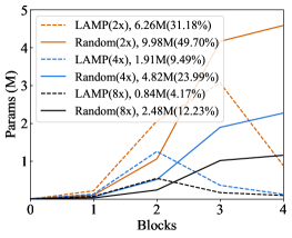
(a) Parameter curves on VGG19.

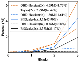
(b) Parameter curves on ResNet18.

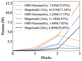
(c) Parameter curves on ResNet50.

Figure 2: The parameter curves of different models pruned by different importance criteria on CIFAR100 dataset. Details can be referred to in Tables A5, A8, and A11 in the SUPP.

Parameters versus FLOPS. Some prior works [10, 23, 41, 42, 43, 44, 45, 28, 29] employ the number of parameters as the performance metric of pruned models. Here we discuss the correlation between parameters and the computation cost, i.e., FLOPS. As evidenced in Table 2 and 3, different methods may yield significantly different numbers of pruned parameters at the identical speedup ratios, indicating unequal contributions of various parameters to the computational overhead. Specifically, as depicted in Figure 2, at the same speedup ratio, models with fewer total parameters have more parameters in their initial blocks. Here we provide a brief theoretical insight on this phenomenon. For a convolutional layer $\mathbf{W}\in\mathbb{R}^{\hat{N}NK^{2}}$, the input tensor $\mathbf{I}\in\mathbb{R}^{NHW}$, and the output tensor $\mathbf{O}\in\mathbb{R}^{\hat{N}\hat{H}\hat{W}}$, the computational complexity of this layer can be denoted by $\mathbf{I}$ is $O(N\hat{N}\hat{H}\hat{W}{K}^{2})$. The average computational contribution of each parameter is thus $O(\hat{H}\hat{W})$, which implies a positive linear correlation between the computation overhead and the feature map resolution. As CNN models usually progressively scale down the spatial resolution of feature maps as layers deepen, the method that prioritizes the reduction of shallow parameters can effectively decrease computational costs while minimizing the parameter count. However, the same method can exhibit varying preferences when pruning different architectures. For example, OBD-Hessian removes numerous parameters when pruning ResNet18 and ResNet50 (see Table 2 and Table A3 to Table A8 in SUPP), indicating a preference for pruning later layers. However, when pruning VGG19, it removes much fewer parameters, suggesting a focus on earlier layers (see Table A9 to Table A11 in SUPP).

CNNs versus ViTs. CNNs and ViTs present diverse characteristics and demonstrate distinct behavious in structural pruning. For instance, in the case of CNN architectures, owing to the aforementioned relationship between parameters and computational overhead, there can be large differences in the number of parameters pruned by different methods at the identical speedup ratios (see Table 2 and other CNN experiments in SUPP). However, for the ViT-small experiments in Table 3, the differences in the number of parameters among different methods at the same speedup ratio are small. This phenomenon arises from the fixed-shaped flattened tensors that characterize the output feature maps of ViT, ensuring a consistent contribution of parameters to computational overhead across distinct layers. Therefore, in contrast to CNN, using the number of parameters as the performance metric for pruning ViTs can also lead to reliable conclusions, thanks to the nearly linear correlation between parameters and computational cost.

Another crucial aspect of Vision Transformers (ViTs) is the intricate interconnection of the patch embedding layer with other layers. The output dimension of the patch embedding layer plays a pivotal role in determining the input dimension for all attention layers, making ViT pruning particularly sensitive to this layer. Additionally, ViT necessitates pruning same dimensions for different attention heads, thereby increasing the implementation complexity. Moreover, in comparison to ResNet50, ViT-small, with a similar model size, suffer from more accuracy loss. As depicted in Table 5, at the same speedup ratio, the accuracy loss of ViT-small is several times greater than that of ResNet50. The experimental result aligns with the general consensus in prior literature [64, 65, 66, 67, 68] that ViT models are harder to compress while preserving accuracy compared to their classic convolutional counterparts. For further comparisons, please consult Table 3 and Table A14 in the SUPP.

Table 5: Results of MagnitudeL2 with different speedup ratios on ImageNet and CIFAR100.

Dataset	Model	Speed Up	Base	Pruned	$\Delta$ Acc	Dataset	Model	Speed Up	Base	Pruned	$\Delta$ Acc
ImageNet	ViT-Small (22.05M)	2x	78.588	68.316	-10.272	CIFAR100	VGG19 (20.09M)	2x	73.87	73.22	-0.65
		3x	78.588	62.342	-16.246			4x	73.87	71.95	-1.92
		4x	78.588	59.282	-19.506			8x	73.87	64.96	-8.91
	ResNet-50 (25.56M)	2x	76.128	73.684	-2.444		ResNet-50 (23.70M)	2x	78.35	78.32	-0.03
		3x	76.128	71.805	-4.323			4x	78.35	77.98	-0.37
		4x	76.128	69.866	-6.262			8x	78.35	76.38	-1.97
	ResNet-18 (11.69M)	2x	69.758	67.502	-2.256		ResNet-18 (11.23M)	2x	75.61	75.72	+0.11
		3x	69.758	63.284	-6.474			4x	75.61	74.01	-1.60
		4x	69.758	60.438	-9.32			8x	75.61	71.87	-3.74

Method applicability. The applicability of different pruning methods exhibits considerable variance. Most methods are tailored for CNNs, presenting obstacles when adapting them to alternative architectural designs. For instance, HRank [9] determines channel importance based on the rank of feature map corresponding to each channel, which is incompatible with architectures like ViTs. Since ViTs output flattened tensors, pruning through this method is unfeasible. Analogous challenges emerge with Batch Normalization (BN)-based techniques [26, 37, 38, 30, 39], which rely on batch normalization layers for importance score. Consequently, these methods can not be directly applied to architectures without batch normalization layers. In contrast to the previously mentioned approaches, techniques based on weight normalization [21, 69, 23] and weight similarity [20, 70, 48, 32, 33] exhibit minimal constraints and can be seamlessly integrated into diverse architectural frameworks.

5 Conclusion and Future Work

In this work, we present to our best knowledge the first comprehensive structural pruning benchmark, PruningBench. PruningBench systematically evaluates 16 existing structural pruning methods on a wide array of models and tasks, yielding a handful of interesting findings which are not explored previously. Furthermore, PruningBench is designed as an expandable package that standardizes experimental settings and eases the integration of new algorithmic implementations. In the future work, we will make a more broader study on structural pruning evaluation, covering more advanced models like language models, diffusion models, GNNs, etc.

6 Supplementary Material

6.1 Related work

PruningBench categorizes current structural pruning methods into importance criteria and sparsity regularizers. Importance criteria assess the importance of filters within a neural network, identifying redundant filters or channels that need to be pruned, whereas sparsity regularizers aim to learn structured sparse networks by imposing sparse constraints on loss functions and zeroing out certain weights during training.

The sparsity regularizers can be applied to Batch Normalization (BN) parameters [71] if the networks contain batch normalization layers [26, 37, 38, 30], and then the BN parameters are used to indicate the pruning decision of structures such as channels or filters. Sparsity regularizers can also be directly applied to filters [71, 11, 15, 61, 27]. Group Lasso regularization [61, 27] is commonly used to sparsify filters in a structured manner. Growing Regularization (GREG) [11] exploits regularization under a growing penalty and uses two algorithms. More recently, GroupNorm [15] promotes sparsity across all grouped layers, convering convolutions, batch normalizations and fully-connected layers.

Importance criteria can be divided into two approaches: data-free methods and data-driven methods. Data-free methods rely solely on the existing weight information of the network and do not depend on input data, making their pruning results deterministic. These methods can be classified into four categories: weight-norm, weight-correlation, BN-based, and random. Weight-norm methods [21, 23, 69] prune based on the norms of weight values. Representative works, such as MagnitudeL1 [21], MagnitudeL2 [21], and LAMP [23], consider filters with smaller norms to have weak activation, thus contributing less to the final classification decision [71]. Weight-correlation methods [20, 32, 33, 48, 70] prune based on the relationships between weight values. For instance, FPGM identifies filters close to the geometric median to be redundant, as they represent common information shared by all filters in the same layer and should be removed. BN-based methods [11, 15, 61, 27] prune based on the weights of BN layers. BNScale [26] directly uses the scaling parameter $\gamma$ of the BN layer to compute the importance scores, while Kang et al. [39] also consider shifting parameters $\beta$. Random methods [22] perform pruning in a random manner.

In contrast, data-driven methods are pruning techniques that require input samples, making their results non-deterministic and dependent on the quality of the input data. These methods can be categorized into activation-based and gradient-based approaches. Activation-based methods [24, 9, 25, 45, 34, 28, 29] utilize activation maps for pruning. For example, CP [24] and HRank [9] evaluate channel importance of current layer using reconstruction error [24] and activation map decomposition [9], respectively. ThiNet [25], on the other hand, uses activation maps from the next layer to guide the pruning of the current layer. Gradient-based methods [18, 15, 19, 62, 72] rely on gradients or Hessian information to perform pruning. Methods that rely solely on gradients, such as Taylor-FO [19] and Mol-16 [36], can obtain importance scores from backpropagation without requiring additional memory. Conversely, hessian-based methods, such as OBD-Hessian [15] and OBD-C [18], require calculating second-order derivatives, which are computationally prohibitive.

6.2 Hyperparameters

Table 1: The performance under different pruning steps on the CIFAR100 dataset, including accuracy change, parameter count and FLOPs. The experiments aim to yield a fourfold speedup (i.e., maintaining 25% of the original FLOPs) for ResNet18.

Method	Steps	Base	Pruned	$\Delta$ Acc	Parameters	FLOPs
BNScale [26]	10	75.60	72.90	-2.7	3.08 M (27.48%)	93.57 M (16.81%)
	50	75.60	74.00	-2.06	5.03 M (44.84%)	135.84 M (24.40%)
	400	75.60	73.68	-1.92	5.15 M (45.90%)	137.45 M (24.69%)
MagnitudeL2 [21]	10	75.60	73.36	-2.24	3.19 M (28.42%)	102.98 M (18.50%)
	50	75.60	74.44	-1.66	4.34 M (38.72%)	138.05 M (24.80%)
	400	75.60	74.01	-1.59	4.43 M (39.51%)	138.65 M (24.91%)

6.2.1 Pruning Step

A larger pruning step value allows for finer control over FLOPs. Table 1 demonstrates that setting the pruning step to 10 often results in excessive pruning, leading to FLOPs significantly below the target and a corresponding decrease in accuracy. While the accuracy changes are similar for pruning steps set to 50 and 400, the latter offers more precise FLOPs control. Therefore, we chose 400 pruning steps for the leaderboard experiments.

6.2.2 Hyperparameters of Pretraining

As mentioned in the main text, the models for the CIFAR100 experiments are pretrained by us, while the experiments on other datasets utilize publicly available pretrained weights. For the CIFAR100 CNN experiments, we pretrain the models (ResNet18, ResNet50, VGG19) for 200 epochs using SGD with an initial learning rate of 0.1. The learning rate decreases by a factor of 10 at the 120th, 150th, and 180th epochs. We set the batch size to 128 and the weight decay to $5\times 10^{-4}$.

6.2.3 Hyperparameters of Finetuning Stage

CNN experiments. For the CNN experiments on CIFAR100, we use SGD with an initial learning rate of 0.01. The learning rate is reduced to one-tenth of its original value every 20 epochs after 60 epochs, until fine-tuning concludes at the 100th epochs. We set the batch size to 128, the weight decay to $5\times 10^{-4}$, and the Nesterov momentum to 0.9. For the CNN experiments on ImageNet, we adjust the learning rate to 0.1 and the weight decay to $1\times 10^{-4}$. The learning rate is reduced by a factor of 10 at the 30th and 60th epochs, with fine-tuning concluding at the 90th epochs.

ViT-small experiments. For ViT-small experiments on ImageNet, we adopt AdamW as the optimizer. The batch size is set to 128 and the weight decay to 0.3. Various data augmentation techniques, as mentioned by Touvron et al. [73], are employed. Due to the slow convergence and sensitivity to the learning rate of ViT-small, we use different learning rates for different speedup ratios. Specifically, for a speedup ratio of 2, the learning rate is set to $1.5\times 10^{-5}$, while for speedup ratios of 3 and 4, the learning rate is set to $1.5\times 10^{-4}$. The cosine annealing schedule is used for learning rate decay and the fine-tuning finishes at the 90th epochs.

YOLOv8 experiments. For YOLOv8 experiments on COCO, we utilize SGD with a learning rate of 0.01. The learning rate scheduler initiates a warmup phase followed by linear decay until the completion of fine-tuning at the 100th epoch. We configure the batch size to 128, the weight decay to $5\times 10^{-4}$, and the Nesterov momentum to 0.937.

6.2.4 Hyperparameters of Sparsifying Stage.

Sparsity regularizers require case-by-case tuning of their hyperparameters for optimal sparse learning. Table 2 presents the optimal hyperparameters across different tasks. Other hyperparameters, such as epoches, batch size and weight decay, are consistent with those used in the finetuning stage.

Table 2: The optimal hyperparameters for the sparsity regularizers across different tasks. $\lambda$ denotes the regularization coefficient, $\eta$ is the learning rate for sparse learning, and $\delta$ is the delta coefficient in GrowingReg [11]. ${*}$ indicates that the $\eta$ value for the ViT-small model is identical to the learning rate used during its finetuning stage and is adjusted based on the speedup ratio.

Method	Task
	Model	Dataset	$\lambda$	$\eta$	$\delta$
GroupLASSO [61] (for MagnitudeL2)	VGG19	CIFAR100	0.00001	0.001	–
	ResNet18	CIFAR100	0.0005	0.005	–
	ResNet50	CIFAR100	0.0001	0.005	–
	ResNet18	ImageNet	0.00005	0.005	–
	ResNet50	ImageNet	0.0005	0.01	–
	ViT-small	ImageNet	0.0001	${*}$	–
	YOLOv8	COCO	0.0001	0.001	–
GroupLASSO [61] (for BNScale)	VGG19	CIFAR100	0.0005	0.005	–
	ResNet18	CIFAR100	0.00005	0.01	–
	ResNet50	CIFAR100	0.00005	0.01	–
	ResNet18	ImageNet	0.0005	0.005	–
	ResNet50	ImageNet	0.0005	0.01	–
	ViT-small	ImageNet	0.0001	${*}$	–
	YOLOv8	COCO	0.0005	0.001	–
GroupNorm [15] (for MagnitudeL2)	VGG19	CIFAR100	0.00001	0.005	–
	ResNet18	CIFAR100	0.0001	0.005	–
	ResNet50	CIFAR100	0.0001	0.005	–
	ResNet18	ImageNet	0.00005	0.01	–
	ResNet50	ImageNet	0.0005	0.005	–
	ViT-small	ImageNet	0.0005	${*}$	–
	YOLOv8	COCO	0.0001	0.01	–
BNScale [26] (for BNScale)	VGG19	CIFAR100	0.0005	0.005	–
	ResNet18	CIFAR100	0.0001	0.01	–
	ResNet50	CIFAR100	0.00001	0.01	–
	ResNet18	ImageNet	0.0001	0.01	–
	ResNet50	ImageNet	0.00005	0.01	–
	YOLOv8	COCO	0.00001	0.005	–
GrowingReg [11] (for MagnitudeL2)	VGG19	CIFAR100	0.0001	0.001	0.00001
	ResNet18	CIFAR100	0.0005	0.01	0.0001
	ResNet50	CIFAR100	0.0001	0.001	0.00001
	ResNet18	ImageNet	0.0001	0.005	0.00005
	ResNet50	ImageNet	0.00005	0.01	0.00001
	ViT-small	ImageNet	0.0005	${*}$	0.0001
	YOLOv8	COCO	0.0001	0.005	0.00005

6.3 Unified Interfaces

6.3.1 Interface for Importance Criteria.

PruningBench categorizes the network layers, where each kind of layer requires a different pruning scheme, corresponding to different importance criteria interfaces that users should implement. Because of the interdependencies among these layers, pruning parameters in one layer necessitates the simultaneous pruning of parameters in other layers that depend on it. Thus, users only need to implement a part of the interfaces based on their algorithm, and PruningBench will extend pruning to the entire group. PruningBench classifies the network layers into the following types:

convolutional input and output layers. For a convolutional layer $\mathbf{W}\in\mathbb{R}^{\hat{N}NK^{2}}$ and $\mathbf{b}\in\mathbb{R}^{\hat{N}}$ (where $\mathbf{W}$ represents the weights and $\mathbf{b}$ is the bias), the input tensor $\mathbf{I}\in\mathbb{R}^{NHW}$, and the output tensor $\mathbf{O}\in\mathbb{R}^{\hat{N}\hat{H}\hat{W}}$. In a convolutional output layer, the output channels (filters) are pruned, with the pruning scheme represented by $\mathbf{W}[k,:,:,:]$ and $\mathbf{b}[k]$. In this context, the importance criteria interface that should be implemented by users is $I(\mathbf{W})\in\mathbb{R}^{\hat{N}}$, where each element of $I(\mathbf{W})$ signifies the importance score of parameters along the first dimension of $\mathbf{W}$. PruningBench selects indices for pruning based on $I(\mathbf{W})$ and removes them accordingly. Subsequently, PruningBench prunes $\mathbf{b}[k]$ and parameters in other layers that are coupled with it. In contrast, in a convolutional input layer, the input channels are pruned, with the pruning scheme denoted as $\mathbf{W}[:,k,:,:]$ (the bias remains unaffected), which implies the second dimension of $\mathbf{W}$ should be pruned.

linear input and output layers. A linear layer can be parameterized as $\{\mathbf{W}\in\mathbb{R}^{\hat{N}N},\mathbf{b}\in\mathbb{R}^{\hat{N}}\}$. Same to convolutional input and output layers. linear layers have distinct pruning schemes for their inputs and outputs, i.e., $\mathbf{W}[k,:]$ and $\mathbf{b}[k]$ for output layers and $\mathbf{W}[:,k]$ for input layers.

Table 3: Leaderboard of ResNet50 on CIFAR100 at three different speedup ratios. Global pruning strategy is adapted.

Speed Up	Method
	Importance	Regularizer	Rank	Base	Pruned	$\Delta$ Acc	Pruning Ratio	Step Time	Reg Time
2x	OBD-C∗ [18]	N/A	1	78.35	78.67	+0.32	16.64 M (70.19%)	7.471s	N/A
	MagnitudeL1 [21]	N/A	2	78.35	78.36	+0.01	16.98 M (71.62%)	0.137s	N/A
	FPGM [20]	N/A	3	78.35	78.32	-0.03	15.18 M (64.04%)	0.163s	N/A
	MagnitudeL2 [21]	N/A	4	78.35	78.20	-0.15	16.62 M (70.10%)	0.136s	N/A
	ThiNet∗ [25]	N/A	4	78.35	78.20	-0.15	16.64 M (70.19%)	33.516s	N/A
	BNScale [26]	N/A	5	78.35	78.07	-0.28	15.96 M (67.32%)	0.140s	N/A
	Taylor∗ [19]	N/A	6	78.35	77.92	-0.43	16.62 M (70.11%)	3.725s	N/A
	Random∗ [22]	N/A	7	78.35	77.72	-0.63	11.82 M (49.88%)	0.104s	N/A
	CP∗ [24]	N/A	8	78.35	77.53	-0.82	7.09 M (29.93%)	2m51s	N/A
	HRank∗ [9]	N/A	9	78.35	77.31	-1.04	7.53 M (31.76%)	34m30s	N/A
	OBD-Hessian∗ [15]	N/A	10	78.35	77.07	-1.28	7.64 M (32.21%)	5m5s	N/A
	LAMP [23]	N/A	11	78.35	75.44	-2.91	16.23 M (68.46%)	0.151s	N/A
	MagnitudeL2 [21]	GroupLASSO [61]	1	78.35	78.49	+0.14	16.20 M (68.35%)	0.136s	3m5s
	MagnitudeL2 [21]	GrowingReg [11]	2	78.35	78.38	+0.03	16.21 M (68.39%)	0.136s	3m1s
	BNScale [26]	BNScale [26]	3	78.35	78.22	-0.13	16.85 M (71.10%)	0.140s	2m14s
	MagnitudeL2 [21]	GroupNorm [15]	4	78.35	78.05	-0.30	15.10 M (63.71%)	0.136s	3m7s
	BNScale [26]	GroupLASSO [61]	5	78.35	77.97	-0.38	16.25 M (68.55%)	0.140s	2m38s
4x	BNScale [26]	N/A	1	78.35	78.11	-0.24	10.50 M (44.31%)	0.140s	N/A
	MagnitudeL1 [21]	N/A	2	78.35	78.02	-0.33	11.12 M (46.91%)	0.137s	N/A
	MagnitudeL2 [21]	N/A	3	78.35	77.67	-0.68	10.76 M (45.39%)	0.136s	N/A
	FPGM [20]	N/A	4	78.35	77.63	-0.72	9.98 M (42.11%)	0.163s	N/A
	Taylor∗ [19]	N/A	5	78.35	77.50	-0.85	5.46 M (23.02%)	3.725s	N/A
	ThiNet∗ [25]	N/A	6	78.35	77.44	-0.91	5.23 M (22.07%)	33.516s	N/A
	OBD-C∗ [18]	N/A	7	78.35	77.32	-1.03	5.80 M (24.48%)	7.471s	N/A
	Random∗ [22]	N/A	8	78.35	77.05	-1.30	6.12 M (25.81%)	0.104s	N/A
	CP∗ [24]	N/A	9	78.35	75.78	-2.57	2.54 M (10.71%)	2m51s	N/A
	OBD-Hessian∗ [15]	N/A	10	78.35	75.33	-3.02	3.38 M (14.26%)	5m5s	N/A
	LAMP [23]	N/A	11	78.35	74.32	-4.03	6.24 M (26.33%)	0.151s	N/A
	HRank∗ [9]	N/A	12	78.35	72.06	-6.29	1.63 M (6.87%)	34m30s	N/A
	BNScale [26]	BNScale [26]	1	78.35	77.79	-0.56	10.74 M (45.30%)	0.140s	2m14s
	MagnitudeL2 [21]	GrowingReg [11]	2	78.35	77.73	-0.62	10.65 M (44.93%)	0.136s	3m1s
	BNScale [26]	GroupLASSO [61]	3	78.35	77.71	-0.64	10.73 M (45.25%)	0.140s	2m38s
	MagnitudeL2 [21]	GroupLASSO [61]	4	78.35	77.69	-0.66	10.67 M (45.02%)	0.136s	3m5s
	MagnitudeL2 [21]	GroupNorm [15]	5	78.35	77.48	-0.87	9.72 M (40.99%)	0.136s	3m7s
8x	MagnitudeL1 [21]	N/A	1	78.35	76.48	-1.87	7.00 M (29.52%)	0.137s	N/A
	BNScale [26]	N/A	2	78.35	76.31	-2.04	6.76 M (28.53%)	0.140s	N/A
	Random∗ [22]	N/A	3	78.35	76.12	-2.23	3.17 M (13.36%)	0.104s	N/A
	FPGM [20]	N/A	4	78.35	76.08	-2.27	6.68 M (28.18%)	0.163s	N/A
	MagnitudeL2 [21]	N/A	5	78.35	76.06	-2.29	7.06 M (29.78%)	0.136s	N/A
	OBD-C∗ [18]	N/A	6	78.35	75.44	-2.91	2.43 M (10.25%)	7.471s	N/A
	Taylor∗ [19]	N/A	7	78.35	75.41	-2.94	1.89 M (7.99%)	3.725s	N/A
	ThiNet∗ [25]	N/A	8	78.35	74.93	-3.42	1.54 M (6.48%)	33.516s	N/A
	OBD-Hessian∗ [15]	N/A	9	78.35	73.65	-4.70	1.33 M (5.60%)	5m5s	N/A
	LAMP [23]	N/A	10	78.35	73.01	-5.34	3.58 M (15.08%)	0.151s	N/A
	CP∗ [24]	N/A	11	78.35	72.61	-5.74	0.98 M (4.15%)	2m51s	N/A
	HRank∗ [9]	N/A	12	78.35	16.61	-61.74	0.40 M (1.67%)	34m30s	N/A
	MagnitudeL2 [21]	GroupLASSO [61]	1	78.35	76.87	-1.48	6.66 M (28.09%)	0.136s	3m5s
	MagnitudeL2 [21]	GrowingReg [11]	2	78.35	76.68	-1.67	6.69 M (28.22%)	0.136s	3m1s
	BNScale [26]	BNScale [26]	3	78.35	76.41	-1.94	6.56 M (27.67%)	0.140s	2m14s
	MagnitudeL2 [21]	GroupNorm [15]	4	78.35	75.81	-2.54	6.64 M (28.00%)	0.136s	3m7s
	BNScale [26]	GroupLASSO [61]	5	78.35	75.67	-2.68	6.55 M (27.65%)	0.140s	2m38s

Table 4: Leaderboard of ResNet50 on CIFAR100 at three different speedup ratios. Local pruning strategy is adapted.

Speed Up	Method
	Importance	Regularizer	Rank	Base	Pruned	$\Delta$ Acc	Pruning Ratio	Step Time	Reg Time
2x	ThiNet∗ [25]	N/A	1	78.35	78.27	-0.08	11.90 M (50.19%)	36.354s	N/A
	FPGM [20]	N/A	2	78.35	78.21	-0.14	11.90 M (50.19%)	0.187s	N/A
	MagnitudeL2 [21]	N/A	3	78.35	78.17	-0.18	11.90 M (50.19%)	0.239s	N/A
	CP∗ [24]	N/A	3	78.35	78.17	-0.18	11.90 M (50.19%)	2m47s	N/A
	LAMP [23]	N/A	4	78.35	78.16	-0.19	11.90 M (50.19%)	0.165s	N/A
	HRank∗ [9]	N/A	5	78.35	78.12	-0.23	11.90 M (50.19%)	34m25s	N/A
	OBD-C∗ [18]	N/A	6	78.35	78.10	-0.25	11.90 M (50.19%)	7.622s	N/A
	MagnitudeL1 [21]	N/A	7	78.35	78.08	-0.27	11.90 M (50.19%)	0.160s	N/A
	BNScale [26]	N/A	7	78.35	78.08	-0.27	11.90 M (50.19%)	0.162s	N/A
	Taylor∗ [19]	N/A	8	78.35	77.85	-0.50	11.90 M (50.19%)	3.755s	N/A
	OBD-Hessian∗ [15]	N/A	9	78.35	77.78	-0.57	11.90 M (50.19%)	5m5s	N/A
	Random∗ [22]	N/A	10	78.35	77.64	-0.71	11.90 M (50.19%)	0.105s	N/A
	BNScale [26]	BNScale [26]	1	78.35	78.20	-0.15	11.90 M (50.19%)	0.162s	2m14s
	MagnitudeL2 [21]	GrowingReg [11]	2	78.35	78.13	-0.22	11.90 M (50.19%)	0.239s	3m
	MagnitudeL2 [21]	GroupLASSO [61]	3	78.35	78.10	-0.25	11.90 M (50.19%)	0.239s	3m4s
	BNScale [26]	GroupLASSO [61]	4	78.35	77.81	-0.54	11.90 M (50.19%)	0.162s	2m38s
	MagnitudeL2 [21]	GroupNorm [15]	5	78.35	77.61	-0.74	11.90 M (50.19%)	0.239s	3m7s
4x	MagnitudeL1 [21]	N/A	1	78.35	78.02	-0.33	5.90 M (24.89%)	0.160s	N/A
	MagnitudeL2 [21]	N/A	2	78.35	77.71	-0.64	5.90 M (24.89%)	0.239s	N/A
	OBD-C∗ [18]	N/A	3	78.35	77.49	-0.86	5.90 M (24.89%)	7.622s	N/A
	HRank∗ [9]	N/A	4	78.35	77.44	-0.91	5.90 M (24.89%)	34m25s	N/A
	CP∗ [24]	N/A	5	78.35	77.43	-0.92	5.90 M (24.89%)	2m47s	N/A
	BNScale [26]	N/A	6	78.35	77.34	-1.01	5.90 M (24.89%)	0.162s	N/A
	LAMP [23]	N/A	7	78.35	77.27	-1.08	5.90 M (24.89%)	0.165s	N/A
	OBD-Hessian∗ [15]	N/A	8	78.35	77.27	-1.08	5.90 M (24.89%)	5m5s	N/A
	FPGM [20]	N/A	9	78.35	77.26	-1.09	5.90 M (24.89%)	0.187s	N/A
	ThiNet∗ [25]	N/A	10	78.35	77.09	-1.26	5.90 M (24.89%)	36.354s	N/A
	Taylor∗ [19]	N/A	11	78.35	76.87	-1.48	5.90 M (24.89%)	3.755s	N/A
	Random∗ [22]	N/A	12	78.35	76.30	-2.05	5.90 M (24.89%)	0.105s	N/A
	BNScale [26]	BNScale [26]	1	78.35	77.80	-0.55	5.90 M (24.89%)	0.162s	2m14s
	MagnitudeL2 [21]	GroupLASSO [61]	2	78.35	77.51	-0.84	5.90 M (24.89%)	0.239s	3m4s
	BNScale [26]	GroupLASSO [61]	3	78.35	77.84	-0.51	5.90 M (24.89%)	0.162s	2m38s
	MagnitudeL2 [21]	GroupNorm [15]	4	78.35	77.27	-1.08	5.90 M (24.89%)	0.239s	3m7s
	MagnitudeL2 [21]	GrowingReg [11]	5	78.35	77.32	-1.03	5.90 M (24.89%)	0.239s	3m
8x	BNScale [26]	N/A	1	78.35	76.96	-1.39	2.99 M (12.61%)	0.162s	N/A
	MagnitudeL1 [21]	N/A	2	78.35	76.88	-1.47	2.99 M (12.61%)	0.160s	N/A
	MagnitudeL2 [21]	N/A	3	78.35	76.80	-1.55	2.99 M (12.61%)	0.239s	N/A
	FPGM [20]	N/A	4	78.35	76.73	-1.62	2.99 M (12.61%)	0.187s	N/A
	OBD-Hessian∗ [15]	N/A	5	78.35	76.49	-1.86	2.99 M (12.61%)	5m5s	N/A
	LAMP [23]	N/A	6	78.35	76.34	-2.01	2.99 M (12.61%)	0.165s	N/A
	CP∗ [24]	N/A	7	78.35	76.21	-2.14	2.99 M (12.61%)	2m47s	N/A
	Taylor∗ [19]	N/A	8	78.35	76.12	-2.23	2.99 M (12.61%)	3.755s	N/A
	OBD-C∗ [18]	N/A	9	78.35	76.05	-2.30	2.99 M (12.61%)	7.622s	N/A
	ThiNet∗ [25]	N/A	10	78.35	75.88	-2.47	2.99 M (12.61%)	36.354s	N/A
	Random∗ [22]	N/A	11	78.35	75.86	-2.49	2.99 M (12.61%)	0.105s	N/A
	HRank∗ [9]	N/A	12	78.35	75.31	-3.04	2.99 M (12.61%)	34m25s	N/A
	MagnitudeL2 [21]	GrowingReg [11]	1	78.35	76.94	-1.41	2.99 M (12.61%)	0.239s	3m
	BNScale [26]	BNScale [26]	2	78.35	76.85	-1.50	2.99 M (12.61%)	0.162s	2m14s
	MagnitudeL2 [21]	GroupNorm [15]	3	78.35	76.58	-1.77	2.99 M (12.61%)	0.239s	3m7s
	BNScale [26]	GroupLASSO [61]	4	78.35	76.39	-1.96	2.99 M (12.61%)	0.162s	2m38s
	MagnitudeL2 [21]	GroupLASSO [61]	5	78.35	76.35	-2.00	2.99 M (12.61%)	0.239s	3m4s

normalization layers. A normalization layer can be parameterized as $\{\gamma\in\mathbb{R}^{\hat{N}},\beta\in\mathbb{R}^{\hat{N}}\}$, $\gamma$ and $\beta$ indicate the scale and shift parameters, respectively. Unlike convolutional and linear layers, the inputs and outputs of a normalization layer share the same pruning scheme, i.e., $\gamma[k]$ and $\beta[k]$.

The aforementioned network layers already constitute the majority of modern neural networks. In addition to these, PruningBench also offers interfaces for other network layers such as LSTM layer, multi-head attention layer, embedding layer, etc., providing support for a wide range of architectures and tasks.

By traversing the layers within a group $g$, PruningBench computes importance scores for the layers mentioned above. Note that not all layers need to participate in the importance score calculation, and this can be freely adjusted based on the pruning algorithm. Without loss of generality, we present an example upon CNNs: For implementing filter-wise pruning methods [21, 43, 69, 74], we only need to consider the pruning schema of the convolutional output layer, $\mathbf{W}[k,:,:,:]$, and compute the importance score $I(\mathbf{W})$. This importance score also represents the importance score of the entire group, i.e., $I(g)=I(\mathbf{W})$, as other layers within the group are not considered. In contrast, channel-wise pruning methods [24, 28, 34, 75] calculate importance score for the convolutional input layer. The pruning schema is ($\mathbf{W}[:,k,:,:]$). Batch Normalization (BN) based methods [26, 37, 38, 30] directly uses the scaling parameter $\gamma$ of the BN layer to compute the importance scores, i.e., $I(g)=I(\gamma)$, while Kang et al. [39] also consider shifting parameters $\beta$.

The aforementioned methods determine the importance of the entire group based on a single layer within the group, whereas other methods consider multiple layers. For instance, some methods [20, 27, 76, 70] consider both input and output layers. Fang et al. [15] consider parameters from all layers, including the bias parameters. These methods necessitate computing the importance scores for different layers, all having the same dimensionality. PruningBench will then derive the importance score of the entire group $I(g)$ through dimensionality reduction and normalization.

An implementation experience is that for data-free methods, we can directly derive importance scores from weights. However, for data-driven methods (e.g., require feature maps [24, 9, 77, 36, 76] or gradients [19, 18, 78, 79] for importance calculation), we need to dynamically add hooks to the network, retaining intermediate variables and conduct additional computations.

6.3.2 Interface for Sparsity Regularizer.

The main effort of sparsity regularizer is to design the effective target loss function $\mathcal{L}$ with an advanced penalty term to learn structured sparse networks. In the implementation, PruningBench does not actually add an extra penalty term. Instead, following parameter updates via backpropagation of the loss, PruningBench provides an interface for adjusting the gradients according to the regularization coefficient and parameter weights. This approach exhibits greater versatility. For example, the training objective of the BNScale method [26] is $\mathcal{L}=\sum_{(x,y)}l(f(x,W),y)+\lambda\sum_{\gamma\in\Gamma}p(\gamma)$, where $(x,y)$ denote the train input and target, $W$ denotes the trainable weights, and $\gamma$ denotes the scaling factor for each batch normalization layer. The first sum-term corresponds to the normal training loss. $p(\cdot)$ is a sparsity-induced penalty on the scaling factors, and $\lambda$ is the regularization coefficient. If we choose $p(\gamma)=|\gamma|$, then this regularization term can be modified to operate on the gradients, i.e., $\nabla W=\nabla W+\lambda*|\gamma|$. By directly manipulating the gradients, other sparsity regularizers can also be easily implemented through the PruningBench interface.

6.4 Public Leaderboards

PruningBench currently maintains 13 leaderboards: 9 for CNN classification tasks on CIFAR, covering three different models each evaluated with three pruning strategies; 3 for ImageNet tasks, featuring two ResNet models and ViT-small; and 1 for the YOLOv8 network on the COCO task. These leaderboards are detailed in Tables 3 to Tables 3. Based on these data, we can derive many conclusions and patterns. In addition to the conclusions discussed in the main text, other findings can be observed. For instance, in the YOLO experiments, the performance differences among various pruning methods are minimal. In contrast, other architectures exhibit significant differences, suggesting that the YOLO architecture is more stable for pruning. The online platform http://pruning.vipazoo.cn provides various filtering and calculation features and is continually benchmarking more models, facilitating researchers in discovering more valuable findings.

Table 5: Leaderboard of ResNet50 on CIFAR100 at three different speedup ratios. Global pruning with 10% group-wise protection is adapted.

Speed Up	Method
	Importance	Regularizer	Rank	Base	Pruned	$\Delta$ Acc	Pruning Ratio	Step Time	Reg Time
2x	OBD-C∗ [18]	N/A	1	78.35	78.68	+0.33	16.45 M (69.39%)	7.559s	N/A
	Taylor∗ [19]	N/A	2	78.35	78.51	+0.16	16.65 M (70.24%)	3.740s	N/A
	FPGM [20]	N/A	3	78.35	78.37	+0.02	15.37 M (64.84%)	0.163s	N/A
	MagnitudeL2 [21]	N/A	4	78.35	78.32	-0.03	16.63 M (70.17%)	0.136s	N/A
	BNScale [26]	N/A	5	78.35	78.30	-0.05	15.96 M (67.32%)	0.141s	N/A
	ThiNet∗ [25]	N/A	6	78.35	78.14	-0.21	15.19 M (64.06%)	33.619s	N/A
	Random∗ [22]	N/A	7	78.35	77.97	-0.38	11.78 M (49.70%)	0.104s	N/A
	CP∗ [24]	N/A	8	78.35	77.80	-0.55	7.15 M (30.15%)	2m51s	N/A
	MagnitudeL1 [21]	N/A	9	78.35	77.62	-0.73	16.91 M (71.34%)	0.137s	N/A
	OBD-Hessian∗ [15]	N/A	10	78.35	77.26	-1.09	7.83 M (33.03%)	5m5s	N/A
	LAMP [23]	N/A	11	78.35	76.26	-2.09	16.21 M (68.37%)	0.150s	N/A
	HRank∗ [9]	N/A	12	78.35	76.13	-2.22	6.47 M (27.29%)	34m32s	N/A
	MagnitudeL2 [21]	GroupLASSO [61]	1	78.35	78.73	+0.38	16.51 M (69.66%)	0.136s	3m5s
	BNScale [26]	BNScale [26]	2	78.35	78.36	+0.01	15.97 M (67.37%)	0.141s	2m14s
	MagnitudeL2 [21]	GroupNorm [15]	3	78.35	78.30	-0.05	15.03 M (63.41%)	0.136s	3m7s
	BNScale [26]	GroupLASSO [61]	4	78.35	78.24	-0.11	15.86 M (66.90%)	0.141s	2m38s
	MagnitudeL2 [21]	GrowingReg [11]	5	78.35	77.99	-0.36	16.61 M (70.06%)	0.136s	3m1s
4x	FPGM	N/A	1	78.35	78.02	-0.33	10.23 M (43.16%)	0.163s	N/A
	MagnitudeL2 [21]	N/A	2	78.35	77.98	-0.37	10.71 M (45.19%)	0.136s	N/A
	BNScale [26]	N/A	3	78.35	77.90	-0.45	10.53 M (44.41%)	0.141s	N/A
	MagnitudeL1 [21]	N/A	4	78.35	77.82	-0.53	11.10 M (46.81%)	0.137s	N/A
	Taylor∗ [19]	N/A	5	78.35	77.69	-0.66	5.47 M (23.09%)	3.740s	N/A
	OBD-C∗ [18]	N/A	6	78.35	77.51	-0.84	5.84 M (24.64%)	7.559s	N/A
	Random∗ [22]	N/A	7	78.35	77.41	-0.94	5.95 M (25.11%)	0.104s	N/A
	ThiNet∗ [25]	N/A	8	78.35	77.23	-1.12	4.72 M (19.91%)	33.619s	N/A
	CP∗ [24]	N/A	9	78.35	75.68	-2.67	2.65 M(11.18%)	2m51s	N/A
	LAMP [23]	N/A	10	78.35	75.52	-2.83	5.93 M (25.03%)	0.150s	N/A
	OBD-Hessian∗ [15]	N/A	11	78.35	75.49	-2.86	3.26 M (13.75%)	5m5s	N/A
	HRank∗ [9]	N/A	12	78.35	73.76	-4.59	1.69 M(7.11%)	34m32s	N/A
	BNScale [26]	BNScale [26]	1	78.35	78.16	-0.19	10.37 M (43.75%)	0.141s	2m14s
	MagnitudeL2 [21]	GroupLASSO [61]	2	78.35	78.01	-0.34	10.79 M (45.53%)	0.136s	3m5s
	BNScale [26]	GroupLASSO [61]	3	78.35	77.90	-0.45	10.76 M (45.38%)	0.141s	2m38s
	MagnitudeL2 [21]	GroupNorm [15]	4	78.35	77.88	-0.47	9.84 M (41.51%)	0.136s	3m7s
	MagnitudeL2 [21]	GrowingReg [11]	5	78.35	77.86	-0.49	10.77 M (45.43%)	0.136s	3m1s
8x	MagnitudeL1 [21]	N/A	1	78.35	76.99	-1.36	6.82 M (28.77%)	0.137s	N/A
	MagnitudeL2 [21]	N/A	2	78.35	76.38	-1.97	6.89 M (29.05%)	0.136s	N/A
	Random∗ [22]	N/A	3	78.35	76.13	-2.22	2.98 M (12.57%)	0.104s	N/A
	FPGM	N/A	4	78.35	75.93	-2.42	7.16 M (30.20%)	0.163	N/A
	BNScale [26]	N/A	5	78.35	75.81	-2.54	6.69 M (28.22%)	0.141s	N/A
	OBD-C∗ [18]	N/A	6	78.35	75.78	-2.57	2.35 M (9.92%)	7.559s	N/A
	Taylor∗ [19]	N/A	7	78.35	75.38	-2.97	1.98 M (8.34%)	3.740s	N/A
	ThiNet∗ [25]	N/A	8	78.35	75.29	-3.06	1.58 M (6.68%)	33.619s	N/A
	OBD-Hessian∗ [15]	N/A	9	78.35	74.49	-3.86	1.66 M (7.02%)	5m5s	N/A
	LAMP [23]	N/A	10	78.35	73.48	-4.87	3.62 M (15.27%)	0.150s	N/A
	CP∗ [24]	N/A	11	78.35	72.39	-5.96	0.97 M (4.07%)	2m51s	N/A
	HRank∗ [9]	N/A	12	78.35	70.54	-7.81	0.64 M (2.69%)	34m32s	N/A
	MagnitudeL2 [21]	GrowingReg [11]	1	78.35	76.39	-1.96	7.00 M (29.52%)	0.136s	3m1s
	MagnitudeL2 [21]	GroupLASSO [61]	2	78.35	76.27	-2.08	7.09 M (29.90%)	0.136s	3m5s
	MagnitudeL2 [21]	GroupNorm [15]	3	78.35	75.93	-2.42	7.18 M (30.28%)	0.136s	3m7s
	BNScale [26]	GroupLASSO [61]	4	78.35	75.60	-2.75	7.19 M (30.32%)	0.141s	2m38s
	BNScale [26]	BNScale [26]	5	78.35	75.47	-2.88	6.90 M (29.12%)	0.141s	2m14s

Table 6: Leaderboard of ResNet18 on CIFAR100 at three different speedup ratios. Global pruning strategy is adapted.

Speed Up	Method
	Importance	Regularizer	Rank	Base	Pruned	$\Delta$ Acc	Pruning Ratio	Step Time	Reg Time
2x	FPGM [20]	N/A	1	75.61	75.89	+0.28	8.51 M (75.83%)	0.051s	N/A
	OBD-C∗ [18]	N/A	2	75.61	75.88	+0.27	7.83 M (69.79%)	5.212s	N/A
	Taylor∗ [19]	N/A	3	75.61	75.73	+0.12	7.77 M (69.23%)	2.005s	N/A
	MagnitudeL2 [21]	N/A	4	75.61	75.72	+0.11	7.55 M (67.25%)	0.375s	N/A
	BNScale [26]	N/A	5	75.61	75.60	-0.01	7.72 M (68.81%)	0.120s	N/A
	ThiNet∗ [25]	N/A	6	75.61	75.49	-0.12	7.53 M (67.10%)	5.705s	N/A
	HRank∗ [9]	N/A	7	75.61	75.47	-0.14	4.40 M (39.21%)	8m55s	N/A
	CP∗ [24]	N/A	8	75.61	75.38	-0.23	7.39 M (65.88%)	44.892s	N/A
	MagnitudeL1 [21]	N/A	9	75.61	75.22	-0.39	7.47 M (66.62%)	0.124s	N/A
	OBD-Hessian∗ [15]	N/A	10	75.61	74.83	-0.78	5.01 M (44.67%)	1m48s	N/A
	Random∗ [22]	N/A	11	75.61	74.15	-1.46	5.68 M (50.64%)	0.048s	N/A
	LAMP [23]	N/A	12	75.61	73.64	-1.97	6.84 M (60.98%)	0.056s	N/A
	MagnitudeL2 [21]	GroupLASSO [61]	1	75.61	76.05	+0.44	7.55 M (67.30%)	0.375s	1m29s
	BNScale [26]	GroupLASSO [61]	2	75.61	76.05	+0.44	7.77 M (69.29%)	0.120s	47.132s
	BNScale [26]	BNScale [26]	3	75.61	76.01	+0.40	7.70 M (68.64%)	0.120s	36.281s
	MagnitudeL2 [21]	GrowingReg [11]	4	75.61	75.76	+0.15	7.88 M (70.23%)	0.375s	1m31s
	MagnitudeL2 [21]	GroupNorm [15]	5	75.61	75.56	-0.05	7.76 M (69.19%)	0.375s	1m26s
4x	MagnitudeL2 [21]	N/A	1	75.61	74.54	-1.07	4.45 M (39.70%)	0.375s	N/A
	ThiNet∗ [25]	N/A	2	75.61	73.98	-1.63	2.87 M (25.56%)	5.705s	N/A
	BNScale [26]	N/A	3	75.61	73.88	-1.73	5.15 M (45.90%)	0.120s	N/A
	MagnitudeL1 [21]	N/A	4	75.61	73.83	-1.78	4.68 M (41.74%)	0.124s	N/A
	Taylor∗ [19]	N/A	5	75.61	73.79	-1.82	3.22 M (28.72%)	2.005s	N/A
	CP∗ [24]	N/A	6	75.61	73.78	-1.83	3.51 M (31.28%)	44.892s	N/A
	OBD-C∗ [18]	N/A	7	75.61	73.77	-1.84	4.17 M (37.16%)	5.212s	N/A
	FPGM [20]	N/A	8	75.61	73.62	-1.99	5.27 M (46.95%)	0.051s	N/A
	Random∗ [22]	N/A	9	75.61	72.33	-3.28	2.99 M (26.68%)	0.048s	N/A
	OBD-Hessian∗ [15]	N/A	10	75.61	71.18	-4.43	1.14 M (10.14%)	1m48s	N/A
	HRank∗ [9]	N/A	11	75.61	70.66	-4.95	0.95 M (8.46%)	8m55s	N/A
	LAMP [23]	N/A	12	75.61	66.04	-9.57	3.26 M (29.09%)	0.056s	N/A
	MagnitudeL2 [21]	GroupNorm [15]	1	75.61	74.37	-1.24	4.07 M (36.29%)	0.375s	1m26s
	MagnitudeL2 [21]	GrowingReg [11]	2	75.61	74.16	-1.45	4.44 M (39.59%)	0.375s	1m31s
	MagnitudeL2 [21]	GroupLASSO [61]	3	75.61	74.15	-1.46	4.45 M (39.67%)	0.375s	1m29s
	BNScale [26]	GroupLASSO [61]	4	75.61	73.99	-1.62	5.12 M (45.63%)	0.120s	47.132s
	BNScale [26]	BNScale [26]	5	75.61	73.81	-1.80	4.85 M (43.23%)	0.120s	36.281s
8x	MagnitudeL2 [21]	N/A	1	75.61	71.63	-3.98	2.35 M (20.92%)	0.375s	N/A
	OBD-C∗ [18]	N/A	2	75.61	71.15	-4.46	1.28 M (11.42%)	5.212s	N/A
	BNScale [26]	N/A	3	75.61	71.01	-4.60	2.50 M (22.31%)	0.120s	N/A
	MagnitudeL1 [21]	N/A	4	75.61	70.96	-4.65	2.12 M (18.93%)	0.124s	N/A
	CP∗ [24]	N/A	5	75.61	70.79	-4.82	1.05 M (9.39%)	44.892s	N/A
	ThiNet∗ [25]	N/A	6	75.61	70.49	-5.12	0.75 M (6.65%)	5.705s	N/A
	Taylor∗ [19]	N/A	7	75.61	70.18	-5.43	0.76 M (6.80%)	2.005s	N/A
	Random∗ [22]	N/A	8	75.61	69.80	-5.81	1.31 M (11.72%)	0.048s	N/A
	LAMP [23]	N/A	9	75.61	69.12	-6.49	0.46 M (4.07%)	0.056s	N/A
	OBD-Hessian∗ [15]	N/A	10	75.61	65.57	-10.04	0.37 M (3.33%)	1m48s	N/A
	FPGM [20]	N/A	11	75.61	59.80	-15.81	2.97 M (26.51%)	0.051s	N/A
	HRank∗ [9]	N/A	12	75.61	51.61	-24.00	0.27 M (2.37%)	8m55s	N/A
	MagnitudeL2 [21]	GroupNorm [15]	1	75.61	72.10	-3.51	2.20 M (19.65%)	0.375s	1m26s
	MagnitudeL2 [21]	GroupLASSO [61]	2	75.61	71.66	-3.95	2.38 M (21.23%)	0.375s	2m29s
	MagnitudeL2 [21]	GrowingReg [11]	3	75.61	71.57	-4.04	2.34 M (20.87%)	0.375s	1m31s
	BNScale [26]	GroupLASSO [61]	4	75.61	71.50	-4.11	2.49 M (22.18%)	0.120s	47.132s
	BNScale [26]	BNScale [26]	5	75.61	71.44	-4.17	2.36 M (21.00%)	0.120s	36.281s

Table 7: Leaderboard of ResNet18 on CIFAR100 at three different speedup ratios. Local pruning strategy is adapted.

Speed Up	Method
	Importance	Regularizer	Rank	Base	Pruned	$\Delta$ Acc	Pruning Ratio	Step Time	Reg Time
2x	ThiNet∗ [25]	N/A	1	75.61	75.30	-0.31	5.64 M (50.26%)	10.076s	N/A
	MagnitudeL1 [21]	N/A	2	75.61	74.91	-0.70	5.64 M (50.26%)	0.244s	N/A
	HRank∗ [9]	N/A	3	75.61	74.81	-0.80	5.64 M (50.26%)	11m	N/A
	OBD-C∗ [18]	N/A	4	75.61	74.75	-0.86	5.64 M (50.26%)	4.193s	N/A
	BNScale [26]	N/A	5	75.61	74.70	-0.91	5.64 M (50.26%)	0.261s	N/A
	FPGM [20]	N/A	6	75.61	74.70	-0.91	5.64 M (50.26%)	0.365s	N/A
	Taylor∗ [19]	N/A	7	75.61	74.67	-0.94	5.64 M (50.26%)	1.895s	N/A
	CP∗ [24]	N/A	8	75.61	74.57	-1.04	5.64 M (50.26%)	46.008s	N/A
	OBD-Hessian∗ [15]	N/A	9	75.61	74.56	-1.05	5.64 M (50.26%)	1m47s	N/A
	MagnitudeL2 [21]	N/A	10	75.61	74.40	-1.21	5.64 M (50.26%)	0.048s	N/A
	LAMP [23]	N/A	11	75.61	74.26	-1.35	5.64 M (50.26%)	0.092s	N/A
	Random∗ [22]	N/A	12	75.61	74.23	-1.38	5.64 M (50.26%)	0.222s	N/A
	MagnitudeL2 [21]	GroupLASSO [61]	1	75.61	75.06	-0.55	5.64 M (50.26%)	0.048s	1m29s
	BNScale [26]	BNScale [26]	2	75.61	74.94	-0.67	5.64 M (50.26%)	0.261s	51.869s
	BNScale [26]	GroupLASSO [61]	3	75.61	74.94	-0.67	5.64 M (50.26%)	0.261s	1m20s
	MagnitudeL2 [21]	GrowingReg [11]	4	75.61	74.70	-0.91	5.64 M (50.26%)	0.048s	1m31s
	MagnitudeL2 [21]	GroupNorm [15]	5	75.61	74.40	-1.21	5.64 M (50.26%)	0.048s	1m32s
4x	MagnitudeL2 [21]	N/A	1	75.61	73.43	-2.18	2.77 M (24.71%)	0.048s	N/A
	FPGM [20]	N/A	2	75.61	73.35	-2.26	2.77 M (24.71%)	0.365s	N/A
	Taylor∗ [19]	N/A	3	75.61	73.29	-2.32	2.77 M (24.71%)	1.895s	N/A
	OBD-Hessian∗ [15]	N/A	4	75.61	73.28	-2.33	2.77 M (24.71%)	1m47s	N/A
	BNScale [26]	N/A	5	75.61	73.17	-2.44	2.77 M (24.71%)	0.261s	N/A
	CP∗ [24]	N/A	6	75.61	73.11	-2.50	2.77 M (24.71%)	46.008s	N/A
	MagnitudeL1 [21]	N/A	7	75.61	73.09	-2.52	2.77 M (24.71%)	0.244s	N/A
	HRank∗ [9]	N/A	8	75.61	72.91	-2.70	2.77 M (24.71%)	11m	N/A
	ThiNet∗ [25]	N/A	9	75.61	72.82	-2.79	2.77 M (24.71%)	10.076s	N/A
	OBD-C∗ [18]	N/A	10	75.61	72.61	-3.00	2.77 M (24.71%)	4.193s	N/A
	LAMP [23]	N/A	11	75.61	72.01	-3.60	2.77 M (24.71%)	0.092s	N/A
	Random∗ [22]	N/A	12	75.61	71.97	-3.64	2.77 M (24.71%)	0.222s	N/A
	MagnitudeL2 [21]	GroupNorm [15]	1	75.61	73.37	-2.24	2.77 M (24.71%)	0.048s	1m32s
	BNScale [26]	BNScale [26]	2	75.61	73.24	-2.37	2.77 M (24.71%)	0.261s	51.869s
	MagnitudeL2 [21]	GrowingReg [11]	3	75.61	73.17	-2.44	2.77 M (24.71%)	0.048s	1m31s
	MagnitudeL2 [21]	GroupLASSO [61]	4	75.61	73.13	-2.48	2.77 M (24.71%)	0.048s	1m29s
	BNScale [26]	GroupLASSO [61]	5	75.61	72.93	-2.68	2.77 M (24.71%)	0.261s	1m20s
8x	MagnitudeL2 [21]	N/A	1	75.61	72.01	-3.60	1.44 M (12.83%)	0.048s	N/A
	MagnitudeL1 [21]	N/A	2	75.61	71.60	-4.01	1.44 M (12.83%)	0.244s	N/A
	OBD-Hessian∗ [15]	N/A	3	75.61	71.60	-4.01	1.44 M (12.83%)	1m47s	N/A
	ThiNet∗ [25]	N/A	4	75.61	71.51	-4.10	1.44 M (12.83%)	10.076s	N/A
	FPGM [20]	N/A	5	75.61	71.13	-4.48	1.44 M (12.83%)	0.365s	N/A
	BNScale [26]	N/A	6	75.61	71.11	-4.50	1.44 M (12.83%)	0.261s	N/A
	Taylor∗ [19]	N/A	7	75.61	70.91	-4.70	1.44 M (12.83%)	1.895s	N/A
	CP∗ [24]	N/A	8	75.61	70.85	-4.76	1.44 M (12.83%)	46.008s	N/A
	OBD-C∗ [18]	N/A	9	75.61	70.78	-4.83	1.44 M (12.83%)	4.193s	N/A
	HRank∗ [9]	N/A	10	75.61	70.60	-5.01	1.44 M (12.83%)	11m	N/A
	Random∗ [22]	N/A	11	75.61	69.89	-5.72	1.44 M (12.83%)	0.222s	N/A
	LAMP [23]	N/A	12	75.61	66.84	-8.77	1.44 M (12.83%)	0.092s	N/A
	MagnitudeL2 [21]	GroupLASSO [61]	1	75.61	72.44	-3.17	1.44 M (12.83%)	0.048s	1m29s
	MagnitudeL2 [21]	GrowingReg [11]	2	75.61	71.94	-3.67	1.44 M (12.83%)	0.048s	1m31s
	BNScale [26]	GroupLASSO [61]	3	75.61	71.66	-3.95	1.44 M (12.83%)	0.261s	1m20s
	MagnitudeL2 [21]	GroupNorm [15]	4	75.61	71.60	-4.01	1.44 M (12.83%)	0.048s	1m32s
	BNScale [26]	BNScale [26]	5	75.61	71.15	-4.46	1.44 M (12.83%)	0.261s	51.869s

Table 8: Leaderboard of ResNet18 on CIFAR100 at three different speedup ratios. Global pruning with 10% group-wise protection is adapted.

Speed Up	Method
	Importance	Regularizer	Rank	Base	Pruned	$\Delta$ Acc	Pruning Ratio	Step Time	Reg Time
2x	Taylor∗ [19]	N/A	1	75.61	75.93	+0.32	7.79 M (69.42%)	1.598s	N/A
	MagnitudeL1 [21]	N/A	2	75.61	75.80	+0.19	7.47 M (66.62%)	0.058s	N/A
	OBD-Hessian∗ [15]	N/A	3	75.61	75.79	+0.18	4.69 M (41.76%)	1m46s	N/A
	MagnitudeL2 [21]	N/A	4	75.61	75.72	+0.11	7.55 M (67.25%)	0.261s	N/A
	ThiNet∗ [25]	N/A	5	75.61	75.72	+0.11	7.56 M (67.38%)	7.815s	N/A
	BNScale [26]	N/A	6	75.61	75.51	-0.10	7.72 M (68.81%)	0.263s	N/A
	CP∗ [24]	N/A	7	75.61	75.49	-0.12	7.44 M (66.33%)	42.944s	N/A
	OBD-C∗ [18]	N/A	8	75.61	75.32	-0.29	7.61 M (67.81%)	4.942s	N/A
	FPGM [20]	N/A	9	75.61	75.16	-0.45	8.21 M (73.20%)	0.049s	N/A
	HRank∗ [9]	N/A	10	75.61	74.90	-0.69	5.12 M (45.63%)	9m8s	N/A
	Random∗ [22]	N/A	11	75.61	74.20	-1.41	5.52 M (49.22%)	0.047s	N/A
	LAMP [23]	N/A	12	75.61	73.95	-1.66	6.84 M (60.99%)	0.059s	N/A
	BNScale [26]	GroupLASSO [61]	1	75.61	76.05	+0.44	7.77 M (69.29%)	0.263s	1m19s
	BNScale [26]	BNScale [26]	2	75.61	76.01	+0.40	7.70 M (68.64%)	0.263s	49.425s
	MagnitudeL2 [21]	GrowingReg [11]	3	75.61	75.76	+0.15	7.88 M (70.23%)	0.261s	1m 35s
	MagnitudeL2 [21]	GroupLASSO [61]	4	75.61	75.57	-0.04	7.55 M (67.30%)	0.261s	1m33s
	MagnitudeL2 [21]	GroupNorm [15]	5	75.61	75.56	-0.05	7.76 M (69.19%)	0.261s	1m36s
4x	MagnitudeL2 [21]	N/A	1	75.61	74.01	-1.60	4.43 M (39.51%)	0.261s	N/A
	ThiNet∗ [25]	N/A	2	75.61	73.99	-1.62	2.59 M (23.12%)	7.815s	N/A
	OBD-C∗ [18]	N/A	3	75.61	73.94	-1.67	4.23 M (37.70%)	4.942s	N/A
	Taylor∗ [19]	N/A	4	75.61	73.83	-1.78	2.98 M (26.52%)	1.598s	N/A
	BNScale [26]	N/A	5	75.61	73.68	-1.93	5.15 M (45.90%)	0.263s	N/A
	MagnitudeL1 [21]	N/A	6	75.61	73.53	-2.08	4.62 M (41.17%)	0.058s	N/A
	FPGM [20]	N/A	7	75.61	73.49	-2.12	5.04 M (44.91%)	0.049s	N/A
	CP∗ [24]	N/A	8	75.61	73.18	-2.43	3.13 M (27.94%)	42.944s	N/A
	OBD-Hessian∗ [15]	N/A	9	75.61	72.72	-2.89	1.30 M (11.61%)	1m46s	N/A
	HRank∗ [9]	N/A	10	75.61	72.17	-3.44	1.17 M (10.42%)	9m8s	N/A
	Random∗ [22]	N/A	11	75.61	71.85	-3.76	2.69 M (23.94%)	0.047s	N/A
	LAMP [23]	N/A	12	75.61	70.81	-4.80	3.39 M (30.20%)	0.059s	N/A
	MagnitudeL2 [21]	GroupNorm [15]	1	75.61	74.37	-1.24	4.07 M (36.29%)	0.261s	1m36s
	MagnitudeL2 [21]	GrowingReg [11]	2	75.61	74.16	-1.45	4.44 M (39.59%)	0.261s	1m35s
	MagnitudeL2 [21]	GroupLASSO [61]	3	75.61	74.15	-1.46	4.45 M (39.67%)	0.261s	1m33s
	BNScale [26]	GroupLASSO [61]	4	75.61	73.99	-1.62	5.12 M (45.63%)	0.263s	1m19s
	BNScale [26]	BNScale [26]	5	75.61	73.81	-1.80	4.85 M (43.23%)	0.263s	49.425s
8x	MagnitudeL2 [21]	N/A	1	75.61	71.87	-3.74	2.32 M (20.65%)	0.261s	N/A
	BNScale [26]	N/A	2	75.61	71.31	-4.30	2.37 M (21.17%)	0.263s	N/A
	OBD-C∗ [18]	N/A	3	75.61	71.27	-4.34	1.43 M (12.71%)	4.942s	N/A
	MagnitudeL1 [21]	N/A	4	75.61	70.51	-5.10	2.27 M (20.20%)	0.058s	N/A
	Taylor∗ [19]	N/A	5	75.61	70.34	-5.27	0.78 M (6.92%)	1.598s	N/A
	CP∗ [24]	N/A	6	75.61	70.23	-5.38	1.05 M (9.34%)	42.944s	N/A
	FPGM [20]	N/A	7	75.61	69.87	-5.74	2.82 M (25.17%)	0.049s	N/A
	LAMP [23]	N/A	8	75.61	69.68	-5.93	0.46 M (4.07%)	0.059s	N/A
	Random∗ [22]	N/A	9	75.61	69.48	-6.13	1.34 M (11.93%)	0.047s	N/A
	ThiNet∗ [25]	N/A	10	75.61	69.03	-6.58	0.52 M (4.64%)	7.815s	N/A
	OBD-Hessian∗ [15]	N/A	11	75.61	68.55	-7.06	0.46 M (4.08%)	1m46s	N/A
	HRank∗ [9]	N/A	12	75.61	68.53	-7.08	0.50 M (4.48%)	9m8s	N/A
	MagnitudeL2 [21]	GroupNorm [15]	1	75.61	72.10	-3.51	2.20 M (19.65%)	0.261s	1m36s
	MagnitudeL2 [21]	GroupLASSO [61]	2	75.61	71.66	-3.95	2.38 M (21.23%)	0.261	1m33s
	MagnitudeL2 [21]	GrowingReg [11]	3	75.61	71.57	-4.04	2.34 M (20.87%)	0.261	1m35s
	BNScale [26]	GroupLASSO [61]	4	75.61	71.50	-4.11	2.49 M (22.18%)	0.263	1m19s
	BNScale [26]	BNScale [26]	5	75.61	71.44	-4.17	2.36 M (21.00%)	0.263	49.425s

Table 9: Leaderboard of VGG19 on CIFAR100 at three different speedup ratios. Global pruning strategy is adapted.

Speed Up	Method
	Importance	Regularizer	Rank	Base	Pruned	$\Delta$ Acc	Pruning Ratio	Step Time	Reg Time
2x	MagnitudeL2 [21]	N/A	1	73.87	73.88	+0.01	7.15 M (35.61%)	0.061s	N/A
	CP∗ [24]	N/A	2	73.87	73.75	-0.12	5.02 M (25.00%)	1m2s	N/A
	OBD-C∗ [18]	N/A	3	73.87	73.69	-0.18	7.27 M (36.18%)	4.847s	N/A
	HRank∗ [9]	N/A	4	73.87	73.68	-0.19	6.27 M (31.20%)	11m47s	N/A
	MagnitudeL1 [21]	N/A	5	73.87	73.65	-0.22	7.25 M (36.10%)	0.133s	N/A
	LAMP [23]	N/A	6	73.87	73.53	-0.34	5.58 M (27.79%)	0.070s	N/A
	BNScale [26]	N/A	7	73.87	73.51	-0.36	7.18 M (35.72%)	0.051s	N/A
	Taylor∗ [19]	N/A	8	73.87	73.40	-0.47	9.22 M (45.91%)	1.605s	N/A
	ThiNet∗ [25]	N/A	9	73.87	73.19	-0.68	7.27 M (36.17%)	13.880s	N/A
	FPGM [20]	N/A	10	73.87	73.12	-0.75	7.05 M (35.09%)	0.221s	N/A
	Random∗ [22]	N/A	11	73.87	72.22	-1.65	10.31 M (51.32%)	0.268s	N/A
	OBD-Hessian∗ [15]	N/A	12	73.87	71.68	-2.19	8.49 M (42.27%)	1m13s	N/A
	MagnitudeL2 [21]	GroupLASSO [61]	1	73.87	74.16	+0.29	7.12 M (35.44%)	0.061s	1m32s
	MagnitudeL2 [21]	GroupNorm [15]	2	73.87	73.96	+0.09	6.35 M (31.64%)	0.061s	1m25s
	BNScale [26]	BNScale [26]	3	73.87	73.98	-0.11	6.33 M (31.49%)	0.051s	36.332s
	BNScale [26]	GroupLASSO [61]	4	73.87	73.46	-0.41	6.39 M (31.82%)	0.051s	54.597s
	MagnitudeL2 [21]	GrowingReg [11]	5	73.87	73.34	-0.53	6.35 M (31.64%)	0.061s	1m20s
4x	OBD-C∗ [18]	N/A	1	73.87	72.42	-1.45	2.23 M (11.12%)	4.847s	N/A
	FPGM [20]	N/A	2	73.87	71.79	-2.08	3.08 M (15.34%)	0.221s	N/A
	Taylor∗ [19]	N/A	3	73.87	71.29	-2.58	3.81 M (18.97%)	1.605s	N/A
	Random∗ [22]	N/A	4	73.87	71.26	-2.61	4.89 M (24.35%)	0.268s	N/A
	HRank∗ [9]	N/A	5	73.87	71.19	-2.68	1.51 M (7.52%)	11m47s	N/A
	ThiNet∗ [25]	N/A	6	73.87	70.77	-3.10	3.11 M (15.46%)	13.880s	N/A
	CP∗ [24]	N/A	7	73.87	70.37	-3.50	1.81 M (8.99%)	1m2s	N/A
	LAMP [23]	N/A	8	73.87	70.32	-3.55	1.97 M (9.82%)	0.070s	N/A
	MagnitudeL2 [21]	N/A	9	73.87	69.89	-3.98	2.64 M (13.14%)	0.061s	N/A
	MagnitudeL1 [21]	N/A	10	73.87	69.76	-4.11	2.56 M (12.74%)	0.133s	N/A
	BNScale [26]	N/A	11	73.87	69.75	-4.12	3.01 M (14.98%)	0.051s	N/A
	OBD-Hessian∗ [15]	N/A	12	73.87	68.65	-5.22	3.50 M (17.44%)	1m13s	N/A
	MagnitudeL2 [21]	GroupNorm [15]	1	73.87	72.06	-1.81	3.65 M (18.16%)	0.061s	1m25s
	BNScale [26]	GroupLASSO [61]	2	73.87	71.96	-1.91	2.95 M (14.69%)	0.051s	54.597s
	BNScale [26]	BNScale [26]	3	73.87	71.96	-1.91	2.96 M (14.76%)	0.051s	36.332s
	MagnitudeL2 [21]	GrowingReg [11]	4	73.87	70.35	-3.52	2.67 M (13.30%)	0.061s	1m20s
	MagnitudeL2 [21]	GroupLASSO [61]	5	73.87	69.41	-4.46	2.65 M (13.17%)	0.061s	1m32s
8x	LAMP [23]	N/A	1	73.87	69.91	-3.96	0.84 M (4.17%)	0.070s	N/A
	OBD-C∗ [18]	N/A	2	73.87	67.73	-6.14	0.80 M (4.00%)	4.847s	N/A
	Taylor∗ [19]	N/A	3	73.87	67.05	-6.82	2.04 M (10.16%)	1.605s	N/A
	Random∗ [22]	N/A	4	73.87	65.96	-7.91	2.50 M (12.47%)	0.268s	N/A
	CP∗ [24]	N/A	5	73.87	65.83	-8.04	0.86 M (4.27%)	1m2s	N/A
	ThiNet∗ [25]	N/A	6	73.87	65.71	-8.16	1.59 M (7.94%)	13.880s	N/A
	FPGM [20]	N/A	7	73.87	64.24	-9.63	1.77 M (8.83%)	0.221s	N/A
	OBD-Hessian∗ [15]	N/A	8	73.87	62.10	-11.77	1.81 M (9.00%)	1m13s	N/A
	MagnitudeL1 [21]	N/A	9	73.87	61.20	-12.67	1.40 M (6.99%)	0.133s	N/A
	MagnitudeL2 [21]	N/A	10	73.87	60.59	-13.28	1.44 M (7.15%)	0.061s	N/A
	BNScale [26]	N/A	11	73.87	48.37	-25.50	1.54 M (7.68%)	0.051s	N/A
	HRank∗ [9]	N/A	12	73.87	0.04	-73.83	0.43 M (2.16%)	11m47s	N/A
	MagnitudeL2 [21]	GroupLASSO [61]	1	73.87	63.26	-10.61	1.44 M (7.14%)	0.061s	1m32s
	MagnitudeL2 [21]	GrowingReg [11]	2	73.87	62.64	-11.23	1.44 M (7.14%)	0.061s	1m20s
	MagnitudeL2 [21]	GroupNorm [15]	3	73.87	57.82	-16.05	2.08 M (10.37%)	0.061s	1m25s
	BNScale [26]	BNScale [26]	4	73.87	48.14	-25.73	1.54 M (7.68%)	0.051s	36.332s
	BNScale [26]	GroupLASSO [61]	5	73.87	0.01	-73.86	1.52 M (7.58%)	0.051s	54.597s

Table 10: Leaderboard of VGG19 on CIFAR100 at three different speedup ratios. Local pruning strategy is adapted.

Speed Up	Method
	Importance	Regularizer	Rank	Base	Pruned	$\Delta$ Acc	Pruning Ratio	Step Time	Reg Time
2x	MagnitudeL2 [21]	N/A	1	73.87	73.13	-0.74	9.95 M (49.51%)	0.053s	N/A
	BNScale [26]	N/A	2	73.87	72.96	-0.91	9.95 M (49.51%)	0.279s	N/A
	HRank∗ [9]	N/A	3	73.87	72.84	-1.03	9.95 M (49.51%)	11m59s	N/A
	OBD-C∗ [18]	N/A	4	73.87	72.80	-1.07	9.95 M (49.51%)	4.932s	N/A
	FPGM [20]	N/A	5	73.87	72.72	-1.15	9.95 M (49.51%)	0.234s	N/A
	LAMP [23]	N/A	6	73.87	72.70	-1.17	9.95 M (49.51%)	0.335s	N/A
	MagnitudeL1 [21]	N/A	7	73.87	72.60	-1.27	9.95 M (49.51%)	0.054s	N/A
	Taylor∗ [19]	N/A	8	73.87	72.50	-1.37	9.95 M (49.51%)	1.461s	N/A
	OBD-Hessian∗ [15]	N/A	9	73.87	72.45	-1.42	9.95 M (49.51%)	1m10s	N/A
	ThiNet∗ [25]	N/A	10	73.87	72.38	-1.49	9.95 M (49.51%)	16.068s	N/A
	CP∗ [24]	N/A	11	73.87	72.36	-1.51	9.95 M (49.51%)	54.655s	N/A
	Random∗ [22]	N/A	12	73.87	72.19	-1.68	9.95 M (49.51%)	0.037s	N/A
	MagnitudeL2 [21]	GroupNorm [15]	1	73.87	73.14	-0.73	9.95 M (49.51%)	0.053s	1m9s
	MagnitudeL2 [21]	GrowingReg [11]	2	73.87	73.03	-0.84	9.95 M (49.51%)	0.053s	1m8s
	MagnitudeL2 [21]	GroupLASSO [61]	3	73.87	72.98	-0.89	9.95 M (49.51%)	0.053s	1m21s
	BNScale [26]	BNScale [26]	4	73.87	72.82	-1.05	9.95 M (49.51%)	0.279s	34.595s
	BNScale [26]	GroupLASSO [61]	5	73.87	72.51	-1.36	9.95 M (49.51%)	0.279s	45.508s
4x	Taylor∗ [19]	N/A	1	73.87	71.01	-2.86	4.96 M (24.69%)	1.461s	N/A
	BNScale [26]	N/A	2	73.87	71.01	-2.86	4.96 M (24.69%)	0.279s	N/A
	FPGM [20]	N/A	3	73.87	70.96	-2.91	4.96 M (24.69%)	0.234s	N/A
	MagnitudeL1 [21]	N/A	4	73.87	70.90	-2.97	4.96 M (24.69%)	0.054s	N/A
	HRank∗ [9]	N/A	5	73.87	70.89	-2.98	4.96 M (24.69%)	11m59s	N/A
	MagnitudeL2 [21]	N/A	6	73.87	70.70	-3.17	4.96 M (24.69%)	0.053s	N/A
	LAMP [23]	N/A	7	73.87	70.70	-3.17	4.96 M (24.69%)	0.335s	N/A
	Random∗ [22]	N/A	8	73.87	70.31	-3.56	4.96 M (24.69%)	0.037s	N/A
	OBD-Hessian∗ [15]	N/A	9	73.87	70.30	-3.57	4.96 M (24.69%)	1m10s	N/A
	OBD-C∗ [18]	N/A	10	73.87	70.11	-3.76	4.96 M (24.69%)	4.932s	N/A
	CP∗ [24]	N/A	11	73.87	69.93	-3.94	4.96 M (24.69%)	54.655s	N/A
	ThiNet∗ [25]	N/A	12	73.87	69.78	-4.09	4.96 M (24.69%)	16.068s	N/A
	MagnitudeL2 [21]	GroupNorm [15]	1	73.87	72.06	-1.81	4.96 M (24.69%)	0.053s	1m9s
	BNScale [26]	GroupLASSO [61]	2	73.87	71.96	-1.91	4.96 M (24.69%)	0.279s	45.508s
	BNScale [26]	BNScale [26]	3	73.87	71.96	-1.91	4.96 M (24.69%)	0.279s	34.595s
	MagnitudeL2 [21]	GrowingReg [11]	4	73.87	70.35	-3.52	4.96 M (24.69%)	0.053s	1m8s
	MagnitudeL2 [21]	GroupLASSO [61]	5	73.87	69.41	-4.46	4.96 M (24.69%)	0.053s	1m21s
8x	MagnitudeL2 [21]	N/A	1	73.87	68.19	-5.68	2.50 M (12.44%)	0.053s	N/A
	MagnitudeL1 [21]	N/A	2	73.87	67.67	-6.20	2.50 M (12.44%)	0.054s	N/A
	FPGM [20]	N/A	3	73.87	67.59	-6.28	2.50 M (12.44%)	0.234s	N/A
	OBD-Hessian∗ [15]	N/A	4	73.87	67.44	-6.43	2.50 M (12.44%)	1m10s	N/A
	LAMP [23]	N/A	5	73.87	67.20	-6.67	2.50 M (12.44%)	0.335s	N/A
	Taylor∗ [19]	N/A	6	73.87	67.20	-6.67	2.50 M (12.44%)	1.461s	N/A
	HRank∗ [9]	N/A	7	73.87	67.19	-6.68	2.50 M (12.44%)	11m59s	N/A
	OBD-C∗ [18]	N/A	8	73.87	66.24	-7.63	2.50 M (12.44%)	4.932s	N/A
	BNScale [26]	N/A	9	73.87	65.95	-7.92	2.50 M (12.44%)	0.279s	N/A
	Random∗ [22]	N/A	10	73.87	65.40	-8.47	2.50 M (12.44%)	0.037s	N/A
	CP∗ [24]	N/A	11	73.87	65.05	-8.82	2.50 M (12.44%)	54.655s	N/A
	ThiNet∗ [25]	N/A	12	73.87	64.99	-8.88	2.50 M (12.44%)	16.068s	N/A
	MagnitudeL2 [21]	GroupLASSO [61]	1	73.87	67.77	-6.10	2.50 M (12.44%)	0.053s	1m21s
	MagnitudeL2 [21]	GrowingReg [11]	2	73.87	67.59	-6.28	2.50 M (12.44%)	0.053s	1m8s
	BNScale [26]	GroupLASSO [61]	3	73.87	66.94	-6.93	2.50 M (12.44%)	0.279s	45.508s
	BNScale [26]	BNScale [26]	4	73.87	66.30	-7.57	2.50 M (12.44%)	0.279s	34.595s
	MagnitudeL2 [21]	GroupNorm [15]	5	73.87	64.41	-9.46	2.50 M (12.44%)	0.053s	1m9s

Table 11: Leaderboard of VGG19 on CIFAR100 at three different speedup ratios. Global pruning with 10% group-wise protection is adapted.

Speed Up	Method
	Importance	Regularizer	Rank	Base	Pruned	$\Delta$ Acc	Pruning Ratio	Step Time	Reg Time
2x	CP∗ [24]	N/A	1	73.87	74.16	+0.29	4.93 M (24.54%)	1m2s	N/A
	HRank∗ [9]	N/A	2	73.87	73.63	-0.24	6.24 M (31.08%)	13m59s	N/A
	MagnitudeL1 [21]	N/A	3	73.87	73.62	-0.25	7.22 M (35.95%)	0.156s	N/A
	FPGM [20]	N/A	4	73.87	73.42	-0.45	7.05 M (35.09%)	0.346s	N/A
	LAMP [23]	N/A	5	73.87	73.32	-0.55	6.26 M (31.18%)	0.063s	N/A
	ThiNet∗ [25]	N/A	6	73.87	73.32	-0.55	8.86 M (44.11%)	13.528s	N/A
	OBD-C∗ [18]	N/A	7	73.87	73.25	-0.62	7.60 M (37.84%)	5.813s	N/A
	MagnitudeL2 [21]	N/A	8	73.87	73.22	-0.65	7.14 M (35.55%)	0.199s	N/A
	BNScale [26]	N/A	9	73.87	73.12	-0.75	7.15 M (35.62%)	0.062s	N/A
	Taylor∗ [19]	N/A	10	73.87	73.08	-0.79	9.09 M (45.24%)	1.440s	N/A
	Random∗ [22]	N/A	11	73.87	72.75	-1.12	9.98 M (49.70%)	0.172s	N/A
	OBD-Hessian∗ [15]	N/A	12	73.87	71.79	-2.08	8.23 M (40.96%)	1m15s	N/A
	BNScale [26]	BNScale [26]	1	73.87	74.27	+0.40	6.80 M (33.84%)	0.062s	37.060s
	MagnitudeL2 [21]	GroupNorm [15]	2	73.87	74.12	+0.25	6.08 M (30.26%)	0.199s	1m31s
	MagnitudeL2 [21]	GrowingReg [11]	3	73.87	73.86	-0.01	7.07 M (35.18%)	0.199s	1m24s
	MagnitudeL2 [21]	GroupLASSO [61]	4	73.87	73.42	-0.45	7.09 M (35.29%)	0.199s	1m28s
	BNScale [26]	GroupLASSO [61]	5	73.87	73.14	-0.73	7.09 M (35.29%)	0.062s	58.990s
4x	FPGM [20]	N/A	1	73.87	72.38	-1.49	3.11 M (15.49%)	0.346s	N/A
	LAMP [23]	N/A	2	73.87	72.30	-1.57	1.91 M (9.49%)	0.063s	N/A
	MagnitudeL2 [21]	N/A	3	73.87	71.95	-1.92	2.74 M (13.66%)	0.199s	N/A
	MagnitudeL1 [21]	N/A	4	73.87	71.89	-1.98	2.64 M (13.12%)	0.156s	N/A
	OBD-C∗ [18]	N/A	5	73.87	71.67	-2.20	2.83 M (14.07%)	5.813s	N/A
	HRank∗ [9]	N/A	6	73.87	71.61	-2.26	1.47 M (7.34%)	13m59s	N/A
	Taylor∗ [19]	N/A	7	73.87	71.37	-2.50	3.76 M (18.73%)	1.440s	N/A
	BNScale [26]	N/A	8	73.87	71.33	-2.54	3.04 M (15.16%)	0.062s	N/A
	ThiNet∗ [25]	N/A	9	73.87	71.17	-2.70	3.95 M (19.65%)	13.528s	N/A
	CP∗ [24]	N/A	10	73.87	70.85	-3.02	1.45 M (7.21%)	1m2s	N/A
	Random∗ [22]	N/A	11	73.87	70.51	-3.36	4.82 M (23.99%)	0.172s	N/A
	OBD-Hessian∗ [15]	N/A	12	73.87	69.12	-4.75	3.82 M (19.04%)	1m15s	N/A
	BNScale [26]	BNScale [26]	1	73.87	72.34	-1.53	2.67 M (13.30%)	0.062s	37.060s
	BNScale [26]	GroupLASSO [61]	2	73.87	72.25	-1.62	2.64 M (13.14%)	0.062s	58.990s
	MagnitudeL2 [21]	GrowingReg [11]	3	73.87	71.84	-2.03	2.58 M (12.86%)	0.199s	1m24s
	MagnitudeL2 [21]	GroupLASSO [61]	4	73.87	71.68	-2.19	2.59 M (12.90%)	0.199s	1m28s
	MagnitudeL2 [21]	GroupNorm [15]	5	73.87	68.59	-5.28	3.31 M (16.49%)	0.199s	1m31s
8x	LAMP [23]	N/A	1	73.87	69.72	-4.15	0.84 M (4.17%)	0.063s	N/A
	MagnitudeL1 [21]	N/A	2	73.87	68.82	-5.05	1.49 M (7.41%)	0.156s	N/A
	OBD-C∗ [18]	N/A	3	73.87	67.88	-5.99	1.51 M (7.50%)	5.813s	N/A
	Taylor∗ [19]	N/A	4	73.87	67.35	-6.52	2.00 M (9.96%)	1.440s	N/A
	HRank∗ [9]	N/A	5	73.87	67.01	-6.86	0.63 M (3.15%)	13m59s	N/A
	ThiNet∗ [25]	N/A	6	73.87	66.40	-7.47	1.75 M (8.70%)	13.528s	N/A
	BNScale [26]	N/A	7	73.87	66.08	-7.79	1.54 M (7.65%)	0.062s	N/A
	Random∗ [22]	N/A	8	73.87	65.69	-8.18	2.48 M (12.37%)	0.172s	N/A
	MagnitudeL2 [21]	N/A	9	73.87	64.96	-8.91	1.57 M (7.83%)	0.199s	N/A
	FPGM [20]	N/A	10	73.87	63.97	-9.90	1.78 M (8.87%)	0.346s	N/A
	CP∗ [24]	N/A	11	73.87	63.55	-10.32	0.67 M (3.34%)	1m2s	N/A
	OBD-Hessian∗ [15]	N/A	12	73.87	63.53	-10.34	1.94 M (9.64%)	1m15s	N/A
	BNScale [26]	BNScale [26]	1	73.87	68.57	-5.30	1.33 M (6.62%)	0.062s	37.060s
	BNScale [26]	GroupLASSO [61]	2	73.87	68.55	-5.32	1.33 M (6.60%)	0.062s	58.990s
	MagnitudeL2 [21]	GroupNorm [15]	3	73.87	67.29	-6.58	2.06 M (10.24%)	0.199s	1m31s
	MagnitudeL2 [21]	GrowingReg [11]	4	73.87	63.91	-9.96	1.23 M (6.15%)	0.199s	1m24s
	MagnitudeL2 [21]	GroupLASSO [61]	5	73.87	63.44	-10.43	1.23 M (6.13%)	0.199s	1m28s

Table 12: Leaderboard of YOLOv8 on COCO at three different speedup ratios. Global pruning with 10% group-wise protection is adapted.

Speed Up	Method
	Importance	Regularizer	Rank	Base	Pruned	$\Delta$ Acc	Pruning Ratio	Step Time	Reg Time
2x	ThiNet∗ [25]	N/A	1	49.993	44.637	-5.356	8.74 M (33.72%)	8m43s	N/A
	LAMP [23]	N/A	2	49.993	44.464	-5.529	6.81 M (26.27%)	3.216s	N/A
	MagnitudeL2 [21]	N/A	3	49.993	44.380	-5.613	15.08 M (58.24%)	2.606s	N/A
	OBD-Hessian∗ [15]	N/A	4	49.993	44.327	-5.666	8.62 M (33.28%)	15.442s	N/A
	BNScale	N/A	5	49.993	44.160	-5.833	12.98 M (50.11%)	2.992s	N/A
	MagnitudeL1 [21]	N/A	6	49.993	44.004	-5.989	12.98 M (50.11%)	2.884s	N/A
	Taylor∗ [19]	N/A	7	49.993	43.398	-6.595	11.48 M (44.32%)	13.485s	N/A
	FPGM [20]	N/A	8	49.993	43.167	-6.826	11.88 M (45.87%)	2.145s	N/A
	HRank∗ [9]	N/A	9	49.993	42.976	-7.017	6.04 M (23.32%)	13m24s	N/A
	Random∗ [22]	N/A	10	49.993	42.804	-7.189	12.21 M (47.15%)	0.666s	N/A
	CP∗ [24]	N/A	11	49.993	42.407	-7.586	7.72 M (29.80%)	1m7s	N/A
	BNScale [26]	BNScale [26]	1	49.993	44.781	-5.212	12.16 M (46.94%)	2.992s	1h24m44s
	MagnitudeL2 [21]	GroupLASSO [61]	2	49.993	44.753	-5.24	14.68 M (56.69%)	2.606s	2h5m45s
	BNScale [26]	GroupLASSO [61]	3	49.993	44.541	-5.452	12.41 M (47.91%)	2.992s	1h41m36s
	MagnitudeL2 [21]	GrowingReg [11]	4	49.993	44.440	-5.553	14.71 M (56.78%)	2.606s	1h59m27s
	MagnitudeL2 [21]	GroupNorm [15]	5	49.993	44.290	-5.703	14.70 M (56.75%)	2.606s	2h3m45s
3x	MagnitudeL2 [21]	N/A	1	49.993	40.644	-9.349	9.91 M (38.24%)	2.606s	N/A
	LAMP [23]	N/A	2	49.993	40.112	-9.881	4.03 M (15.55%)	3.216s	N/A
	BNScale [26]	N/A	3	49.993	39.349	-10.664	8.63 M (33.30%)	2.992s	N/A
	ThiNet∗ [25]	N/A	4	49.993	39.319	-10.674	8.23 M (31.77%)	8m43s	N/A
	MagnitudeL1 [21]	N/A	5	49.993	39.257	-10.736	8.63 M (33.30%)	2.884s	N/A
	Taylor∗ [19]	N/A	6	49.993	39.237	-10.756	6.65 M (25.68%)	13.485s	N/A
	HRank∗ [9]	N/A	7	49.993	38.955	-11.038	4.02 M (15.50%)	13m24s	N/A
	OBD-Hessian∗ [15]	N/A	8	49.993	38.901	-11.192	5.48 M (21.17%)	15.442s	N/A
	CP∗ [24]	N/A	9	49.993	38.509	-11.484	5.85 M (22.60%)	1m7s	N/A
	Random∗ [22]	N/A	10	49.993	37.868	-12.125	7.83 M (30.23%)	0.666s	N/A
	FPGM [20]	N/A	11	49.993	37.523	-12.470	5.07 M (19.57%)	2.145s	N/A
	MagnitudeL2 [21]	GroupNorm [15]	1	49.993	40.853	-9.140	9.56 M (36.91%)	2.606s	2h3m45s
	MagnitudeL2 [21]	GrowingReg [11]	2	49.993	40.735	-9.258	9.65 M (37.25%)	2.606s	1h59m27s
	MagnitudeL2 [21]	GroupLASSO [61]	3	49.993	40.526	-9.467	9.58 M (36.98%)	2.606s	2h5m45s
	BNScale [26]	BNScale [26]	4	49.993	40.101	-9.892	8.23 M (31.77%)	2.992s	1h24m44s
	BNScale [26]	GroupLASSO [61]	5	49.993	39.635	-10.358	8.46 M (32.65%)	2.992s	1h41m36s
4x	MagnitudeL1 [21]	N/A	1	49.993	38.575	-11.418	6.36 M (24.57%)	2.884s	N/A
	MagnitudeL2 [21]	N/A	2	49.993	38.361	-11.632	5.52 M (21.30%)	2.606s	N/A
	BNScale [26]	N/A	3	49.993	38.132	-11.861	6.36 M (24.57%)	2.992s	N/A
	LAMP [23]	N/A	4	49.993	37.951	-12.042	2.90 M (11.20%)	3.216s	N/A
	ThiNet∗ [25]	N/A	5	49.993	37.418	-12.575	5.60 M (21.61%)	8m43s	N/A
	OBD-Hessian∗ [15]	N/A	6	49.993	36.721	-13.272	3.95 M (15.23%)	15.442s	N/A
	CP∗ [24]	N/A	7	49.993	35.408	-14.585	4.86 M (18.76%)	1m7s	N/A
	Taylor∗ [19]	N/A	8	49.993	34.749	-15.244	4.60 M (17.76%)	13.485s	N/A
	HRank∗ [9]	N/A	9	49.993	34.265	-15.728	2.59 M (10.01%)	13m24s	N/A
	FPGM [20]	N/A	10	49.993	33.997	-15.996	3.20 M (12.33%)	2.145s	N/A
	Random∗ [22]	N/A	11	49.993	33.205	-16.788	5.63 M (21.72%)	0.666s	N/A
	MagnitudeL2 [21]	GroupNorm [15]	1	49.993	38.669	-11.324	6.28 M (25.25%)	2.606s	2h3m45s
	MagnitudeL2 [21]	GroupLASSO [61]	2	49.993	38.705	-11.288	6.57 M (25.38%)	2.606s	2h5m45s
	MagnitudeL2 [21]	GrowingReg [11]	3	49.993	38.505	-11.488	6.60 M (25.48%)	2.606s	1h59m27s
	BNScale [26]	GroupLASSO [61]	4	49.993	38.499	-11.494	5.66 M (21.85%)	2.992s	1h41m36s
	BNScale [26]	BNScale [26]	5	49.993	38.375	-11.618	5.98 M (23.09%)	2.992s	1h24m44s

Table 13: Leaderboard of ResNet18 on ImageNet at three different speedup ratios. Global pruning with 10% group-wise protection is adapted.

Speed Up	Method
	Importance	Regularizer	Rank	Base	Pruned	$\Delta$ Acc	Pruning Ratio	Step Time	Reg Time
2x	MagnitudeL2 [21]	N/A	1	69.758	67.724	-2.034	10.52 M (90.01%)	0.038s	N/A
	MagnitudeL1 [21]	N/A	2	69.758	67.652	-2.106	10.22 M (87.41%)	0.023s	N/A
	FPGM [20]	N/A	3	69.758	67.642	-2.116	9.54 M (81.59%)	0.029s	N/A
	BNScale [26]	N/A	4	69.758	67.542	-2.216	8.31 M (71.07%)	0.026s	N/A
	OBD-C∗ [18]	N/A	5	69.758	67.319	-2.439	3.95 M (33.79%)	24.096s	N/A
	Taylor∗ [19]	N/A	6	69.758	67.220	-2.538	4.59 M (39.26%)	22.487S	N/A
	ThiNet∗ [25]	N/A	7	69.758	67.211	-2.547	2.81 M (24.05%)	15.645s	N/A
	CP∗ [24]	N/A	8	69.758	67.139	-2.619	1.89 M (16.19%)	2m21s	N/A
	OBD-Hessian∗ [15]	N/A	9	69.758	66.934	-2.824	1.49 M (12.76%)	1m45s	N/A
	Random∗ [22]	N/A	10	69.758	64.788	-4.970	5.44 M (46.57%)	0.020s	N/A
	HRank∗ [9]	N/A	11	69.758	63.834	-5.924	3.20 M (27.40%)	49m53s	N/A
	LAMP [23]	N/A	12	69.758	58.308	-11.45	1.56 M (13.37%)	0.030s	N/A
	MagnitudeL2 [21]	GroupLASSO [61]	1	69.758	67.765	-1.993	10.31 M (88.20%)	0.038s	3h10m44s
	BNScale [26]	BNScale [26]	2	69.758	67.734	-2.024	17.56 M (68.70%)	0.026s	1h54m9s
	BNScale [26]	GroupLASSO [61]	3	69.758	67.376	-2.382	10.47 M (89.57%)	0.026s	2h41m15s
	MagnitudeL2 [21]	GroupNorm [15]	4	69.758	67.210	-2.548	8.68 M (74.21%)	0.038s	3h4m27s
	MagnitudeL2 [21]	GrowingReg [11]	5	69.758	67.112	-2.646	10.66 M (24.71%)	0.038s	3h12m21s
3x	BNScale [26]	N/A	1	69.758	63.684	-6.074	6.97 M (59.59%)	0.026s	N/A
	OBD-C∗ [18]	N/A	2	69.758	63.312	-6.446	1.50 M (12.87%)	24.096s	N/A
	ThiNet∗ [25]	N/A	3	69.758	63.297	-6.461	0.99 M (8.49%)	15.645s	N/A
	MagnitudeL1 [21]	N/A	4	69.758	63.284	-6.474	9.20 M (78.66%)	0.023s	N/A
	MagnitudeL2 [21]	N/A	5	69.758	62.936	-6.822	9.32 M (79.69%)	0.038s	N/A
	CP∗ [24]	N/A	6	69.758	62.902	-6.856	0.58 M (4.97%)	2m21s	N/A
	FPGM [20]	N/A	7	69.758	62.881	-6.877	8.09 M (69.18%)	0.029s	N/A
	Taylor∗ [19]	N/A	8	69.758	62.877	-6.881	1.85 M (15.79%)	22.487S	N/A
	OBD-Hessian∗ [15]	N/A	9	69.758	61.022	-8.736	0.73 M (6.26%)	1m45s	N/A
	Random∗ [22]	N/A	10	69.758	57.102	-12.656	3.40 M (29.10%)	0.020s	N/A
	HRank∗ [9]	N/A	11	69.758	56.901	-12.857	1.77 M (15.14%)	49m53s	N/A
	LAMP [23]	N/A	12	69.758	54.368	-15.390	1.05 M (8.95%)	0.030s	N/A
	BNScale [26]	GroupLASSO [61]	1	69.758	63.729	-6.029	6.77 M (57.91%)	0.026s	2h41m15s
	BNScale [26]	BNScale [26]	2	69.758	63.671	-6.087	6.98 M (59.71%)	0.026s	1h54m9s
	MagnitudeL2 [21]	GroupNorm [15]	3	69.758	63.117	-6.641	8.17 M (69.89%)	0.038s	3h4m27s
	MagnitudeL2 [21]	GrowingReg [11]	4	69.758	63.042	-6.716	9.04 M (77.33%)	0.038s	3h12m21s
	MagnitudeL2 [21]	GroupLASSO [61]	5	69.758	62.814	-6.944	9.27 M (83.54%)	0.038s	3h10m44s
4x	BNScale [26]	N/A	1	69.758	61.212	-8.546	5.73 M (49.06%)	0.026s	N/A
	MagnitudeL1 [21]	N/A	2	69.758	60.760	-8.998	8.14 M (69.65%)	0.023s	N/A
	Taylor∗ [19]	N/A	3	69.758	60.502	-9.256	0.97 M (8.27%)	22.487S	N/A
	MagnitudeL2 [21]	N/A	4	69.758	60.438	-9.320	8.25 M (70.54%)	0.038s	N/A
	OBD-C∗ [18]	N/A	5	69.758	60.431	-9.327	1.16 M (9.96%)	24.096s	N/A
	ThiNet∗ [25]	N/A	6	69.758	60.279	-9.479	0.61 M (5.26%)	15.645s	N/A
	CP∗ [24]	N/A	7	69.758	60.110	-9.648	0.40 M (3.45%)	2m21s	N/A
	FPGM [20]	N/A	8	69.758	59.539	-10.219	6.79 M (58.12%)	0.029s	N/A
	OBD-Hessian∗ [15]	N/A	9	69.758	55.478	-14.280	0.59 M (5.02%)	1m45s	N/A
	HRank∗ [9]	N/A	10	69.758	51.703	-18.055	0.99 M (8.48%)	49m53s	N/A
	LAMP [23]	N/A	11	69.758	51.348	-18.410	0.79 M (6.77%)	0.030s	N/A
	Random∗ [22]	N/A	12	69.758	49.994	-19.764	2.73 M (23.38%)	0.020s	N/A
	MagnitudeL2 [21]	GroupNorm [15]	1	69.758	61.106	-8.652	7.77 M (66.47%)	0.038s	3h4m27s
	MagnitudeL2 [21]	GroupLASSO [61]	2	69.758	60.771	-8.987	8.12 M (69.46%)	0.038s	3h10m44s
	BNScale [26]	GroupLASSO [61]	3	69.758	60.221	-9.537	5.41 M (46.28%)	0.026s	2h41m15s
	MagnitudeL2 [21]	GrowingReg [11]	4	69.758	60.127	-9.631	8.31 M (71.09%)	0.038s	3h12m21s
	BNScale [26]	BNScale [26]	5	69.758	60.043	-9.715	5.32 M (45.51%)	0.026s	1h54m9s

Table 14: Leaderboard of ResNet50 on ImageNet at three different speedup ratios. Global pruning with 10% group-wise protection is adapted.

Speed Up	Method
	Importance	Regularizer	Rank	Base	Pruned	$\Delta$ Acc	Pruning Ratio	Step Time	Reg Time
2x	FPGM [20]	N/A	1	76.128	75.406	-0.722	14.84 M (58.08%)	0.538s	N/A
	OBD-C∗ [18]	N/A	2	76.128	74.361	-1.767	12.94 M (50.65%)	25.448s	N/A
	MagnitudeL1 [21]	N/A	3	76.128	74.118	-2.01	18.17 M (71.09%)	0.183s	N/A
	MagnitudeL2 [21]	N/A	4	76.128	73.684	-2.444	18.26 M (71.44%)	0.081s	N/A
	ThiNet∗ [25]	N/A	5	76.128	72.969	-3.159	9.44 M (36.96%)	43.444s	N/A
	Taylor∗ [19]	N/A	6	76.128	72.101	-4.027	13.26 M (51.87%)	25.590s	N/A
	OBD-Hessian∗ [15]	N/A	7	76.128	71.664	-4.464	6.59 M (25.78%)	6m9s	N/A
	BNScale [26]	N/A	8	76.128	71.812	-4.316	17.29 M (67.66%)	0.118s	N/A
	CP∗ [24]	N/A	9	76.128	71.410	-4.718	4.75 M (18.57%)	6m43s	N/A
	Random∗ [22]	N/A	10	76.128	71.399	-4.729	12.86 M (50.30%)	0.091s	N/A
	LAMP [23]	N/A	11	76.128	71.248	-4.88	5.98 M (23.40%)	0.103s	N/A
	HRank∗ [9]	N/A	12	76.128	69.865	-6.263	9.53 M (37.27%)	1h7m20s	N/A
	MagnitudeL2 [21]	GroupLASSO [61]	1	76.128	73.661	-2.467	17.68 M (69.16%)	0.081s	3h45m17s
	BNScale [26]	BNScale [26]	2	76.128	73.343	-2.785	17.68 M (69.17%)	0.118s	2h41m56s
	MagnitudeL2 [21]	GroupNorm [15]	3	76.128	73.297	-2.831	11.51 M (45.02%)	0.081s	3h43m21s
	BNScale [26]	GroupLASSO [61]	4	76.128	73.176	-2.952	17.43 M (68.21%)	0.118s	3h7m44s
	MagnitudeL2 [21]	GrowingReg [11]	5	76.128	73.110	-3.018	17.57 M (68.74%)	0.081s	3h51m10s
3x	MagnitudeL2 [21]	N/A	1	76.128	71.804	-4.324	14.37 M (56.23%)	0.081s	N/A
	MagnitudeL1 [21]	N/A	2	76.128	71.685	-4.443	14.30 M (55.94%)	0.183s	N/A
	BNScale [26]	N/A	3	76.128	71.453	-4.675	14.30 M (55.94%)	0.118s	N/A
	Taylor∗ [19]	N/A	4	76.128	71.233	-4.895	6.17 M (24.15%)	25.590s	N/A
	OBD-C∗ [18]	N/A	5	76.128	71.121	-5.007	7.74 M (30.29%)	25.448s	N/A
	CP∗ [24]	N/A	6	76.128	71.003	-5.125	1.90 M (7.43%)	6m43s	N/A
	ThiNet∗ [25]	N/A	7	76.128	70.994	-5.134	4.77 M (18.68%)	43.444s	N/A
	FPGM [20]	N/A	8	76.128	70.010	-6.118	15.44 M (60.41%)	0.538s	N/A
	LAMP [23]	N/A	9	76.128	67.056	-9.072	2.79 M (10.92%)	0.103s	N/A
	OBD-Hessian∗ [15]	N/A	10	76.128	66.945	-9.183	3.38 M (13.24%)	6m9s	N/A
	HRank∗ [9]	N/A	11	76.128	66.134	-9.994	6.65 M (26.02%)	1h7m20s	N/A
	Random∗ [22]	N/A	12	76.128	65.314	-10.814	8.91 M (34.87%)	0.091s	N/A
	MagnitudeL2 [21]	GroupLASSO [61]	1	76.128	71.811	-4.317	14.01 M (54.81%)	0.081s	3h45m17s
	MagnitudeL2 [21]	GroupNorm [15]	2	76.128	71.551	-4.577	14.77 M (57.79%)	0.081s	3h43m21s
	BNScale [26]	GroupLASSO [61]	3	76.128	71.507	-4.621	14.25 M (55.75%)	0.118s	3h7m44s
	BNScale [26]	BNScale [26]	4	76.128	71.399	-4.729	14.81 M (57.94%)	0.118s	2h41m56s
	MagnitudeL2 [21]	GrowingReg [11]	5	76.128	71.259	-4.869	14.91 M (58.33%)	0.081s	3h51m10s
4x	MagnitudeL2 [21]	N/A	1	76.128	69.866	-6.262	11.88 M (46.49%)	0.081s	N/A
	MagnitudeL1 [21]	N/A	2	76.128	69.471	-6.657	11.94 M (46.72%)	0.183s	N/A
	Taylor∗ [19]	N/A	3	76.128	69.063	-7.065	3.48 M (13.63%)	25.590s	N/A
	OBD-C∗ [18]	N/A	4	76.128	69.010	-7.118	TBD M (TBD%)	25.448s	N/A
	BNScale [26]	N/A	5	76.128	68.851	-7.277	11.94 M (46.72%)	0.118s	N/A
	ThiNet∗ [25]	N/A	6	76.128	68.351	-7.777	2.79 M (10.91%)	43.444s	N/A
	CP∗ [24]	N/A	7	76.128	67.995	-8.133	1.36 M (5.33%)	6m43s	N/A
	FPGM [20]	N/A	8	76.128	67.106	-9.022	13.37 M (52.33%)	0.538s	N/A
	OBD-Hessian∗ [15]	N/A	9	76.128	65.106	-11.022	2.93 M (11.45%)	6m9s	N/A
	LAMP [23]	N/A	10	76.128	63.102	-13.026	2.77 M (24.71%)	0.103s	N/A
	HRank∗ [9]	N/A	11	76.128	62.964	-13.164	4.39 M (17.16%)	1h7m20s	N/A
	Random∗ [22]	N/A	12	76.128	61.244	-14.884	6.73 M (26.33%)	0.091s	N/A
	MagnitudeL2 [21]	GroupLASSO [61]	1	76.128	69.897	-6.231	12.17 M (47.61%)	0.081	3h45m17s
	MagnitudeL2 [21]	GroupNorm [15]	2	76.128	69.137	-6.991	12.31 M (48.16%)	0.081	3h43m21s
	BNScale [26]	BNScale [26]	3	76.128	68.914	-7.214	11.97 M (46.83%)	0.118	2h41m56s
	MagnitudeL2 [21]	GrowingReg [11]	4	76.128	68.759	-7.369	11.94 M (46.71%)	0.081	3h51m10s
	BNScale [26]	GroupLASSO [61]	5	76.128	68.446	-7.682	12.06 M (47.18%)	0.118	3h7m44s

Table 15: The leaderboard of ViT-small on ImageNet at three different speedup ratios. Global pruning with 10% group-wise protection is adapted.

Speed Up	Method
	Importance	Regularizer	Rank	Base	Pruned	$\Delta$ Acc	Parameters	Step Time	Reg Time
2x	FPGM [20]	N/A	1	78.588	69.248	-9.34	10.365 M (47.01%)	0.937s	N/A
	Random∗ [22]	N/A	2	78.588	68.810	-9.778	9.305 M (42.20%)	0.888s	N/A
	LAMP [23]	N/A	3	78.588	68.724	-9.864	10.169 M (46.12%)	1.284s	N/A
	MagnitudeL1 [21]	N/A	4	78.588	68.602	-9.986	10.375 M (47.05%)	1.005s	N/A
	MagnitudeL2 [21]	N/A	5	78.588	68.316	-10.272	10.346 M (46.92%)	0.995s	N/A
	OBD-Hessian∗ [15]	N/A	6	78.588	67.514	-11.074	10.334 M (46.87%)	6m40s	N/A
	Taylor∗ [19]	N/A	7	78.588	67.400	-11.188	10.468 M (47.47%)	27.634s	N/A
	CP∗ [24]	N/A	7	78.588	67.400	-11.188	10.334 M (46.87%)	15m4s	N/A
	ThiNet∗ [25]	N/A	8	78.588	63.914	-14.674	6.439 M (29.20%)	3m17s	N/A
	MagnitudeL2 [21]	GrowingReg [11]	1	78.588	68.715	-9.873	10.359 M (46.98%)	0.995s	5h10m31s
	MagnitudeL2 [21]	GroupNorm [15]	2	78.588	68.594	-9.994	10.363 M (47.00%)	0.995s	5h21m21s
	MagnitudeL2 [21]	GroupLASSO [61]	3	78.588	68.350	-10.238	10.360 M (46.98%)	0.995s	5h15m13s
3x	MagnitudeL1 [21]	N/A	1	78.588	63.120	-15.468	6.57 M (29.79%)	1.005s	N/A
	LAMP [23]	N/A	2	78.588	62.538	-16.050	6.08 M (27.57%)	1.284s	N/A
	MagnitudeL2 [21]	N/A	3	78.588	62.342	-16.246	6.37 M (28.89%)	0.995s	N/A
	Taylor∗ [19]	N/A	4	78.588	61.582	-17.006	6.62 M (30.01%)	27.634s	N/A
	FPGM [20]	N/A	5	78.588	60.660	-17.928	5.701 M (25.85%)	0.937s	N/A
	CP∗ [24]	N/A	6	78.588	56.626	-21.962	6.778 M (30.74%)	15m4s	N/A
	OBD-Hessian∗ [15]	N/A	7	78.588	54.796	-23.792	6.39 M (28.98%)	6m40s	N/A
	ThiNet∗ [25]	N/A	8	78.588	49.654	-28.934	5.113 M (23.19%)	3m17s	N/A
	Random∗ [22]	N/A	9	78.588	44.654	-33.954	4.95 M (22.45%)	0.888s	N/A
	MagnitudeL2 [21]	GrowingReg [11]	1	78.588	62.608	-15.980	6.57 M (29.81%)	0.995s	5h10m31s
	MagnitudeL2 [21]	GroupNorm [15]	2	78.588	61.716	-16.872	6.88 M (31.20%)	0.995s	5h21m21s
	MagnitudeL2 [21]	GroupLASSO [61]	3	78.588	61.340	-17.248	6.57 M (29.13%)	0.995s	5h15m13s
4x	MagnitudeL1 [21]	N/A	1	78.588	59.950	-18.638	5.06 M (22.93%)	1.005s	N/A
	MagnitudeL2 [21]	N/A	2	78.588	59.082	-19.506	4.89 M (22.15%)	0.995s	N/A
	Taylor∗ [19]	N/A	3	78.588	57.650	-20.938	4.80 M (21.76%)	27.634s	N/A
	LAMP [23]	N/A	4	78.588	55.750	-22.838	4.32 M (19.57%)	1.284s	N/A
	FPGM [20]	N/A	5	78.588	48.258	-30.33	3.25 M (14.74%)	0.937	N/A
	OBD-Hessian∗ [15]	N/A	6	78.588	36.600	-41.988	4.25 M (19.27%)	6m40s	N/A
	CP∗ [24]	N/A	7	78.588	42.574	-36.014	5.253 M (23.82%)	15m4s	N/A
	ThiNet∗ [25]	N/A	8	78.588	28.422	-50.166	2.669 M (12.10%)	3m17s	N/A
	Random∗ [22]	N/A	9	78.588	27.722	-50.866	2.76 M (12.54%)	0.888s	N/A
	MagnitudeL2 [21]	GrowingReg [11]	1	78.588	59.630	-18.958	4.56 M (20.66%)	0.995s	5h10m31s
	MagnitudeL2 [21]	GroupLASSO [61]	2	78.588	57.312	-21.276	4.59 M (20.81%)	0.995s	5h15m13s
	MagnitudeL2 [21]	GroupNorm [15]	3	78.588	56.446	-22.142	4.77 M (21.62%)	0.995s	5h21m21s

References

- [1] S. Han, J. Pool, J. Tran, and W. Dally, “Learning both weights and connections for efficient neural network,” Advances in neural information processing systems, vol. 28, 2015.
- [2] M. Rastegari, V. Ordonez, J. Redmon, and A. Farhadi, “Xnor-net: Imagenet classification using binary convolutional neural networks,” in European conference on computer vision. Springer, 2016, pp. 525–542.
- [3] E. L. Denton, W. Zaremba, J. Bruna, Y. LeCun, and R. Fergus, “Exploiting linear structure within convolutional networks for efficient evaluation,” Advances in neural information processing systems, vol. 27, 2014.
- [4] G. Hinton, O. Vinyals, and J. Dean, “Distilling the knowledge in a neural network,” arXiv preprint arXiv:1503.02531, 2015.
- [5] Y. Wang, L. Cheng, M. Duan, Y. Wang, Z. Feng, and S. Kong, “Improving knowledge distillation via regularizing feature norm and direction,” 2023.
- [6] X. Ding, T. Hao, J. Tan, J. Liu, J. Han, Y. Guo, and G. Ding, “Resrep: Lossless cnn pruning via decoupling remembering and forgetting,” in Proceedings of the IEEE/CVF international conference on computer vision, 2021, pp. 4510–4520.
- [7] S. Gao, F. Huang, W. Cai, and H. Huang, “Network pruning via performance maximization,” in Proceedings of the IEEE/CVF Conference on Computer Vision and Pattern Recognition, 2021, pp. 9270–9280.
- [8] T. Liang, J. Glossner, L. Wang, S. Shi, and X. Zhang, “Pruning and quantization for deep neural network acceleration: A survey,” Neurocomputing, vol. 461, pp. 370–403, 2021.
- [9] M. Lin, R. Ji, Y. Wang, Y. Zhang, B. Zhang, Y. Tian, and L. Shao, “Hrank: Filter pruning using high-rank feature map,” in Proceedings of the IEEE/CVF Conference on Computer Vision and Pattern Recognition (CVPR), June 2020.
- [10] S. Park, J. Lee, S. Mo, and J. Shin, “Lookahead: A far-sighted alternative of magnitude-based pruning,” arXiv preprint arXiv:2002.04809, 2020.
- [11] H. Wang, C. Qin, Y. Zhang, and Y. Fu, “Neural pruning via growing regularization,” in International Conference on Learning Representations, 2020.
- [12] W. Wang, M. Chen, S. Zhao, L. Chen, J. Hu, H. Liu, D. Cai, X. He, and W. Liu, “Accelerate cnns from three dimensions: A comprehensive pruning framework,” in International Conference on Machine Learning. PMLR, 2021, pp. 10 717–10 726.
- [13] R. Yu, A. Li, C.-F. Chen, J.-H. Lai, V. I. Morariu, X. Han, M. Gao, C.-Y. Lin, and L. S. Davis, “Nisp: Pruning networks using neuron importance score propagation,” in Proceedings of the IEEE conference on computer vision and pattern recognition, 2018, pp. 9194–9203.
- [14] X. Xu, Y. Wang, L. Cheng, M. Duan, and S. Kong, “Model pruning with model transfer.”
- [15] G. Fang, X. Ma, M. Song, M. B. Mi, and X. Wang, “Depgraph: Towards any structural pruning,” in Proceedings of the IEEE/CVF Conference on Computer Vision and Pattern Recognition, 2023, pp. 16 091–16 101.
- [16] D. Blalock, J. J. Gonzalez Ortiz, J. Frankle, and J. Guttag, “What is the state of neural network pruning?” Proceedings of machine learning and systems, vol. 2, pp. 129–146, 2020.
- [17] H. Wang, C. Qin, Y. Bai, and Y. Fu, “Why is the state of neural network pruning so confusing? on the fairness, comparison setup, and trainability in network pruning,” arXiv preprint arXiv:2301.05219, 2023.
- [18] C. Wang, R. Grosse, S. Fidler, and G. Zhang, “Eigendamage: Structured pruning in the kronecker-factored eigenbasis,” in International conference on machine learning. PMLR, 2019, pp. 6566–6575.
- [19] P. Molchanov, A. Mallya, S. Tyree, I. Frosio, and J. Kautz, “Importance estimation for neural network pruning,” in Proceedings of the IEEE/CVF conference on computer vision and pattern recognition, 2019, pp. 11 264–11 272.
- [20] Y. He, P. Liu, Z. Wang, Z. Hu, and Y. Yang, “Filter pruning via geometric median for deep convolutional neural networks acceleration,” in Proceedings of the IEEE/CVF conference on computer vision and pattern recognition, 2019, pp. 4340–4349.
- [21] H. Li, A. Kadav, I. Durdanovic, H. Samet, and H. P. Graf, “Pruning filters for efficient convnets,” in International Conference on Learning Representations, 2016.
- [22] D. Mittal, S. Bhardwaj, M. M. Khapra, and B. Ravindran, “Recovering from random pruning: On the plasticity of deep convolutional neural networks,” in 2018 IEEE Winter Conference on Applications of Computer Vision (WACV). IEEE, 2018, pp. 848–857.
- [23] J. Lee, S. Park, S. Mo, S. Ahn, and J. Shin, “Layer-adaptive sparsity for the magnitude-based pruning,” in International Conference on Learning Representations, 2020.
- [24] Y. He, X. Zhang, and J. Sun, “Channel pruning for accelerating very deep neural networks,” in Proceedings of the IEEE international conference on computer vision, 2017, pp. 1389–1397.
- [25] J.-H. Luo, J. Wu, and W. Lin, “Thinet: A filter level pruning method for deep neural network compression,” in Proceedings of the IEEE international conference on computer vision, 2017, pp. 5058–5066.
- [26] Z. Liu, J. Li, Z. Shen, G. Huang, S. Yan, and C. Zhang, “Learning efficient convolutional networks through network slimming,” in Proceedings of the IEEE international conference on computer vision, 2017, pp. 2736–2744.
- [27] W. Wen, C. Wu, Y. Wang, Y. Chen, and H. Li, “Learning structured sparsity in deep neural networks,” Advances in neural information processing systems, vol. 29, 2016.
- [28] H. Hu, R. Peng, Y.-W. Tai, and C.-K. Tang, “Network trimming: A data-driven neuron pruning approach towards efficient deep architectures,” arXiv preprint arXiv:1607.03250, 2016.
- [29] C. M. J. Tan and M. Motani, “Dropnet: Reducing neural network complexity via iterative pruning,” in International Conference on Machine Learning. PMLR, 2020, pp. 9356–9366.
- [30] J. Ye, X. Lu, Z. Lin, and J. Z. Wang, “Rethinking the smaller-norm-less-informative assumption in channel pruning of convolution layers,” arXiv preprint arXiv:1802.00124, 2018.
- [31] Z. Huang and N. Wang, “Data-driven sparse structure selection for deep neural networks,” in Proceedings of the European conference on computer vision (ECCV), 2018, pp. 304–320.
- [32] W. Wang, C. Fu, J. Guo, D. Cai, and X. He, “Cop: customized deep model compression via regularized correlation-based filter-level pruning,” in Proceedings of the 28th International Joint Conference on Artificial Intelligence, 2019, pp. 3785–3791.
- [33] Z. Wang, C. Li, and X. Wang, “Convolutional neural network pruning with structural redundancy reduction,” in Proceedings of the IEEE/CVF conference on computer vision and pattern recognition, 2021, pp. 14 913–14 922.
- [34] Y. Sui, M. Yin, Y. Xie, H. Phan, S. Aliari Zonouz, and B. Yuan, “Chip: Channel independence-based pruning for compact neural networks,” Advances in Neural Information Processing Systems, vol. 34, pp. 24 604–24 616, 2021.
- [35] X. Zhang, W. Xie, Y. Li, J. Lei, and Q. Du, “Filter pruning via learned representation median in the frequency domain,” IEEE Transactions on Cybernetics, vol. 53, no. 5, pp. 3165–3175, 2021.
- [36] P. Molchanov, S. Tyree, T. Karras, T. Aila, and J. Kautz, “Pruning convolutional neural networks for resource efficient inference,” in International Conference on Learning Representations, 2016.
- [37] Z. You, K. Yan, J. Ye, M. Ma, and P. Wang, “Gate decorator: Global filter pruning method for accelerating deep convolutional neural networks,” Advances in neural information processing systems, vol. 32, 2019.
- [38] T. Zhuang, Z. Zhang, Y. Huang, X. Zeng, K. Shuang, and X. Li, “Neuron-level structured pruning using polarization regularizer,” Advances in neural information processing systems, vol. 33, pp. 9865–9877, 2020.
- [39] M. Kang and B. Han, “Operation-aware soft channel pruning using differentiable masks,” in International conference on machine learning. PMLR, 2020, pp. 5122–5131.
- [40] B. Li, B. Wu, J. Su, and G. Wang, “Eagleeye: Fast sub-net evaluation for efficient neural network pruning,” in Computer Vision–ECCV 2020: 16th European Conference, Glasgow, UK, August 23–28, 2020, Proceedings, Part II 16. Springer, 2020, pp. 639–654.
- [41] M. Alizadeh, S. A. Tailor, L. M. Zintgraf, J. van Amersfoort, S. Farquhar, N. D. Lane, and Y. Gal, “Prospect pruning: Finding trainable weights at initialization using meta-gradients,” in International Conference on Learning Representations, 2022. [Online]. Available: https://openreview.net/forum?id=AIgn9uwfcD1
- [42] L. Gonzalez-Carabarin, I. A. Huijben, B. Veeling, A. Schmid, and R. J. van Sloun, “Dynamic probabilistic pruning: A general framework for hardware-constrained pruning at different granularities,” IEEE Transactions on Neural Networks and Learning Systems, 2022.
- [43] J. Rachwan, D. Zügner, B. Charpentier, S. Geisler, M. Ayle, and S. Günnemann, “Winning the lottery ahead of time: Efficient early network pruning,” in International Conference on Machine Learning. PMLR, 2022, pp. 18 293–18 309.
- [44] H. Salehinejad and S. Valaee, “Edropout: Energy-based dropout and pruning of deep neural networks,” IEEE Transactions on Neural Networks and Learning Systems, vol. 33, no. 10, pp. 5279–5292, 2021.
- [45] A. Dubey, M. Chatterjee, and N. Ahuja, “Coreset-based neural network compression,” in Proceedings of the European Conference on Computer Vision (ECCV), 2018, pp. 454–470.
- [46] X. Ding, G. Ding, Y. Guo, J. Han, and C. Yan, “Approximated oracle filter pruning for destructive cnn width optimization,” in International Conference on Machine Learning. PMLR, 2019, pp. 1607–1616.
- [47] M. Ye, C. Gong, L. Nie, D. Zhou, A. Klivans, and Q. Liu, “Good subnetworks provably exist: Pruning via greedy forward selection,” in International Conference on Machine Learning. PMLR, 2020, pp. 10 820–10 830.
- [48] E. Yvinec, A. Dapogny, M. Cord, and K. Bailly, “Red: Looking for redundancies for data-freestructured compression of deep neural networks,” Advances in Neural Information Processing Systems, vol. 34, pp. 20 863–20 873, 2021.
- [49] A. Dosovitskiy, L. Beyer, A. Kolesnikov, D. Weissenborn, X. Zhai, T. Unterthiner, M. Dehghani, M. Minderer, G. Heigold, S. Gelly et al., “An image is worth 16x16 words: Transformers for image recognition at scale,” arXiv preprint arXiv:2010.11929, 2020.
- [50] G. Jocher, A. Chaurasia, and J. Qiu, “Ultralytics YOLO,” Jan. 2023. [Online]. Available: https://github.com/ultralytics/ultralytics
- [51] A. Krizhevsky, G. Hinton et al., “Learning multiple layers of features from tiny images,” 2009.
- [52] A. Krizhevsky, I. Sutskever, and G. E. Hinton, “Imagenet classification with deep convolutional neural networks,” Communications of the ACM, vol. 60, no. 6, pp. 84–90, 2017.
- [53] T.-Y. Lin, M. Maire, S. Belongie, J. Hays, P. Perona, D. Ramanan, P. Dollár, and C. L. Zitnick, “Microsoft coco: Common objects in context,” in Computer Vision–ECCV 2014: 13th European Conference, Zurich, Switzerland, September 6-12, 2014, Proceedings, Part V 13. Springer, 2014, pp. 740–755.
- [54] K. He, X. Zhang, S. Ren, and J. Sun, “Deep residual learning for image recognition,” in Proceedings of the IEEE conference on computer vision and pattern recognition, 2016, pp. 770–778.
- [55] K. Simonyan and A. Zisserman, “Very deep convolutional networks for large-scale image recognition,” arXiv preprint arXiv:1409.1556, 2014.
- [56] H. N. A. Lab, “Huawei Noa ResNet,” 2023. [Online]. Available: https://github.com/huawei-noah/Efficient-Computing/blob/master/Data-Efficient-Model-Compression/DAFL/resnet.py
- [57] Y. Tian, “Yonglong Tian VGG,” 2019. [Online]. Available: https://github.com/HobbitLong/RepDistiller/blob/master/models/vgg.py
- [58] Pytorch, “Pytorch Torchvision,” 2023. [Online]. Available: https://github.com/pytorch/vision
- [59] R. Wightman, “Pytorch image models,” https://github.com/rwightman/pytorch-image-models, 2019.
- [60] ultralytics, “ultralytics,” 2023. [Online]. Available: https://github.com/ultralytics/ultralytics
- [61] J. Friedman, T. Hastie, and R. Tibshirani, “A note on the group lasso and a sparse group lasso,” arXiv preprint arXiv:1001.0736, 2010.
- [62] Y. LeCun, J. Denker, and S. Solla, “Optimal brain damage,” Advances in neural information processing systems, vol. 2, 1989.
- [63] Y. He and S. Han, “Adc: Automated deep compression and acceleration with reinforcement learning,” arXiv preprint arXiv:1802.03494, vol. 2, 2018.
- [64] T. Chen, Y. Cheng, Z. Gan, L. Yuan, L. Zhang, and Z. Wang, “Chasing sparsity in vision transformers: An end-to-end exploration,” Advances in Neural Information Processing Systems, vol. 34, pp. 19 974–19 988, 2021.
- [65] Y. Rao, W. Zhao, B. Liu, J. Lu, J. Zhou, and C.-J. Hsieh, “Dynamicvit: Efficient vision transformers with dynamic token sparsification,” Advances in neural information processing systems, vol. 34, pp. 13 937–13 949, 2021.
- [66] Z. Song, Y. Xu, Z. He, L. Jiang, N. Jing, and X. Liang, “Cp-vit: Cascade vision transformer pruning via progressive sparsity prediction,” arXiv preprint arXiv:2203.04570, 2022.
- [67] Z. Hou and S.-Y. Kung, “Multi-dimensional model compression of vision transformer,” in 2022 IEEE International Conference on Multimedia and Expo (ICME). IEEE, 2022, pp. 01–06.
- [68] D. Kuznedelev, E. Kurtić, E. Frantar, and D. Alistarh, “Cap: Correlation-aware pruning for highly-accurate sparse vision models,” Advances in Neural Information Processing Systems, vol. 36, 2024.
- [69] Y. He, G. Kang, X. Dong, Y. Fu, and Y. Yang, “Soft filter pruning for accelerating deep convolutional neural networks,” in Proc. Int. Joint Conf. Artif. Intell., 2018, pp. 2234–2240.
- [70] E. Yvinec, A. Dapogny, M. Cord, and K. Bailly, “Red++: Data-free pruning of deep neural networks via input splitting and output merging,” IEEE Transactions on Pattern Analysis and Machine Intelligence, vol. 45, no. 3, pp. 3664–3676, 2022.
- [71] Y. He and L. Xiao, “Structured pruning for deep convolutional neural networks: A survey,” IEEE Transactions on Pattern Analysis and Machine Intelligence, 2023.
- [72] B. Hassibi and D. Stork, “Second order derivatives for network pruning: Optimal brain surgeon,” Advances in neural information processing systems, vol. 5, 1992.
- [73] H. Touvron, M. Cord, M. Douze, F. Massa, A. Sablayrolles, and H. Jégou, “Training data-efficient image transformers & distillation through attention,” in International conference on machine learning. PMLR, 2021, pp. 10 347–10 357.
- [74] S. Lin, R. Ji, Y. Li, Y. Wu, F. Huang, and B. Zhang, “Accelerating convolutional networks via global & dynamic filter pruning,” in Proceedings of the 27th International Joint Conference on Artificial Intelligence, 2018, pp. 2425–2432.
- [75] Z. Hou, M. Qin, F. Sun, X. Ma, K. Yuan, Y. Xu, Y.-K. Chen, R. Jin, Y. Xie, and S.-Y. Kung, “Chex: Channel exploration for cnn model compression,” in Proceedings of the IEEE/CVF Conference on Computer Vision and Pattern Recognition (CVPR), June 2022, pp. 12 287–12 298.
- [76] X. Gao, Y. Zhao, Ł. Dudziak, R. Mullins, and C.-z. Xu, “Dynamic channel pruning: Feature boosting and suppression,” in International Conference on Learning Representations, 2018.
- [77] S. Gao, F. Huang, J. Pei, and H. Huang, “Discrete model compression with resource constraint for deep neural networks,” in Proceedings of the IEEE/CVF Conference on Computer Vision and Pattern Recognition (CVPR), June 2020.
- [78] X. Ning, T. Zhao, W. Li, P. Lei, Y. Wang, and H. Yang, “Dsa: More efficient budgeted pruning via differentiable sparsity allocation,” in European Conference on Computer Vision. Springer, 2020, pp. 592–607.
- [79] Y. Zhang, S. Gao, and H. Huang, “Exploration and estimation for model compression,” in Proceedings of the IEEE/CVF International Conference on Computer Vision, 2021, pp. 487–496.