Regulating spin dynamics of dipolar and spinor atoms
V.I. Yukalov1,2 and E.P. Yukalova3
1Bogolubov Laboratory of Theoretical Physics,
Joint Institute for Nuclear Research, Dubna 141980, Russia
2Instituto de Fisica de São Carlos, Universidade de São Paulo,
CP 369, São Carlos 13560-970, São Paulo, Brazil
3Laboratory of Information Technologies,
Joint Institute for Nuclear Research, Dubna 141980, Russia
E-mails: yukalov@theor.jinr.ru, yukalova@theor.jinr.ru
Abstract
Systems of atoms or molecules can possess nonzero total spins that can be employed in spintronics, for instance for creating memory devices, which requires to be able to efficiently regulate spin directions. This article presents some methods of regulating spin dynamics, developed by the authors. These methods can be applied for different physical systems, described by different Hamiltonians including the interactions of spins with magnetic fields. The principal feature of the methods is the use of the feedback fields formed by moving spins.
1 Introduction
One of the most important problems in spintronics is the ability of fast regulation of spin dynamics. This ability is indispensable for the creation of different devices, such as memory storages, using the interaction of effective system spins with magnetic fields. The functioning of memory devices usually confronts the necessity of overcoming two contradictory requirements. From one side, for keeping the memory for long time, it is necessary to be able to freeze the spin direction, while from the other side, it is required, when necessary, to quickly change this direction.
In this communication, we describe some methods, developed by the authors, allowing for fast regulation of spin motion. These methods can be applied to different systems enjoying magnetic moments. In order to achieve coherent spin dynamics, it is customary to employ nanosize objects, such as magnetic nanomolecules [1, 2, 3, 4, 5, 6, 7, 8, 9, 10, 11, 12, 13, 14, 15, 16, 17, 18, 19], magnetic nanoclusters [7, 12, 15, 18, 19, 20, 21, 22, 23, 24, 25, 26, 27], magnetic graphene, where magnetism is induced by magnetic defects [28, 29, 30, 31, 32, 33], trapped atoms and molecules interacting through dipolar or spinor forces [34, 35, 36, 37, 38, 39, 40], magnetic quantum dots [41, 42, 43, 44], polarized nanomolecules [45, 46], and magnetic hybrid materials [47].
The method we have suggested is based on the use of the combination of a magnetic material and an electric circuit creating a magnetic feedback field. This method can be applied to various magnetic materials. Of course, different materials are described by different Hamiltonians, which requires to employ some special tricks for being able to effectively regulate their spin motion, however the basic ideas remain the same.
2 Magnetic nanomolecules and nanoclusters
The main ideas employed for regulating spin dynamics can be most easily explained by the example of spin dynamics in magnetic nanomolecules and nanoclusters.
Magnetic nanomolecules have the sizes of nanometers. A molecule potential topography can be described by a double-well potential, where the spin possesses two easy directions that can be called ”spin up” and ”spin down”. Below the blocking temperature K, the spin becomes frozen in one of the directions due to the magnetic anisotropy field K. The total spin of the molecule ground state can vary between and . Thus the widely studied molecules of Mn12 or Fe8 have the spin .
Magnetic clusters are characterized by the similar properties, although they are much larger than molecules, being of the radius nm and containing about magnetic particles. Below the blocking temperature K, the cluster spin is frozen in one of the easy directions. Magnetic nanoclusters have to be of nanosizes mentioned above in order that the spins of particles forming the clusters be coherent with each other and the specimen would not separate into several domains. Magnetic particles of the sizes become separated into several magnetic domains, so that the total spin becomes close to zero. There exists a very large variety of magnetic clusters composed of pure metals, such as Fe, Ni, and Co, and of various oxides and alloys.
The dilemma, one confronts when creating memory devices, is as follows. From one side, to keep the fixed memory intact for long time, one needs to possess a rather strong magnetic anisotropy, while from the other side, to be able to quickly change the spin direction, in order to erase the memory or to correct the stored content, one has to be able to quickly regulate spin dynamics.
Magnetic nanomolecules and nanoclusters are described by the similar Hamiltonians, such as
| (1) |
where is magnetic moment, is the total magnetic field acting on the specimen, is the spin operator, and are anisotropy parameters. The total magnetic field is the superposition
| (2) |
of a constant magnetic field , regulated field , anisotropy field , and a feedback field .
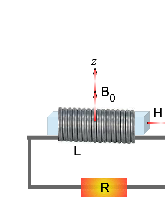
The overall setup is organized according to the scheme of Fig. 1, where the studied magnetic sample is inserted into a magnetic coil of an electric circuit playing the role of a resonator. The spin is in a metastable state, being frozen due to the low temperature and strong magnetic anisotropy. The moving spin of the sample creates electric current in the circuit that forms the feedback field acting on the sample. The feedback field satisfies the equation
| (3) |
in which is the circuit attenuation, is the circuit natural frequency, is the resonator filling factor, and the electromotive force is created by the moving average spin
| (4) |
The equations of motion are written for the spin averages
| (5) |
Pair spin correlations are decoupled employing the generalized mean-field approximation [6]
| (6) |
where and which is exact for and asymptotically exact for .
Let us introduce the notations for the Zeeman frequency
| (7) |
and the anisotropy frequencies
| (8) |
The dimensionless anisotropy parameter is
| (9) |
The dimensionless regulated field is defined as
| (10) |
The coupling between the magnetic sample and the resonator is characterized by the coupling rate
| (11) |
Also, introduce the notation for the dimensionless feedback field
| (12) |
Then the equations of spin motion read as
| (13) |
where
| (14) |
plays the role of an effective rotation frequency.
In the dimensionless notation, the feedback-field equation becomes
| (15) |
Efficient interaction between the electric circuit and the magnetic sample occurs when there happens a resonance between the effective Zeeman frequency of the sample spins and the resonator natural frequency . However, because of the presence of the anisotropy term, such a resonance cannot occur, since the detuning
| (16) |
can be very large.
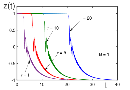
One of the possibilities for overcoming the above problem is to resort to the method of triggering resonance [18]. Assume that we need to overturn the spin at the moment of time . Then, tuning to , the regulated part of the magnetic field is kept zero before the time , and is switched on at the time , so that
| (19) |
At this initial moment of time , when the spin polarization is , the effective detuning becomes small,
| (20) |
which triggers the fast motion of spin reversal. Although the overall reversal is rather fast, but there appear tails, as is seen in Fig. 2.
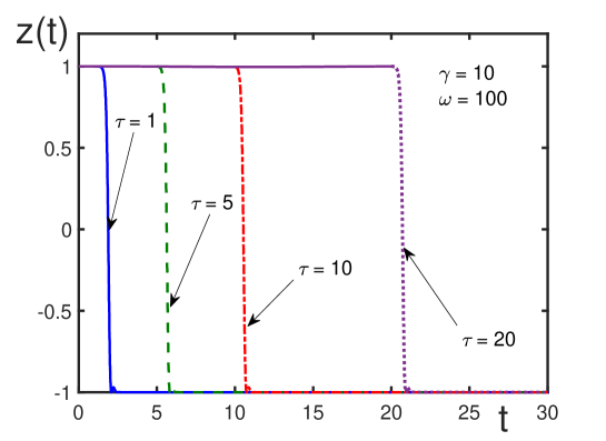
To preserve the resonance condition for the whole time of spin reversal, the method of dynamic resonance tuning is suggested [19]. Then the regulated field is varied so that to compensate the temporal variation of the anisotropy term . That is, the regulated field is switched on so that
| (23) |
which makes the effective detuning close to zero,
| (24) |
when . This method provides ideal conditions for keeping the spin frozen before the required time and then, at time , reversing the spin, as shown in Fig. 3.
3 Assemblies of nanomolecules or nanoclusters
It is possible to consider assemblies of nanomolecules or nanoclusters, when the system Hamiltonian has the form
| (25) |
where the first term is the Zeeman energy, the second term is the anisotropy energy
| (26) |
and, in addition, it is necessary to take account of the dipolar interactions through the dipolar tensor ,
| (27) |
The total magnetic field can be taken as
| (28) |
The anisotropy parameter usually is much smaller than , because of which one takes the anisotropy term as
| (29) |
The dynamics of the summary spin is similar to that of the spins of single nanosamples [5, 7, 8, 9, 10, 12, 15, 23, 24, 25, 27]. The role of the dipolar interactions is two-fold. First, the dipolar spin interactions trigger the initial spin motion by creating spin waves, and second, they result in the transverse spin attenuation leading to the dephasing of spin dynamics. The latter, however, does not strongly influence the coherent spin rotation, if the dephasing time is much longer than the reversal time. For nanomolecules and nanoclusters, the reversal time is of the order
| (30) |
4 Other magnetic nanomaterials
Except nanomolecules and nanoclusters, there are several other types of magnetic nanomaterials that can be employed for spintronic devices. Coherent spin motion in these materials can be regulated similarly to the case of nanomolecules and nanoclusters, considered above.
Emergence of defect-induced magnetism in graphene materials has been studied by Yazyev [28] and by Enoki and Ando [31]. Defects in graphene interact with each other through exchange interactions. The spin Hamiltonian consists of two terms, the Zeeman energy and the Heisenberg Hamiltonian,
| (31) |
The total magnetic field is the sum as in (28), including an external magnetic field and a feedback magnetic field. Peculiarities in the case of exchange interactions have been considered in detail in Ref. [48]. Dynamics of defect spins in graphene are considered in Refs. [32, 33]. Similar dynamics is exhibited by spins of quantum dots and some magnetic hybrid materials.
One more class of magnetic materials is presented by polarized nanomolecules that do not possess spins in their ground state, but nuclear spins inside them can be polarized by means of dynamic nuclear polarization [49, 50, 51]. This kind of molecules, for instance, are propanediol, butanol, and ammonia. Being spin polarized, they can keep this polarization for days and months. The Hamiltonian is
| (32) |
in which the term due to dipolar interactions is
| (33) |
where
The dipolar Hamiltonian (33) can be represented in the form (27), with the dipolar tensor
| (34) |
5 Trapped spinor atoms
Many atoms and molecules possessing dipolar or angular momenta can be confined in traps forming trapped clouds [34, 35, 36, 37, 38, 39, 40]. The derivation of an effective spin Hamiltonian for these objects goes in the following steps [39].
Let us assume that an atom has angular momentum
| (35) |
where , the quantum magnetic number takes the values . The field operators of atoms are the columns in the space of the magnetic number,
The Hamiltonian of a system composed of such atoms consists of several terms:
| (36) |
where
| (37) |
is a single-atom term without a magnetic field, the second part is a linear Zeeman term, the third part is a quadratic Zeeman term, the fourth part represents local atomic interactions, and the last part describes dipolar interactions. For the compactness of the formulas, here and in what follows, we set the Planck constant to one.
The linear Zeeman term is the standard expression
| (38) |
where is the atomic magnetic moment.
The quadratic Zeeman term consists of the sum
| (39) |
in which the first term in the write-had site describes static-current quadratic Zeeman effect and the second term, alternating-current quadratic Zeeman effect.
The nonresonant static-current quadratic Zeeman effect arises in atoms possessing hyperfine structure, hence a nonzero nuclear spin [54, 55, 56, 57, 58, 59]. The static-current quadratic Zeeman effect parameter reads as
| (40) |
where is a hyperfine energy splitting and is nuclear spin. The sign minus or plus in the static-current Zeeman parameter is defined by the relative alignment of the nuclear and the total electron spin projections of the atom: minus for parallel projections, while plus for antiparallel projections.
The quasi-resonant alternating-current quadratic Zeeman effect is due to the alternating-current Stark shift caused either by applying a linearly polarized microwave driving field inducing hyperfine transitions [60, 61, 62] or by applying off-resonance linearly polarized light inducing transitions between internal spin states [63, 64, 65, 66]. The alternating-current quadratic Zeeman effect parameter is
| (41) |
where is the Rabi frequency of the driving alternating field and is the detuning from an internal, spin or hyperfine, transition.
Local atomic interactions are presented by the Hamiltonian
| (42) |
in which is a matrix element of the interaction potential
| (43) |
where is the scattering length of a pair of atoms with the angular momentum of the pair and is a projection operator onto a state with an even angular momentum .
6 Insulating optical lattices
Trapped atoms can be loaded into deep optical latices, formed by laser beams, where the atoms become well localized and do not jump between lattice sites [67, 68, 69, 70]. Then the lattice is called insulating. For a periodic lattice, the field operators can be expanded over Wannier functions,
| (46) |
keeping in mind that at low temperature, the single-band approximation is valid. For an insulating lattice, the Wannier functions can be chosen to be well localized [71], so that the localization conditions be valid:
where is a smooth function of .
Let us introduce the local spin operator
| (47) |
satisfying the standard spin algebra for any statistics of , whether Bose or Fermi. The local density of atoms is defined as
| (48) |
The term (42) of local atomic interactions, for , becomes
| (51) |
with the parameters
| (52) |
in which and are the scattering lengths for collisions of atomic pairs.
7 Spin equations of motion
The spin equations of motion are obtained from the Heisenberg equations
| (58) |
It is straightforward to notice that
| (59) |
which is valid for any rotationally symmetric Hamiltonian with arbitrary . Therefore the spin motion is governed only by the spin part of the Hamiltonian,
| (60) |
with the spin Hamiltonian
| (61) |
Notice that the quadratic Zeeman Hamiltonian enters these equations, and its presence is important for governing spin dynamics [39, 40, 72, 73].
The spin equations of motion can be analyzed in several ways. First, it is possible to resort to quasiclassical approximation, when the spin operators are replaced by their averages and the resulting equations are solved numerically. This description is applicable at the coherent stage of spin motion, but it is not suitable for quantum stages of motion, especially at the initial stage of movement, where spin waves, triggering the spin motion, are necessary to initiate it.
The other method is based on the scale separation approach [45]. Then we write down the equations for the averages describing the transverse spin
| (62) |
coherence intensity
| (63) |
and longitudinal spin polarization
| (64) |
where are the ladder spin operators. The expressions describing local dipolar fluctuations, responsible for the creation of spin waves, are treated as stochastic variables [6, 39].
Keeping in mind the setup, discussed in Sec. 2, the spin equations of motion are complemented by the equation (3) for the feedback magnetic field or for its dimensionless form
| (65) |
with and being spin density.
To realize good resonance, the attenuations are to be small as compared to the Zeeman frequency
| (66) |
In that way, there are several small parameters in the system of equations:
| (67) |
where the spin-wave attenuation is
| (68) |
Spin fluctuations are proportional to , hence are also small.
In accordance to the small parameters (67), the variables and are classified as fast, while and , as slow. Following the scale separation approach, that is a variant of the Krylov-Bogolubov averaging technique [74], we solve the equations for fast variables and , with slow variables fixed. Then we substitute the found fast variables and into the equations for the slow variables and and average the right-hand sides of these equations for the slow variables over time and random fluctuations, with fixed slow variables and . As a result of this procedure, we obtain the guiding-center equations
| (69) |
where time is measured in units of . Here and are coupling functions
| (70) |
with the coupling parameter
| (71) |
and the notation
| (72) |
The quadratic Zeeman-effect parameter
| (73) |
is composed of the static-current quadratic Zeeman-effect parameter
| (74) |
and of the alternating-current quadratic Zeeman-effect parameter
| (75) |
The effective spin-rotation Zeeman frequency is
| (76) |
where the regulated field and the alternating-current quadratic Zeeman-effect parameter can be varied with time. It is therefore possible to regulate the detuning
| (77) |
so that either to make it large or negligibly small, respectively, either to freeze the spin or, by inducing the resonance, to organize a fast spin reversal, as is described in Sec. 2. The required resonance condition is
| (78) |
To estimate the typical order of the parameters, let us take the values for the atoms of 7Li, 21Na, 41K, and 87Rb. The spin density is cm-3, the attenuation rates are s-1, s-1, for a magnetic field G, we have s-1, .
The static-current parameter cm3, and . Also, , hence the contribution of the static-current effect into is .
In the case of the alternating current effect, s-1, then . Hence the contribution of the alternating-current effect into is . Thus, the parameter is mainly due to the static-current quadratic Zeeman effect.
8 Conclusion
The methods of regulating spin dynamics in different magnetic materials are studied. These materials include magnetic nanomolecules, magnetic nanoclusters, magnetic graphene, polarized nanomolecules, quantum dots, spinor atoms, and hybrid magnetic structures. The basic setup supposes the use of an electric circuit forming a feedback field acting on the magnetic sample and efficiently accelerating spin reversal. The ultrafast spin reversal can be realized in around s. The idea of employing a feedback field, in combination with the suggested method of triggering resonance, method of dynamic resonance tuning, and the use of the quadratic Zeeman effect can be applied in spintronics, e.g. for creating memory devices. Since there are many similarities between materials with magnetic moments and those possessing electric moments, the developed ideas and methods can be used for achieving fast reversal of electric dipoles. For instance, this can be employed for fast reversal of polarization in ferroelectrics coupled with electric cavity resonators [75, 76].
References
- [1] B. Barbara, L. Thomas, F. Lionti, I. Chiorescu, and A. Sulpice, Macroscopic quantum tunneling in molecular magnets, J. Magn. Magn. Mater. 200, 167 (1999).
- [2] A. Caneschi, D. Gatteschi, C. Sangregorio, R. Sessoli, L. Sorace, A. Cornia, M.A. Novak, C.W. Paulsen, and W. Wernsdorfer, The molecular approach to nanoscale magnetism, J. Magn. Magn. Mater. 200, 182 (1999).
- [3] V.I. Yukalov, Superradiant operation of spin masers, Laser Phys. 12, 1089 (2002).
- [4] V.I. Yukalov and E.P. Yukalova, Coherent nuclear radiation, Phys. Part. Nucl. 35, 348 (2004).
- [5] V.I. Yukalov and E.P. Yukalova, Coherent radiation by molecular magnets, Eur. Phys. Lett. 70, 306 (2005).
- [6] V.I. Yukalov, Nonlinear spin relaxation in strongly nonequilibrium magnets, Phys. Rev. B 71, 184432 (2005).
- [7] V.I. Yukalov, V.K. Henner, P.V. Kharebov, and E.P. Yukalova, Coherent spin radiation by magnetic nanomolecules and nanoclusters, Laser Phys. Lett. 5, 887 (2008).
- [8] V.I. Yukalov, V.K. Henner, and P.V. Kharebov, Coherent spin relaxation in molecular magnets, Phys. Rev. B 77, 134427 (2008).
- [9] V.K. Henner, V.I. Yukalov, P.V. Kharebov, and E.P. Yukalova, Collective spin dynamics in magnetic nanomaterials, J. Phys. Conf. Ser. 129, 012015 (2008).
- [10] V.K. Henner, P.V. Kharebov, and V.I. Yukalov, Superradiation from molecular nanomagnets, Solid State Phen. 152, 249 (2009).
- [11] J.R. Friedman and M.P. Sarachik, Single-molecule nanomagnets, Annu. Rev. Condens. Matter Phys. 1, 109 (2010).
- [12] V.I. Yukalov and E.P. Yukalova, Coherent spin dynamics of nanomolecules and magnetic nanoclusters, J. Phys. Conf. Ser. 393, 012004 (2012).
- [13] J.S. Miller, Organic and molecule-based magnets, Mater. Today 17, 224 (2014).
- [14] 7. G.A. Craig and M. Murrie, 3d single-ion magnets, Chem. Soc. Rev. 44, 2135 (2015).
- [15] V.I. Yukalov, V.K. Henner, and E.P. Yukalova, Spin superradiance by magnetic nanomolecules and nanoclusters, J. Phys. Conf. Ser. 594, 012006 (2015).
- [16] S.T. Liddle and J. van Slageren, Improving -element single molecule magnets, Chem. Soc. Rev. 44 6655 (2015).
- [17] B. Rana, A. K. Mondal, A. Bandyopadhyay, and A. Barman, Applications of nanomagnets as dynamical systems, Nanotechnology 33, 062007 (2021).
- [18] V.I. Yukalov and E.P. Yukalova, Triggering spin reversal in nanomolecules and nanoclusters on demand, Laser Phys. Lett. 19, 046001 (2022).
- [19] V.I. Yukalov and E.P. Yukalova, Method of dynamic resonance tuning in spintronics of nanosystems. Laser Phys. Lett. 19, 116001 (2022).
- [20] R.H. Kodama, Magnetic nanoparticles, J. Magn. Magn. Mater. 200, 359 (1999).
- [21] G.C. Hadjipanayis, Nanophase hard magnets, J. Magn. Magn. Mater. 200, 373 (1999).
- [22] W. Wernsdorfer, Classical and quantum magnetization reversal studied in nanometer-sized particles and clusters, Adv. Chem. Phys. 118, 99 (2001).
- [23] V.I. Yukalov and E.P. Yukalova, Possibility of superradiance by magnetic nanoclusters, Laser Phys. Lett. 8, 804 (2011).
- [24] V.I. Yukalov and E.P. Yukalova, Fast magnetization reversal of nanoclusters in resonator, J. Appl. Phys. 111, 023911 (2012).
- [25] P.V. Kharebov, V.K. Henner, and V.I. Yukalov, Optimal conditions for magnetization reversal of nanocluster assemblies with random properties. J. Appl. Phys. 113, 043902 (2013).
- [26] J. Kudr, Y. Haddad, L. Richtera, Z. Heger, M. Cernak, V. Adam, and O. Zitka, Magnetic nanoparticles: From design and synthesis to real world applications, Nanomaterials 7, 243 (2017).
- [27] V.I. Yukalov and E.P. Yukalova, Regulating spin dynamics in magnetic nanomaterials, Phys. Part. Nucl. Lett. 20, 1138 (2023).
- [28] O.V. Yaziev, Emergence of magnetism in graphene materials and nanostructures, Rep. Prog. Phys. 73, 056501 (2010).
- [29] H. Terrones, R. Lv, M. Terrones, and M. Dresselhaus, The role of defects and doping in 2D graphene sheets and 1D nanoribbons, Rep. Prog. Phys. 75, 062501 (2012).
- [30] E. Bekyarova, S. Sarkar, S. Niyogi, M.E. Itkis, and R.C. Haddon, Advances in the chemical modification of epitaxial graphene, J. Phys. D: Appl. Phys. 45, 154009 (2012).
- [31] T. Enoki and T. Ando, Physics and Chemistry of Graphene (Pan Stanford, Singapore, 2013).
- [32] V.I. Yukalov, V.K. Henner, and T.S. Belozerova, Generation of coherent radiation by magnetization reversal in graphene, Laser Phys. Lett. 13, 016001 (2016).
- [33] V.I. Yukalov, V.K. Henner, T.S. Belozerova, and E.P. Yukalova, Spintronics with magnetic nanomolecules and graphene flakes, J. Supercond. Nov. Magn. 29, 721 (2016).
- [34] A. Griesmaier, Generation of a dipolar Bose-Einstein condensate, J. Phys. B 40, R91 (2007).
- [35] M.A. Baranov, Theoretical progress in many-body physics with ultracold dipolar gases, Phys. Rep. 464, 71 (2008).
- [36] M.A. Baranov, M. Dalmonte, G. Pupillo, and P. Zoller, Condensed matter theory of dipolar quantum gases, Chem. Rev. 112, 5012 (2012).
- [37] D.M. Stamper-Kurn and M. Ueda, Spinor Bose gases: Symmetries, magnetism, and quantum dynamics, Rev. Mod. Phys. 85, 1191 (2013).
- [38] B. Gadway and B. Yan, Strongly interacting ultracold polar molecules, J. Phys. B 49, 152002 (2016).
- [39] V.I. Yukalov and E. P. Yukalova, Spin dynamics in lattices of spinor atoms with quadratic Zeeman effect, Eur. Phys. J. D 72, 190 (2018).
- [40] V.I. Yukalov, Dipolar and spinor bosonic systems, Laser Phys. 28, 053001 (2018).
- [41] D.A. Schwartz, N.S. Norberg, Q.P. Nguyen, J.M. Parker, and D.R. Gamelin, Magnetic quantum dots: Synthesis, spectroscopy, and magnetism of Co and NiDoped ZnO Nanocrystals, J. Am. Chem. Soc. 125, 13205 (2003).
- [42] J.L. Birman, R.G. Nazmitdinov, and V.I. Yukalov, Effects of symmetry breaking in finite quantum systems, Phys. Rep. 526, 1 (2013).
- [43] K.D. Mahajan, Q. Fan, J. Dorcena, G. Ruan, and J.O. Winter, Magnetic quantum dots in biotechnology–synthesis and applications, Biotechnol. J. 8, 1424 (2013).
- [44] A. Tufani, A. Qureshi, and J.H. Niazi, Iron oxide nanoparticles based magnetic luminescent quantum dots (MQDs) synthesis and biomedical/biological applications: A review, Mater. Sci. Eng. C 118, 111545 (2021).
- [45] V.I. Yukalov and E.P. Yukalova, Cooperative electromagnetic effects Phys. Part. Nucl. 31, 561 (2000).
- [46] V.I. Yukalov and E.P. Yukalova, Coherent nuclear radiation, Phys. Part. Nucl. 35, 348 (2004).
- [47] S. Odenbach, Magnetic hybrid materials, Arch. Appl. Mech. 89, 1 (2019).
- [48] V.I. Yukalov and E.P. Yukalova, Coherent radiation by magnets with exchange interactions, Laser Phys. 25, 085801 (2015).
- [49] V.I. Yukalov, Coherent radiation from polarized matter, Laser Phys. 3, 870 (1993).
- [50] V.I. Yukalov, Transient coherent phenomena in radiofrequency region, Laser Phys. 5, 526 (1995).
- [51] V.I. Yukalov, Theory of coherent radiation by spin maser, Laser Phys. 5, 970 (1995).
- [52] V.I. Yukalov, M.G. Cottam, and M.R. Singh, Nonlinear dynamics of nuclear-electronic spin processes in ferromagnets, J. Appl. Phys. 85, 5627 (1999).
- [53] V.I. Yukalov, M.G. Cottam, and M.R. Singh, Nonlinear spin dynamics in ferromagnets with electron-nuclear coupling, Phys. Rev. B 60, 1227 (1999).
- [54] F.A. Jenkins and E. Segre, The quadratic Zeeman effect, Phys. Rev. 59, 52 (1939).
- [55] L.I. Schiff and H. Snyder, Theory of the quadratic Zeeman effect, Phys. Rev. 59, 59 (1939).
- [56] J. Killingbeck, The quadratic Zeeman effect, J. Phys. B 12, 25 (1979).
- [57] S.L. Coffey, A. Deprit, B. Miller, and C.A. Williams, The quadratic Zeeman effect in moderately strong magnetic fields, Ann. New York Acad. Sci. 497, 22 (1987).
- [58] G.K. Woodgate, Elementary Atomic Structure, Oxford University, Oxford, 1999.
- [59] W. Demtröder, Molecular Physics, Wiley, Berlin, 2005.
- [60] F. Gerbier, A. Widera, S. Folling, O. Mandel, and I. Bloch, Resonant control of spin dynamics in ultracold quantum gases by microwave dressing, Phys. Rev. A 73, 041602 (2006).
- [61] S.R. Leslie, J. Guzman, M. Vengalattore, J.D. Sau, M.L. Cohen, and D.M. Stamper-Kurn, Amplification of fluctuations in a spinor Bose-Einstein condensate, Phys. Rev. A 79, 043631 (2009).
- [62] E.M. Bookjans, A. Vinit, and C. Raman, Quantum phase transition in an antiferromagnetic spinor Bose-Einstein condensate, Phys. Rev. Lett. 107, 195306 (2011).
- [63] C. Cohen-Tannoudji and J. Dupon-Roc, Experimental study of Zeeman light shifts in weak magnetic fields, Phys. Rev. A 5, 968 (1972).
- [64] L. Santos, M. Fattori, J. Stuhler, and T. Pfau, Spinor condensates with a laser-induced quadratic Zeeman effect, Phys. Rev. A 75, 053606 (2007).
- [65] K. Jensen, V.M. Acosta, J.M. Higbie, M.P. Ledbetter, S.M. Rochester, and D. Budker, Cancellation of nonlinear Zeeman shifts with light shifts, Phys. Rev. A 79, 023406 (2009).
- [66] A. de Paz, A. Sharma, A. Chotia, E. Marechal, J. Huckans, P. Pedri, L. Santos, O. Gorceix, L. Vernac, and B. Laburthe-Tolra, Nonequilibrium quantum magnetism in a dipolar lattice gas, Phys. Rev. Lett. 111, 185305 (2013).
- [67] O. Morsch and M. Oberthaler, Dynamics of Bose-Einstein condensates in optical lattices, Rev. Mod. Phys. 78, 179 (2006).
- [68] C. Moseley, O. Fialko, and K. Ziegler, Interacting bosons in an optical lattice, Ann. Phys. (Berlin) 17, 561 (2008).
- [69] V.I. Yukalov, Cold bosons in optical lattices, Laser Phys. 19, 1 (2009).
- [70] K.V. Krutitsky, Ultracold bosons with short-range interaction in regular optical lattices, Phys. Rep. 607, 1 (2016).
- [71] N. Marzari, A.A. Mostofi, J.R. Yates, I. Souza, and D. Vanderbilt, Maximally localized Wannier functions: Theory and applications, Rev. Mod. Phys. 84, 1419 (2012).
- [72] V.I. Yukalov and E.P. Yukalova, Influence of quadratic Zeeman effect on spin waves in dipolar lattices, J. Magn. Magn. Mater. 465, 450 (2018).
- [73] V.I. Yukalov and E.P. Yukalova, Regulating spin reversal in dipolar systems by the quadratic Zeeman effect, Phys. Rev. B 98, 144438 (2018).
- [74] N.N. Bogolubov and Y.A. Mitropolsky, Asymptotic Methods in the Theory of Nonlinear Oscillations Gordon and Breach, New York, 1961.
- [75] V.I. Yukalov and E.P. Yukalova, Ultrafast polarization switching in ferroelectrics Phys. Rev. Res. 1, 033136 (2019).
- [76] V.I. Yukalov, Superradiance by ferroelectrics in cavity resonators, Laser Phys. 29, 124007 (2019).