revtex4-1Repair the float
Interacting Mathieu equation, synchronization dynamics and collision-induced velocity exchange in trapped ions
Abstract
Recently, large-scale trapped ion systems have been realized in experiments for quantum simulation and quantum computation. They are the simplest systems for dynamical stability and parametric resonance. In this model, the Mathieu equation plays the most fundamental role for us to understand the stability and instability of a single ion. In this work, we investigate the dynamics of trapped ions with the Coulomb interaction based on the Hamiltonian equation. We show that the many-body interaction will not influence the phase diagram for instability. Then, the dynamics of this model in the large damping limit will also be analytically calculated using few trapped ions. Furthermore, we find that in the presence of modulation, synchronization dynamics can be observed, showing an exchange of velocities between distant ions on the left side and on the right side of the trap. These dynamics resemble to that of the exchange of velocities in Newton’s cradle for the collision of balls at the same time. These dynamics are independent of their initial conditions and the number of ions. As a unique feature of the interacting Mathieu equation, we hope this behavior, which leads to a quasi-periodic solution, can be measured in current experimental systems. Finally, we have also discussed the effect of anharmonic trapping potential, showing the desynchronization during the collision process. It is hopped that the dynamics in this many-body Mathieu equation with damping may find applications in quantum simulations. This model may also find interesting applications in dynamics systems as a pure mathematical problem, which may be beyond the results in the Floquet theorem.
I Introduction
Mathieu’s equation, which holds a prominent place in mathematical physics, has a fascinating historical origin dating back to the 19th century. Emile Mathieu conducted research on the vibrations of elliptical drums. His work was motivated by the broader scientific context of understanding the wave phenomena, particularly in the study of acoustics and vibrations. In 1868, Mathieu published his seminal work and his investigations are rooted in the Helmholtz equation Ruby (1996); Bibby and Peterson (2013)
| (1) |
in which the solutions are defined as . In the elliptic cylinder coordinates , , and . In the above equation, the curve by gives the confocal ellipses and the curve by gives the orthogonal hyperbolas. If we define and , or and , then we will obtain the same ordinary differential equation, now known as the Mathieu equation, which emerged as a solution to describe the complex oscillatory patterns observed in elliptical hoops Mathieu (1868). For this reason, the Mathieu and the modified Mathieu equation can emerge from any differential equations involving the Helmholtz equations expressed in the elliptic cylinder coordinates. It has been discussed in details by Paul in 1953 - 1958; see Ref. Paul (1990) and references therein. For a long time, the Mathieu equation has been one of the most important linear differential equations studied in mathematics and physics Landau and Lifshitz (1976); Bhattacharjee et al. (2007), and can be written as the following second-order linear ordinary differential equation Richards (1983); Paul (1990)
| (2) |
Here is the time, is the vibration amplitude, and the coefficients and known as the Mathieu parameters, completely determine the stability of the dynamics. Obviously, the differential operator itself is a periodic function, with period , however the solution is not necessarily periodic, but instead, a quasi-periodic solution is allowed. This kind of quasi-periodicity is a typical feature of differential equations in dynamical systems 111For example, let us consider the following ordinary differential equation , with solution , which is not a periodic solution of . However, it is a quasi-periodic solution satisfying , as expected from the Floquet theorem. .
The above Mathieu equation is a special condition of the Hill equation, which can be written as
| (3) |
where are constants. The solution is related to a determinant of an infinite matrix. When only and are involved and for all , it will be reduced to the Whittaker-Hill equation Parra-Verde and Gutiérrez-Vega (2024); Urwin and Arscott (1970); Koenig (1933).
In Ref. Ruby (1996), a lot of important applications have been summarized, including elliptic drums, inverted pendulum, radio frequency quadrupole, modulated LC circuit, floating body etc... In recent years, some major attention have been payed to the Paul trap for charged particles and mirror trap for neutral particles. In Refs. Daniel (2020); Sinclair (2014); Cirac and Zoller (2000); Steven Ban and Wen (2016), applications of the Mathieu equation in wave propagation in pips, electromagnetic wave guides and oscillations of water in a lake have also been presented. In these applications, the physics in the Paul trap is the major concern in this work for its potential applications in quantum computation, following the scheme by Cirac and Zoller Cirac and P. (1995).
The Mathieu model provides a mathematical framework to understand the behavior of charged particles in various types of traps. Trapped ions are confined spatially by electric or magnetic fields, and their motion within these traps is described by the Mathieu equation Leibfried et al. (2003); Paul (1990). In this case, the dynamics are fully determined by several parameters: , and the damping rate (see below). Moreover, the trap geometry and field strength are also determined from the values of these parameters Savaryn et al. (2016); Paul (1990); Thompson et al. (2002). Motivated by these researches, in this work, we extended the single particle Mathieu equation to the many-body Mathieu equation, and study its dynamics based on classical equations. This work is organized in the following way. The dynamics in the quantum regime need to be considered elsewhere. We first start by presenting the criterion for stability and instability based on Floquet theorem in Sec. II. Then, in Sec. III, we study the dynamics with two to four trapped ions, in which in the large damping limit, the dynamics can be solved analytically. In this case, we show how the damping rate influences the relative phase and the vibration amplitude around their equilibrium positions. In Sec. IV, we study the dynamics with trapped ions with a finite damping rate. In Sec. V, we examine the stability and the phase chart in the many-body Mathieu equation, which has been argued in the previous section. We show that the phase chart is independent of the many-body interaction. In Sec. VI, the fate of the phase chart and the stability is examined in the presence of anharmonic nonlinear potential, showing that the parametric resonance is absent in the presence of a cubic nonlinear coefficient. Finally, we discuss the experimental relevance of our results in Sec. VII. We conclude this work and discuss the unique feature of this many-body Mathieu model and its potential applications in Sec. VIII.
II Stability of the Mathieu equation and the phase chart
The Mathieu equation is the simplest equation to study the stability and instability of a system with a periodic driving force, which is known as parametric resonance. This behavior is totally different from the forced resonance in the linear differential equation. In the forced resonance, the resonance can only happen when the driving frequency is the same as the intrinsic vibrational frequency of the system, in which the vibrational amplitude increases linearly with time . However, in the parametric resonance, the resonance can be found in a wide range of parameters, with a vibrational amplitude increasing exponentially with time Landau and Lifshitz (1976); Bhattacharjee et al. (2007); Wu and Diebold (2012). In the following, we discuss the phase chart of the Mathieu equation with and without damping Trypogeorgos and Foot (2016).

We can use the Floquet theory to understand the stability of this model. Let us consider the following equation with periodic coefficients Kovacic et al. (2018); Stafford et al. (1984); Richards (1976)
| (4) |
where is the damping rate Acar and Feeny (2016); Turyn (1993). This equation can be defined as Sinha and David (2001)
| (5) |
We will obtain two independent solutions, that can be denoted as , and , with the initial conditions
| (6) |
Furthermore, we can construct the solutions as
| (7) |
with , which based on the Floquet theory, its solution should be . One can check this solution . Using the initial condition that , we can immediately obtain
| (8) |
In this way, we expect . Thus, the system is stable when and only when the eigenvalues of , which are assumed by , satisfy . We can obtain the eigenvalues of the matrix using
| (9) |
The above equation is used to determine the phase boundary. In the above solution, we have and , thus is a real matrix; yet non-Hermite. (I) When the solution is real, we should have a phase boundary at ; (II) When is a complex, the two solutions are complex valued, and we expect . The second condition will corresponds to the condition without damping Wilkinson et al. (2018); Jia et al. (2016).
The phase boundary is fully determined by the two parameters and . We find that the phase boundaries are determined by the regime enclosed by the following condition
| (10) |
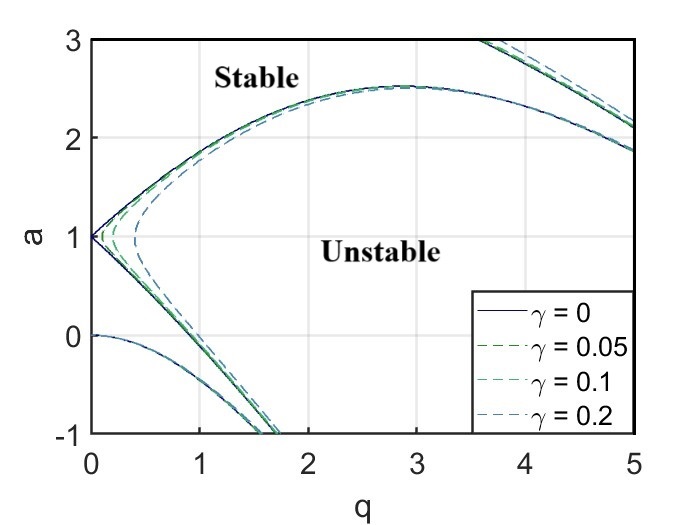
With this theory, we can determine the phase boundary as a function of and . In Fig. 1, we present the phase chart without damping Koad et al. (2023); Nop et al. (2023), and in Fig. 2, we present the results with damping Rand (2012); Insperger and Stepan (2003). The roots of the equation without damping are given by
| (11) |
and the stable phase is given by Taylor and Narendra (1969); Konenkov et al. (2002). In this condition, is a complex number, and we can prove exactly that , in this condition we can define .
We see that the damping has the effect of reducing the unstable regions of the system, which is consistent with our intuition; see Kovacic et al. (2018); Poulin and Flierl (2008) and Ref. Landau and Lifshitz (1976). Whenever there is a dissipation of energy, the system goes to rest, which naturally means that it becomes stable. However, in the following section, we will present a different role played by the dissipative term on the relation between the vibration amplitude and the equilibrium position in the strong damping limit.
III Dimensionless and large damping limits
Now, we turn to the major results that will be presented in this work. Our aim is to study the dynamics of trapped ions in the presence of a strong Coulomb interaction. The Hamiltonian for trapped ions can be written as
| (12) |
where
| (13) | |||
| (14) |
In the above model, is the mass of the trapped ions, is the vacuum permittivity, is the modulation frequency, and is the system’s frequency. The equation of motion of this model can then be written as
| (15) | |||||
Here is introduced for the damping effect.
Now, we use the following transformation to make the equation dimensionless
| (16) |
Substituting the new variables and parameters into the original equation results in the following interacting Mathieu equation
| (17) |
Hereafter, we have defined a differential operator as
| (18) |
Now all the quantities became dimensionless, and their values are of the order of unity. In the last term, the minus sign represents the repulsive interaction between the charged ions. Obviously, when and is very small, the trapping potential may become unbounded from below, which may lead to instability.
III.1 The case of two ions
The dynamics of a system of two ions can be effectively analyzed through the decomposition of the system into two components: the motion of the center of mass and the motion of the relative position of the ions. This decomposition simplifies the analysis by reducing the problem from a complex two-body interaction to two independent single-body equations. To this end, we define , and . The system yields two equations
| (19) |
These two equations lead to two independent equations as following
| (20) |
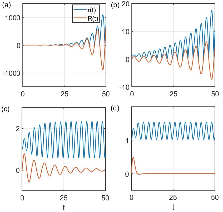
Here the first equation (the motion of the relative position) corresponds to the damped Mathieu equation, and the second one (the motion of the center of mass) corresponds to the same damped Mathieu equation but with a Coulomb interaction term. In the instability phase when , the center of mass will be reduced to the linear Mathieu equation. For this reason, these two equations have the same phase boundary for stability-instability transitions. However, in the stable phase, their dynamics will be totally different. We find that is the solution of the center of mass, but is not the solution of the relative position. For this reason, even in the presence of damping, the motion of the relative position will always oscillate in some way. Moreover, due to the non-penetration effect of the trapped ions, the motion of will be restricted to or , depending on its initial value. The results for various damping rates are presented in Fig. 3, showing that in the stable phase when , will always oscillate periodically around its equilibrium position with the same period of the Mathieu equation.
In the case of strong damping (see Fig. 3 (d)), we may assume , where is the equilibrium position, one may find that oscillates in the way of the driving dynamics. When , we expect , yielding for used in Fig. 3. Thus, we assume that the dynamics are the following
| (21) |
where is a phase introduced by the damping effect. Inserting this solution into the above equation, and to the leading term, we get
| (22) | |||||
| (23) |
These two terms correspond to the coefficients of and , which should be equal to zero. The higher-order terms such as and are neglected. The solutions of and can be written as
| (24) |
and
| (25) |
In the large limit, we expect , or . In this limit, we expect the solution to be
| (26) |
This solution can be understood by assuming , where for small and , we have
| (27) |
For the four terms between the brackets, the term dominates and we have
| (28) |
yielding the following solution
| (29) |
in Eq. 26. For this reason, the effect of damping influences the vibration amplitude, instead of driving the ions to rest. This picture applies to the conditions of more trapped ions.
The above results can also be understood from the balance between the energy introduced by the driving force and the energy dissipated by the damping force. We have
| (30) | |||||
| (31) |
A direct calculation using will yield the above relation, with (see Eq. 29)
| (32) |
This method has been used in Ref. Landau and Lifshitz (1976) in the determination of the vibration amplitude of the damped oscillator, and the same idea can be used to understand the vibration amplitude in our model. As a result, when the vibration amplitude will increase due to the absorption of the energy from the driving field; otherwise, it will decrease. This picture can be used to understand the quasi-periodic motion of the trapped ions, as discussed below. Thus, the quasi-periodic solution can also be found in nonlinear driven equations.
III.2 The case of three ions
The same method can be applied to three trapped ions, by defining , , and . This results in a system of three coupled equations
| (33) | |||
| (34) | |||
| (35) |
With this definition, we can obtain the equation of the center of mass as , which is exactly the same as the driving Mathieu equation. This conclusion can be extended to arbitrary ions. The equations of motion for and can be written as
| (36) | |||||
| (37) |
We first start by defining the equilibrium position equations for a strong damping , and . In the large limit, we neglect , and would obtain
| (38) |
Therefore, the solutions would be
| (39) |
Using the perturbation theory, and assuming to be small, we obtain from its equation of motion that
| (40) | |||||
| (41) |
The solutions of and can be written as
| (42) |
In the large limit, , expecting the solution to be
| (43) |
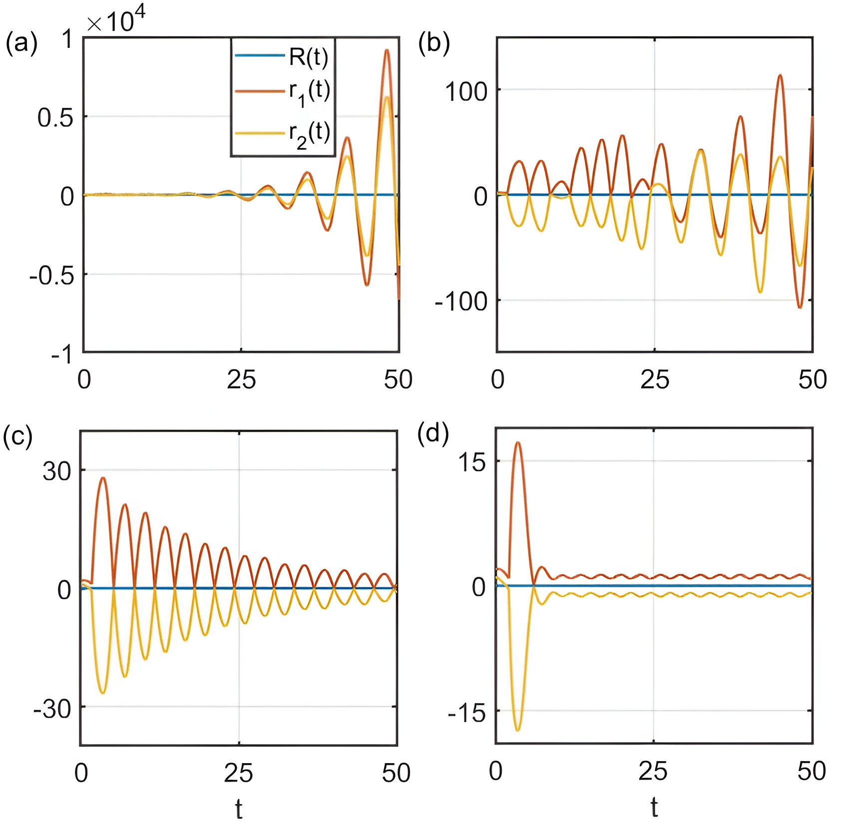
Obviously, the vibration amplitude in this solution also satisfies the energy balance condition of Eq. 32. This solution has been verified using numerical data. In Fig. 4, we present the results for three trapped ions, showing that in the large limit, indeed, when , and will vibrate around their equilibrium positions, which can be well described by the above analytical solution
| (44) |
which yields ; see Eq. 43.
III.3 The case of four ions
This method can be extended to any arbitrary number of trapped ions, and here we will only present results for . In a similar way, for and we can define
| (45) |
This result is based on numerical simulation, showing that in the large limit, the trapped ions 1 and 4 (and 2 and 3) can have almost opposite dynamics. From the equation of motion and assuming to be small in comparison to , we obtain
| (46) |
which can not be solved analytically. We also find using numerical fitting that
| (47) |
which can be understood using Eq. 32. From these results, we expect that in the condition of , we should have and , up to some universal constants to be determined numerically.
So far, we focused on studying systems in the strong damping limit, and what we noticed is that it have barely any influence on the total energy of the ions. This means that despite the presence of damping from the environment or the laser field, the total energy of the system remains relatively conserved. The damping does not extract a significant large energy from the system, that is why it remains stable over time; see discussion in the next section. As a result, in this regime, the strong damping only influences the oscillation amplitudes of the ions around their equilibrium positions. In the following, we will only focus on the dynamics with finite damping, which will yield some new interesting features.
III.4 Anharmonic effect
The above analysis — based on the center of mass and the relative coordinates — depends strongly on the linearity of the equation of motion. In the presence of anharmonic effects in the trapping potential, the calculation is much more complicated. It has some profound impact on the dynamics of the system. Firstly, the method of the center of mass and the relative positions can not be applied anymore; and secondly, the phase chart and stability can be changed even in the nonlinear Mathieu equation; and thirdly, the criterion for stability based on the Floquet theorem will no longer be valid. For these reasons, the quasi-periodic solution may not be observed.
To this end, let us consider the following model with with strong damping. The equation of motion can be written as
| (48) |
Let us assume that , and , where by symmetry the equilibrium position of the first and third ions should be at and the equilibrium position of the second ion should be at zero. This solution is supported by numerical evidences in Fig. 5. In the case of strong damping , , thus we have
| (49) |
This equation is the same as Eq. 38 when , and will be solved using numerical methods. Using perturbation theory again, we will find the leading terms of the equations (with )
| (50) |
for the coefficient of , allowing us to obtain the expressions of
| (51) |
The coefficient of is neglected. A much better approximation of the solutions is using Eq. 39, with a finite relative phase. These solutions are the same as Eq. 32. The equilibrium position can be numerically determined using Eq. 49. Obviously, with the increasing of (assuming ), will decrease monotonically. In the large limit, we should have .
We see that in the condition of anharmonic effects in the trapping potential, we still have the relation in Eq. 32 for the balance between the driving force and the damping force averaged in one full period. Therefore, the anharmonic effects, , in the trapping potential only influences the vibration amplitude in a way of Eq. 49. A simple and straightforward argument will show that this conclusion to be correct even with many trapped ions.
IV Exchange of velocities and Newton’s cradle
IV.1 Without damping
Then, what will happen in the presence of finite damping? Generally speaking, the dynamics and vibration amplitudes depend on the competition of the driving forces, which may introduce some energy to the system, and the damping force, which can extract energy from the system. In the large limit, these two forces are balanced, leading to periodic vibrations. In the long time limit, we find that the dynamics of the trapped ions are independent of their initial positions and velocities (see Eq. 45). In the weak damping limit, the physics will be totally changed. For example, in the model without damping, this system should support a quasi-periodic solution, instead of a periodic solution, and large vibrations of the amplitude of the ions will be possible, in which the distance between the ions may become very small, leading to large forces from the repulsive Coulomb interaction. In this way, the dynamics will exhibit some new features, which resembles to the dynamics of Newton’s cradle; see Fig. 7. This motivate our following investigations.
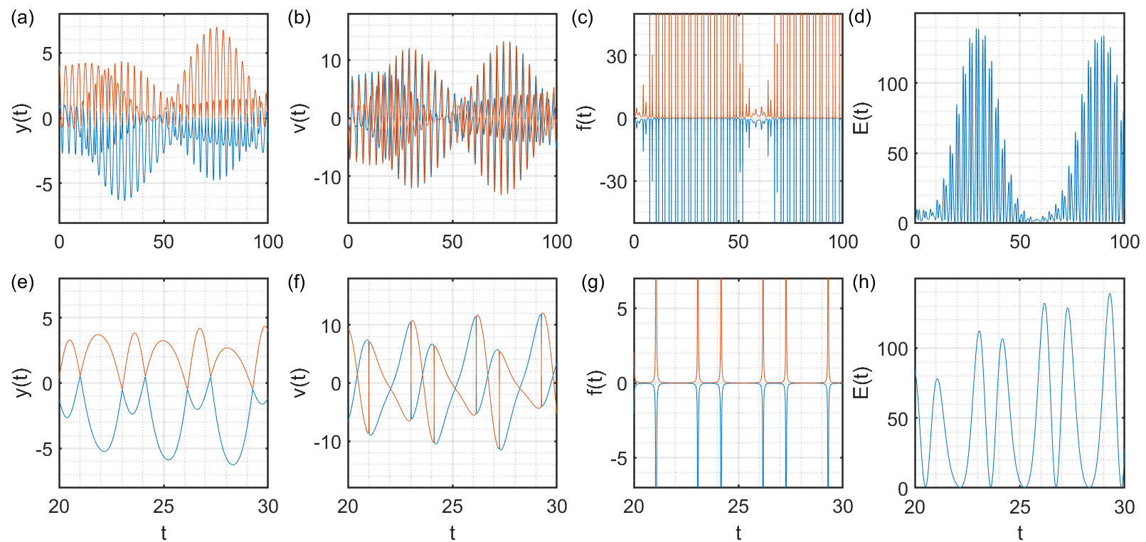
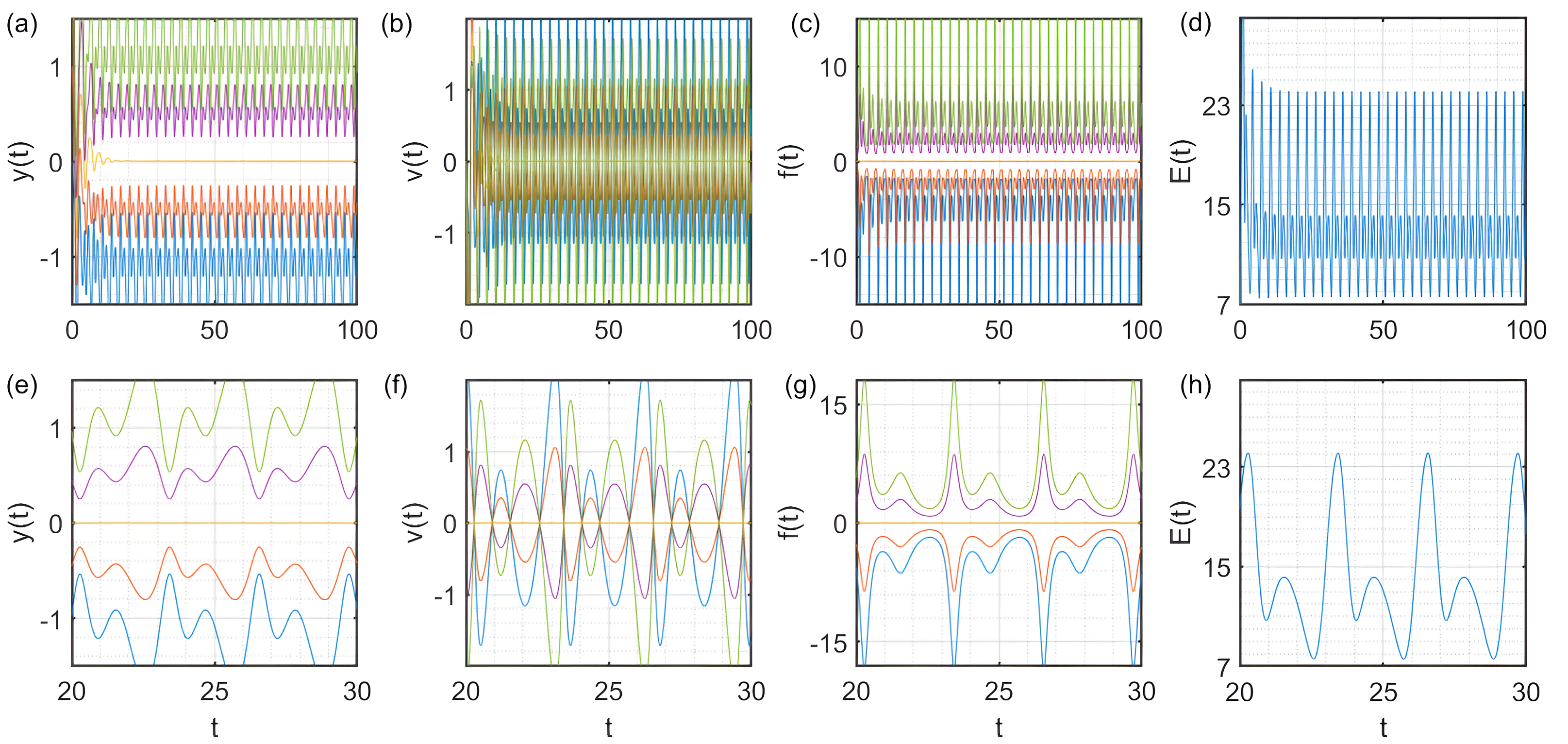
We will focus on the following quantities: the positions , the velocities , the forces , and the energy . Here, is the total energy of the system defined by the kinetic energy, the trapping energy and the Coulomb energy. When two ions approach each other, the force may diverge, leading to dramatic changes of velocities — exchange of velocities — van Mourik et al. (2022), which is the same as the dynamics in Newton’s cradle. Furthermore, when the total energy increases, the system absorbs energy from the driving force; otherwise, the driving force will extract energy from the system.
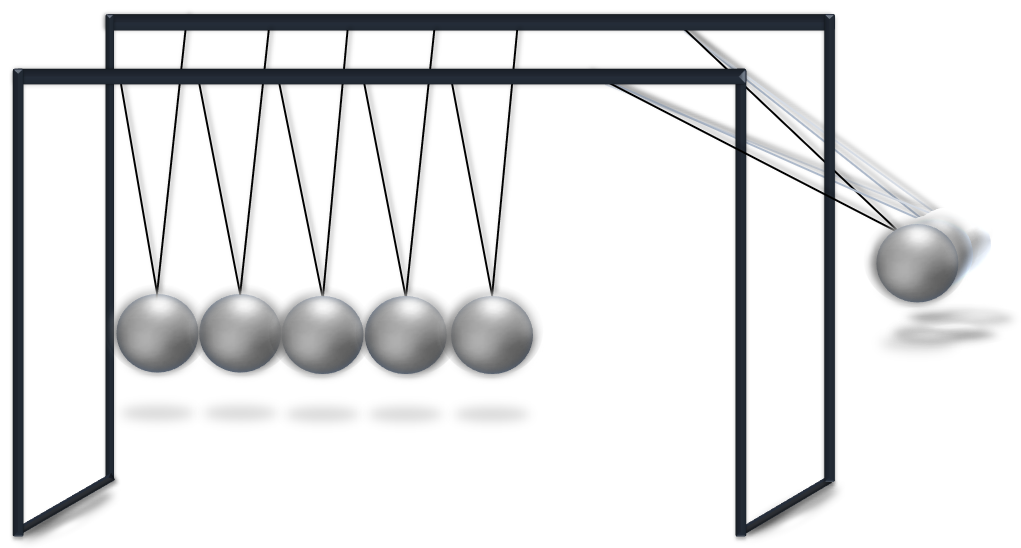

The results for , , and for two trapped ions are presented in Fig. 6 without damping. We focus on the stable regime. The dynamics of and exhibit some interesting features not presented in the strong damping limit. Firstly, it presents some kind of micromotion with period from the driving field; and secondly, the system shows some global structure with much larger period, not necessary to the commensurate with the period of the driving field. In this way, the system displays some quasi-periodic dynamics. The velocity also exhibits similar dynamics in Fig. 6 (b). We find that the vibration amplitude and the velocity are greatly enhanced, indicating that the system continuously absorbing and releasing energy from the driving field. In Fig. 6 (f), we plot the detailed dynamics of the velocity, showing that when two ions are approaching each other (see Fig. 6 (e)), there is a sudden exchange of velocities, which is the same as that in Newton’s cradle (Fig. 7). Our model may be the smallest system for the realization of Newton’s cradle. At this point, the force will become divergent or significantly large; see Fig. 6 (c) and (g). In Fig. 6 (d), we calculate the total energy of this model, showing that the total energy has the same quasi-periodic structure for the motion and the velocity. These results represent some unique features of the interacting Mathieu equation with the many-body Coulomb force.
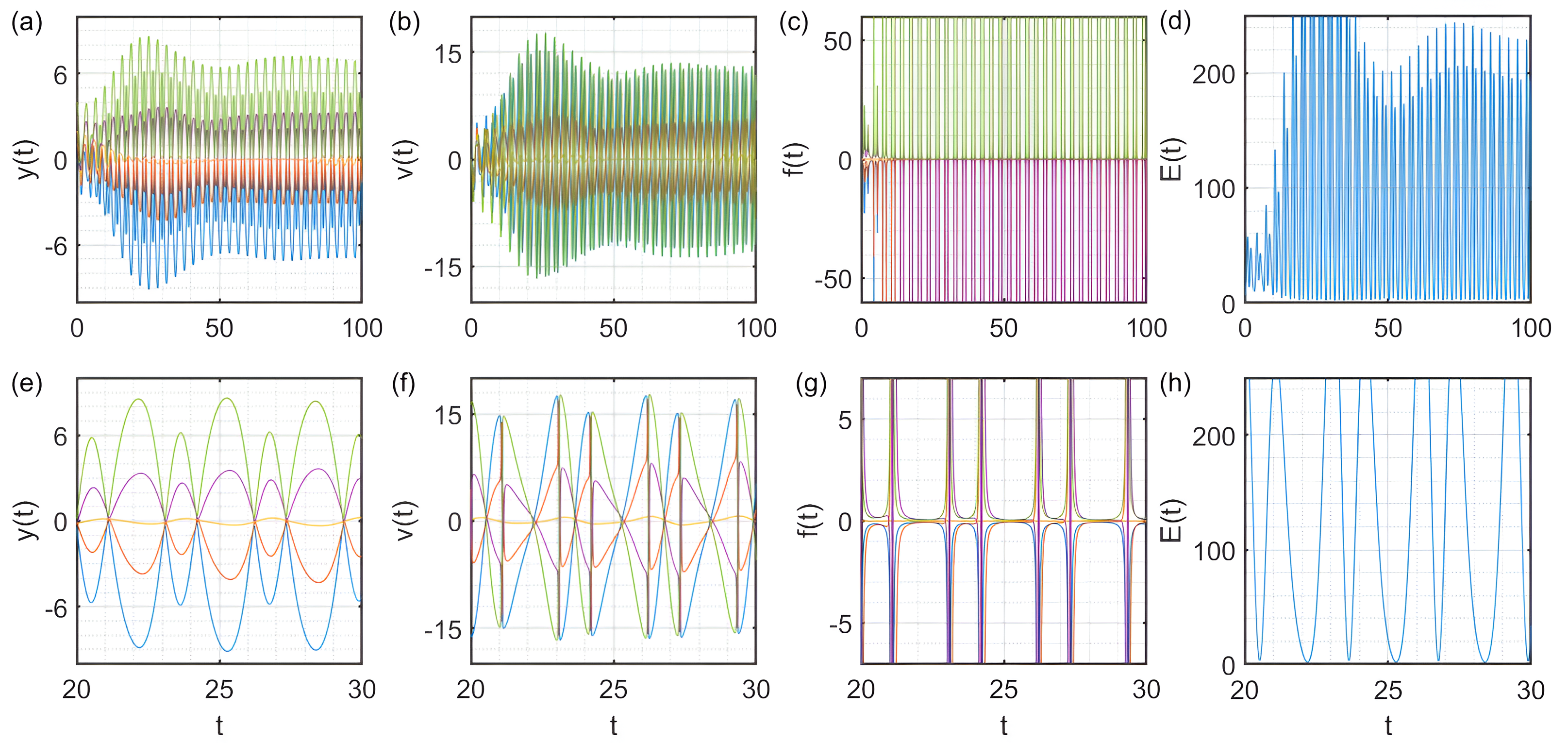
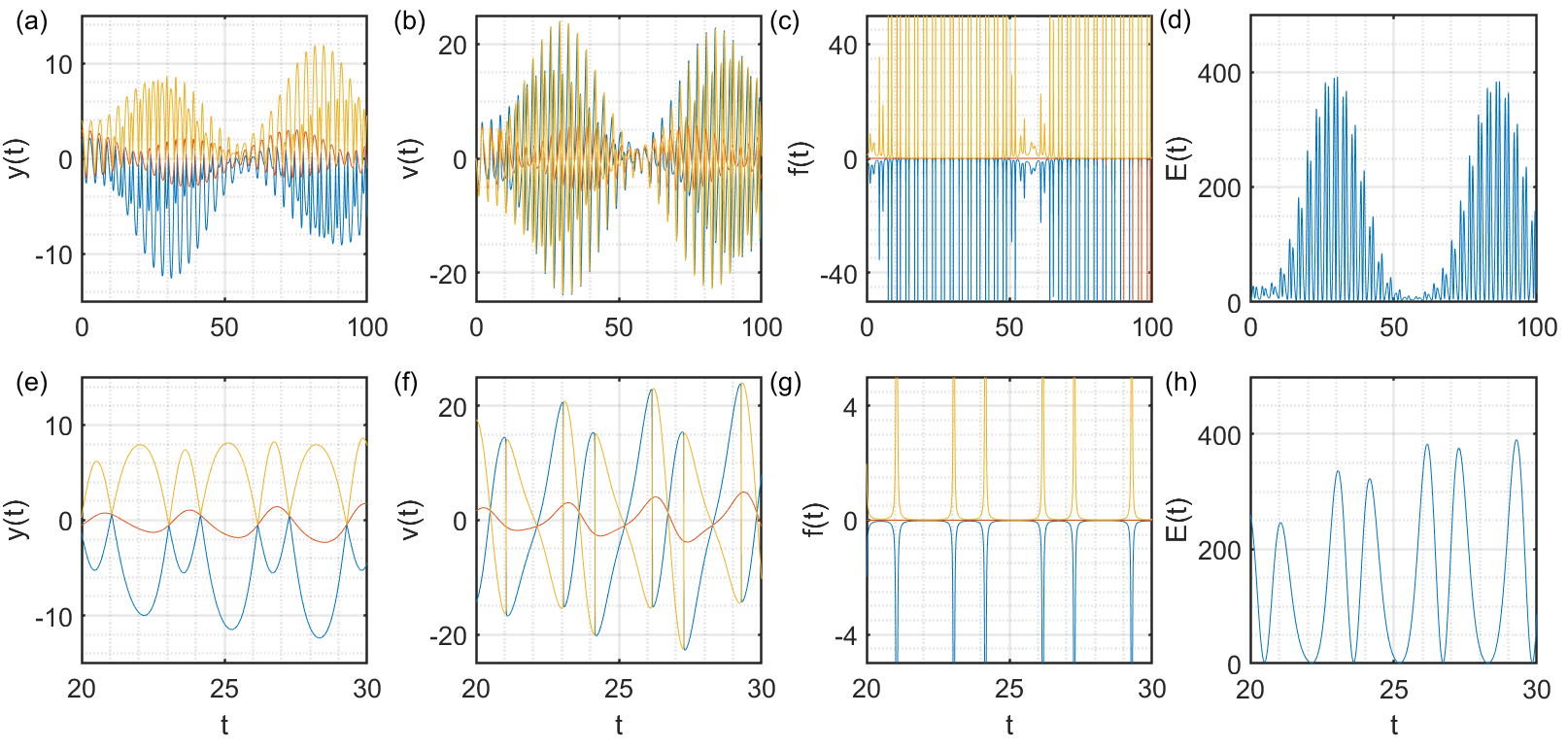
Next, we are in a position to understand what will happen in the presence of many trapped ions. In Newton’s cradle, the exchange of velocities happens between two colliding balls; and the more number of balls involved the more complicated the dynamics become. To this end, we present the results for three trapped ions in Fig. 8 and for five trapped ions in Fig. 9 without damping. In these two figures, we always find the sudden exchange of velocities when all the ions are colliding with each other. The most striking feature is that in the presence of many trapped ions (), the motion of the ions will be synchronized in such a way that they will collide to each other almost at the same time. We have verified that similar features can be found for much larger systems (for example, ), and these synchronization dynamics are independent of their initial positions and initial velocities. As a result, for three trapped ions, the exchange of velocities happens between and (assuming ); and for five trapped ions, the exchange of velocities happen between and , and and . The synchronization dynamics are a unique feature in our model.
These results should not be mixed up with the melting of ions, in which the structure is totally destroyed van Mourik et al. (2022). In this case, the distance between the ions will increase, leading to the destruction of the crystal structures. In our model, we indeed found the dramatic increase of the distance between the ions, however, these ions are still trapped in the potential, and their distances will be decreased after some proper time, leading to coherent quasi-periodic dynamics. In this way, the structure of the ions will not be destroyed.
IV.2 Effect of damping
With the above dynamics, we need to understand the role of the damping in the many-body Mathieu equation, in which we expect a transition from the undamped physics discussed in the above subsection to the strong damping physics discussed in the large limit. These physics are intriguing not only because of the effect of damping on the exchange of velocities, but also from the transition from a quasi-periodic solution to a periodic vibrational solution.
By focusing on the dynamics of a system of five ions, we can observe much more the ion-ion interactions and highlight the unique features of damping. In the stable regime, the results for , , and for five trapped ions with a weak damping and a strong one are presented in Fig. 10 and Fig. 11, respectively. In the case of weak damping, the system behaves almost exactly the same as without damping. This is seen in Fig. 10 (a) and (e), the ions oscillate in a quasi-periodic way where they approach each other, the Coulomb force becomes strong in Fig. 10 (c) and (g), leading to a sudden exchange of velocities , as observed before. In this condition, each ion will mirror the furthest ion in the system, thus we observe that ion exchanges its velocity with ion , and exchanges its velocity with ion , leaving ion to be almost unchanged. This is a unique feature from Newton’s cradle, in which the kinetic energy is transferred from the left furthest ball to the right furthest ball through collisions, and everything in between stays stable. This feature is not changed significantly by the weak damping.
However, with the increasing of the damping rate, say , as shown in Fig. 11, we will notice some total different dynamics. We find that the previous structure of the motion of ions is destroyed; see Fig. 11 (a) and (b). Ions will no longer oscillate quasi-periodically, because the damping will introduce some stability to the system, and each ion now tends to oscillate around its equilibrium position. This will cause the amplitude of each ion to be small in the large limit. As a result, we will no longer have any exchange of velocities, as demonstrated in Fig. 11 (b) and (c). Now the dynamics of the system become more stable, and in this case, the distance between the trapped ions is large enough for the Coulomb force to be insignificant. The exchange of velocities will be observed only when the distance between the ions is approaching zero. In the strong limit, their dynamics will be reduced to that discussed in Sec. III, showing that the anharmonic effect term only influences the equilibrium position , with relation between vibrational amplitude and equilibrium position given by Eq. 32. In this work, the validity of this relation is found in many different conditions.
V Many-body physics stability chart
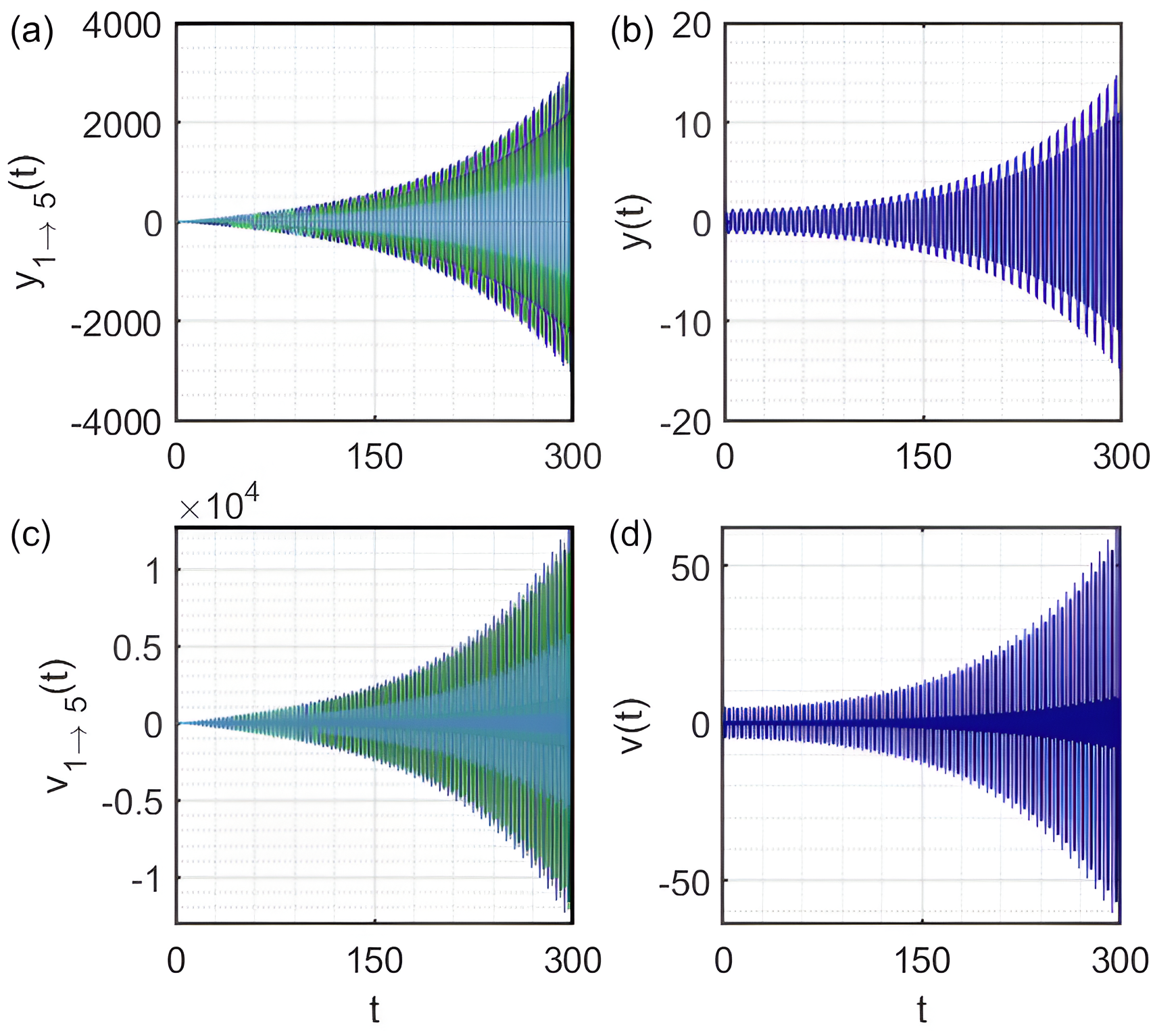
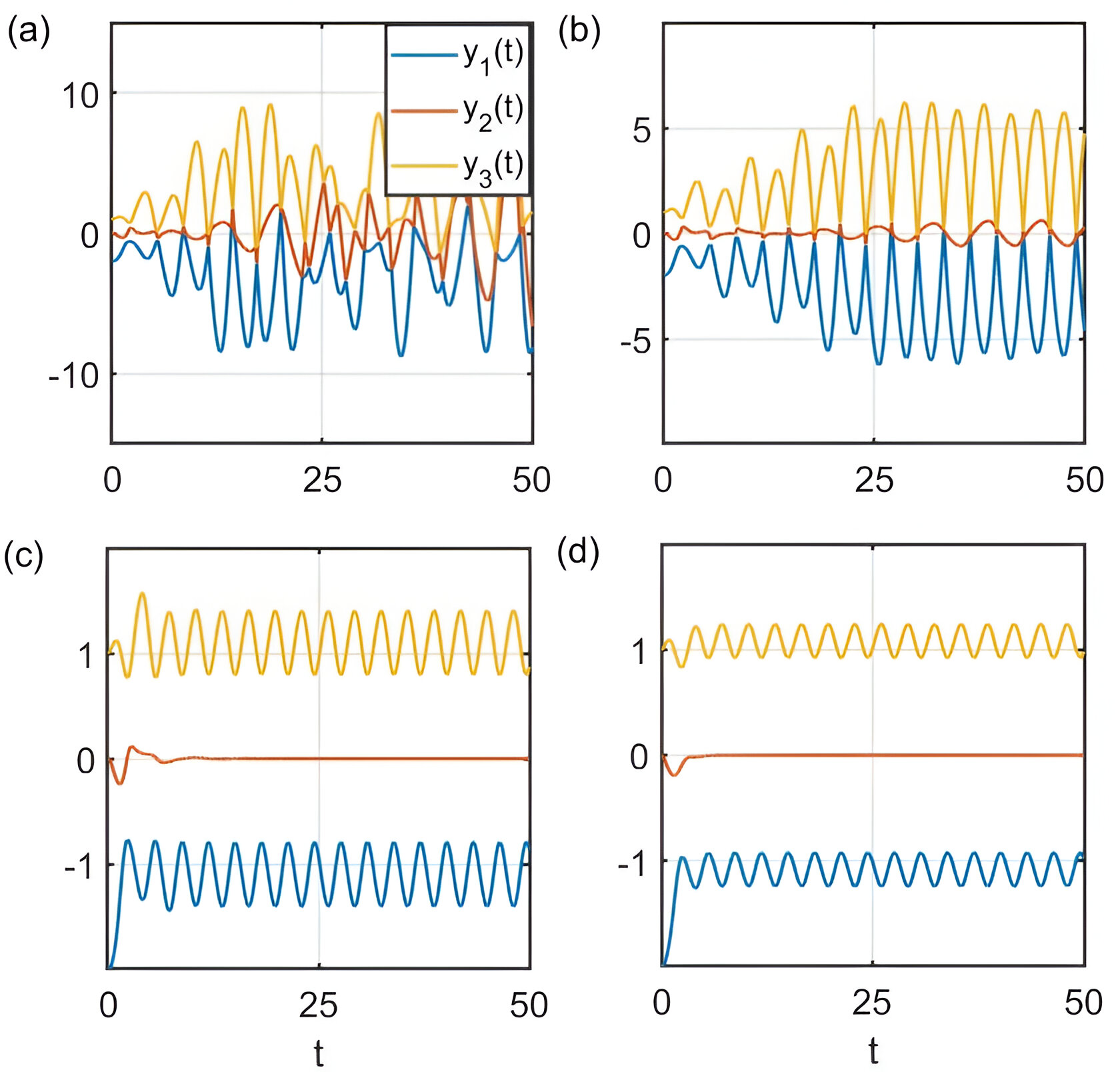
Finally, we are in a position to understand the role of Coulomb interaction on the stability and the phase chart in this model using the following argument. Let us assume that the system is unstable. In this case, approaches infinity, as observed in the single particle Mathieu equation. When the distance between the ions is sufficiently large, the Coulomb interaction is negligible, thus the instability of this model should be fully determined by the phase chart of the single particle Mathieu model. Thus, we have sufficient reasons to believe that the phase chart in this interacting Mathieu model should be the same as the single particle Mathieu equation. This is shown in Fig. 12, however, the dynamics can still be fundamentally different. In Fig. 12, we focus on the motion and the velocity in the unstable region for two groups of ions. The first group is composed of 5 ions in Fig. 12 (a) and (c), and the second group is composed of single ion in Fig. 12 (b) and (d). Both systems will oscillate exponentially, but have different magnitudes. The difference between the amplitude of the motion of the first ion and the fifth ion is around , however, the difference between their velocities is around the order of . The vibration magnitude of the position and the velocity are much smaller in a single particle model. Despite of this difference, both systems display similar patterns of oscillations. When a group of ions are sufficiently far from each other, the Coulomb forces decrease rapidly to zero, resulting in no influence on their motion. In such cases, the ions act like independent particles, which gives rise to a collective behavior similar to that of a single particle.
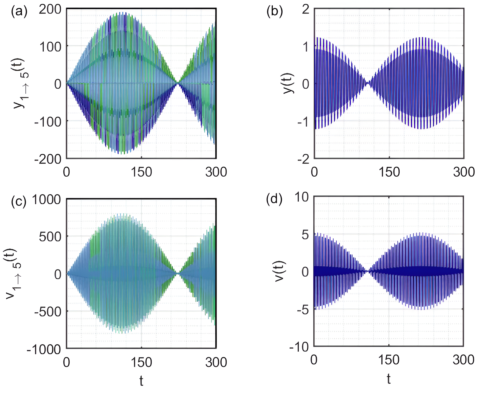
Next, we study the motion and the velocity of 5 ions and of 1 ion in the stable region, which are presented in Fig. 13, with and . Similar features have also been observed. We find that these two conditions have the same parameters and they have the same stability. However, in the many-body model, the vibration amplitude is greatly enhanced by about two orders of magnitude, as compared with the single particle one. This result also means that in the many-body model the larger is, the larger the vibration amplitude will be. For this reason, the trapping of particles (where is large) without damping will become a significant issue. However, in the presence of damping, the enhanced vibration amplitude will be greatly suppressed.
This observed phenomenon is fascinating in physics, because of the fact that the collective interactions of multiple particles give rise to behaviors similar to those of individual particles. This parallelism highlights not only the fundamental principles regarding the behavior of trapped ion systems, but also the interconnections of their dynamics. We hope these physics can be observed in experiments van Mourik et al. (2022). In the case of strong damping, the single particle will cease to oscillate, yet the many-body one will oscillate around its equilibrium position, with position and amplitude satisfying Eq. 32.
VI Mathieu equation with cubic anharmonic term
The Mathieu equation with a cubic nonlinear term, in the presence of many trapped ions can be written as El-Dib (2024); Pagano et al. (2018)
| (52) |
where is the anharmonic coefficient. The cubic nonlinear coefficient introduces a nonlinearity to the equation. Therefore, the response of the system will no longer be directly proportional to the applied force, which naturally will make the system exhibit much more complicated behaviors. The cubic nonlinear coefficient in the Mathieu equation for trapped ions typically originates from the anharmonicity in the trapping potential that is responsible of the interaction between the ion’s motion and the trapping field Moatimid (2020); Kidachi and Onogi (1997). Numerical calculations show that in the presence of a weak , the vibration amplitude is
| (53) |
thus for all and the system is always stable. This relation can be determined by the minimal of , with , yielding . Hence the cubic nonlinear term can fundamentally change the fate of the phase chart discussed before. In the following, we are interested in the effect of this nonlinear term on the vibration amplitude with strong damping.
In this section, we will explore the effect of the nonlinear term on the collisions of ions. Assume to be the vibration amplitude, then we require
| (54) |
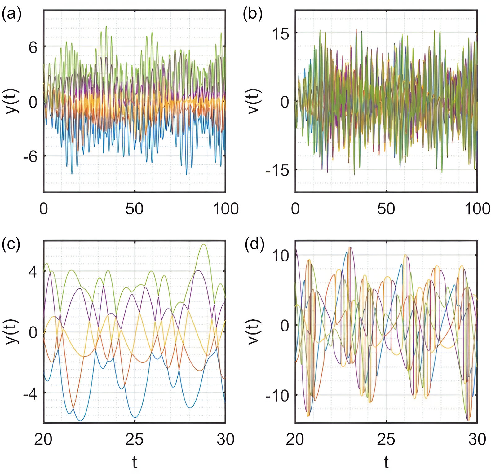
in which condition the nonlinear term is important. By solving Eq. 52, with , we present the dynamics of 5 trapped ions in Fig. 14. While the pattern of the ions looks organized, the pattern of the velocities is not. As compared with Fig. 9, we find that the quasi-periodic dynamics no longer exists. Moreover, the exchange of velocities between the first and the last ion will not be observed; instead, the collision of ions will happen at different times (see Fig. 14 (c) and (d)), leading to an exchange of velocities between adjacent ions. For this reason, the synchronization dynamics are not observed anymore. This is a typical feature in a nonlinear trap Pagano et al. (2018), in which the ions in different positions may feel some slightly different trapping frequency, therefore their dynamics and period will be different. We find that when , the synchronization and the associated exchange of velocities can still be observed. However, in the much stronger nonlinear trap, the dynamics will become much more complicated. Furthermore, in the case of strong damping, the ions will vibrate around their equilibrium positions, leading to periodic dynamics, as observed in Sec. III. In this case, the positions of ions may appear to have different vibration amplitudes and different effective periods. Thus, the synchronization comes from the parametric driving field and the harmonic potential, in which all ions tend to have the same behavior, including the same relative phase, which maybe measured in the future experiments.
VII Experiments and possible signatures
When working with numerical simulations, it is necessary to use dimensionless variables to simplify the equations and reducing the complexity of the problem. However, to interpret these numerical results in real life, it is crucial to convert these dimensionless variables back into dimensional terms, and estimate their values. Therefore, we will have to estimate the values of , and possibly to be used in experiments.
In a Paul trap, there is typically both a dc and an RF voltages applied to the electrode. Therefore, the total voltage should be . Created by this total voltage is the electric potential, which in one dimension reads as Trimby et al. (2022); Noshad and Doroudi (2009); Romaszko et al. (2020); Zhao and Krstic (2008); Poindron et al. (2023)
| (55) |
then, the electric field can be defined as , which will allow us to find the equation of motion of the ions using , yielding Ziaeian and Noshad (2010); Chu et al. (1998); Drewsen and Brøner (2000); Paul (1990); Noshad and Kariman (2011); Ziaeian et al. (2011).
| (56) |
Therefore, the expression of the parameters in the dimensional system Leibfried et al. (2003); Dawson and Douglas (2010); Zhao et al. (2002); March (2006); Seddighi Chaharborj et al. (2012); Drewsen and Brøner (2000); Dawson and Douglas (2010)
| (57) |
Here, is the charge of the ions, is the applied dc voltage, is the applied radio-frequency voltage, is the mass of the ions, is the system frequency, is the driving force frequency and is a parameter that defines the geometry of the trap and represents the distance from the trap center to the electrode.
In an experimental setup for the trapped ions, the system is bound to experience some heating effect due to many reason, like collisions between the ions, exchange of energy with the environment, and fluctuations of the applied electric fields. Therefore, the trapped ions need to be cooled down, in order to maintain its stability. Many techniques can be used for this. In Refs. van Mourik et al. (2022); Ziaeian and Noshad (2010); Kaplan (2009), two different mechanisms for the damping force were discussed, the first one is the drag force due to residual rarefied gas, and the other one is the interaction with the blue-detuned laser beams. In both cases, the damping rate can be tuned in a wide range and in general the damping from the laser field dominates by Doppler effect. Especially, this damping force is essential for the cooling of trapped ions. That is why a damping term was introduced in Eq. 56. Furthermore, and can be estimated knowing the values of experimental variables , , , and . Using the above relations, we get
| (58) |
which can be tuned in a wide range of experiments. Furthermore, using Eq. 32, the strong damping regime can be achieved when , yielding
| (59) |
Thus, we expect the physics discussed in this work to be researched using trapped ions. For example, in experiment with trapped 171Yb+ ions with kHz Yan et al. (2022); Trimby et al. (2022), with V, mm, eVm, and MeV, and MHz, we can obtain
| (60) |
The similar magnitude of can be obtained using Eq. 58 by changing of . Much more details can be found in Ref. Trimby et al. (2022). Obviously, these values can be tuned in a wide range in experiments, thus the phase chart can be studied using this platform. From Eq. 59, we require , assuming , and from , we expect that the cooling of the trapped ions can be reached in the time scale of in the strong damping limit; see Fig. 5 and Fig. 11.
VIII Conclusions
To summarize, we present a complete analysis of the interacting Mathieu equation with the Coulomb interaction, which can be realized using trapped ions. We investigate the physics in various conditions. In the strong damping limit, the dynamics can be solved using perturbation theory, showing that the damping coefficient can play the role of reducing the vibration amplitude about their equilibrium positions. In the weak damping limit, we observe the synchronization dynamics and the associated exchange of velocities between distant trapped ions, which resembles to the dynamics of Newton’s cradle. In this case, the phase chart for the stability and instability dynamics is independent of the Coulomb interaction, thus, it is the same as the single particle Mathieu equation. Finally, we study the effect of the nonlinear anharmonic term in the trapping potential, in which the system will always be stable for all the parameters. In this case, the desynchronization prohibits the exchange of velocities between distant ions. We estimated that these results are within the reach of the current experiments with trapped ions and expect these interesting dynamics to be observed.
During the preparing of this work, we were constantly asking the fundamental question of what are the most unique features in this many-body classical model? The generalization of the exact solvable single particle Mathieu equation to the many-body models and even to the quantum realms are quite obviously important and necessary Leibfried et al. (2003); Singer et al. (2010), which should exhibit some interesting physics. In most of cases, the quasi-periodic solutions are the major concern in these investigations. From these investigations with the Coulomb interaction in this work, it was quite possible to provide some concrete answers to our previous question, which are, synchronization dynamics with coherent phases, collision-induced exchange of velocity, desynchronization dynamics from the anharmonic effect, and periodic oscillations in the strong damping limits. These results are not limited to small amplitude vibrations. Some of these results may be beyond the scope of the Mathieu equation (thus without the Floquet theorem), indicating the necessary investigation of the interacting Mathieu equation in future. These results can be found for other types of inter-particle interactions (including Van der Waals interactions) Trimby et al. (2022), in which when , . It is important that some of these predictions can be immediately verified in experiments.
Finally, this work contribute to the study of the dynamics of trapped ions, which can be generalized to higher dimensions Porras and Cirac (2006); Jordan et al. (2019); Wu and Duan (2020); Guo et al. (2024), due to the current research of trapped ions for quantum computations. The interacting Mathieu equation is probably much more important due to the wide range study of this model in dynamical systems in terms of the Floquet theorem in mathematics. It is to be hoped that the experimental progresses for the realization of this model can stimulate the investigation of this interacting Mathieu model from a pure mathematical perspective beyond the quasi-periodic solutions Jiansheng and Yingfei (2007); Ge et al. (2022). Meanwhile, this model is also interesting in the presence of noise at finite temperature with both dissipation and fluctuation, which is connected by the Einstein relation in the Brownian motion between the temperature, damping rate and diffusion constant, which is always presented in experiments when the temperature is not sufficiently low Wen et al. (2023); Keller J. and H (2013); Ulm et al. (2013).
Acknowledgments: We thank Prof. Ping Xing Chen and Prof. Dun Zhou for the valuable discussions about the physical realization of this model and about its possible applications in pure mathematics. This work is supported by Innovation Program for Quantum Science and Technology (No. 2021ZD0301200, No. 2021ZD0303200, and No. 2021ZD0301500) and the Alliance of International Science Organizations (ANSO).
References
- Ruby (1996) Lawrence Ruby, “Applications of the Mathieu equation,” Am. J. Phys. 64, 39–44 (1996).
- Bibby and Peterson (2013) Malcolm Bibby and Andrew F. Peterson, “Accurate computation of mathieu functions,” in Accurate Computation of Mathieu Functions (2013).
- Mathieu (1868) Émile Mathieu, “Mémoire sur le mouvement vibratoire d’une membrane de forme elliptique.” J. Math. Pures Appl. 13, 137 (1868).
- Paul (1990) Wolfgang Paul, “Electromagnetic traps for charged and neutral particles,” Rev. Mod. Phys. 62, 531–540 (1990).
- Landau and Lifshitz (1976) L. D. Landau and E. M. Lifshitz, Mechanics, Third Edition: Volume 1 (Course of Theoretical Physics), 3rd ed. (Butterworth-Heinemann, 1976).
- Bhattacharjee et al. (2007) Jayanta Bhattacharjee, A. Mallik, and Sagar Chakraborty, “An introduction to nonlinear oscillators: A pedagogical review,” Indian J. Phys. 81, 1115–1175 (2007).
- Richards (1983) J. A. Richards, “The mathieu equation,” in Analysis of Periodically Time-Varying Systems (Springer Berlin Heidelberg, Berlin, Heidelberg, 1983) pp. 93–107.
- Note (1) For example, let us consider the following ordinary differential equation , with solution , which is not a periodic solution of . However, it is a quasi-periodic solution satisfying , as expected from the Floquet theorem.
- Parra-Verde and Gutiérrez-Vega (2024) Erick R. Parra-Verde and Julio C. Gutiérrez-Vega, “Steady-state solutions of the whittaker–hill equation of fractional order,” Commun. Nonlinear Sci. Numer. Simul. 131, 107812 (2024).
- Urwin and Arscott (1970) Kathleen M. Urwin and F. M. Arscott, “Iii.—theory of the whittaker hill equation,” Proc. R. Soc. Edinb. A Math. Phys. Sci. 69, 28 (1970).
- Koenig (1933) Harold D. Koenig, “Calculation of characteristic values for periodic potentials,” Phys. Rev. 44, 657–665 (1933).
- Daniel (2020) Derek J. Daniel, “Exact solutions of Mathieu’s equation,” Prog. Theor. Exp. Phys. 2020, 043A01 (2020).
- Sinclair (2014) Alastair Sinclair, An Introduction to Trapped Ions, Scalability and Quantum Metrology (Springer, 2014).
- Cirac and Zoller (2000) J. Cirac and P. Zoller, “A scalable quantum computer with ions in an array of microtraps,” Nature 404, 579–581 (2000), 10.1038/35007021.
- Steven Ban and Wen (2016) Peter Chang Steven Ban, Matthew Bledsoe and Garrett Wen, “Constructing a paul trap for undergraduate laboratories,” (2016).
- Cirac and P. (1995) J. I. Cirac and Zoller P., “Quantum computations with cold trapped ions,” Phys. Rev. Lett. 74, 4091–4094 (1995).
- Leibfried et al. (2003) D. Leibfried, R. Blatt, C. Monroe, and D. Wineland, “Quantum dynamics of single trapped ions,” Rev. Mod. Phys. 75, 281–324 (2003).
- Savaryn et al. (2016) John Savaryn, Timothy Toby, and Neil Kelleher, “A researcher’s guide to mass spectrometry‐based proteomics,” Proteomics 16 (2016), 10.1002/pmic.201600113.
- Thompson et al. (2002) R I Thompson, T J Harmon, and M G Ball, “The rotating-saddle trap: a mechanical analogy to rf-electric-quadrupole ion trapping?” Can. J. Phys. 80, 1433–1448 (2002).
- Wu and Diebold (2012) Binbin Wu and Gerald J. Diebold, “Mathieu function solutions for photoacoustic waves in sinusoidal one-dimensional structures,” Phys. Rev. E 86, 016602 (2012).
- Trypogeorgos and Foot (2016) Dimitris Trypogeorgos and Christopher J. Foot, “Cotrapping different species in ion traps using multiple radio frequencies,” Phys. Rev. A 94, 023609 (2016).
- Kovacic et al. (2018) Ivana Kovacic, Richard Rand, and Si Mohamed Sah, “Mathieu’s equation and its generalizations: Overview of stability charts and their features (review article),” Appl. Mech. Rev. 70, 020802 (2018).
- Stafford et al. (1984) G.C. Stafford, P.E. Kelley, J.E.P. Syka, W.E. Reynolds, and J.F.J. Todd, “Recent improvements in and analytical applications of advanced ion trap technology,” Int. J. Mass Spectrom. Ion Processes. 60, 85–98 (1984).
- Richards (1976) J. A. Richards, “Stability diagram approximation for the lossy mathieu equation,” SIAM J. Appl. Math. 30, 240–247 (1976).
- Acar and Feeny (2016) G. Acar and B. F. Feeny, “Floquet-Based Analysis of General Responses of the Mathieu Equation.” ASME. J. Vib. Acoust. 138 (2016).
- Turyn (1993) Lawrence Turyn, “The damped Mathieu equation,” Quart. Appl. Math. 51 (1993).
- Sinha and David (2001) S.C. Sinha and A. David, “Parametric excitation,” in Encyclopedia of Vibration, edited by S. Braun (Elsevier, Oxford, 2001) pp. 1001–1009.
- Wilkinson et al. (2018) Samuel A. Wilkinson, Nicolas Vogt, Dmitry S. Golubev, and Jared H. Cole, “Approximate solutions to mathieu’s equation,” Physica E 100, 24–30 (2018).
- Jia et al. (2016) Yu Jia, Sijun Du, and Ashwin Seshia, “Twenty-eight orders of parametric resonance in a microelectromechanical device for multi-band vibration energy harvesting,” Sci. Rep. 6, 30167 (2016).
- Koad et al. (2023) Peeravit Koad, Jatechan Channuie, and Phongpichit Channuie, “On preheating after inflation in scalar-tensor theories of gravity,” Fortsch. Phys. 71, 2300041 (2023).
- Nop et al. (2023) Gavin N. Nop, Jonathan D. H. Smith, Daniel Stick, and Durga Paudyal, “Novel ion trap junction design for transporting qubits in a 2d array,” (2023), 2310.07195 .
- Rand (2012) Richard Rand, “Lecture notes on nonlinear vibrations,” (2012).
- Insperger and Stepan (2003) T. Insperger and G. Stepan, “Stability of the Damped Mathieu Equation With Time Delay ,” J. Dyn. Syst. Meas. Control. 125, 166–171 (2003).
- Taylor and Narendra (1969) James H. Taylor and Kumpati S. Narendra, “Stability regions for the damped mathieu equation,” SIAM J. Appl. Math. 17, 343–352 (1969).
- Konenkov et al. (2002) N.V. Konenkov, M. Sudakov, and D.J. Douglas, “Matrix methods for the calculation of stability diagrams in quadrupole mass spectrometry,” J. Am. Soc. Mass Spectrom. 13, 597–613 (2002).
- Poulin and Flierl (2008) Francis Poulin and Glenn Flierl, “The stochastic mathieu’s equation,” Proc. R. Soc. A. 464, 1885–1904 (2008).
- van Mourik et al. (2022) Martin W. van Mourik, Pavel Hrmo, Lukas Gerster, Benjamin Wilhelm, Rainer Blatt, Philipp Schindler, and Thomas Monz, “rf-induced heating dynamics of noncrystallized trapped ions,” Phys. Rev. A 105, 033101 (2022).
- El-Dib (2024) Yusry O. El-Dib, “An innovative efficient approach to solving damped mathieu–duffing equation with the non-perturbative technique,” Commun. Nonlinear Sci. Numer. Simul. 128, 107590 (2024).
- Pagano et al. (2018) G Pagano, P W Hess, H B Kaplan, W L Tan, P Richerme, P Becker, A Kyprianidis, J Zhang, E Birckelbaw, M R Hernandez, Y Wu, and C Monroe, “Cryogenic trapped-ion system for large scale quantum simulation,” Quantum Science and Technology 4, 014004 (2018).
- Moatimid (2020) Galal M. Moatimid, “Stability analysis of a parametric duffing oscillator,” J. Eng. Mech. 146, 05020001 (2020).
- Kidachi and Onogi (1997) Hideyuki Kidachi and Hiroshi Onogi, “Note on the Stability of the Nonlinear Mathieu Equation,” Prog. Theor. Phys. 98, 755–773 (1997).
- Trimby et al. (2022) E Trimby, H Hirzler, H Fürst, A Safavi-Naini, R Gerritsma, and R S Lous, “Buffer gas cooling of ions in radio-frequency traps using ultracold atoms,” New J. Phys. 24, 035004 (2022).
- Noshad and Doroudi (2009) Houshyar Noshad and Alireza Doroudi, “Computation of five stability regions in a quadrupole ion trap using the fifth-order runge–kutta method,” Int. J. Mass Spectrom. 281, 79–81 (2009).
- Romaszko et al. (2020) Zak David Romaszko, Seokjun Hong, Martin Siegele, Reuben Kahan Puddy, Foni Raphaël Lebrun-Gallagher, Sebastian Weidt, and Winfried Karl Hensinger, “Engineering of microfabricated ion traps and integration of advanced on-chip features,” Nat. Rev. Phys. 2, 285–299 (2020), 1908.00267 .
- Zhao and Krstic (2008) Xiongce Zhao and Predrag Krstic, “Molecular dynamics simulation study on trapping ions in a nanoscale paul trap,” Nanotechnology 19, 195702 (2008).
- Poindron et al. (2023) A. Poindron, J. Pedregosa-Gutierrez, and C. Champenois, “Thermal bistability in laser-cooled trapped ions,” Phys. Rev. A 108, 013109 (2023).
- Ziaeian and Noshad (2010) Iman Ziaeian and Houshyar Noshad, “Theoretical study of the effect of damping force on higher stability regions in a Paul trap,” Int. J. Mass Spectrom. 289, 1–5 (2010).
- Chu et al. (1998) X.Z. Chu, M. Holzki, R. Alheit, and G. Weitha, “Observation of high-order motional resonances of an ion cloud in a paul trap,” Int. J. Mass Spectrom. Ion Processes. 173, 107–112 (1998).
- Drewsen and Brøner (2000) M. Drewsen and A. Brøner, “Harmonic linear paul trap: Stability diagram and effective potentials,” Phys. Rev. A 62, 045401 (2000).
- Noshad and Kariman (2011) Houshyar Noshad and Behjat-Sadat Kariman, “Numerical investigation of stability regions in a cylindrical ion trap,” Int. J. Mass Spectrom. 308, 109–113 (2011).
- Ziaeian et al. (2011) I. Ziaeian, S.M. Sadat Kiai, M. Ellahi, S. Sheibani, A. Safarian, and S. Farhangi, “Theoretical study of the effect of ion trap geometry on the dynamic behavior of ions in a paul trap,” Int. J. Mass Spectrom. 304, 25–28 (2011).
- Dawson and Douglas (2010) P.H. Dawson and D.J. Douglas, “Quadrupoles, use of in mass spectrometry,” Encycl. Spectrosc. Spectrom. , 2315–2324 (2010).
- Zhao et al. (2002) X. Zhao, V. L. Ryjkov, and H. A. Schuessler, “Parametric excitations of trapped ions in a linear rf ion trap,” Phys. Rev. A 66, 063414 (2002).
- March (2006) Raymond E. March, “Quadrupole ion trap mass spectrometer,” in Encyclopedia of Analytical Chemistry (John Wiley and Sons, Ltd, 2006).
- Seddighi Chaharborj et al. (2012) Sarkhosh Seddighi Chaharborj, Pei See Phang, Seyed sadat kiai, Zanariah Abdul Majid, Mohd Bakar, and I.fudziah Ismail, “Study of a quadrupole ion trap with damping force by the two-point one block method,” Rapid Commun. Mass Spectrom. 26, 1481–7 (2012).
- Ziaeian and Noshad (2010) Iman Ziaeian and Houshyar Noshad, “Theoretical study of the effect of damping force on higher stability regions in a paul trap,” Int. J. Mass Spectrom. 289, 1–5 (2010).
- Kaplan (2009) A. E. Kaplan, “Single-particle motional oscillator powered by laser,” Opt. Express 17, 10035–10043 (2009).
- Yan et al. (2022) Chen Yan, Ban Yue, He Ran, Cui Jin-Ming, Huang Yun-Feng, Li Chuan-Feng, Guo Guangcan, and Jorge Casanova, “A neural network assisted 171yb+ quantum magnetometer,” pj Quantum Information 8, 152 (2022).
- Singer et al. (2010) Kilian Singer, Ulrich Poschinger, Michael Murphy, Peter Ivanov, Frank Ziesel, Tommaso Calarco, and Ferdinand Schmidt-Kaler, “Colloquium: Trapped ions as quantum bits: Essential numerical tools,” Rev. Mod. Phys. 82, 2609–2632 (2010).
- Porras and Cirac (2006) D. Porras and J. I. Cirac, “Quantum manipulation of trapped ions in two dimensional coulomb crystals,” Phys. Rev. Lett. 96, 250501 (2006).
- Jordan et al. (2019) Elena Jordan, Kevin A. Gilmore, Athreya Shankar, Arghavan Safavi-Naini, Justin G. Bohnet, Murray J. Holland, and John J. Bollinger, “Near ground-state cooling of two-dimensional trapped-ion crystals with more than 100 ions,” Phys. Rev. Lett. 122, 053603 (2019).
- Wu and Duan (2020) Y.-K. Wu and L.-M. Duan, “A two-dimensional architecture for fast large-scale trapped-ion quantum computing,” Chinese Physics Letters 37, 070302 (2020).
- Guo et al. (2024) S-A Guo, Y.-K. Wu, J Ye, L Zhang, Wenqian Lian, R. Yao, Y. Wang, R.-Y. Yan, Y.-J. Yi, Y.-L. Xu, B.-W. Li, Y.-H. Hou, Y.-Z. Xu, W.-X. Guo, C. Zhang, Bin Qi, Z-C Zhou, Liqiang He, and Lu-Ming Duan, “A site-resolved 2d quantum simulator with hundreds of trapped ions,” Nature 23456, 234234 (2024).
- Jiansheng and Yingfei (2007) Geng Jiansheng and Yi Yingfei, “Quasi-periodic solutions in a nonlinear schrödinger equation,” Journal of Differential Equations 233, 512–542 (2007).
- Ge et al. (2022) Chuanfang Ge, Jiansheng Geng, and Yingfei Yi, “Quasi-periodic breathers in Newton’s cradle,” Journal of Mathematical Physics 63, 082703 (2022).
- Wen et al. (2023) Wei Wen, Shanhua Zhu, Yi Xie, Baoquan Ou, Wei Wu, Pingxing Chen, Ming Gong, and Guangcan Guo, “Generalized Kibble-Zurek mechanism for defects formation in trapped ions,” Science China Physics, Mechanics, and Astronomy 66, 280311 (2023).
- Keller J. and H (2013) Pyka K. Keller J. and Partner H, “Topological defect formation and spontaneous symmetry breaking in ion coulomb crystals,” Nat. Commun. 4, 2291 (2013), 10.1038/ncomms3291.
- Ulm et al. (2013) S. Ulm, J. Ronagel, G. Jacob, C. Degünther, S. T. Dawkins, U. G. Poschinger, R. Nigmatullin, A. Retzker, M. B. Plenio, F. Schmidt-Kaler, and K. Singer, “Observation of the kibble–zurek scaling law for defect formation in ion crystals,” Nat. Commu 4, 2290 (2013).