Immiscible Diffusion: Accelerating Diffusion Training with Noise Assignment

Abstract

In this paper, we point out suboptimal noise-data mapping leads to slow training of diffusion models. During diffusion training, current methods diffuse each image across the entire noise space, resulting in a mixture of all images at every point in the noise layer. We emphasize that this random mixture of noise-data mapping complicates the optimization of the denoising function in diffusion models. Drawing inspiration from the immiscible phenomenon in physics, we propose Immiscible Diffusion, a simple and effective method to improve the random mixture of noise-data mapping. In physics, miscibility can vary according to various intermolecular forces. Thus, immiscibility means that the mixing of the molecular sources is distinguishable. Inspired by this concept, we propose an assignment-then-diffusion training strategy. Specifically, prior to diffusing the image data into noise, we assign diffusion target noise for the image data by minimizing the total image-noise pair distance in a mini-batch. The assignment functions analogously to external forces to separate the diffuse-able areas of images, thus mitigating the inherent difficulties in diffusion training. Our approach is remarkably simple, requiring only one line of code to restrict the diffuse-able area for each image while preserving the Gaussian distribution of noise. This ensures that each image is projected only to nearby noise. To address the high complexity of the assignment algorithm, we employs a quantized-assignment strategy, which significantly reduces the computational overhead to a negligible level (e.g., 22.8ms for a large batch size of 1024 on an A6000). Experiments demonstrate that our method can achieve up to 3x faster training for consistency models and DDIM on the CIFAR dataset, and up to 1.3x faster on CelebA datasets for consistency models. Besides, we conduct thorough analysis about the Immiscible Diffusion, which sheds lights on how it improves diffusion training speed while improving the fidelity. The code is available at https://yhli123.github.io/immiscible-diffusion

Figure 1: Immiscible Diffusion uses a single line of code to efficiently re-assign a batch of noise to images. This process results in only a 2% reduction in distance post-assignment, leading to up to 3x increased training efficiency while maintaining a reasonable FID on top of the Consistency Model for CIFAR Dataset. Additionally, Immiscible Diffusion significantly enhances the image quality of Stable Diffusion for both unconditional and conditional generation tasks on ImageNet Dataset within the same number of training steps.

1 Introduction

The diffusion model has made impressive progress in image generation by framing the process as a phase of denoising random Gaussian noise into the final image. Despite the advancements, training a diffusion model is resource-intensive. For example, even on the primary image dataset CIFAR-10, the representative few-step diffusion model, Consistency Model [38], requires training for 10 days on 4 A6000 GPUs to reach a desired FID score of around 10. Similarly, with fewer model parameters, multiple-step diffusion model DDIM [35] still requires 24 hours on an A5000 GPU on the CIFAR-10 dataset. Although recent remarkable achievements in accelerating the inference of diffusion models [13, 25, 38, 20, 22, 23] have been accomplished, the inefficiency of diffusion training remains a significant bottleneck, hindering the iterative development of vision generative AI.

Previous methods to improve diffusion training have focused on various strategies, such as balancing the impact of activation layers and neural weights [11], modifying the hyperparameters and design choices [37], and leveraging patchifying strategies [43] etc. Specifically, Karras et al. [11] modifies the activation magnitude, neural weight standardization, and group normalization, achieving significant acceleration in diffusion training. Besides, previous work [37] proposes a customized method for consistency model to improve the performance and diffusion training. Our method is orthogonal to these previous methods. We got inspired by the Immiscible Diffusion in physics. As illustrated in Fig. 2, miscible particles tightly jumble together during the diffusion process, making it difficult to separate them individually during denoising phase. However, when the particles are rendered immiscible, they can still achieve a similar overall distribution while remaining clearly distinguishable (see the shape of the two images at the right of Fig. 2). This insight informs our strategy for improving the disentanglement of diffused data.

We draw an analogy from the phenomenon of Immiscible Diffusion and relate the distribution of image data to the behavior of particles discussed above. In traditional diffusion processes, each image can be diffused to any point in the noise space, and conversely, each point in the noise space can be denoised to any source image, as illustrated in the left image of Fig. 2 (b). We hypothesize that the jumbled image-noise mapping creates a miscible diffusion effect and makes the optimization of diffusion model difficult. Inspired by the Immiscible Diffusion, we are motivated to make the mixed diffusion phase distinguishable.

Figure 2: Physical illustration of Immiscible Diffusion. (a) depict the miscible and Immiscible Diffusion phenomenon in physics, while (b) demonstrate the image-noise pair relation in traditional (miscible) and Immiscible Diffusion method.

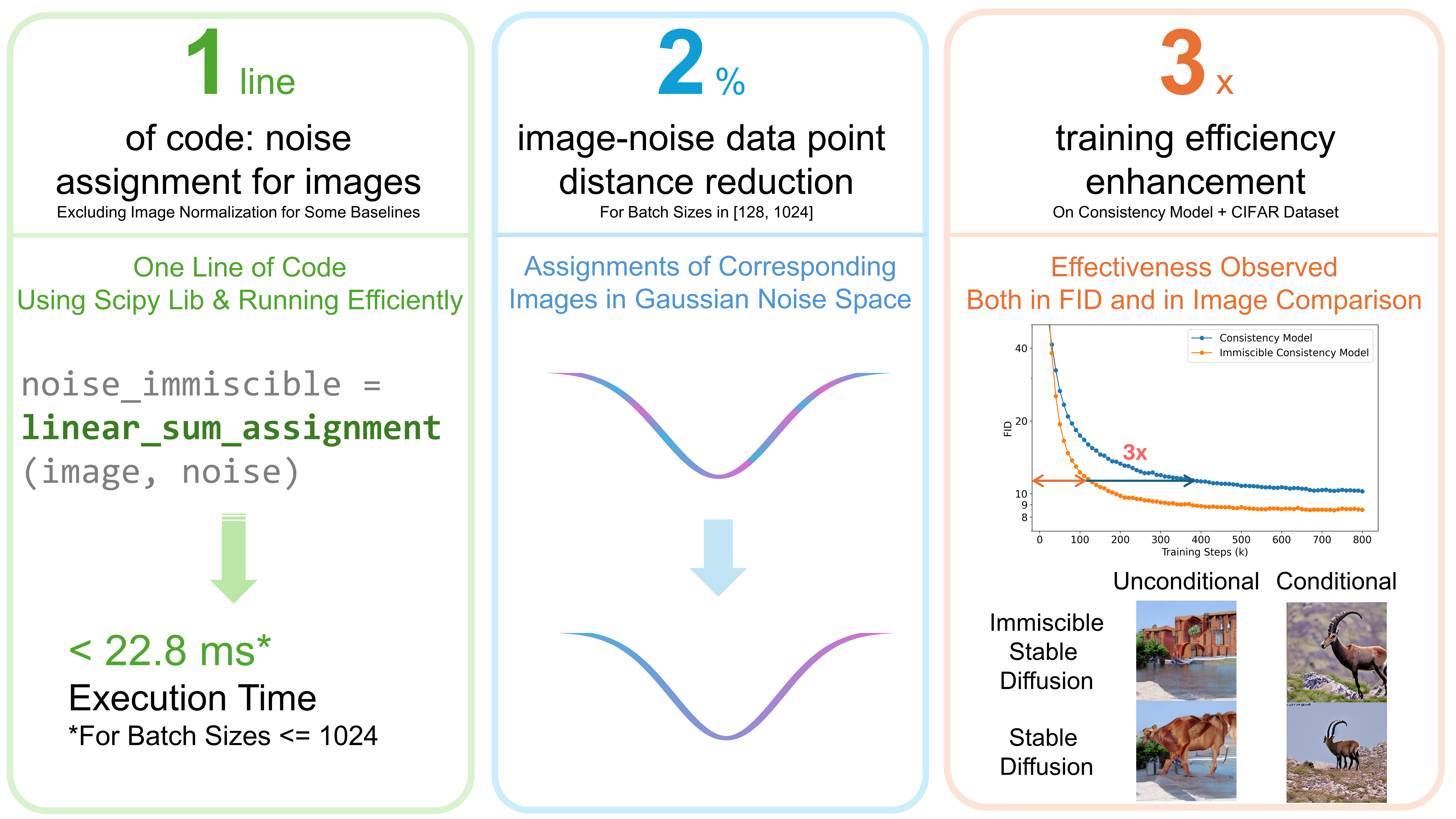
We propose a simple and novel Immiscible Diffusion method. Note that we still sample Gaussian noise but perform a batch-wise assignment of noise to each image based on the distance between them during training. This approach ensures that each image is only diffused to surrounding areas while maintaining the overall Gaussian distribution of all noises. This noise assignment makes the diffusion model especially effective at denoising at high noise levels, which benefits the current trend of few-step denoising models. However, technically, the image data-noise assignment is an O($N^{2}logN$)-O($N^{3}$) operation, which introduces significant overhead during training, especially for large-scale training with huge batch sizes and high-resolution images. To address this, we employ a novel quantization method during assignment. We quantize the noise and image data into low-precision formats (e.g., 16-bit) during conducting the assignment algorithm. We highlight our method only involves one line of code, and is only performed during the training phase without modifying the model architecture, the noise scheduler, the sampler, or the method of inference.

We conduct experiments on three diffusion baselines, Consistency models, DDIM and Stable Diffusion on the CIFAR-10, CelebA and ImageNet datasets. Results show that our proposed method significantly improves the training efficiency in all experiments. Specifically, we achieve 3x training efficiency for CIFAR-10 dataset with immiscible consistency model compared to the traditional consistency one. Furthermore, we show the FID is even lower with our method used, confirming the fidelity of our generated images. We also provide images generated from models trained with traditional and immiscible models experiencing the same training steps, where we see those from immiscible models are much more complete and clearer, further proving the training efficiency enhancement resulted from the Immiscible Diffusion. Examples are shown in Fig. 1 right. Deeper analysis shows that our method, though with only one line of code and involving 2̃% image-noise datapoint distance changes, achieves all the benefits above in a negligible running time.

To sum up, our contributions are as follows:

• We identify the issue of the image-noise matching relation, which leads to the slow convergence of diffusion training.

• We propose a simple and effective method, Immiscible Diffusion, a strategy that only requires one-line of code, to improve training efficiency for diffusion training.

• Experiments demonstrate the effectiveness of our proposed method on several popular diffusion models across multiple datasets. Additionally, we conduct thorough analyses and ablation studies to elucidate how our method works.

2 Related Work

2.1 Diffusion Model with Efficient Inference

Diffusion models [39, 9, 30, 27] have been attracting huge attention because of its high-fidelity image and video generation [8, 10, 26], its data-efficient perception [40, 24, 44], and even its representation ability for robotics [2, 28, 1]. However, the slow inference is one of the key bottlenecks for diffusion models. To address this issue, various approaches have been proposed. For instance, techniques such as DDIM [35] have reduced the number of denoising steps from 1000 to 10, significantly speeding up the process. Furthermore, the introduction of consistency models [38] and LCM [25], which utilize the properties of a self-consistency, enables denoising in as few as 1-4 steps, further enhancing the generation speed of diffusion models. Subsequently, the development of SD-turbo [33], which leverages GAN [6] loss for high-definition image generation in a single step. The Consistency Trajectory Models [12, 29] improve the generation quality of consistency models, accelerate research on efficient inference for diffusion models. Additionally, beyond reducing denoising steps, efforts to improve inference efficiency of single function evaluation are being explored in various ways, including model quantization [19], and partitioning the generative components [18]. Moreover, StreamDiffusion [13] streamlines denoising steps to achieve real-time inference at the pipeline level optimization. The improvement of the inference efficiency significantly pushes forward the real applications based on Diffusion Models. Yet accelerating diffusion training is still under-explored.

2.2 Diffusion Model with Efficient Training

Improving the training efficiency of diffusion models is crucial. Various strategies have been proposed, including architectural modifications [11], approximating the diffusion phase with flow [20], and designing parameter choices [37] etc. Specifically, in [11], the authors discover that the magnitude of activation and the magnitude of neural weights significantly impact the training dynamics of diffusion models. They propose adjusting the activation magnitude and standardizing neural weights, as well as modifying the normalization layers to make the diffusion training in a more smooth dynamic. Besides, Song et al. [37] aim to enhance the training efficiency of consistency models through customized design choices, significantly improving both training speed and fidelity. Furthermore, leveraging approximation strategies based on ODE assumptions [20] improves not only inference efficiency but also training efficiency since diffusion trajectories is prone to deterministic. Beyond improving the diffusion training with either adjusting architecture or selecting parameters, Wang et al. [43] introduce a novel patch strategy to control the ease of diffusion training, achieving both training and data efficiency. Concurrently, Wang et al. [42] notice that the denoising of some noisy diffusion steps contain little information and are too easy-to-learn, so focusing more on other steps would significantly enhance the training efficiency. Our method differs from previous works by directly highlighting an under-explored aspect: the relationship between image data and noise, which plays a crucial role in diffusion training. Our proposed Immiscible Diffusion is extremely simple yet significantly improves training efficiency.

3 Method

3.1 Physics Intuition

Diffusion models mimic the reverse thermodynamic diffusion phenomenon [34] to ease the denoising process. However, when the sources are miscible, as shown in the left of Fig. 2 (a), they end up messily mixed. Predicting the reversal process from such a random mixture encounters significant difficulties, and unfortunately, this is a problem diffusion model always facing during denoising.

However, we notice that the mixing can also be organized when the sources are immiscible. Under that circumstance, the sources would take different continuous areas after the diffusion, while the whole diffuse-able area remains the same, as shown in the right image of Fig. 2 (a). Thereafter, the reversal process becomes smooth. Inspired by Immiscible Diffusion, we then introduce it to the diffusion models, aiming to make the optimization easier and to achieve a higher training efficiency.

3.2 Immmiscible Diffusion Model

Similar to the physics phenomenon, we find that for diffusion models, any images are diffused to every corner of the noise space, which also means that each noise point can go back to any image. This would cause the denoise model to be confused on which image to go to, as shown in the left of Fig. 2 (b).

Mimicing the immiscible phenomenon in physics, we hope to design a similar process where each noise point is only matched to limited images, so as to avoid the confusion for the denoise model. However, the noise space must strictly remain Gaussian to help the sampling process. Therefore, we propose Immiscible Diffusion, which assigns the batch of noises to the batch of images during training according to the image-noise distance in their shared space. We minimize the total distance of image-noise pairs in a batch during the assignment. After assignment, the noise is still Gaussian, while each noise is assigned to nearer images like what happens in the immiscible phenomenon, which significantly eases the difficulties for the denoising. Fig. 2 (b) right shows an ideal example of the Immiscible Diffusion, where the noise corresponding to each image is clearly separated.

For implementation, all we need to do is to perform a linear assignment [15] between the batch of images and noises according to their distances. This can be achieved in only one line of code using Scipy [41]. The algorithm is shown below:

Algorithm 1 Batch-wise Image-Noise Assignment

1:Input: Image batch $x_{b}$, random noise batch $n_{rand,b}$, diffusion steps $t_{b}$ and diffusion schedule $\alpha$

2:assign_mat $\leftarrow$ scipy.optimize.linear_sum_assignment(dist($x_{b},n_{rand,b}$))

3:$x_{t,b}\leftarrow\sqrt{\alpha_{t_{b}}}x_{b}+\sqrt{1-\alpha_{t_{b}}}\cdot n_{rand,b}$[assign_mat]

4:Output: Diffused image batch $x_{t,b}$

Figure 3: Feature analysis of traditional (miscible) and immiscible DDIM with 20 sampling steps. Note $T=20$ represents the layer denoising the pure noise and $T=1$ represents the last denoising layer before generated image output. We show that while the two noises are similar, the denoised image of immiscible DDIM significantly outperforms that of the traditional one. The reason behind this is traditional methods cannot successfully predict noises at noisy layers. We also notice that the that utilizing only the predicted noise for a single noisy layer, immiscible DDIM can generate an overall reasonable image while traditional DDIM can not.

3.3 Mathematical Illustration

In this section we mathematically elucidate the denoising difficulty for traditional diffusion models based on DDIM [35] and how our proposed Immiscible Diffusion reduces such difficulties.

In DDIM, we know for any image data-point $x_{0}$, when the diffusion step $t\to\infty$,

$$p(x_{t}\mid x_{0})=\mathcal{N}(0,I)=p(x_{t}),\quad where\quad x_{t}=\sqrt{\alpha_{t}}x_{0}+\sqrt{1-\alpha_{t}}\epsilon,\quad\epsilon\sim\mathcal{N}(0,1).$$ (1)

Utilizing Bayes’ Rules, we can also interpret Equation 1 as:

$$\forall x_{0},x_{t},\quad p(x_{0}\mid x_{t})=\frac{p(x_{t}\mid x_{0})\cdot p(x_{0})}{p(x_{t})}=p(x_{0})\quad when\quad t\to\infty,$$ (2)

which indicates that when the model is ideally trained, the distributions of the denoised images for any noise data-point are the same, which is equal to the distribution of the image data.

However, when looking into the last diffusion layer $t$ for our practical training goal $\epsilon_{\theta}(x_{t},t)$, which is the estimated noise at step $t$, we see that for a specific noise point $x_{t}$

$$\epsilon_{\theta}(x_{t},t) =\sum_{x_{0}}(ax_{0}-bx_{t})p(x_{0}\mid x_{t})=a\sum_{x_{0}}x_{0}p(x_{0}\mid x_{t})-bx_{t}\sum_{x_{0}}p(x_{0}\mid x_{t})$$ (3)

$$=a\sum_{x_{0}}x_{0}p(x_{0})-bx_{t}=a\bar{x}_{0}-bx_{t}$$

where $a=\frac{1}{\sqrt{1-\alpha_{t}}}$ and $b=\frac{\sqrt{\alpha_{t}}}{\sqrt{1-\alpha_{t}}}$ are constants, and $\bar{x_{0}}$is an average of images in the dataset. When the number of images is large enough, $\bar{x_{0}}\simeq c$ where $c$ is a constant for all pixels. This is especially true when the image dataset is diverse enough, i.e. containing rich image classes. In this way, we find that

$$\epsilon_{\theta}(x_{t},t)=ac-bx_{t},$$ (4)

which does not provide any meaningful information as it is pointing to a solid color image.

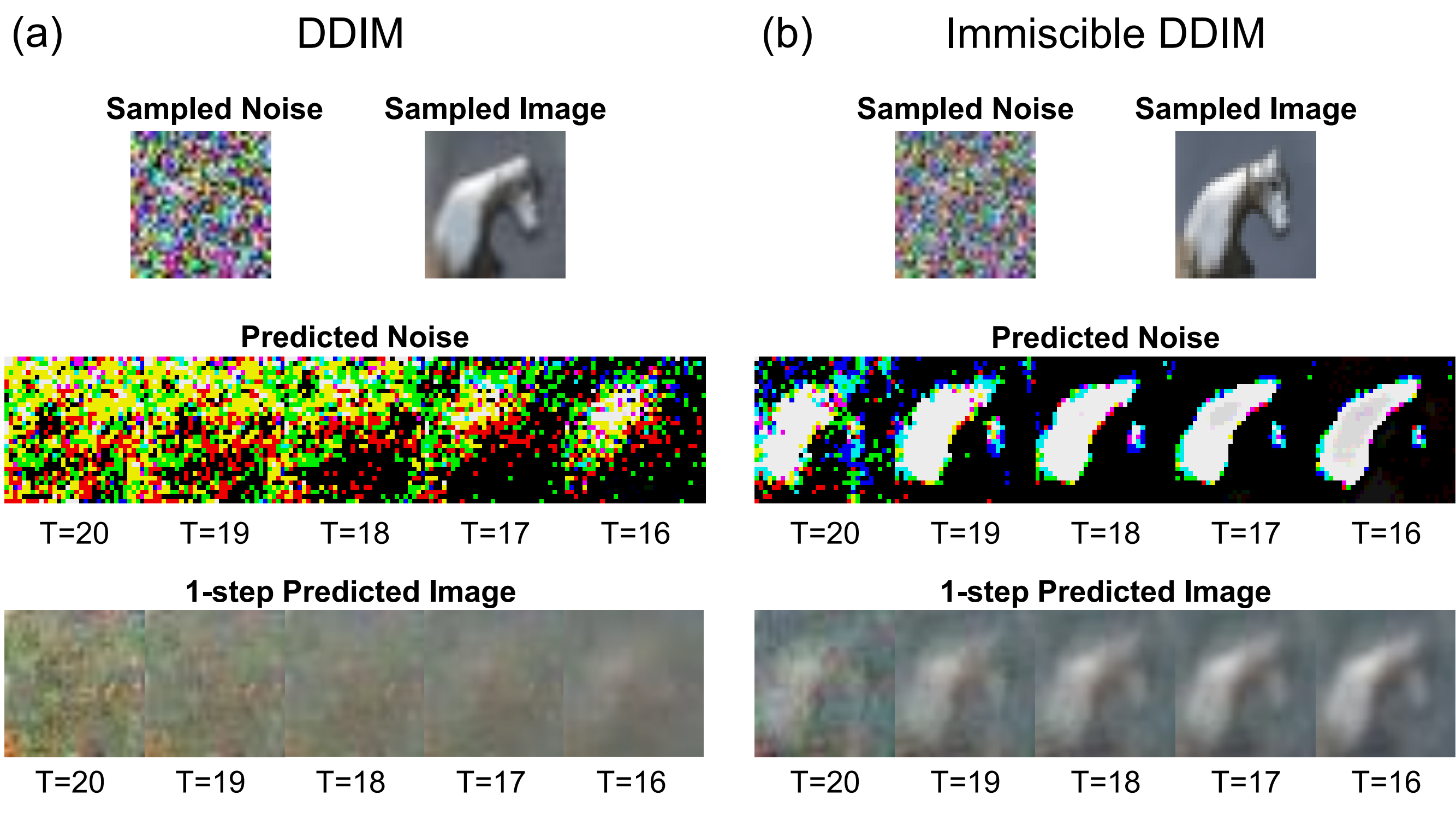
As shown in Fig. 3 (a), we study the predicted noises of different layers in a DDIM model with total inference steps of 20 to illustrate our discovery. Here $T=20$ means the layer of pure noise and $T=1$ is the final denoising layer outputing the generated image. We can see that the predicted noise for DDIM at $T=20$ does not provide much useful information, while subtracting this noise for the image does not provide any distinguishable image, which all support our hypothesis for the difficulty in denoising when $t$ is large. Similar observations are also shown in the concurrent work [42]. However, in our Immiscible Diffusion, while for each batch, we still have

$$p(\{x_{t}\}_{batch}\mid\{x_{0}\}_{batch})=\mathcal{N}(0,I),\quad and\quad p(x_{t})=\mathcal{N}(0,I),$$ (5)

for each specific $x_{t}$ or $x_{0}$, the conditional noise distribution does not follow the Gaussian distribution because of the batch-wise noise assignment

$$p(x_{t}\mid x_{0})\neq\mathcal{N}(0,I).$$ (6)

Instead of the Gaussian distribution, we assume that the predicted noise with noise assignment has a distribution described as follows

$$p(x_{t}\mid x_{0})=f(x_{t}-x_{0})\mathcal{N}(0,I),$$ (7)

where $f(x)$ is a function denoting the influence of assignment on the conditional distribution of $x_{t}$. Apparently, according to the definition of linear assignment problem [15], $f(x)$ decreases when $x$ increases its norm, specifically L2 norm as our default setting.

Therefore, from Equation 2 and 7, we have

$$\forall x_{0},x_{t},\quad p(x_{0}\mid x_{t})=f(x_{t}-x_{0})p(x_{0}),$$ (8)

which means that for a specific noise data-point, the possibility of denoising it to the nearby image data-point would be higher than to a far-away image.

For noise prediction task, we see that

$$\epsilon_{\theta}(x_{t},t)=\sum_{x_{0}}(ax_{0}-bx_{t})p(x_{0}\mid x_{t})=a\sum_{x_{0}}f(x_{t}-x_{0})x_{0}p(x_{0})-bx_{t}=a\overline{x_{0}f(x_{t}-x_{0})}-bx_{t}$$ (9)

where $\overline{x_{0}f(x_{t}-x_{0})}$ is the weighted average of $x_{0}$ with more weights on image data-points closer to the noisy data-point $x_{t}$ itself. Therefore, the noise predicted would lead to the average of nearby image data-points, which makes more senses than pointing to a constant. Indeed, in Fig. 3, we see that even for the pure noise layer, immiscible DDIM can predict noise effectively pointing to the shape of the horse image, and the 1-step prediction by substracting the predicted noise shows the outline of the horse correctly.

Note: The assignment problem has been extensively studied for decades [4, 16, 5]. In this paper, we use Hungarian algorithm [16] as our main assignment method. However, Hungarian matching has high complexity with $O(N^{3})$, which drastically slow down the training especially when we have high-dimensional image data (e.g., even using the mini image data $32\times 32\times 3=3072$). To mitigate this issue, we make a novel use of quantization for the image data and noise, i.e., we quantize the $fp32$ image and noise data to $fp16$ or $fp8$ to conduct the assignment, while keeping the same-precision input to diffusion models. This trick significantly reduces the overhead to a negligible level.

4 Experiments

4.1 Experiment Settings

To elaborate the performance of Immiscible Diffusion, we utilize the proposed method on Consistency Models [38], DDIM [36] and Stable Diffusion [32], and using CIFAR-10 [14], CelebA [21], tiny and random picked 10% ImageNet [3] datasets due to the limitation of computation resource. The training hyperparameters are shown in Tab. 1. Unspecified hyperparameters are taken the same as those in their baseline methods’ original papers. For evaluations, we compare the results generated by our Immiscible Diffusion method and the baseline using both qualitative assessments and the quantitative evaluation metric FID [7].

Note that for Consistency Models, we use the single step generation consistency training. For DDIM, we add no noise during sampling and use linear scheduling for picking sampling steps. For Stable Diffusion, we directly use the implementation from Diffusers of Huggingface team [31].

Table 1: Experiment setting.

Model	Consistency Model	DDIM	Consistency Model	Stable Diffusion Unconditional	Consistency Model	Stable Diffusion Class-conditional
Dataset	CIFAR-10	CIFAR-10	CelebA	10% ImageNet	Tiny ImageNet	ImageNet
Batch Size	512	256	1024	512	2048	2048
Resolution	$32\times 32$	$32\times 32$	$64\times 64$	$256\times 256$	$64\times 64$	$256\times 256$
Devices	$4\times A6000$	$1\times A5000$	$8\times A800$	$4\times A6000$	$16\times A800$	$8\times A800$

4.2 Main Results on Training Efficiency

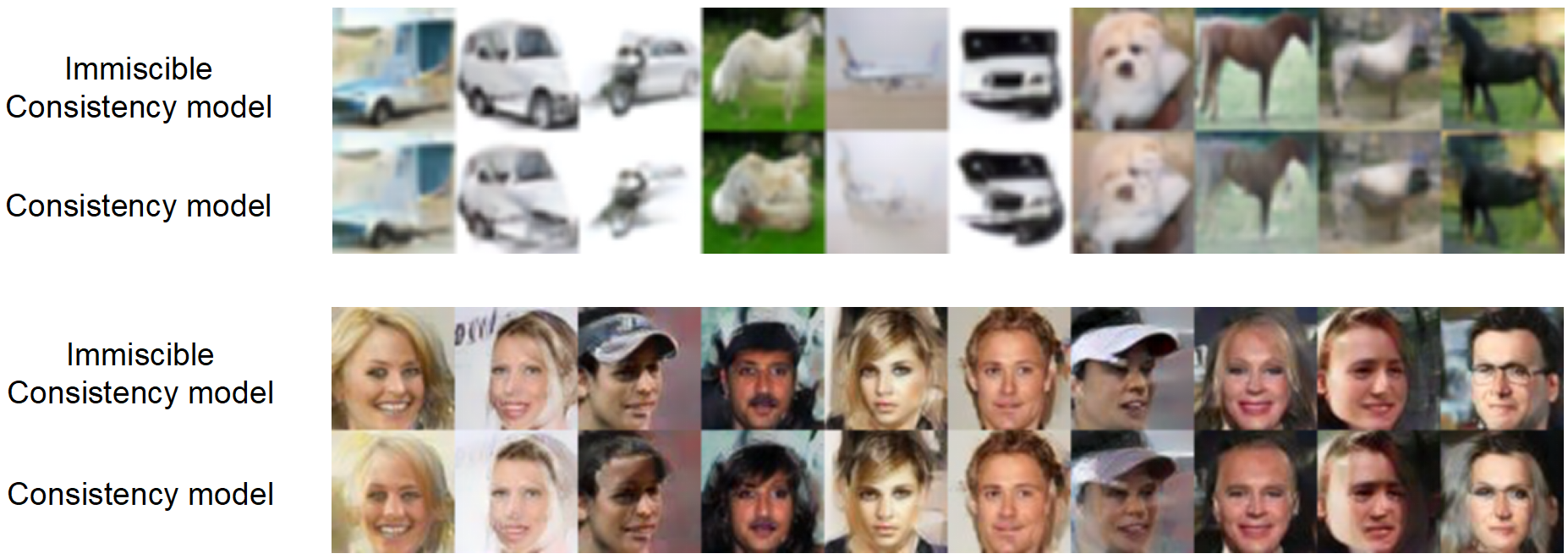
In Fig. 4, we show the FIDs of images generated with baseline and immiscible consistency models trained with different training steps on the CIFAR-10 dataset, the CelebA dataset and the tiny ImageNet dataset, respectively. We observe that the immiscible consistency model trains much faster than the baseline consistency model, and converges to a significantly lower FID on all of the CIFAR-10, CelebA, and tiny-ImageNet datasets. We also show the images generated by immiscible and baseline consistency models trained for 100k steps in Fig. 5, where we can see that the images generated by immiscible consistency model are much more complete and realistic. Tab. 2 further presents the training steps necessary to achieve specific reasonable FID thresholds. We find that the immiscible consistency model significantly improves the training efficiency by around 3x, proving the effectiveness of Immiscible Diffusion in training accelerations.

In the main experiment, we observe that our method on top of the Consistency Model is effective across the datasets varying from different data size and resolutions. Indeed, the Consistency Model is a few-step diffusion model, and our proposed Immiscible Diffusion especially works on improving the denoising effect when the noise level is high, as shown in Fig. 3. The improvement of the training efficiency on such a few step diffusion model further validates our findings.

One characteristic of the Consistency Model is that it approximates the SDE-diffusion model with ODE approximation. Thus the original image-noise mapping is highly jumbled together since it is highly possible that closed image data points are diffused to distant noise points. Our Immiscible Diffusion improves this issue by adjusting the trajectories of image-noise mapping and making them more distinguishable.

Figure 4: Evaluation of baseline and immiscible consistency models on CIFAR-10, CelebA, and tiny-ImageNet dataset. We illustrate the FID of two models with different training steps. Clearly, immiscible consistency models have much higher efficiency than the traditional one.

Table 2: Immiscible Diffusion boosts training efficiency for consistency model on CIFAR-10 dataset.

FID threshold 12.00 11.00 10.00 Training Steps (k) for Baseline Consistency Model 290 450 >800 Training Steps (k) for Immiscible Consistency Model 110 140 190

Figure 5: Qualitative comparison for immiscible and baseline consistency model. We show images generated with the two models trained for 100k steps respectively. Compared to baseline method, immiscible models can catch more details and more feature of objects.

More baselines: To show the generalization of Immiscible Diffusion for more baselines, we further conduct experiments on two baselines: DDIM [36] and Stable Diffusion [30] on the CIFAR-10 and the randomly picked 10% ImageNet dataset, respectively. As shown in Fig. 6, we find that our immiscible DDIM significantly improves the training speed and the FID compared to those of the baseline DDIM on the CIFAR-10 dataset. This improvement demonstrates the effectiveness of our proposed method works beyond the Consistency Model and can be generalized to more few-step denoising models.

Figure 6: Evaluation of baseline and immiscible DDIM on CIFAR-10 dataset, using 20 inference steps. (a) FID of two models with different training steps (b) Qualitative comparison of two models trained 100k steps.

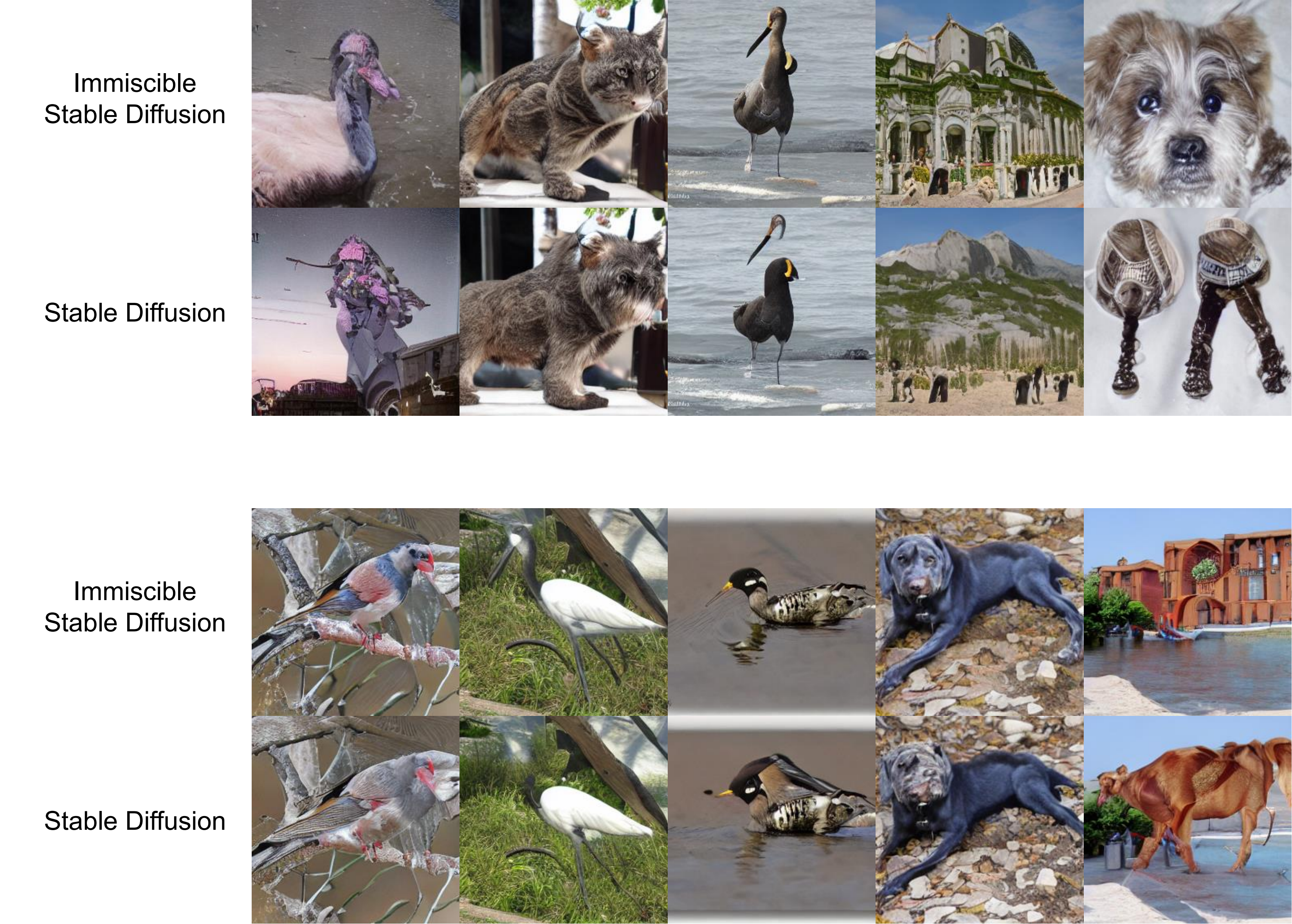
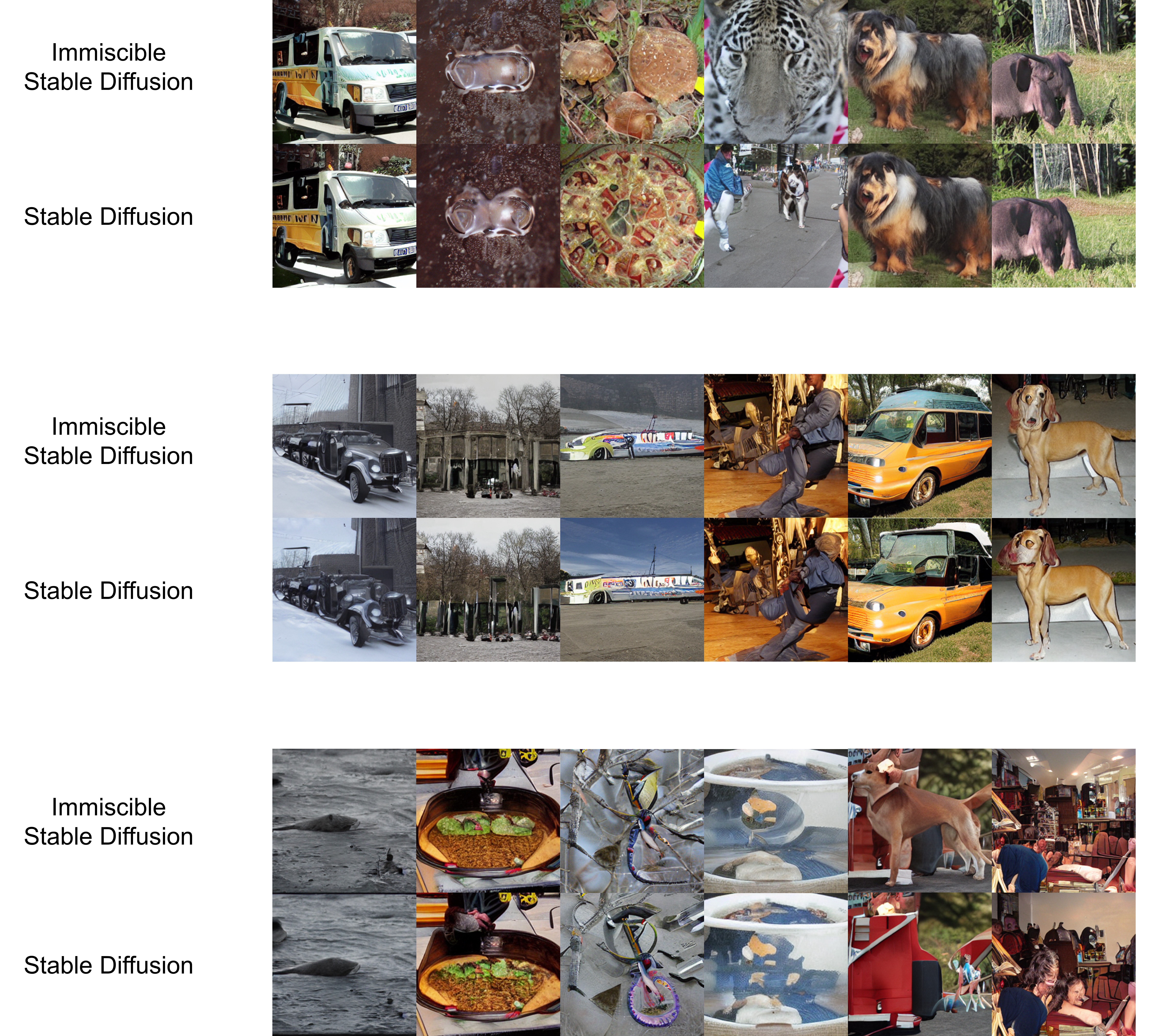
To further evaluate the generalizability on the popular baseline, Stable Diffusion [30], we conduct experiments on the ImageNet dataset. We observe that immiscible Stable Diffusion and baseline Stable Diffusion achieve similar FID without significant gap, yet our immiscible Stable Diffusion is able to generate much higher quality images from a subjective human judgement. For example, Fig. 7 shows our proposed method generates significantly clearer images compared to the baseline. More visualization without any cherry-picking can be seen in the supplementary materials. We indicate that even though FID is the primary metric and remarkably successful, the metric is known to sometimes disagree with human judgement [17].

Class-conditional Generation: We extend immiscible diffusions to class-conditional generations on ImageNet dataset with Stable Diffusion [32], to explore the performance of immiscible diffusion in conditional cases. Results are shown in Fig. 8, where we observe that the FID for immiscible class-conditional Stable Diffusion is 20.90, which is 1.53 lower than our Stable Diffusion baseline. Qualitative comparisons further prove such performance enhancements, which augment the effectiveness of immiscible diffusions into more commonly-used conditional generations.

Figure 7: Images generated by immiscible and baseline Stable Diffusion trained on ImageNet for 70k steps. We see that the immiscible Stable Diffusion presents more reasonable modal and catch more general features and details.

4.3 Discussion

To further understand the proposed Immiscible Diffusion method, we delve into several key questions to ablate our approach:

Figure 8: Evaluation of baseline and immiscible class-conditional Stable Diffusion on ImageNet dataset, using 20 inference steps. (a) FID of two models with different training steps (b) Qualitative comparison of two models trained 20k steps.

How much does image-noise distance reduce in the assignment? Tab. 3 shows the reduction in distance after the image-noise assignment. We find that the distance only reduces by about 2%, with a slight increase observed at higher batch sizes. However, this small change in distance is sufficient to effectively activate the denoising at high-noise levels, significantly boosting training efficiency. We attribute the low distance reduction rate after the assignment to the extremely high dimensionality (3072 for each image of the CIFAR-10 dataset) of the image and noise space. Furthermore, we indicate that our assignment method does not introduce significant extra overhead due to our utilization of quantized assignment in our practical implementation. Even for a large per-GPU batch size of 1024, our algorithm only brings in additional 22.8ms, demonstrating the potential of utilization for future applications.

Table 3: Image-noise datapoint L2 distance reduction after the assignment for minimizing it.

Batch Size	128	256	512	1024
$\Delta$Dist.	-1.93%	-2.16%	-2.32%	-2.44%
Assignment Time (ms)	5.4	6.7	8.8	22.8

Which distance function should be used for assignment? We use the L2 norm for our experiments. However, we note that the L2 norm may face more challenges in distance evaluation in high-dimensional spaces compared to the L1 norm. Therefore, we compare the performance of immiscible DDIMs using assignments based on the L1 and L2 norms. The results, as illustrated in Tab. 4, show that using the L2 norm provides better performance than the L1 norm.

Table 4: FID of using L1 or L2 norm for noise assginment in immiscible DDIM on CIFAR-10.

Traning Steps (k)	70.2	93.6	117.0	140.4	163.8
DDIM	6.30	5.56	4.86	4.34	4.12
Immiscible DDIM using L2 Norm	5.28	4.56	4.13	3.81	3.70
Immiscible DDIM using L1 Norm	5.34	4.66	4.16	3.87	3.82

How does Immiscible Diffusion work for different inference steps in DDIM? As we improve the utilization of high (noisy) diffusion steps, our performance improves, particularly when there are not too many redundant denoising layers. Specifically, we observe more significant performance boosts with immiscible DDIM when the number of inference denoising steps is lower, as shown in Tab. 5.

Table 5: FID improvements of Immiscible DDIM with different inference steps

Inference Steps	1000	500	100	50	20
FID with baseline DDIM	3.82	3.91	5.2	6.63	10.03
FID with Immiscible DDIM	3.67	3.74	4.32	5.14	7.46
$\Delta$FID	-0.15	-0.17	-0.98	-1.49	-2.57

5 Conclusion, Limitations, and Future Work

Inspired by the immiscible phenomenon in physics, we introduce Immiscible Diffusion, a method to improve noise-data mapping to accelerate diffusion training. Specifically, Immiscible Diffusion is an assignment-then-diffusion strategy. It minimizes the image-noise pair distance within a mini-batch so that the similar images are diffused to nearby noise points. This simple approach requires only one line of code and includes a quantized-assignment strategy to reduce computational overhead. Experiments show our Immiscible Diffusion approach speeds up training by approximately 3x on the CIFAR-10 dataset, 1.3x on the CelebA dataset, and 1.2x on the tiny-ImageNet dataset. Thus, we show that Immiscible Diffusion can generalize to across datasets and different baselines. Further analysis is provided to explain how this works.

Limitation. Our current assignment strategy is straightforward and not necessarily optimal. Due to the limited computational resources, our experiments are mainly conducted on small-scale datasets, so we lack the validation on larger-scale dataset such as LAION. In future work, we will improve the assignment strategy to cater to practical utilization of conditional generation such as accelerating the text-to-image or text-to-video diffusion training.

Broader impact. With the increased use of diffusion models for image and video generation, the training of diffusion models is certain to become an increasing portion of data center workloads. Moreover, training time is significant bottleneck to model development. Our proposed method significantly improves the efficiency of diffusion model training. We believe our method has the potential to accelerate progress and to reduce the cost of development in this field.

Appendix A Supplemental material

A.1 Generated images from immiscible and baseline stable diffusion models trained on 10% ImageNet Dataset for 70k steps without cherry-picking

Figure 9: Generated images from immiscible and baseline stable diffusion models trained on 10% ImageNet Dataset for 70k steps without cherry-picking

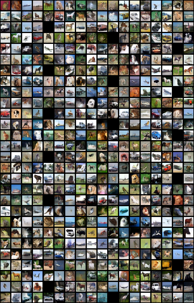
A.2 Generated images from immiscible and baseline consistency models trained on CIFAR-10 Dataset for 100k steps without cherry-picking

Figure 10: Generated images from baseline consistency models trained on CIFAR-10 Dataset for 100k steps without cherry-picking.

Figure 11: Generated images from immiscible consistency models trained on CIFAR-10 Dataset for 100k steps without cherry-picking.

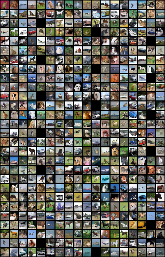
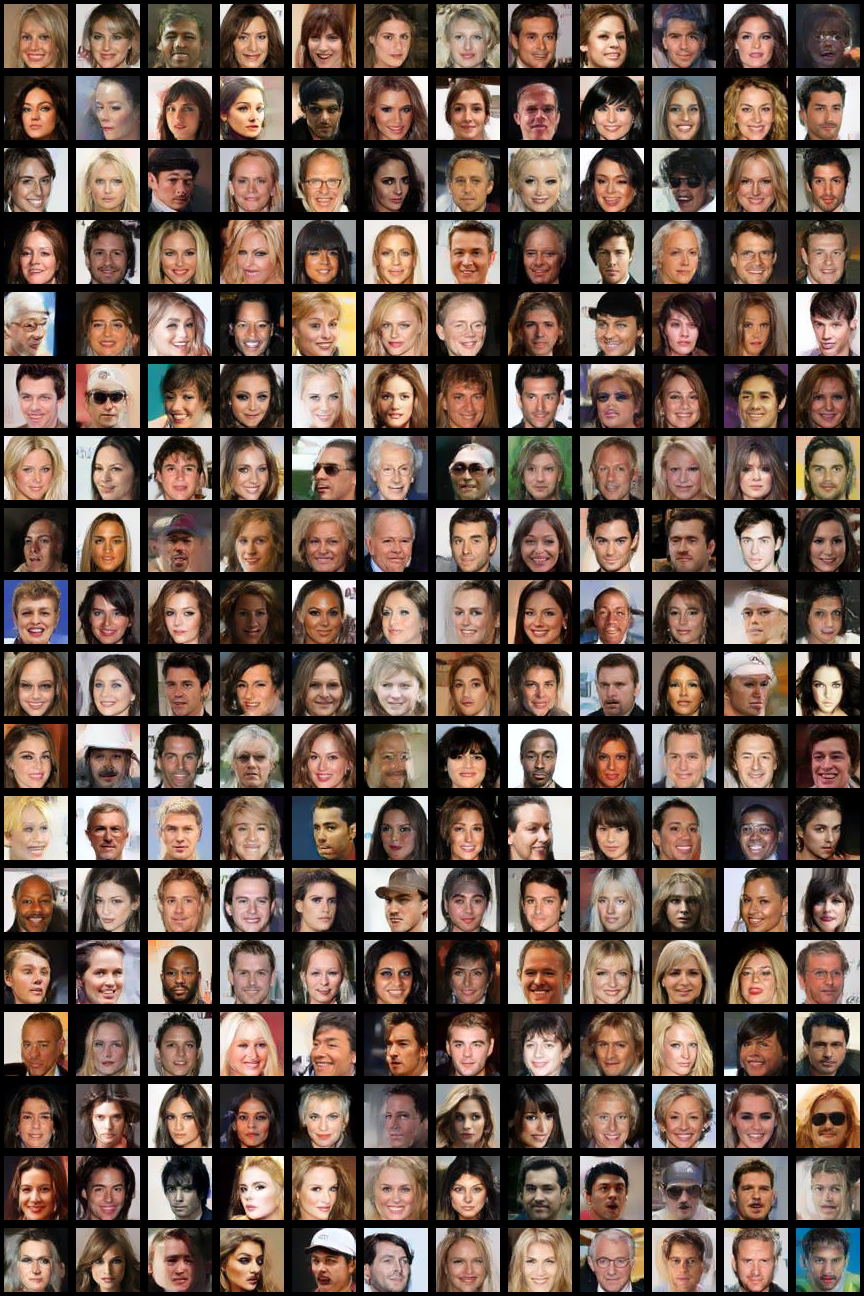
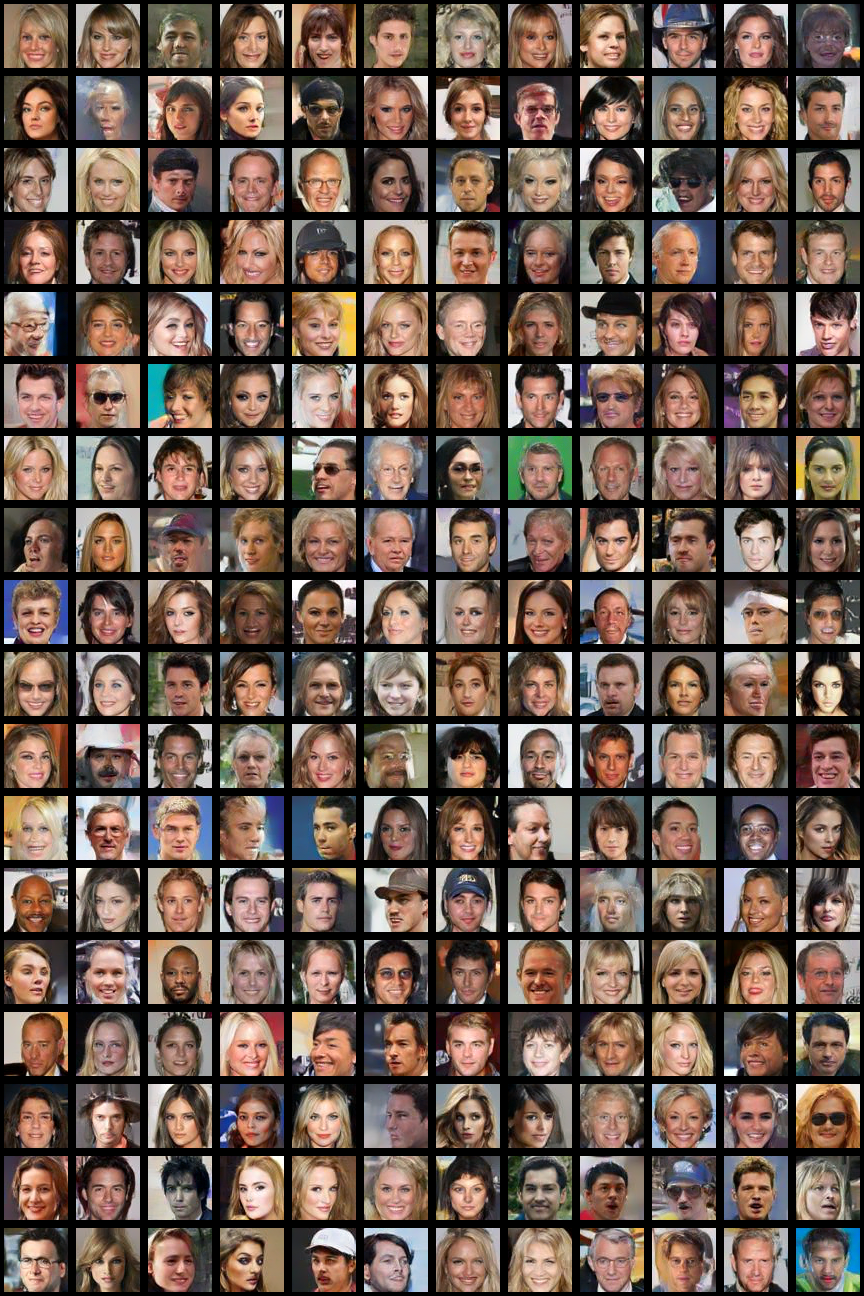
A.3 Generated images from immiscible and baseline consistency models trained on CelebA Dataset for 100k steps without cherry-picking

Figure 12: Generated images from baseline consistency models trained on CelebA Dataset for 100k steps without cherry-picking.

Figure 13: Generated images from immiscible consistency models trained on CelebA Dataset for 100k steps without cherry-picking.

References

- [1] Kevin Black, Mitsuhiko Nakamoto, Pranav Atreya, Homer Walke, Chelsea Finn, Aviral Kumar, and Sergey Levine. Zero-shot robotic manipulation with pretrained image-editing diffusion models. arXiv preprint arXiv:2310.10639, 2023.
- [2] Cheng Chi, Siyuan Feng, Yilun Du, Zhenjia Xu, Eric Cousineau, Benjamin Burchfiel, and Shuran Song. Diffusion policy: Visuomotor policy learning via action diffusion. arXiv preprint arXiv:2303.04137, 2023.
- [3] Jia Deng, Wei Dong, Richard Socher, Li-Jia Li, Kai Li, and Li Fei-Fei. Imagenet: A large-scale hierarchical image database. In 2009 IEEE conference on computer vision and pattern recognition, pages 248–255. Ieee, 2009.
- [4] Lawrence W Dowdy and Derrell V Foster. Comparative models of the file assignment problem. ACM Computing Surveys (CSUR), 14(2):287–313, 1982.
- [5] Paul C Gilmore. Optimal and suboptimal algorithms for the quadratic assignment problem. Journal of the society for industrial and applied mathematics, 10(2):305–313, 1962.
- [6] Ian Goodfellow, Jean Pouget-Abadie, Mehdi Mirza, Bing Xu, David Warde-Farley, Sherjil Ozair, Aaron Courville, and Yoshua Bengio. Generative adversarial nets. Advances in neural information processing systems, 27, 2014.
- [7] Martin Heusel, Hubert Ramsauer, Thomas Unterthiner, Bernhard Nessler, and Sepp Hochreiter. Gans trained by a two time-scale update rule converge to a local nash equilibrium, 2018.
- [8] Jonathan Ho, William Chan, Chitwan Saharia, Jay Whang, Ruiqi Gao, Alexey Gritsenko, Diederik P Kingma, Ben Poole, Mohammad Norouzi, David J Fleet, et al. Imagen video: High definition video generation with diffusion models. arXiv preprint arXiv:2210.02303, 2022.
- [9] Jonathan Ho, Ajay Jain, and Pieter Abbeel. Denoising diffusion probabilistic models. Advances in neural information processing systems, 33:6840–6851, 2020.
- [10] Jonathan Ho, Tim Salimans, Alexey Gritsenko, William Chan, Mohammad Norouzi, and David J Fleet. Video diffusion models. Advances in Neural Information Processing Systems, 35:8633–8646, 2022.
- [11] Tero Karras, Miika Aittala, Jaakko Lehtinen, Janne Hellsten, Timo Aila, and Samuli Laine. Analyzing and improving the training dynamics of diffusion models. arXiv preprint arXiv:2312.02696, 2023.
- [12] Dongjun Kim, Chieh-Hsin Lai, Wei-Hsiang Liao, Naoki Murata, Yuhta Takida, Toshimitsu Uesaka, Yutong He, Yuki Mitsufuji, and Stefano Ermon. Consistency trajectory models: Learning probability flow ode trajectory of diffusion. arXiv preprint arXiv:2310.02279, 2023.
- [13] Akio Kodaira, Chenfeng Xu, Toshiki Hazama, Takanori Yoshimoto, Kohei Ohno, Shogo Mitsuhori, Soichi Sugano, Hanying Cho, Zhijian Liu, and Kurt Keutzer. Streamdiffusion: A pipeline-level solution for real-time interactive generation. arXiv preprint arXiv:2312.12491, 2023.
- [14] Alex Krizhevsky, Geoffrey Hinton, et al. Learning multiple layers of features from tiny images. Toronto, ON, Canada, 2009.
- [15] H. W. Kuhn. The hungarian method for the assignment problem. Naval Research Logistics Quarterly, 2(1-2):83–97, 1955.
- [16] Harold W Kuhn. The hungarian method for the assignment problem. Naval research logistics quarterly, 2(1-2):83–97, 1955.
- [17] Tuomas Kynkäänniemi, Tero Karras, Miika Aittala, Timo Aila, and Jaakko Lehtinen. The role of imagenet classes in fr’echet inception distance. arXiv preprint arXiv:2203.06026, 2022.
- [18] Muyang Li, Ji Lin, Chenlin Meng, Stefano Ermon, Song Han, and Jun-Yan Zhu. Efficient spatially sparse inference for conditional gans and diffusion models, 2023.
- [19] Xiuyu Li, Yijiang Liu, Long Lian, Huanrui Yang, Zhen Dong, Daniel Kang, Shanghang Zhang, and Kurt Keutzer. Q-diffusion: Quantizing diffusion models. In Proceedings of the IEEE/CVF International Conference on Computer Vision (ICCV), pages 17535–17545, October 2023.
- [20] Xingchao Liu, Xiwen Zhang, Jianzhu Ma, Jian Peng, et al. Instaflow: One step is enough for high-quality diffusion-based text-to-image generation. In The Twelfth International Conference on Learning Representations, 2023.
- [21] Ziwei Liu, Ping Luo, Xiaogang Wang, and Xiaoou Tang. Deep learning face attributes in the wild. In Proceedings of the IEEE international conference on computer vision, pages 3730–3738, 2015.
- [22] Cheng Lu, Yuhao Zhou, Fan Bao, Jianfei Chen, Chongxuan Li, and Jun Zhu. Dpm-solver: A fast ode solver for diffusion probabilistic model sampling in around 10 steps. Advances in Neural Information Processing Systems, 35:5775–5787, 2022.
- [23] Cheng Lu, Yuhao Zhou, Fan Bao, Jianfei Chen, Chongxuan Li, and Jun Zhu. Dpm-solver++: Fast solver for guided sampling of diffusion probabilistic models. arXiv preprint arXiv:2211.01095, 2022.
- [24] Grace Luo, Lisa Dunlap, Dong Huk Park, Aleksander Holynski, and Trevor Darrell. Diffusion hyperfeatures: Searching through time and space for semantic correspondence. Advances in Neural Information Processing Systems, 36, 2024.
- [25] Simian Luo, Yiqin Tan, Longbo Huang, Jian Li, and Hang Zhao. Latent consistency models: Synthesizing high-resolution images with few-step inference, 2023.
- [26] OpenAI. https://openai.com/sora, 2024.
- [27] William Peebles and Saining Xie. Scalable diffusion models with transformers. arXiv preprint arXiv:2212.09748, 2022.
- [28] Aaditya Prasad, Kevin Lin, Jimmy Wu, Linqi Zhou, and Jeannette Bohg. Consistency policy: Accelerated visuomotor policies via consistency distillation, 2024.
- [29] Yuxi Ren, Xin Xia, Yanzuo Lu, Jiacheng Zhang, Jie Wu, Pan Xie, Xing Wang, and Xuefeng Xiao. Hyper-sd: Trajectory segmented consistency model for efficient image synthesis, 2024.
- [30] Robin Rombach, Andreas Blattmann, Dominik Lorenz, Patrick Esser, and Björn Ommer. High-resolution image synthesis with latent diffusion models. In Proceedings of the IEEE/CVF conference on computer vision and pattern recognition, pages 10684–10695, 2022.
- [31] Robin Rombach, Andreas Blattmann, Dominik Lorenz, Patrick Esser, and Björn Ommer. High-resolution image synthesis with latent diffusion models. In Proceedings of the IEEE/CVF Conference on Computer Vision and Pattern Recognition (CVPR), pages 10684–10695, June 2022.
- [32] Robin Rombach, Andreas Blattmann, Dominik Lorenz, Patrick Esser, and Björn Ommer. High-resolution image synthesis with latent diffusion models, 2021.
- [33] Axel Sauer, Dominik Lorenz, Andreas Blattmann, and Robin Rombach. Adversarial diffusion distillation. arXiv preprint arXiv:2311.17042, 2023.
- [34] Jascha Sohl-Dickstein, Eric A. Weiss, Niru Maheswaranathan, and Surya Ganguli. Deep unsupervised learning using nonequilibrium thermodynamics, 2015.
- [35] Jiaming Song, Chenlin Meng, and Stefano Ermon. Denoising diffusion implicit models. arXiv preprint arXiv:2010.02502, 2020.
- [36] Jiaming Song, Chenlin Meng, and Stefano Ermon. Denoising diffusion implicit models. In International Conference on Learning Representations, 2021.
- [37] Yang Song and Prafulla Dhariwal. Improved techniques for training consistency models. arXiv preprint arXiv:2310.14189, 2023.
- [38] Yang Song, Prafulla Dhariwal, Mark Chen, and Ilya Sutskever. Consistency models, 2023.
- [39] Yang Song, Jascha Sohl-Dickstein, Diederik P Kingma, Abhishek Kumar, Stefano Ermon, and Ben Poole. Score-based generative modeling through stochastic differential equations. arXiv preprint arXiv:2011.13456, 2020.
- [40] Luming Tang, Menglin Jia, Qianqian Wang, Cheng Perng Phoo, and Bharath Hariharan. Emergent correspondence from image diffusion. Advances in Neural Information Processing Systems, 36:1363–1389, 2023.
- [41] Pauli Virtanen, Ralf Gommers, Travis E. Oliphant, Matt Haberland, Tyler Reddy, David Cournapeau, Evgeni Burovski, Pearu Peterson, Warren Weckesser, Jonathan Bright, Stéfan J. van der Walt, Matthew Brett, Joshua Wilson, K. Jarrod Millman, Nikolay Mayorov, Andrew R. J. Nelson, Eric Jones, Robert Kern, Eric Larson, C J Carey, İlhan Polat, Yu Feng, Eric W. Moore, Jake VanderPlas, Denis Laxalde, Josef Perktold, Robert Cimrman, Ian Henriksen, E. A. Quintero, Charles R. Harris, Anne M. Archibald, Antônio H. Ribeiro, Fabian Pedregosa, Paul van Mulbregt, Aditya Vijaykumar, Alessandro Pietro Bardelli, Alex Rothberg, Andreas Hilboll, Andreas Kloeckner, Anthony Scopatz, Antony Lee, Ariel Rokem, C. Nathan Woods, Chad Fulton, Charles Masson, Christian Häggström, Clark Fitzgerald, David A. Nicholson, David R. Hagen, Dmitrii V. Pasechnik, Emanuele Olivetti, Eric Martin, Eric Wieser, Fabrice Silva, Felix Lenders, Florian Wilhelm, G. Young, Gavin A. Price, Gert-Ludwig Ingold, Gregory E. Allen, Gregory R. Lee, Hervé Audren, Irvin Probst, Jörg P. Dietrich, Jacob Silterra, James T Webber, Janko Slavič, Joel Nothman, Johannes Buchner, Johannes Kulick, Johannes L. Schönberger, José Vinícius de Miranda Cardoso, Joscha Reimer, Joseph Harrington, Juan Luis Cano Rodríguez, Juan Nunez-Iglesias, Justin Kuczynski, Kevin Tritz, Martin Thoma, Matthew Newville, Matthias Kümmerer, Maximilian Bolingbroke, Michael Tartre, Mikhail Pak, Nathaniel J. Smith, Nikolai Nowaczyk, Nikolay Shebanov, Oleksandr Pavlyk, Per A. Brodtkorb, Perry Lee, Robert T. McGibbon, Roman Feldbauer, Sam Lewis, Sam Tygier, Scott Sievert, Sebastiano Vigna, Stefan Peterson, Surhud More, Tadeusz Pudlik, Takuya Oshima, Thomas J. Pingel, Thomas P. Robitaille, Thomas Spura, Thouis R. Jones, Tim Cera, Tim Leslie, Tiziano Zito, Tom Krauss, Utkarsh Upadhyay, Yaroslav O. Halchenko, and Yoshiki Vázquez-Baeza. Scipy 1.0: fundamental algorithms for scientific computing in python. Nature Methods, 17(3):261–272, February 2020.
- [42] Kai Wang, Yukun Zhou, Mingjia Shi, Zhihang Yuan, Yuzhang Shang, Xiaojiang Peng, Hanwang Zhang, and Yang You. A closer look at time steps is worthy of triple speed-up for diffusion model training, 2024.
- [43] Zhendong Wang, Yifan Jiang, Huangjie Zheng, Peihao Wang, Pengcheng He, Zhangyang Wang, Weizhu Chen, and Mingyuan Zhou. Patch diffusion: Faster and more data-efficient training of diffusion models. arXiv preprint arXiv:2304.12526, 2023.
- [44] Chenfeng Xu, Huan Ling, Sanja Fidler, and Or Litany. 3difftection: 3d object detection with geometry-aware diffusion features, 2023.