Faithful Density-Peaks Clustering via Matrix Computations on MPI Parallelization System
Abstract
Density peaks clustering (DP) has the ability of detecting clusters of arbitrary shape and clustering non-Euclidean space data, but its quadratic complexity in both computing and storage makes it difficult to scale for big data. Various approaches have been proposed in this regard, including MapReduce based distribution computing, multi-core parallelism, presentation transformation (e.g., d-tree, Z-value), granular computing, and so forth. However, most of these existing methods face two limitations. One is their target datasets are mostly constrained to be in Euclidian space, the other is they emphasize only on local neighbors while ignoring global data distribution due to restriction to cut-off kernel when computing density. To address the two issues, we present a faithful and parallel DP method that makes use of two types of vector-like distance matrices and an inverse leading-node-finding policy. The method is implemented on a message passing interface (MPI) system. Extensive experiments showed that our method is capable of clustering non-Euclidean data such as in community detection, while outperforming the state-of-the-art counterpart methods in accuracy when clustering large Euclidean data. Our code is publicly available at https://github.com/alanxuji/FaithPDP.
1 Introduction
As a fundamental technique to depict the data distribution unsupervisedly, clustering relates closely to various subfields of machine learning such as semi-supervised transductive learning zhou2007spectral , fu2015transductive , contrastive learning li2021contrastive , sharma2020clustering , domain-adaption deng2021joint , liang2019aggregating , and so on. In these fields, the similarity of data within a cluster is very helpful for promoting the efficiency and accuracy of a given learning model. Clustering itself can be used directly in many applications as well, for example, in image segmentation coleman1979image , dong2005color , tang2020fuzzy , community discovery wang2014neiwalk , niu2023overlapping and recommendation system farseev2017cross , cui2020personalized . There have been many clustering methods, among which density-peak clustering (DP) rodriguez2014clustering is very successful and influential due to its ability to detect clusters of arbitrary shapes and non-iterative computing procedure.
However, there is a bottleneck in the original DP, that is, it requires complexity to compute and store the distance matrix, which prevent DP from directly scaling for big data analytics. Many excellent research works have been put-forward to address this issue that can be categorized into three streams: a) utilizing data structure (utilizing a data-structure amagata2023efficient or data encoding lu2022distributed ), b) modifying computing architecture (Map-reduce distributed or multi-core parallelism) zhang2016efficient , amagata2021fast , and c) employing new computing methodology (e.g., granular computing) cheng2023fast . For the data structure category,
These methods effectively endow DP the ability to process large scale data, but leave two main issues unaddressed. The first is because of relying on data organization, approximate encoding, or data splitting and merging, they lost the ability of capturing the local sophisticated structure and global data distribution (which is the first core advantage of DP). Fig. 3 provides an illustrative example. The second is that most of them typically constrained their target data to lie in Euclidean space, and lost the ability of taking a distance as input to perform clustering (which is the second core advantage of DP).
To solve the aforementioned weaknesses of the existing methods that scales DP, we propose in this paper a faithful parallel DP (FaithPDP) that achieves the identical intermediate results and final clustering result to original plain DP, while keeping the memory consumption linear to data size. Because the provable faithfulness of the proposed parallelism of DP, FaithPDP keeps the two core advantages of vanilla DP, that is, it can capture the micro subtle structure of data thus achieves high accuracy and it has the ability to clustering non-Euclidean data (e.g., clustering nodes in a social network). The contributions of our method include three aspects:
-
1.
The proposed method reduced the computing time and memory occupation to enable DP to clustering big data with the intermediate results and final result being identical to original DP. Our method achieves pseudo-linear time complexity and linear space complexity.
-
2.
FaithPDP keeps the same ability to cluster non-Euclidean data (e.g., social network node cluster) as vanilla DP, while being able to accommodate large scale data.
-
3.
Theoretical analysis and extensive experiments through massage passing interface (MPI) nielsen2016introduction show that our method achieves superior accuracy while keeping competitive efficiency when dealing with either Euclidean or graph data.
2 Related Works
There have been a number of works aiming to scale DP to cluster massive data, which can be categorized as exact and approximate. By “exact", it means the method can generate exactly the same intermediate and final results as DP with integer cut-off kernel, rather than with Gaussian kernel that leads to real density.
2.1 Exact Methods
Data structure. Ex-DPC amagata2023efficient employs kd-tree structure to facilitate fast computing of local density and depending distance . All methods based on kd-tree use cut-off kernel to compute density, which causes integer density and subsequent random sorting of the objects with the same density. Besides, they calculate the position of each data point through iterative partitioning on each dimension, thus prefer data with low dimensionality.
Computing architecture. The earliest effort to scaling DP for big data is taken by Zhang et. al. zhang2016efficient introducing MapReduce framework to distributedly clustering data. In their paper, locality sensitive hash (LSH) is utilized to avoid high communication and computation overload of Basic-DDP. Later, multi-core based parallelization is introduce to accelerate DP amagata2021fast , which is the pioneering work based on kd-tree and recently improved and consummated as in amagata2023efficient .
2.2 Approximate Methods
Ex-DPC++ amagata2023efficient uses kd-tree and cover-tree (another data structure to accelerate nearest neighbor query in any metric space) beygelzimer2006cover , to expand the application scenario of Ex-DPC. CFSFDP+A uses a k-means clustering to obtain an initial partition of the data, and reduces the workload of computation of density and -distance (called separation therein) based on the partition bai2017fast . Similarly, GB-DP cheng2023fast employs k-means (usually k is set to be 2) to construct granular balls, and perform DP clustering based on the granular balls rather than original data points, hence achieve considerable acceleration in computing.
3 Preliminaries
Density Peaks Clustering (DP). DP consists of three major steps, aiming to compute four key vectors (namely, local density , depending node , depending distance , and center potential ) based on the pair-wise distance matrix . It dose not matter whether is computed from a dataset in Euclidean space or from a graph . The goal is to assign a cluster label to ecah or a node in graph . We use to denote all the clustering labels and the set of centers. DP consists of three steps as follows.
(1) Local density , where .
(2) Depending node and depending distance 111These also named dependent points and dependent distance in amagata2023efficient . In addition, they are also named as leading node and -distance in xu2016denpehc , where and .
(3) Center potential , where denotes Hadamard product.
The clustering process is accomplished by adaptive selecting the centers featured with extraordinarily large elements in and assign the rest of the data points to each cluster according to a chain rule, i.e.,
| (1) |
Accelerating DP via matrix computing. Matrix based computation of has been proposed to replace the pair-wise distance computation, for either Euclidean distance or cosine similarity as in Eq. (2)
| (2) |
or Eq. (3) xu2021lapoleaf
| (3) |
where is a subset of (or the embedding of nodes in graph ) consists of samples in the form of row vector, and are the operators of element-wise square and element-wise division, respectively. We omit the superscript or afterwards and denote as for short. We use Euclidean distance as default unless specified otherwise. Consequently, the local density vector segments of a subset samples can be computed as in Eq. (4),
| (4) |
in which all the elements in matrix are first divided by , then take Hadamard square and Hadamard exponential. Finally, the elements in each row are summed to get the local density of corresponding sample.
Parallelism via Message-Passing Interface. Message Passing Interface (MPI) is a standardized and portable message-passing system designed to implement parallel computing, which is established since 1994 and still under active updating nowadays mpi41 . The basic functions of MPI that facilitate parallel computing include message sending/receiving, gathering/broadcasting, and so forth. Early MPI supports mainstream programming languages (such as C/C++, Fortran), and later MPI for Python was developed dalcin2005mpi ; dalcin2021mpi4py . For efficiency of development, we choose MPI4py in our implementation.
4 Faithful Parallel DPC
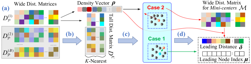
To make our method easier to follow, we depict our computing flowchart in Fig. 1 and first describe our method of sequential version in Algorithm 1, then a final faithful parallel DP (FaithPDP) is described in Algorithm .
Algorithm 2 described the faithful and parallel DP based on MPI system.
5 Experiments
All the experiments are conducted on two Dell T7920 workstations 222Each equipped with two Xeon 6230R CPUs, 64G DDR4 Memory, an NVIDIA GForce 3090 GPU, 512G SSD + 4T HDD Hard Disk., Python 3.9 and mpi4py 3.1.5 running in a Conda virtual environment configured on the operating system of Ubuntu 22.04.
5.1 Design purpose
Our experiment is designed to answer the following questions.
Q1: What the difference between FaithPDP and the existing scaling-up methods of DP?
Q2: How is the performance improvement of FaithPDP over other competing models on learned representation of real data?
Q3: How does FaithPDP perform on high-dimensional Euclidean data?
Q4: Is FaithPDP perform efficiently while being accurate?
5.2 Datasets and baseline models
To answer the research questions Q1~Q5, the chosen datasets vary from medium scale to huge scale, from Euclidean to graph, from synthetic to real, and from low-dimensional to high-dimensional. The information of the datasets used in our empirical evaluations is listed in Table 1.
| SN | Dataset | Type | Source | Data size † | # Clusters | Purpose |
|---|---|---|---|---|---|---|
| DS1 | 5Spriral50k | Euclidean | Synthetic | (52,834; 2) | 5 | Q1 |
| DS2 | 5Spiral500k | Euclidean | Synthetic | (528,320; 2) | 5 | Q1, Q4 |
| DS3 | Pamap2_sub1 | Euclidean | Real | (7,528; 8,109) | 15 | Q2, Q3 |
| DS4 | Opportunity_s2ADL3 | Euclidean | Real | (34,232; 243) | 4 | Q2, Q3 |
| DS5 | MINIST159 | Euclidean | Real | (18,112; 784) | 3 | Q2, Q3 |
| DS6 | MINIST159_emb | Euclidean | Real | (18,112; 2) | 3 | Q2 |
| DS7 | MINIST_tr | Euclidean | Real | (60,000; 784) | 10 | Q1, Q3 |
| DS8 | Email_emb | Euclidean | Real | (1,005; 64) | 41 | Q2 |
-
1
: (; ) denotes the number of samples and dimensions and <; > the number of nodes and edges.
We evaluated our FaithPDP against six state-of-the-art methods. They are
1) Index-List rasool2022index : a method that construct a list of nearest neighbors for fast density computing;
2) RN-List: an approximate alternative of Index-List;
3) GB-DP cheng2023fast : changes the clustering objects from finest-grained data points to granular balls built with hierarchical k-means splitting;
4) Ex-DPC amagata2021fast ; amagata2023efficient : fast density and leading point computation by restricting search field in a kd-tree;
5) Z-Value lu2022distributed : fast DP through encoding the samples into a integer space;
6) Ex-DPC++ amagata2023efficient : Improve Ex-DPC further with another data structure named cover-tree.
5.3 Performance comparison and discussion
Performance on accuracy. The accuracy is evaluated under the metrics of normalized mutual information (NMI) strehl2002cluster and adjusted Rand index (ARI) hubert1985comparing . Table shows the detailed accuracies achieved by FaithPDP and the competing models on various datasets. For human activity recognition (HAR) data DS3 and DS4, we use empirical cumulative distribution function (ECDF) to extract meaningful features plotz2011feature .

| Index-List | RN-List | GB-DP | Ex-DPC | Z-value | Ex-DPC++ | FaithPDP | ||
|---|---|---|---|---|---|---|---|---|
| DS1 | NMI | 0.8521 | 0.8521 | 0.4563 | 0.7443 | 0.0113 | 0.6849 | 1.0000 |
| ARI | 0.8206 | 0.8206 | 0.3510 | 0.5701 | 0.4271 | 0.1082 | 1.0000 | |
| \hdashline[0.5pt/3pt] DS2 | NMI | OOM | OOM | 0.3673 | 0.7445 | 0.0137 | 0.9868 | 1.0000 |
| ARI | 0.2215 | 0.5703 | 0.0058 | 0.9891 | 1.0000 | |||
| \hdashline[0.5pt/3pt] DS3 | NMI | 0.3780 | 0.3500 | 0.2021 | – | VOF | – | 0.4038 |
| ARI | 0.1470 | 0.1343 | 0.0632 | 0.1641 | ||||
| \hdashline[0.5pt/3pt] DS4 | NMI | 0.3740 | 0.4128 | 0.2134 | 0.4573 | VOF | 0.2370 | 0.4480 |
| ARI | 0.1977 | 0.2500 | 0.1160 | 0.2704 | 0.1294 | 0.2672 | ||
| \hdashline[0.5pt/3pt] DS5 | NMI | 0.3681 | 0.3693 | 0.1873 | – | VOF | – | 0.3794 |
| ARI | 0.2368 | 0.2572 | 0.0764 | 0.2676 | ||||
| \hdashline[0.5pt/3pt] DS6 | NMI | 0.9494 | 0.5545 | 0.6649 | – | 0.5727 | 0.8690 | 0.9507 |
| ARI | 0.9734 | 0.4901 | 0.5779 | 0.5565 | 0.8981 | 0.9741 | ||
| DS7 | NMI | OOM | OOM | 0.4384 | OOM | VOF | OOM | 0.4516 |
| ARI | 0.2489 | 0.2667 | ||||||
| \hdashline[0.5pt/3pt] DS8 | NMI | 0.1536 | 0.2039 | 0.6419 | – | VOF | 0.6784 | 0.6972 |
| ARI | 0.0017 | 0.0009 | 0.3051 | 0.3573 | 0.4228 |
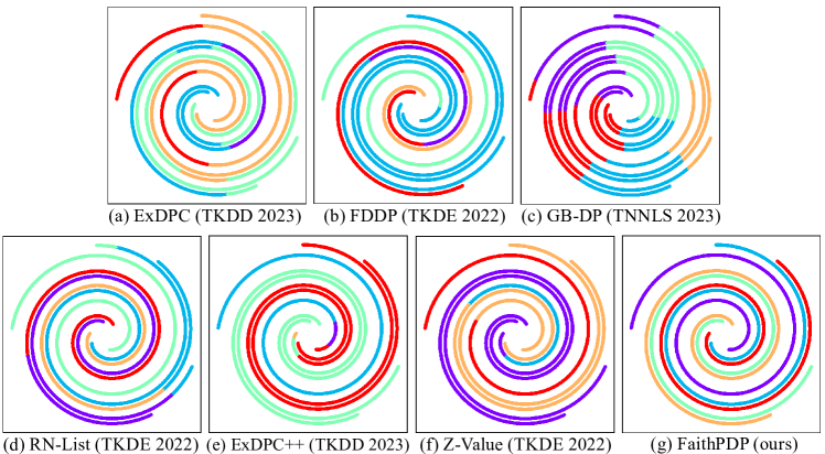
The two synthetic datasets are designed to demonstrate the accuracy and efficiency of FaithPDP. To better recognize the core advantage of FaithPDP, we visualize the clustering results of our method and six state-of-the-art counterparts in Fig. 3, from which one can find that FaithPDP is the only method that perfectly captures the subtle structure the spirals.
Performance on efficiency. We report the efficiency performance on three datasets that are representatives of two categories (considering number of samples and dimensionality) of dataset respectively. They are large amount with low dimension (DS1 and DS5) and Large amount with large dimension (DS7). For DS1 and DS5, the running time is visualized in Fig. 2, from which one can find FaithPDP achieves comparable time efficiency while generally being more accurate (refer to Table 2). For DS7, only GB-DP and FaithPDP can accomplish the clustering task on our experiment environment, the time assumptions are 37.95 seconds and 40.37 seconds, respectively.
Discussion. Table 2 shows that among eight datasets, FaithPDP wins the first place in accuracy for seven times and the second place once. The key insight is:
a) the exact family and list-index-based methods rely on cut-off kernel, hence emphasize on local neighbors while neglecting global distribution of entire dataset.
b) the methods combined with k-means first preprocess datapoints into spherical micro-clusters, hence lose the ability of DP to trace curve distribution (definitely exists in real world, although it is less common than spherical).
c) coding based methods (including Z-value and LSH) approximate map the original data into a new space, therefore they will be subjected to sacrifice of accuracy.
d) most existing methods compute the distances between data points in a pair-wise manner, thus causing relatively low efficiency.
FaithPDP addressed the issues mentioned above simultaneously, therefore achieved very promising accuracy and overall good time efficiency (slower only than GB-DP).
6 Conclusion
This paper presents a novel approach FaithPDP that takes advantages of both hardware (multi-core architecture of CPU) and modern programming language (Python or Matlab for efficient vector and matrix computation) to achieve clustering result identical to vanilla DP algorithm, while the computing complexity is reduced to pseudo-linear. FaithPDP addressed several issues raised by the existing counterparts simultaneously, a) preference to low-dimensional data by kd-tree based methods, b) degrading in accuracy by approximate approaches (k-means involved, LSH or Z-valued based), c) restricted to cut-off kernel in computing density by kd-tree and Index-list based methods. FaithPDP computing distance matrices in a matrix-computation manner other than pair-wise manner and utilize a inverse distance-density condition to find leading points. These two techniques enabled fast computation of density (compatible with both cut-off kernel and Gaussian kernel) and avoid memory requirement for storing the entire distance matrix, respectively. Extensive experiments show that FaithPDP has superior accuracy and comparable temporal and spacial efficiency against state-of-the-art methods.
Acknowledgement
This work has been supported by the National Natural Science Foundation of China under grants 62366008 and 61966005.
References
- [1] Dengyong Zhou and Christopher JC Burges. Spectral clustering and transductive learning with multiple views. In Proceedings of the 24th international conference on Machine learning, pages 1159–1166, 2007.
- [2] Yanwei Fu, Timothy M Hospedales, Tao Xiang, and Shaogang Gong. Transductive multi-view zero-shot learning. IEEE transactions on pattern analysis and machine intelligence, 37(11):2332–2345, 2015.
- [3] Yunfan Li, Peng Hu, Zitao Liu, Dezhong Peng, Joey Tianyi Zhou, and Xi Peng. Contrastive clustering. In Proceedings of the AAAI conference on artificial intelligence, volume 35, pages 8547–8555, 2021.
- [4] Vivek Sharma, Makarand Tapaswi, M Saquib Sarfraz, and Rainer Stiefelhagen. Clustering based contrastive learning for improving face representations. In 2020 15th IEEE International Conference on Automatic Face and Gesture Recognition (FG 2020), pages 109–116. IEEE, 2020.
- [5] Wanxia Deng, Qing Liao, Lingjun Zhao, Deke Guo, Gangyao Kuang, Dewen Hu, and Li Liu. Joint clustering and discriminative feature alignment for unsupervised domain adaptation. IEEE Transactions on Image Processing, 30:7842–7855, 2021.
- [6] Jian Liang, Ran He, Zhenan Sun, and Tieniu Tan. Aggregating randomized clustering-promoting invariant projections for domain adaptation. IEEE transactions on pattern analysis and machine intelligence, 41(5):1027–1042, 2019.
- [7] Guy Barrett Coleman and Harry C Andrews. Image segmentation by clustering. Proceedings of the IEEE, 67(5):773–785, 1979.
- [8] Guo Dong and Ming Xie. Color clustering and learning for image segmentation based on neural networks. IEEE transactions on neural networks, 16(4):925–936, 2005.
- [9] Yiming Tang, Fuji Ren, and Witold Pedrycz. Fuzzy c-means clustering through ssim and patch for image segmentation. Applied Soft Computing, 87:105928, 2020.
- [10] Chang-Dong Wang, Jian-Huang Lai, and S Yu Philip. Neiwalk: Community discovery in dynamic content-based networks. IEEE transactions on knowledge and data engineering, 26(7):1734–1748, 2014.
- [11] Yunyun Niu, Detian Kong, Ligang Liu, Rong Wen, and Jianhua Xiao. Overlapping community detection with adaptive density peaks clustering and iterative partition strategy. Expert Systems with Applications, 213:119213, 2023.
- [12] Aleksandr Farseev, Ivan Samborskii, Andrey Filchenkov, and Tat-Seng Chua. Cross-domain recommendation via clustering on multi-layer graphs. In Proceedings of the 40th international ACM SIGIR conference on research and development in information retrieval, pages 195–204, 2017.
- [13] Zhihua Cui, Xianghua Xu, XUE Fei, Xingjuan Cai, Yang Cao, Wensheng Zhang, and Jinjun Chen. Personalized recommendation system based on collaborative filtering for iot scenarios. IEEE Transactions on Services Computing, 13(4):685–695, 2020.
- [14] Alex Rodriguez and Alessandro Laio. Clustering by fast search and find of density peaks. science, 344(6191):1492–1496, 2014.
- [15] Daichi Amagata and Takahiro Hara. Efficient density-peaks clustering algorithms on static and dynamic data in euclidean space. ACM Transactions on Knowledge Discovery from Data, 18(1):1–27, 2023.
- [16] Jing Lu, Yuhai Zhao, Kian-Lee Tan, and Zhengkui Wang. Distributed density peaks clustering revisited. IEEE Transactions on Knowledge and Data Engineering, 34(8):3714–3726, 2022.
- [17] Yanfeng Zhang, Shimin Chen, and Ge Yu. Efficient distributed density peaks for clustering large data sets in mapreduce. IEEE Transactions on Knowledge and Data Engineering, 28(12):3218–3230, 2016.
- [18] Daichi Amagata and Takahiro Hara. Fast density-peaks clustering: multicore-based parallelization approach. In Proceedings of the 2021 International Conference on Management of Data, pages 49–61, 2021.
- [19] Dongdong Cheng, Ya Li, Shuyin Xia, Guoyin Wang, Jinlong Huang, and Sulan Zhang. A fast granular-ball-based density peaks clustering algorithm for large-scale data. IEEE Transactions on Neural Networks and Learning Systems, 2023.
- [20] Frank Nielsen. Introduction to mpi: the message passing interface. In Introduction to HPC with MPI for Data Science, pages 21–62. Springer, Switzerland, 2016.
- [21] Alina Beygelzimer, Sham Kakade, and John Langford. Cover trees for nearest neighbor. In Proceedings of the 23rd international conference on Machine learning, pages 97–104, 2006.
- [22] Liang Bai, Xueqi Cheng, Jiye Liang, Huawei Shen, and Yike Guo. Fast density clustering strategies based on the k-means algorithm. Pattern Recognition, 71:375–386, 2017.
- [23] Ji Xu, Guoyin Wang, and Weihui Deng. Denpehc: Density peak based efficient hierarchical clustering. Information Sciences, 373:200–218, 2016.
- [24] Ji Xu, Tianrui Li, Yongming Wu, and Guoyin Wang. Lapoleaf: Label propagation in an optimal leading forest. Inf. Sci., 575:133–154, 2021.
- [25] Message Passing Interface Forum. MPI: A Message-Passing Interface Standard Version 4.1, November 2023.
- [26] Lisandro Dalcín, Rodrigo Paz, and Mario Storti. Mpi for python. Journal of Parallel and Distributed Computing, 65(9):1108–1115, 2005.
- [27] Lisandro Dalcin and Yao-Lung L Fang. mpi4py: Status update after 12 years of development. Computing in Science & Engineering, 23(4):47–54, 2021.
- [28] Zafaryab Rasool, Rui Zhou, Lu Chen, Chengfei Liu, and Jiajie Xu. Index-based solutions for efficient density peak clustering. IEEE Transactions on Knowledge and Data Engineering, 34(5):2212–2226, 2022.
- [29] Alexander Strehl and Joydeep Ghosh. Cluster ensembles—a knowledge reuse framework for combining multiple partitions. Journal of machine learning research, 3(Dec):583–617, 2002.
- [30] Lawrence Hubert and Phipps Arabie. Comparing partitions. Journal of classification, 2:193–218, 1985.
- [31] Thomas Plötz, Nils Y Hammerla, and Patrick L Olivier. Feature learning for activity recognition in ubiquitous computing. In Twenty-second international joint conference on artificial intelligence, pages 1729–1734, 2011.