Stability of Data-Dependent Ridge-Regularization
for Inverse Problems

Abstract

Theoretical guarantees for the robust solution of inverse problems have important implications for applications. To achieve both guarantees and high reconstruction quality, we propose to learn a pixel-based ridge regularizer with a data-dependent and spatially-varying regularization strength. For this architecture, we establish the existence of solutions to the associated variational problem and the stability of its solution operator. Further, we prove that the reconstruction forms a maximum-a-posteriori approach. Simulations for biomedical imaging and material sciences demonstrate that the approach yields high-quality reconstructions even if only a small instance-specific training set is available.

Keywords: biomedical imaging, data-dependent regularization, data-driven priors, set-valued maps, spatial adaptivity, superresolution

1 Introduction

Inverse problems are ubiquitous in biomedical imaging [38], with examples such as magnetic resonance imaging and computed tomography. There, we aim to reconstruct an unknown image ${\mathbf{x}}\in\mathbb{R}^{n}$ from noisy measurements ${\mathbf{y}}=\mathrm{add_{n}}({\mathbf{H}}{\mathbf{x}})\in\mathbb{R}^{m}$, where ${\mathbf{H}}\in\mathbb{R}^{m,n}$ encodes the data-acquisition process, and the (possibly nonlinear) noise model $\mathrm{add_{n}}\colon\mathbb{R}^{m}\to\mathbb{R}^{m}$ accounts for imperfections in this description. One of the most common reconstruction methods is to solve a variational problem of the form

$$\hat{{\mathbf{x}}}=\operatorname*{arg\,min}_{{\mathbf{x}}\in\mathbb{R}^{n}}\bigl{(}\mathcal{D}({\mathbf{H}}{\mathbf{x}},{\mathbf{y}})+\lambda\mathcal{R}({\mathbf{x}})\bigr{)},$$ (1)

with a data-fidelity term $\mathcal{D}\colon\mathbb{R}^{m}\times\mathbb{R}^{m}\to\mathbb{R}_{\geq 0}$ and a regularizer $\mathcal{R}\colon\mathbb{R}^{n}\to\mathbb{R}_{\geq 0}$. In (1), the data term ensures the (approximate) consistency of the reconstruction $\hat{{\mathbf{x}}}$ with the observed data ${\mathbf{y}}$, while the regularizer $\mathcal{R}$, whose strength is controlled by $\lambda\in\mathbb{R}_{>0}$, promotes favorable properties of $\hat{{\mathbf{x}}}$.

For many acquisition operators ${\mathbf{H}}$ and noise models $\mathrm{add_{n}}$, well-suited loss functions $\mathcal{D}$ exist [48, 52]. While $\mathcal{D}$ is instance-specific, $\mathcal{R}$ is preferably agnostic to ${\mathbf{H}}$ and $\mathrm{add_{n}}$. In particular, $\mathcal{R}$ should depend exclusively on the properties of the underlying images. Attempts in this direction go back to the Tikhonov regularization [54], where images are modeled as smooth signals. Over the years, better regularizers such as total variation [51], compressed sensing [13] and the field-of-experts [50] have been developed. More recently, learned regularizers such as adversarial ones [36, 39, 53], patch priors [1, 46], plug-and-play priors [20, 24, 23], network Tikhonov [34] or total deep variation [29, 30] led to huge improvements in reconstruction quality. To maintain interpretability, the works [16, 17] instead learn simple regularizers of the form

$$\mathcal{R}\colon{\mathbf{x}}\mapsto\sum_{c=1}^{N_{\mathrm{C}}}\bigl{\langle}\bm{1}_{n},\bm{\psi}_{c}({\mathbf{W}}_{c}{\mathbf{x}})\bigr{\rangle},$$ (2)

with convolution matrices ${\mathbf{W}}_{c}\in\mathbb{R}^{n,n}$ and potentials $\bm{\psi}_{c}({\mathbf{x}})=(\psi_{c}(x_{k}))_{k=1}^{n}$ with $\psi_{c}\in\mathcal{C}_{\geq 0}^{1,1}(\mathbb{R})$, where $\mathcal{C}_{\geq 0}^{1,1}(\mathbb{R})$ is the space of nonnegative differentiable functions with Lipschitz-continuous derivatives. As shorthand, we introduce the notation ${\mathbf{W}}=({\mathbf{W}}_{c})_{c=1}^{N_{C}}$ and $\bm{\psi}=(\bm{\psi}_{c})_{c=1}^{N_{C}}$. While [16] only deployed convex $\psi_{c}$ in (2), leading to a convex regularizer, more general $1$-weakly convex profiles ($\psi_{c}^{\prime\prime}>-1$) significantly boost the performance [17]. If $\lambda\leq 1$, the objective (1) remains convex for image denoising (${\mathbf{H}}={\mathbf{I}}$) even in the weakly convex setting. Hence, it is easy to minimize. Due to its clear interpretability as a filter-based model, we choose (2) as the starting point for our investigation.

So far, the regularization strength in (2) is the same for each pixel and every channel. However, starting with total-variation regularization [12, 21, 57], it has been observed in several works (see for example [31, 32, 62] in the data-driven setting) that the use of a spatially-adaptive regularization strength (as opposed to $\bm{1}_{n}$) can significantly boost the performance of the reconstruction model (1). Following this idea, a data-dependent generalization of (2) was recently proposed in [41] as

$$\mathcal{R}_{{\mathbf{y}}}\colon{\mathbf{x}}\mapsto\sum_{c=1}^{N_{\mathrm{C}}}\bigl{\langle}\bm{\Lambda}_{c}({\mathbf{y}}),\bm{\psi}_{c}({\mathbf{W}}_{c}{\mathbf{x}})\bigr{\rangle},$$ (3)

where the mask $\bm{\Lambda}=({\mathbf{\Lambda}}_{c})_{c=1}^{N_{C}}$ with $\bm{\Lambda}_{c}\colon\mathbb{R}^{n}\to[\epsilon,1]^{n}$ and $\epsilon>0$ makes (3) data-dependent without increasing the weak-convexity modulus compared to $\mathcal{R}$. So far, only weakly convex $\psi_{c}$ have been studied, likely because they lead to a better baseline model. For (3), the spatial adaptivity can be motivated as follows. First, the noise might be non-uniform across the data, such that a local adaption of the regularization strength becomes necessary. Further, the pixel-wise cost $\mathcal{R}_{{\mathbf{y}}}$ often over-penalizes structure, which leads to smoothing. As structure might only respond to certain ${\mathbf{W}}_{c}$, it is reasonable to use different masks across the channels. For a more detailed overview, we refer to [45].

Nowadays, classic signal-processing approaches often serve as a basic benchmark. For such regularizers, the reconstruction model (1) is stable and converges for vanishing noise [52, 10]. Guarantees of this type play a crucial role in applications such as medical imaging, where diagnostic decisions are based on the provided reconstructions. While the classic approaches are well-understood, many questions remain open for learned ones. In particular, learned approaches might hallucinate or remove meaningful structures [28]. If the network-based $\mathcal{R}$ does not depend on the data, some (weaker) theoretical guarantees exist [34, 40, 42, 53]. For data-dependent regularizers $\mathcal{R}_{{\mathbf{y}}}$, like the one in (3), such an analysis is to the best of our knowledge unavailable. While some ideas from previous work are transferable, other aspects need a completely new treatment.

Contribution and Outline

In Section 3, we prove existence, stability and convergence for vanishing noise of critical points for the reconstruction model (1) with $\mathcal{R}_{{\mathbf{y}}}$ of the form (3). To deal with the non-uniqueness of critical points, we use the theory of implicit multifunctions [14, 26], for which a generic stability analysis exists [15, 7]. Due to the specific structure of $\mathcal{R}_{{\mathbf{y}}}$, we can derive yet stronger results by using tools from variational analysis directly. Our Lipschitz-like results are also stronger compared to the ones in previous works on learned regularization. The relevant stability concepts for set-valued maps and the necessary tools from variational analysis are summarized in Section 2. Note that all stability concepts generalize the Lipschitz continuity of single-valued functions.

Let us briefly discuss the results from Section 3 ordered according to their strength. Naturally, the strongest one (see Section 3.1) is obtained if the Hessian of the objective in (1) is locally invertible around critical points. Then, the critical points are isolated and each one depends Lipschitz continuously on the data ${\mathbf{y}}$. Unfortunately, the local invertibility is hard to guarantee in practice. Therefore, we also investigate two other settings. In Section 3.2, we establish the outer Lipschitz continuity (one of the set-valued generalizations) for the case $\bm{\Lambda}_{c}({\mathbf{y}})=\bm{1}_{n}$ and piecewise quadratic profiles. Then, the data-to-reconstruction map is polyhedral, which ensures many favorable properties that general set-valued maps do not have. As a second setting, we analyze (data-dependent) convex regularizers $\mathcal{R}_{{\mathbf{y}}}$ in Section 3.3. First, we sharpen the results from Section 3.2 to (set-valued) Lipschitz continuity using the convexity. Further, for a data-dependent mask $\bm{\Lambda}({\mathbf{y}})$, we derive a weaker localized version of the Lipschitz continuity (namely the Aubin property). To complement the stability analysis, we consider the vanishing noise setting in Section 3.4. After this well-posedness discussion, a Bayesian interpretation of the model (1) is established in Section 3.5. Here, we show that the regularizer (3) induces a probability density and that (1) is a maximum-a-posteriori approach.

Our theoretical results for convex $\psi_{c}$ in (3) are stronger than with weakly convex ones. Hence, one might wonder how this restriction affects the practical performance. One possible explanation for the increase in performance with weakly convex $\psi_{c}$ is that these reduce the over-penalization of structure. In view of this, a data-dependent mask $\bm{\Lambda}$ is an alternative approach to deal with this issue. To understand the interactions, we learn $\bm{\Lambda}$ for both the convex and the weakly convex regularizer, and compare the resulting denoising performance in Section 5.1. Interestingly, the obtained results are very similar and far superior to the weakly convex regularizer with $\bm{\Lambda}_{c}({\mathbf{y}})=\bm{1}_{n}$.

Encouraged by these findings, we extend the experimental validation made in [41] for magnetic resonance imaging, which is revisited in Section 5.2, to two new tasks, namely computed tomography in Section 5.3 and superresolution of material microstructures in Section 5.4. For these tasks, we usually lack a large training database because of privacy preservation in medical imaging or destructive/costly processes in material sciences. Hence, we learn the data-dependent $\mathcal{R}_{{\mathbf{y}}}$ from a generic image database such as BSD500, intending to learn a universal regularizer. Then, we only fine-tune the regularization strength $\bm{\Lambda}$ in the learned $\mathcal{R}_{{\mathbf{y}}}$ for the task at hand if data is available. In our simulations, this leads to high-quality reconstructions with only a small instance specific training set.

2 A Brief on Set-Valued Maps

We start with some general notation. The closed unit ball in $\mathbb{R}^{n}$ is denoted by $\mathbb{B}$. The collection of all subsets $N$ of $\mathbb{N}$ such that $\mathbb{N}\backslash N$ is finite is denoted by $\mathscr{N}$, whereas the collection of all infinite $N\subset\mathbb{N}$ is denoted by $\mathscr{N}^{\sharp}$. With this, we can conveniently handle subsequences of a given sequence. For instance, if we have $\{{\mathbf{x}}_{k}\}_{k\in\mathbb{N}}\subset\mathbb{R}^{n}$, then $\{{\mathbf{x}}_{k}\}_{k\in N}$ for either $N\in\mathscr{N}$ or $N\in\mathscr{N}^{\sharp}$ designates a subsequence. Limits as $k\rightarrow\infty$ with $k\in N$ are either indicated by $\lim_{k\in N}$ or with arrows by $\xrightarrow{N}$. The function $\mathbf{diag}\colon\mathbb{R}^{n}\to\mathbb{R}^{n,n}$ returns a diagonal matrix whose diagonal entries are the input vector.

Set-Valued Maps

Set-valued maps $S\colon\mathbb{R}^{m}\rightrightarrows\mathbb{R}^{n}$ appear as solution operators to (1). For an in-depth introduction, we refer to [14, Cha. 3]. The set $\mathrm{dom}(S)=\{{\mathbf{y}}\in\mathbb{R}^{m}:S({\mathbf{y}})\neq\emptyset\}$ is the domain of $S$, and the graph of $S$ is the set $\operatorname{Graph}(S)=\{({\mathbf{y}},{\mathbf{x}})\in\mathbb{R}^{m}\times\mathbb{R}^{n}:{\mathbf{x}}\in S({\mathbf{y}})\}$. The inverse $S^{-1}\colon\mathbb{R}^{n}\rightrightarrows\mathbb{R}^{m}$ of $S$ is defined via $\operatorname{Graph}(S^{-1})=\{({\mathbf{x}},{\mathbf{y}})\in\mathbb{R}^{n}\times\mathbb{R}^{m}:({\mathbf{y}},{\mathbf{x}})\in\operatorname{Graph}(S)\}$. Recall that

$$\limsup_{{\mathbf{y}}\rightarrow\bar{{\mathbf{y}}}}S({\mathbf{y}})=\left\{{\mathbf{x}}:\exists{\mathbf{y}}_{k}\rightarrow\bar{{\mathbf{y}}},\exists{\mathbf{x}}_{k}\rightarrow{\mathbf{x}}\text{ with }{\mathbf{x}}_{k}\in S\left({\mathbf{y}}_{k}\right)\right\}$$ (4)

and

$$\liminf_{{\mathbf{y}}\rightarrow\bar{{\mathbf{y}}}}S({\mathbf{y}})=\bigl{\{}{\mathbf{x}}:\forall{\mathbf{y}}_{k}\rightarrow\bar{{\mathbf{y}}},\exists N\in\mathscr{N},{\mathbf{x}}_{k}\xrightarrow{N}{\mathbf{x}}\text{ with }{\mathbf{x}}_{k}\in S\left({\mathbf{y}}_{k}\right)\bigr{\}}.$$ (5)

Now, we discuss several notions of continuity. A map $S$ is outer semicontinuous (osc) relative to $D\subset\mathrm{dom}(S)$ at $\bar{{\mathbf{y}}}\in\mathbb{R}^{m}$ if $\limsup_{{\mathbf{y}}\rightarrow\bar{{\mathbf{y}}}}S({\mathbf{y}})\subset S(\bar{{\mathbf{y}}})$, where the sequences are taken in $D$. This is equivalent to $\operatorname{Graph}(S)$ being closed in $D\times\mathbb{R}^{n}$. Further, $S$ is inner semicontinuous (isc) relative to $D$ at $\bar{{\mathbf{y}}}$ if $\liminf_{{\mathbf{y}}\rightarrow\bar{{\mathbf{y}}}}S({\mathbf{y}})\supset S(\bar{{\mathbf{y}}})$. This is equivalent to $S^{-1}(O)$ being open in D for every open $O\subset\mathbb{R}^{n}$. Finally, $S$ is continuous relative to $D$ at $\bar{{\mathbf{y}}}$ iff it is both osc and isc relative to $D$. For single-valued $S$, this coincides with the usual notion of continuity. Conversely, any closed-convex-valued and isc $S$ admits a continuous single-valued selection $\tilde{S}\colon\mathrm{dom}(S)\to\mathbb{R}^{n}$, see [14, Thm. 5J.5].

The map $S$ is Lipschitz continuous relative to $D\subset\mathrm{dom}(S)$ if $S$ is closed-valued, and there exists a Lipschitz constant $\kappa>0$ such that

$$S({\mathbf{y}}^{\prime})\subset S({\mathbf{y}})+\kappa\|{\mathbf{y}}^{\prime}-{\mathbf{y}}\|\mathbb{B}\quad\text{ for all }{\mathbf{y}}^{\prime},{\mathbf{y}}\in D.$$ (6)

Lipschitz continuity is closely related to strict continuity of $S$ at $\bar{{\mathbf{y}}}$, which means that for each $\rho>0$, there exist $\kappa>0$ and a neighbourhood $V$ of $\bar{{\mathbf{y}}}$ such that

$$S({\mathbf{y}})\cap\rho\mathbb{B}\subset S({\mathbf{y}}^{\prime})+\kappa\|{\mathbf{y}}-{\mathbf{y}}^{\prime}\|\mathbb{B}\quad\text{ for all }{\mathbf{y}},{\mathbf{y}}^{\prime}\in V.$$ (7)

The difference to (6) is the intersection with $\rho\mathbb{B}$, which resolves issues that can arise if $S$ takes unbounded sets as value. As a local counterpart to (7), we say that $S$ has the Aubin (or Lipschitz-like) property at $\bar{{\mathbf{y}}}$ for $\bar{{\mathbf{x}}}\in S(\bar{{\mathbf{y}}})$ if $\operatorname{Graph}(S)$ is locally closed at $(\bar{{\mathbf{y}}},\bar{{\mathbf{x}}})$, and there is $\kappa>0$ along with neighborhoods $V$ of $\bar{{\mathbf{y}}}$ and $U$ of $\bar{{\mathbf{x}}}$ such that

$$S({\mathbf{y}}^{\prime})\cap U\subset S({\mathbf{y}})+\kappa\|{\mathbf{y}}^{\prime}-{\mathbf{y}}\|\mathbb{B}\quad\text{ for all }{\mathbf{y}}^{\prime},{\mathbf{y}}\in V.$$ (8)

For single valued maps, all the concepts (6)-(8) coincide with the usual Lipschitz continuity.

Next, we introduce weaker continuity notations, where the reference point ${\mathbf{y}}$ in the right hand sides of (6) and (8) is fixed. The map $S$ is outer Lipschitz continuous at $\bar{{\mathbf{y}}}\in D$ relative to $D\subset\mathrm{dom}(S)$ if $S(\bar{{\mathbf{y}}})$ is closed, and there is $\kappa>0$ along with a neighborhood $V$ of $\bar{{\mathbf{y}}}$ such that

$$S({\mathbf{y}})\subset S(\bar{{\mathbf{y}}})+\kappa\|{\mathbf{y}}-\bar{{\mathbf{y}}}\|\mathbb{B}\quad\text{ for all }{\mathbf{y}}\in V\cap D.$$ (9)

If $S$ is outer Lipschitz continuous at every ${\mathbf{y}}\in D$ with the same $\kappa$, then $S$ is outer Lipschitz continuous relative to $D$. A yet weaker notion originates from (8). The map $S$ is calm at $(\bar{{\mathbf{y}}},\bar{{\mathbf{x}}})\in\operatorname{Graph}(S)$ if there is $\kappa>0$ along with neighborhoods $V$ of $\bar{{\mathbf{y}}}$ and $U$ of $\bar{{\mathbf{x}}}$ such that

$$S({\mathbf{y}})\cap U\subset S(\bar{{\mathbf{y}}})+\kappa\|{\mathbf{y}}-\bar{{\mathbf{y}}}\|\mathbb{B}\quad\text{ for all }{\mathbf{y}}\in V.$$ (10)

Compared with (9), the inclusion only holds locally, similar to the relation between the Lipschitz continuity and the Aubin property.

An important class of set-valued maps $S$ are polyhedral ones, for which $\operatorname{Graph}(S)$ is a finite union of polyhedra. Recall that a polyhedron in $\mathbb{R}^{m+n}$ is of the form $\{{\mathbf{x}}\in\mathbb{R}^{m+n}:{\mathbf{A}}{\mathbf{x}}\leq{\mathbf{b}}\}$ with ${\mathbf{A}}\in\mathbb{R}^{p,m+n}$ and ${\mathbf{b}}\in\mathbb{R}^{p}$. Polyhedral maps are strictly continuous outside of a lower-dimensional set $D$ ($\dim(D)<m$) and the Lipschitz modulus $\kappa$ can be chosen independent of $\bar{{\mathbf{y}}}$ [9, Prop. 35]. Moreover, they are outer Lipschitz continuous with a uniform modulus [14, Thm. 3D.1].

Hoffman bound

The Hoffman bound [22] in the formulation of [43, Props. 5 and 6] states that for ${\mathbf{E}}\in\mathbb{R}^{n,n}$, ${\mathbf{F}}\in\mathbb{R}^{l,n}$, ${\mathbf{b}}\in\mathbb{R}^{n}$ and ${\mathbf{q}}\in\mathbb{R}^{l}$ with $\{{\mathbf{x}}\in\mathbb{R}^{n}:{\mathbf{E}}{\mathbf{x}}={\mathbf{b}},{\mathbf{F}}{\mathbf{x}}\leq{\mathbf{q}}\}\neq\emptyset$ and any ${\mathbf{x}}^{\prime}\in\mathbb{R}^{n}$ it holds that

$$\min_{{\mathbf{E}}{\mathbf{x}}={\mathbf{b}},{\mathbf{F}}{\mathbf{x}}\leq{\mathbf{q}}}\|{\mathbf{x}}-{\mathbf{x}}^{\prime}\|\leq K({\mathbf{E}},{\mathbf{F}})\biggl{\|}\begin{pmatrix}{\mathbf{E}}{\mathbf{x}}^{\prime}-{\mathbf{b}}\\ ({\mathbf{F}}{\mathbf{x}}^{\prime}-{\mathbf{q}})_{+}\end{pmatrix}\biggr{\|},$$ (11)

where

$$K({\mathbf{E}},{\mathbf{F}}) =\max_{J\in U({\mathbf{E}},{\mathbf{F}})}\biggl{(}\min\Bigl{\{}\bigl{\|}{\mathbf{E}}^{T}{\mathbf{u}}+({\mathbf{F}}_{J})^{T}{\mathbf{v}}\bigr{\|}:{\mathbf{u}}\in\mathrm{ran}({\mathbf{E}}),\,{\mathbf{v}}\geq 0,\,\|({\mathbf{u}},{\mathbf{v}})\|=1\Bigr{\}}\biggr{)}^{-1}<\infty.$$ (12)

In (12), $U({\mathbf{E}},{\mathbf{F}})$ consists of the subsets of $\{1,\ldots,l\}$ (denoted by $[l]$) for which the corresponding rows of ${\mathbf{F}}$ are linearly independent and $\mathrm{ran}({\mathbf{E}}^{T})\cap\mathrm{ran}({\mathbf{F}}_{J}^{T})=\{{\mathbf{0}}\}$. Indeed, the notation of [43] simplifies for our specific setting $R=\mathbb{R}^{n}$ as follows

$$S({\mathbf{F}},{\mathbf{E}}|\mathbb{R}^{n})= \bigl{\{}(J,\mathbb{R}^{n}):J\subset[l],\{({\mathbf{F}}{\mathbf{x}}+{\mathbf{s}},{\mathbf{E}}{\mathbf{x}}):{\mathbf{x}}\in\mathbb{R}^{n},{\mathbf{s}}\in\mathbb{R}^{l},s_{J}\geq 0\}\text{ is a linear subspace}\bigr{\}}$$

$$= \bigl{\{}(J,\mathbb{R}^{n}):J\subset[l],\{({\mathbf{F}}_{J}{\mathbf{x}}+{\mathbf{s}},{\mathbf{E}}{\mathbf{x}}):{\mathbf{x}}\in\mathbb{R}^{n},{\mathbf{s}}\in\mathbb{R}_{\geq 0}^{|J|}\}=\mathbb{R}^{|J|}\times\mathrm{ran}({\mathbf{E}})\bigr{\}}$$

$$= \bigl{\{}(J,\mathbb{R}^{n}):J\subset[l],\{({\mathbf{F}}_{J}{\mathbf{x}},{\mathbf{E}}{\mathbf{x}}):{\mathbf{x}}\in\mathbb{R}^{n}\}=\mathbb{R}^{|J|}\times\mathrm{ran}({\mathbf{E}})\bigr{\}}$$

$$= \{(J,\mathbb{R}^{n}):J\in U({\mathbf{E}},{\mathbf{F}})\}.$$ (13)

Since the estimate (11) bounds the distance to the polyhedra $\{{\mathbf{x}}\in\mathbb{R}^{n}:{\mathbf{E}}{\mathbf{x}}={\mathbf{b}},{\mathbf{F}}{\mathbf{x}}\leq{\mathbf{q}}\}$, it is useful for estimating the Lipschitz constant of polyhedral maps.

Implicit Set-Valued Maps

Given a Lipschitz continuous function $f\colon\mathbb{R}^{m+n}\to\mathbb{R}^{n}$, we can implicitly define a set-valued map $S\colon\mathbb{R}^{m}\rightrightarrows\mathbb{R}^{n}$ via

$$S({\mathbf{y}})=\bigl{\{}{\mathbf{x}}\in\mathbb{R}^{n}:f({\mathbf{y}},{\mathbf{x}})=0\bigr{\}}.$$ (14)

In this paper, $f$ is induced by the optimization problem (1). Strong regularity statements for $S$ can be made if $f$ is sufficiently smooth. The classical implicit function theorem with regular $f\in C^{1}(\mathbb{R}^{m+n},\mathbb{R}^{n})$ guarantees that $S$ exists and admits single-valued localizations. Moreover, each localization is differentiable and there is a formula for its derivative. If $f$ is merely Lipschitz continuous, Clarke’s implicit function theorem [6] guarantees existence of localizations together with their Lipschitz continuity. The theorem requires the partial invertibility of the Clarke Jacobian

$$J_{f}^{c}({\mathbf{y}},{\mathbf{x}})=\mathrm{conv}\bigl{\{}{\mathbf{V}}\in\mathbb{R}^{m+n,n}:\exists({\mathbf{y}}_{k},{\mathbf{x}}_{k})\in R\text{ with }({\mathbf{y}}_{k},{\mathbf{x}}_{k})\to({\mathbf{y}},{\mathbf{x}})\text{ s.t. }J_{f}({\mathbf{y}}_{k},{\mathbf{x}}_{k})\to{\mathbf{V}}\bigr{\}},$$ (15)

where $R\subset\mathbb{R}^{m+n}\times\mathbb{R}^{n}$ is the set of full measure on which $f$ is differentiable (Rademacher theorem). Unfortunately, there is no formula for the Clarke Jacobian $J_{S}^{c}$ of $S$. Recently, an improved implicit function theorem based on conservative Jacobians was established in [4]. We say that $J_{f}\colon\mathbb{R}^{m+n}\rightrightarrows\mathbb{R}^{n,m+n}$ is a conservative Jacobian for $f$ if $\operatorname{Graph}(J_{f})$ is closed, locally bounded, and nonempty with

$$\frac{\mathrm{d}}{\mathrm{d}t}f\circ\gamma(t)={\mathbf{V}}\gamma^{\prime}(t)\quad\text{ for all }{\mathbf{V}}\in J_{f}(\gamma(t))\text{ and a.e.\ }t,$$ (16)

where $\gamma$ is an absolutely continuous curve in $\mathbb{R}^{m+n}$. The convex hull of any $J_{f}({\mathbf{y}},{\mathbf{x}})$ is a superset of $J_{f}^{c}({\mathbf{y}},{\mathbf{x}})$ and coincides with the usual Jacobian on $R$. Compared to Clarke Jacobians, conservative Jacobians come with a proper calculus [3]. This makes their computation much easier, since we can decompose complicated functions into simpler components. Note that a $J_{f}$ is usually not unique.

Theorem 1 (Implicit function theorem [4]).

Let $f\colon\mathbb{R}^{m+n}\to\mathbb{R}^{n}$ with a conservative Jacobian $J_{f}$ and $(\bar{{\mathbf{y}}},\bar{{\mathbf{x}}})\in\mathbb{R}^{m+n}$ be such that $f(\bar{{\mathbf{y}}},\bar{{\mathbf{x}}})=0$. Assume that $J_{f}(\bar{{\mathbf{y}}},\bar{{\mathbf{x}}})$ is convex and that for each $\begin{pmatrix}{\mathbf{A}}&{\mathbf{B}}\end{pmatrix}\in J_{f}(\bar{{\mathbf{y}}},\bar{{\mathbf{x}}})$ the matrix ${\mathbf{B}}$ is invertible. Then, there exists an open neighborhood $U\times V\subset\mathbb{R}^{m+n}$ of $(\bar{{\mathbf{y}}},\bar{{\mathbf{x}}})$ and $S\colon U\to V$ with a conservative Jacobian $J_{S}$ such that $f(\bar{{\mathbf{y}}},S(\bar{{\mathbf{y}}}))=0$. If for each ${\mathbf{y}}\in U$ and $\begin{pmatrix}{\mathbf{A}}&{\mathbf{B}}\end{pmatrix}\in J_{f}({\mathbf{y}},S({\mathbf{y}}))$ the matrix ${\mathbf{B}}$ is invertible, then a possible $J_{S}$ is given by

$$J_{S}\colon{\mathbf{y}}\rightrightarrows\bigl{\{}-{\mathbf{B}}^{-1}{\mathbf{A}}:\begin{pmatrix}{\mathbf{A}}&{\mathbf{B}}\end{pmatrix}\in J_{f}({\mathbf{y}},S({\mathbf{y}}))\bigr{\}}.$$ (17)

In principle, the minimal $J_{f}$ for Theorem 1 is $J^{c}_{f}$ [3, Cor. 1], which might be impossible to compute. With the (possibly larger) conservative Jacobians, we gain flexibility at the cost of having to check the invertibility of more elements. If $f$ does not have a partially invertible $J_{f}$, we can instead rely on the more general implicit function theorem discussed in [14, 26]. The following theorem guarantees the Aubin property instead of Lipschitz continuity like before.

Theorem 2 (Implicit function theorem [26, Thm. 2.84]).

Let $f\colon\mathbb{R}^{m+n}\to\mathbb{R}^{n}$ and $f(\bar{{\mathbf{y}}},\bar{{\mathbf{x}}})=0$. Suppose that

• for all ${\mathbf{y}}$ in a neighborhood of $\bar{{\mathbf{y}}}$, the partial inverse $f^{-1}({\mathbf{y}},\cdot)\colon\mathbb{R}^{n}\rightrightarrows\mathbb{R}^{n}$ is K-calm at $0$ for $\bar{{\mathbf{x}}}$;

• $f(\cdot,{\mathbf{x}})$ is $\alpha$-Lipschitz for all ${\mathbf{x}}$ in some neighborhood of $\bar{{\mathbf{x}}}$.

Then, $S$ has the Aubin property near $(\bar{{\mathbf{y}}},\bar{{\mathbf{x}}})$ and $\kappa\leq K\alpha$, see also (8).

Here, we replaced the metric subregularity of $f$ by the equivalent calmness of $f^{-1}$ for convenience of notation, see [14, Thm. 3H.3]. In theory, a necessary and sufficient condition for the Aubin property is given by the Mordukhovich criterion [49, Thm. 9.40]. However, the involved coderivatives of $S$ are difficult to compute, see [15] for a recent discussion, so that we prefer to rely on Theorem 2 instead. For polyhedral $f$, also $S$ is polyhedral, and we require neither of these tools.

3 Theoretical Properties of Ridge Regularizers

For the theoretical analysis, we restrict ourselves to data terms $\mathcal{D}_{P}\colon\mathbb{R}^{m}\times\mathbb{R}^{m}\to\mathbb{R}_{\geq 0}$ of the form

$$\mathcal{D}_{P}({\mathbf{H}}{\mathbf{x}},{\mathbf{y}})=\sum_{j=1}^{m}\phi_{j}\bigl{(}({\mathbf{H}}{\mathbf{x}})_{j},y_{j}\bigr{)}=\bigl{\langle}\bm{1}_{m},\bm{\phi}({\mathbf{H}}{\mathbf{x}},{\mathbf{y}})\bigr{\rangle},$$ (18)

where $\bm{\phi}({\mathbf{x}},{\mathbf{y}})=(\phi_{j}(x_{j},y_{j}))_{j=1}^{m}$ and the functions $\phi_{j}\in\mathcal{C}_{\geq 0}^{1,1}(\mathbb{R}^{2})$ are piecewise-polynomial with finitely many pieces. The probably most popular instance of this form is $\mathcal{D}_{P}({\mathbf{H}}{\mathbf{x}},{\mathbf{y}})=\frac{1}{2}\|{\mathbf{H}}{\mathbf{x}}-{\mathbf{y}}\|^{2}$. Together with the regularizer (3), where the profiles $\psi_{c}\in\mathcal{C}_{\geq 0}^{1,1}(\mathbb{R})$ are piecewise-polynomial, we arrive at

$$\operatorname*{arg\,min}_{{\mathbf{x}}\in\mathcal{X}}\Big{(}g_{{\mathbf{y}}}({\mathbf{x}})\coloneqq\mathcal{D}_{P}({\mathbf{H}}{\mathbf{x}},{\mathbf{y}})+\lambda\sum_{c=1}^{N_{\mathrm{C}}}\bigl{\langle}\bm{\Lambda}_{c}({\mathbf{y}}),\bm{\psi}_{c}({\mathbf{W}}_{c}{\mathbf{x}})\bigr{\rangle}\Big{)}.$$ (19)

Here, we assume that the masks $\bm{\Lambda}_{c}\colon\mathbb{R}^{m}\to[\epsilon,1]^{n}$ with $\epsilon>0$ are Lipschitz continuous. Due to the upper-bound by $1$, the $\bm{\Lambda}$ does not increase the weak-convexity modulus compared to $\mathcal{R}$. Since Theorem 8 requires coercivity of $\mathcal{R}_{{\mathbf{y}}}$, we provide a suffcient condition for it.

Lemma 1.

The function $g_{{\mathbf{y}}}$ in (19) is coercive if $\ker({\mathbf{W}})\cap\ker({\mathbf{H}})=\{0\}$ and all $\phi_{j}$ and $\psi_{c}$, $j=1,...,m$, $c=1,...,N_{c}$ are coercive.

Proof.

Let $\{{\mathbf{x}}_{k}\}_{k\in\mathbb{N}}$ with $\|{\mathbf{x}}_{k}\|\to\infty$. Then, either $\|{\mathbf{H}}{\mathbf{x}}_{k}\|\to\infty$ or there exists $c$ with $\|{\mathbf{W}}_{c}{\mathbf{x}}_{k}\|\to\infty$. Due to the coercivity of the $\phi_{j}$ and $\psi_{c}$, the claim readily follows. ∎

We have that (19) is nonempty if the profiles $\psi_{c}$ are piecewise-polynomial.

Theorem 3 (Existence).

Let $\psi_{c}\in\mathcal{C}_{\geq 0}^{1,1}(\mathbb{R})$, $c=1,\ldots,N_{C}$, be piecewise-polynomial with finitely many pieces, and $\mathcal{X}\subset\mathbb{R}^{n}$ be a polyhedron. Then, (19) is nonempty.

Proof.

Since the functions $\psi_{c}$ and $\phi_{j}(\cdot,y_{j})$ are piecewise polynomial, they partition $\mathbb{R}$ into finitely many closed intervals $(I_{l})_{l=1}^{L}$ on which they are polynomials. Hence, if we denote the $i$-th row of ${\mathbf{W}}_{c}$ and ${\mathbf{H}}$ with ${\mathbf{W}}_{c,i}$ and ${\mathbf{H}}_{i}$, respectively, then $\psi_{c}({\mathbf{W}}_{c,i}\cdot)$ and $\phi_{j}({\mathbf{H}}_{j}\cdot,y_{j})$ partition $\mathcal{X}$ into $L$ polyhedra $A_{c,i}^{l}=\{{\mathbf{x}}\in\mathcal{X}:{\mathbf{W}}_{c,i}{\mathbf{x}}\in I_{l}\}$ and $B_{j}^{l}=\{{\mathbf{x}}\in\mathcal{X}:{\mathbf{H}}_{j}{\mathbf{x}}\in I_{l}\}$, respectively. By intersecting over all possible combinations of $c$, $i$, and $j$, we get a finite decomposition of $\mathcal{X}$ into polyhedra on which $g_{{\mathbf{y}}}$ is a polynomial. The infimum of $g_{{\mathbf{y}}}$ is attained on (at least) one polyhedron, which we denote with $P$.

Now, we pick a minimizing sequence $\{{\mathbf{x}}_{k}\}_{k\in\mathbb{N}}\subset P$. Let ${\mathbf{M}}$ be the matrix which is the vertical concatenation of ${\mathbf{H}}_{j}$ and all ${\mathbf{W}}_{c,i}$ with $c$ and rows $i$ and $j$ such that $\{{\mathbf{W}}_{c,i}{\mathbf{x}}_{k}\}_{k\in\mathbb{N}}$ and $\{{\mathbf{H}}_{j}{\mathbf{x}}_{k}\}_{k\in\mathbb{N}}$ remain bounded. Since $\{{\mathbf{M}}{\mathbf{x}}_{k}\}_{k\in\mathbb{N}}$ is bounded by construction, we can extract a convergent subsequence indexed by $N\in\mathscr{N}^{\sharp}$ with limit ${\mathbf{u}}\in\mathrm{ran}({\mathbf{M}})$. The associated set

$$Q=\{{\mathbf{x}}\in\mathbb{R}^{n}\colon{\mathbf{M}}{\mathbf{x}}={\mathbf{u}}\}=\{{\mathbf{M}}^{\dagger}{\mathbf{u}}\}+\ker({\mathbf{M}})$$ (20)

is a polyhedron. It holds that

$$\mathrm{dist}({\mathbf{x}}_{k},Q)=\mathrm{dist}\bigl{(}{\mathbf{M}}^{\dagger}{\mathbf{M}}{\mathbf{x}}_{k}+\mathrm{P}_{\ker({\mathbf{M}})}({\mathbf{x}}_{k}),Q\bigr{)}\leq\|{\mathbf{M}}^{\dagger}{\mathbf{M}}{\mathbf{x}}_{k}-{\mathbf{M}}^{\dagger}{\mathbf{u}}\|\xrightarrow{N}0$$ (21)

and, thus, that $\mathrm{dist}(P,Q)=0$, which is only possible if $P\cap Q\neq\emptyset$ [59, Thm. 1].

The rows ${\mathbf{W}}_{c,i}$ and ${\mathbf{H}}_{j}$ that were not added to ${\mathbf{M}}$ satisfy $|{\mathbf{W}}_{c,i}{\mathbf{x}}_{k}|\to\infty$ and $|{\mathbf{H}}_{j}{\mathbf{x}}_{k}|\to\infty$ as $k\to\infty$. Hence, they are contained in unbounded intervals $I_{l_{c,i}}$ and $I_{l_{j}}$, respectively. Since $\psi_{c}$ and $\phi_{j}(\cdot,y_{j})$ are nonnegative polynomials on them, $\psi_{c}({\mathbf{W}}_{c,i}\cdot)$ and $\phi_{j}({\mathbf{H}}_{j}\cdot,y_{j})$ are constant on $P$. Hence, $\lim_{k\to\infty}\psi_{c}({\mathbf{W}}_{c,i}{\mathbf{x}}_{k})=\psi_{c}({\mathbf{W}}_{c,i}{\mathbf{x}})$ and $\lim_{k\to\infty}\phi_{j}({\mathbf{H}}_{j}{\mathbf{x}}_{k},y_{j})=\phi_{j}({\mathbf{H}}_{j}{\mathbf{x}},y_{j})$ for every ${\mathbf{x}}\in P\cap Q$, $c$, $i$ and $j$. Consequently, every ${\mathbf{x}}\in P\cap Q$ is a minimizer of (19). ∎

Remark 1.

Our proof does not rely on the direct method of calculus. Hence, we do not require the common coercivity assumption for $g_{{\mathbf{y}}}$ in Theorem 3.

Without further assumptions (such as strict convexity of $g_{{\mathbf{y}}}$), several critical points may exist for the objective in (19). Hence, the critical point map $S_{\lambda}\colon\mathbb{R}^{m}\rightrightarrows\mathbb{R}^{n}$ with

$$S_{\lambda}({\mathbf{y}})=\{{\mathbf{x}}\in\mathbb{R}^{n}:\bm{\nabla}g_{{\mathbf{y}}}({\mathbf{x}})={\mathbf{0}}\}$$ (22)

is set-valued. Thus, the stability concepts from Section 2 have to be considered in place of the usual Lipschitz continuity. In the following, we restrict the components of $g_{{\mathbf{y}}}$ in three different ways, ordered according to the strength of the associated stability results. Note that for convex objectives $g_{{\mathbf{y}}}$ it holds that $S_{\lambda}({\mathbf{y}})=\operatorname*{arg\,min}_{{\mathbf{x}}\in\mathcal{X}}g_{{\mathbf{y}}}({\mathbf{x}})$, namely that $S_{\lambda}$ coincides with (19).

3.1 Stability: Objective with Invertible Conservative Hessian

Here, we assume that the conditions of Theorem 1 are fulfilled. To simplify the derivations, we consider $\bm{\Lambda}$ as a as input parameter of $S_{\lambda}$ instead of tracking its explicit dependence on ${\mathbf{y}}$. Moreover, we absorb the regularization strength $\lambda$ into $\bm{\Lambda}$ by using $\bm{\Lambda}_{c}\colon\mathbb{R}^{m}\to[\epsilon,\infty)^{n}$. Despite these simplifications, we can capture the Lipschitz dependence of $S_{1}$ ($\lambda=1$) on a data-dependent mask $\bm{\Lambda}({\mathbf{y}})$.

Recall that $A\subset\mathbb{R}^{n}$ is semi-algebraic if it is a finite union of sets of the form $\{{\mathbf{z}}\in\mathbb{R}^{n}:P_{1}({\mathbf{z}})=0,P_{2}({\mathbf{z}})>0\}$, where $P_{1}$, $P_{2}$ are collections of polynomials, and $f\colon\mathbb{R}^{n}\to\mathbb{R}^{m}$ is semi-algebraic if $\mathrm{Graph}(f)$ is semi-algebraic. Since $f(\bm{\Lambda},{\mathbf{y}},{\mathbf{x}})\coloneqq\bm{\nabla}_{{\mathbf{x}}}g_{{\mathbf{y}}}({\mathbf{x}})$ is build from affine transformations and piecewise polynomials, it is semi-algebraic and a conservative Jacobian of $f$ exists [3, Prop. 2(iv)]. Due to the sum rule [3, Cor. 4], a possible one is given by

$$J_{f}(\bm{\Lambda},{\mathbf{y}},{\mathbf{x}})=J_{\nabla_{{\mathbf{x}}}\mathcal{D}_{P}({\mathbf{H}}{\mathbf{x}},{\mathbf{y}})}(\bm{\Lambda},{\mathbf{y}},{\mathbf{x}})+J_{\nabla_{{\mathbf{x}}}\mathcal{R}_{{\mathbf{y}}}}(\bm{\Lambda},{\mathbf{y}},{\mathbf{x}}).$$ (23)

For the first summand in (23), we use the sum rule, the chain rule [3, Lems. 5 and 6], and the aggregation property [3, Lem. 3] to obtain a conservative Jacobian

$$J_{\nabla_{{\mathbf{x}}}\mathcal{D}_{P}({\mathbf{H}}{\mathbf{x}},{\mathbf{y}})}(\bm{\Lambda},{\mathbf{y}},{\mathbf{x}})=\begin{pmatrix}\bm{0}&{\mathbf{H}}^{T}J^{c}_{\bm{\phi}_{{\mathbf{x}}}({\mathbf{H}}{\mathbf{x}},\cdot)}({\mathbf{y}})&{\mathbf{H}}^{T}J^{c}_{\bm{\phi}_{{\mathbf{x}}}(\cdot,{\mathbf{y}})}({\mathbf{H}}{\mathbf{x}}){\mathbf{H}}\end{pmatrix},$$ (24)

where $\bm{\phi}_{{\mathbf{x}}}({\mathbf{x}},{\mathbf{y}})=(\partial_{x_{j}}\phi_{j}(x_{j},y_{j}))_{j=1}^{m}$. Note that both $J^{c}_{\bm{\phi}_{{\mathbf{x}}}({\mathbf{H}}{\mathbf{x}},\cdot)}({\mathbf{y}})$ and $J^{c}_{\bm{\phi}_{{\mathbf{x}}}(\cdot,{\mathbf{y}})}({\mathbf{H}}{\mathbf{x}})$ are diagonal matrices. Using the same arguments, we obtain for the second summand in (23) that

$$J_{\nabla_{{\mathbf{x}}}\mathcal{R}_{{\mathbf{y}}}}(\bm{\Lambda},{\mathbf{y}},{\mathbf{x}})=\begin{pmatrix}{\mathbf{A}}({\mathbf{x}})&\bm{0}&\sum_{c=1}^{N_{C}}{\mathbf{W}}_{c}^{T}\mathbf{diag}\bigl{(}\bm{\Lambda}_{c}\odot J^{c}_{\bm{\psi}_{c}^{\prime}}({\mathbf{W}}_{c}{\mathbf{x}})\bigr{)}{\mathbf{W}}_{c}\end{pmatrix}$$ (25)

is a possible choice with

$${\mathbf{A}}({\mathbf{x}})=\begin{pmatrix}{\mathbf{W}}_{1}^{T}\bm{\psi}_{1}^{\prime}({\mathbf{W}}_{1}{\mathbf{x}})&\dots&{\mathbf{W}}_{N_{c}}^{T}\bm{\psi}_{N_{c}}^{\prime}({\mathbf{W}}_{N_{c}}{\mathbf{x}})\end{pmatrix}\in\mathbb{R}^{n,N_{c}\cdot n}.$$ (26)

Now, we can apply Theorem 1 to get the following result.

Theorem 4.

Assume that $\bar{{\mathbf{x}}}\in S_{1}(\bar{\bm{\Lambda}},\bar{{\mathbf{y}}})$ and that for any $\begin{pmatrix}{\mathbf{A}}&{\mathbf{B}}&{\mathbf{C}}\end{pmatrix}\in J_{f}(\bar{\bm{\Lambda}},\bar{{\mathbf{y}}},\bar{{\mathbf{x}}})$ as in (23) the matrix ${\mathbf{C}}$ is invertible. Then, there exists a neighborhood $U$ of $(\bar{\bm{\Lambda}},\bar{{\mathbf{y}}})$ such that $S_{1}\colon U\rightrightarrows\mathbb{R}^{n}$ has a single-valued localization which is locally Lipschitz continuous. If for each $(\bm{\Lambda},{\mathbf{y}})\in U$ and $\begin{pmatrix}{\mathbf{A}}&{\mathbf{B}}&{\mathbf{C}}\end{pmatrix}\in J_{f}(\bm{\Lambda},{\mathbf{y}},S_{1}(\bm{\Lambda},{\mathbf{y}}))$ the matrix ${\mathbf{C}}$ is invertible, a possible $J_{S_{1}}$ is given by

$$J_{S_{1}}\colon(\bm{\Lambda},{\mathbf{y}})\rightrightarrows\bigl{\{}-\begin{pmatrix}{\mathbf{C}}^{-1}{\mathbf{A}}&{\mathbf{C}}^{-1}{\mathbf{B}}\end{pmatrix}:\begin{pmatrix}{\mathbf{A}}&{\mathbf{B}}&{\mathbf{C}}\end{pmatrix}\in J_{f}(\bm{\Lambda},{\mathbf{y}},S_{1}(\bm{\Lambda},{\mathbf{y}}))\bigr{\}}.$$ (27)

Now, we discuss the implications of Theorem 4 for $\mathcal{D}_{P}({\mathbf{H}}{\mathbf{x}},{\mathbf{y}})=\frac{1}{2}\|{\mathbf{H}}{\mathbf{x}}-{\mathbf{y}}\|^{2}$ with an invertible operator ${\mathbf{H}}$ and $\mathcal{R}_{{\mathbf{y}}}$ with convex potentials $\psi_{c}$. Two special cases arise, namely the ones where either $\bm{\Lambda}$ or ${\mathbf{y}}$ is fixed. For these, we can upper bound the Lipschitz constant of $S_{1}$ based on $J_{S_{1}}$ in (27). Since $J^{c}_{\bm{\phi}_{{\mathbf{x}}}({\mathbf{H}}{\mathbf{x}},\cdot)}({\mathbf{y}})=-\textbf{Id}$ and $J^{c}_{\bm{\phi}_{{\mathbf{x}}}(\cdot,{\mathbf{y}})}({\mathbf{H}}{\mathbf{x}})=\textbf{Id}$ in (24), the $J_{S_{1}}$ simplifies considerably. Moreover, it holds for convex profiles $\psi_{c}$ that ${\mathbf{C}}\succeq 0$ for the third component ${\mathbf{C}}$ in (25).

Remark 2 (Convex $\mathcal{R}$).

Let $\bar{\bm{\Lambda}}$ be fixed and $U$ be the neighborhood from Theorem 4. By computing

$$L_{{\mathbf{y}}}(\bar{\bm{\Lambda}})=\sup_{{\mathbf{y}}:(\bar{\bm{\Lambda}},{\mathbf{y}})\in U}\sup_{({\mathbf{V}}_{\bm{\Lambda}},{\mathbf{V}}_{{\mathbf{y}}})\in J_{S_{1}}(\bar{\bm{\Lambda}},{\mathbf{y}})}\|{\mathbf{V}}_{{\mathbf{y}}}\|,$$ (28)

we get an upper bound for the Lipschitz constant of $S_{1}(\bar{\bm{\Lambda}},\cdot)$ on the set $\{{\mathbf{y}}:(\bar{\bm{\Lambda}},{\mathbf{y}})\in U\}$. For invertible ${\mathbf{H}}$, we can use ${\mathbf{C}}\succeq{\mathbf{H}}^{T}{\mathbf{H}}$ (which implies ${\mathbf{C}}^{-1}\preceq({\mathbf{H}}^{T}{\mathbf{H}})^{-1}$) to further estimate

$$L_{{\mathbf{y}}}(\bar{\bm{\Lambda}})=\sup_{{\mathbf{y}}:(\bar{\bm{\Lambda}},{\mathbf{y}})\in U}\sup_{{\mathbf{C}}\in J_{f}(\bar{\bm{\Lambda}},{\mathbf{y}},S_{1}(\bar{\bm{\Lambda}},{\mathbf{y}}))}\|{\mathbf{C}}^{-1}{\mathbf{H}}^{T}\|\leq\|({\mathbf{H}}^{T}{\mathbf{H}})^{-1}{\mathbf{H}}^{T}\|=\|{\mathbf{H}}^{-1}\|,$$ (29)

which coincides with the result in [16, Prop. III.2.]. In (29), we dropped the summand of ${\mathbf{C}}$ that comes from (25), which can locally sharpen the upper bound.

Remark 3 (Mask sensitivity for convex $\mathcal{R}_{{\mathbf{y}}}$).

For $\bar{{\mathbf{y}}}$ fixed, we bound the Lipschitz constant of $S_{1}(\cdot,\bar{{\mathbf{y}}})$ on $\{\bm{\Lambda}:(\bm{\Lambda},\bar{{\mathbf{y}}})\in U\}$ as

$$L_{\bm{\Lambda}}(\bar{{\mathbf{y}}}) =\sup_{\bm{\Lambda}:(\bm{\Lambda},\bar{{\mathbf{y}}})\in U}\sup_{({\mathbf{V}}_{\bm{\Lambda}},{\mathbf{V}}_{{\mathbf{y}}})\in J_{S_{1}}(\bm{\Lambda},\bar{{\mathbf{y}}})}\|{\mathbf{V}}_{\bm{\Lambda}}\|\leq\|{\mathbf{H}}^{-1}\|^{2}\sup_{\bm{\Lambda}:(\bm{\Lambda},\bar{{\mathbf{y}}})\in U}\|{\mathbf{A}}(S_{1}(\bm{\Lambda},\bar{{\mathbf{y}}}))\|$$

$$\leq\|{\mathbf{H}}^{-1}\|^{2}\biggl{(}\sum_{c=1}^{N_{c}}\|\psi_{c}^{\prime}\|_{C^{0}}^{2}\|{\mathbf{W}}_{c}\|^{2}\biggr{)}^{1/2}.$$ (30)

This estimate depends inherently on $\|{\mathbf{H}}^{-1}\|$ and is similar to the one in [31, Prop. 4.3(i)].

In addition to these special cases, Theorem 4 provides us with a Lipschitz bound with respect to both $\bm{\Lambda}$ and ${\mathbf{y}}$. If ${\mathbf{H}}$ is invertible, we can get a (conservative) a priori bound similarly as in Remark 2. In any case, we can compute a sharper one based on $J_{f}(\bm{\Lambda},{\mathbf{y}},S_{1}(\bm{\Lambda},{\mathbf{y}}))$ around $(\bar{\bm{\Lambda}},\bar{{\mathbf{y}}},S_{1}(\bar{\bm{\Lambda}},\bar{{\mathbf{y}}}))$ after computing $S_{1}(\bar{\bm{\Lambda}},\bar{{\mathbf{y}}})$ to get a better idea about the local stability properties.

Remark 4.

Another common topic of interest is convergence of the reconstructions for vanishing noise. For the discussed setup, this can be directly deduced from Theorem 4.

3.2 Stability: Polyhedral Reconstruction Map

In the following, we assume that $\partial_{x}\phi_{j}$ and $\psi_{c}^{\prime}$ are piecewise affine and set $\bm{\Lambda_{c}}=\bm{1}_{n}$. Recall that any ${\mathbf{x}}\in S_{\lambda}({\mathbf{y}})$ with ${\mathbf{y}}\in\mathbb{R}^{d}$ satisfies

$$f({\mathbf{y}},{\mathbf{x}})\coloneqq{\mathbf{H}}^{T}\bm{\phi}_{{\mathbf{x}}}({\mathbf{H}}{\mathbf{x}},{\mathbf{y}})+\lambda\sum_{c=1}^{N_{C}}{\mathbf{W}}_{c}^{T}\bm{\psi}_{c}^{\prime}({\mathbf{W}}_{c}{\mathbf{x}})={\mathbf{0}}.$$ (31)

Since $\partial_{x}\phi_{j}$ and $\psi_{c}^{\prime}$ are piecewise affine, we can decompose $\mathbb{R}^{n}\times\mathbb{R}^{m}$ into polyhedra on which (31) turns into a linear equation. Hence, $\operatorname{Graph}(S_{\lambda})$ is the union of finitely many polyhedra and therefore $S_{\lambda}$ a polyhedral map. Note that a dependence of $\bm{\Lambda_{c}}$ on ${\mathbf{y}}$ would destroy this structure due to its multiplicative relation with ${\mathbf{x}}$. The observations in Section 2 lead to the following stability result.

Theorem 5 (Stability of Minimizers).

Let the $\psi_{c}^{\prime}$ and $\partial_{{\mathbf{x}}}\phi_{j}$ be piecewise affine, $\lambda>0$ and ${\mathbf{y}}_{k}\to{\mathbf{y}}\in\mathbb{R}^{m}$. Then, $S_{\lambda}$ is outer Lipschitz continuous, namely there exists $\kappa>0$ such that every ${\mathbf{y}}$ has a neighborhood $V$ such that $S_{\lambda}({\mathbf{y}}_{k})\subset S_{\lambda}({\mathbf{y}})+\kappa\|{\mathbf{y}}_{k}-{\mathbf{y}}\|\mathbb{B}$ for all ${\mathbf{y}}_{k}\in V$. Moreover, there exists a set $D\subset\mathbb{R}^{m}$ with $\dim(D)\leq m-1$ such that for any ${\mathbf{x}}\in S_{\lambda}({\mathbf{y}})$ with ${\mathbf{y}}\in\mathbb{R}^{m}\setminus D$, there exists a neighborhood $V$ of ${\mathbf{y}}$ such that ${\mathbf{x}}\in S_{\lambda}({\mathbf{y}}_{k})+\kappa\|{\mathbf{y}}_{k}-{\mathbf{y}}\|\mathbb{B}$ for all ${\mathbf{y}}_{k}\in V$.

Proof.

The first claim follows directly from the fact that $S_{\lambda}$ is a polyhedral map [14, Thm. 3D.1]. For the second part, we apply [9, Prop. 35], which yields strict continuity of $S_{\lambda}$ (as defined in (7)) outside a set $D$ with $\mathrm{dim}(d)\leq m-1$. Given ${\mathbf{x}}\in S_{\lambda}({\mathbf{y}})$ with ${\mathbf{y}}\in\mathbb{R}^{m}\setminus D$, we choose $\rho=\|x\|+1>0$. Then, there exists a neighborhood $V$ of ${\mathbf{y}}$ such that ${\mathbf{x}}\in S_{\lambda}({\mathbf{y}}_{k})+\kappa\|{\mathbf{y}}_{k}-{\mathbf{y}}\|\mathbb{B}$ for all ${\mathbf{y}}_{k}\in V$. ∎

Remark 5.

Let $\mathcal{D}_{P}({\mathbf{H}}{\mathbf{x}},{\mathbf{y}})=\frac{1}{2}\|{\mathbf{H}}{\mathbf{x}}-{\mathbf{y}}\|^{2}$ and ${\mathbf{D}}_{\bm{\psi}_{c},j}\in\mathbb{R}^{n,n}$ be the diagonal matrices with the slopes of $\psi_{c}^{\prime}$ on the polyhedra where $g_{{\mathbf{y}}}$ is a polynomial (these are independent of ${\mathbf{y}}$). Then, the constant $\kappa$ in Theorem 5 is proportional to the inverse of the smallest singular value of the matrices ${\mathbf{H}}^{T}{\mathbf{H}}+\lambda\sum_{c=1}^{N_{c}}{\mathbf{W}}_{c}^{T}{\mathbf{D}}_{\bm{\psi}_{c},j}{\mathbf{W}}_{c}^{T}$. If $S_{\lambda}$ is single-valued, Theorem 5 tells us that $S_{\lambda}$ is locally Lipschitz continuous.

3.3 Stability: Convex Objective

Let $\psi_{c}^{\prime}$ and $\partial_{x}\phi_{j}$ be piecewise affine with $\psi_{c}^{\prime\prime}\geq 0$ and $\partial^{2}_{x}\phi_{j}>0$ a.e.. Then, $\mathcal{R}_{{\mathbf{y}}}$ is convex, and we derive two different results. First, we show the Lipschitz continuity of $S_{\lambda}$ for a constant mask $\bm{\Lambda}_{c}={\mathbf{1}}_{n}$. For a data-dependent mask $\bm{\Lambda}$, we can only show the weaker Aubin property (8).

Constant Mask

If we assume that $\mathcal{R}_{{\mathbf{y}}}$ is convex and $\bm{\Lambda}_{c}={\mathbf{1}}_{n}$, then $S_{\lambda}$ is Lipschitz continuous.

Theorem 6 (Stability for Constant Mask).

Let $\lambda>0$, $\psi_{c}^{\prime}$ and $\partial_{x}\phi_{j}$ be piecewise affine with $\psi_{c}^{\prime\prime}\geq 0$ and $\partial^{2}_{x}\phi_{j}>0$ a.e., and $\bm{\Lambda}_{c}={\mathbf{1}}_{n}$ for all $c=1,...,N_{c}$. Then, $S_{\lambda}$ is Lipschitz continuous, i.e., there exists $\kappa>0$ such that

$$S_{\lambda}({\mathbf{y}}^{\prime})\subset S_{\lambda}({\mathbf{y}})+\kappa\|{\mathbf{y}}^{\prime}-{\mathbf{y}}\|\mathbb{B}\quad\text{ for all }{\mathbf{y}}^{\prime},{\mathbf{y}}\in\mathbb{R}^{m}.$$ (32)

Proof.

The map $S_{\lambda}$ is Lipschitz continuous with constant $\kappa$ if it is both isc and outer Lipschitz continuous with constant $\kappa$ [14, Thm. 3D.3]. By Theorem 5, $S_{\lambda}$ is outer Lipschitz continuous. Thus, it suffices to show that $S_{\lambda}$ is isc, i.e., that for every ${\mathbf{y}}_{0}\in\mathrm{dom}(S_{\lambda})$, ${\mathbf{x}}_{0}\in S_{\lambda}({\mathbf{y}}_{0})$ and every sequence $\{{\mathbf{y}}_{k}\}_{k\in\mathbb{N}}\in\mathbb{R}^{m}$ converging to ${\mathbf{y}}_{0}$ there exist a sequence ${\mathbf{x}}_{k}\to{\mathbf{x}}_{0}$ such that ${\mathbf{x}}_{k}\in S_{\lambda}({\mathbf{y}}_{k})$ for all $k\in\mathbb{N}$. Equivalently, we can show that for any open ball $B_{\epsilon}({\mathbf{x}}_{0})$ there exists $k_{\epsilon}$ such that for $k\geq k_{\epsilon}$ it holds

$$S_{\lambda,\epsilon}({\mathbf{y}}_{k})\coloneqq\bigl{\{}{\mathbf{h}}_{{\mathbf{x}}}\in B_{\epsilon}({\mathbf{0}}):\ f({\mathbf{y}}_{k},{\mathbf{x}}_{0}+{\mathbf{h}}_{{\mathbf{x}}})={\mathbf{0}}\bigr{\}}\neq\emptyset.$$ (33)

Since $\psi_{c}^{\prime}$ is piecewise affine, we can take $B_{\epsilon}({\mathbf{x}}_{0})$ small enough such that all $\bm{\psi}^{\prime}_{c}({\mathbf{W}}_{c}\cdot)\colon B_{\epsilon}({\mathbf{x}}_{0})\to\mathbb{R}^{n}$ coincide with their directional linearizations at ${\mathbf{x}}_{0}$, namely

$$\bm{\psi}_{c}^{\prime}\bigl{(}{\mathbf{W}}_{c}({\mathbf{x}}_{0}+{\mathbf{h}}_{{\mathbf{x}}})\bigr{)}=\bm{\psi}_{c}^{\prime}({\mathbf{W}}_{c}{\mathbf{x}}_{0})+\bm{\psi}^{\prime\prime}_{c}({\mathbf{W}}_{c}{\mathbf{x}}_{0};{\mathbf{W}}_{c}{\mathbf{h}}_{{\mathbf{x}}}){\mathbf{W}}_{c}{\mathbf{h}}_{{\mathbf{x}}}\quad\text{ for all }{\mathbf{h}}_{{\mathbf{x}}}\in B_{\epsilon}({\mathbf{0}}),$$ (34)

where $\bm{\psi}^{\prime\prime}_{c}({\mathbf{x}};{\mathbf{h}})=\mathbf{diag}((\psi_{c}^{\prime\prime}(x_{k};h_{k}))_{k=1}^{n})$ with $\psi_{c}^{\prime\prime}(x_{k};h_{k})=\lim_{t\searrow 0}\frac{\psi_{c}^{\prime}(x_{k}+th_{k})-\psi_{c}^{\prime}(x_{k})}{th_{k}}$. Similarly, for $B_{\epsilon}({\mathbf{x}}_{0})$ small enough, we can find $B_{\delta}({\mathbf{y}}_{0})$ independent of $\epsilon$ such that $\bm{\phi}_{{\mathbf{x}}}({\mathbf{H}}\cdot,\cdot)\colon B_{\epsilon}({\mathbf{x}}_{0})\times B_{\delta}({\mathbf{y}}_{0})\to\mathbb{R}^{n}$ coincides with its directional linearization at $({\mathbf{x}}_{0},{\mathbf{y}}_{0})$, namely

$$\bm{\phi}_{{\mathbf{x}}}\bigl{(}{\mathbf{H}}({\mathbf{x}}_{0}+{\mathbf{h}}_{{\mathbf{x}}}),{\mathbf{y}}_{0}+{\mathbf{h}}_{{\mathbf{y}}}\bigr{)}=\bm{\phi}_{{\mathbf{x}}}({\mathbf{H}}{\mathbf{x}}_{0},{\mathbf{y}}_{0})+\bm{\phi}_{{\mathbf{x}}{\mathbf{x}}}({\mathbf{H}}{\mathbf{x}}_{0},{\mathbf{y}}_{0};{\mathbf{H}}{\mathbf{h}}_{{\mathbf{x}}}){\mathbf{H}}{\mathbf{h}}_{{\mathbf{x}}}+\bm{\phi}_{{\mathbf{x}}{\mathbf{y}}}({\mathbf{H}}{\mathbf{x}}_{0},{\mathbf{y}}_{0};{\mathbf{h}}_{{\mathbf{y}}}){\mathbf{h}}_{{\mathbf{y}}}$$ (35)

for all ${\mathbf{h}}_{{\mathbf{x}}}\in B_{\epsilon}({\mathbf{0}})$ and ${\mathbf{h}}_{{\mathbf{y}}}\in B_{\delta}({\mathbf{0}})$, where the directional derivatives $\bm{\phi}_{{\mathbf{x}}{\mathbf{x}}}$ and $\bm{\phi}_{{\mathbf{x}}{\mathbf{y}}}$ of $\bm{\phi}_{{\mathbf{x}}}$ are defined like $\bm{\psi}^{\prime\prime}_{c}$. Using that (31) holds for ${\mathbf{x}}_{0}\in S_{\lambda}({\mathbf{y}}_{0})$, we get with the shorthands ${\mathbf{D}}_{\bm{\phi},{\mathbf{x}}}({\mathbf{h}}_{{\mathbf{x}}})=\bm{\phi}_{{\mathbf{x}}{\mathbf{x}}}({\mathbf{H}}{\mathbf{x}}_{0},{\mathbf{y}}_{0};{\mathbf{H}}{\mathbf{h}}_{{\mathbf{x}}})$, ${\mathbf{D}}_{\bm{\phi},{\mathbf{y}}}({\mathbf{h}}_{{\mathbf{y}}})=\bm{\phi}_{{\mathbf{x}}{\mathbf{y}}}({\mathbf{H}}{\mathbf{x}}_{0},{\mathbf{y}}_{0};{\mathbf{h}}_{{\mathbf{y}}})$ and ${\mathbf{D}}_{\bm{\psi}_{c}}({\mathbf{h}}_{{\mathbf{x}}})=\bm{\psi}_{c}^{\prime\prime}({\mathbf{W}}_{c}{\mathbf{x}}_{0};{\mathbf{W}}_{c}{\mathbf{h}}_{{\mathbf{x}}})$ that for any ${\mathbf{h}}_{{\mathbf{y}}}\in B_{\delta}({\mathbf{0}})$ it holds

$$S_{\lambda,\epsilon}({\mathbf{y}}_{0}+{\mathbf{h}}_{{\mathbf{y}}})= \biggl{\{}{\mathbf{h}}_{{\mathbf{x}}}\in B_{\epsilon}({\mathbf{0}}):{\mathbf{H}}^{T}\bigl{(}{\mathbf{D}}_{\bm{\phi},{\mathbf{x}}}({\mathbf{h}}_{{\mathbf{x}}}){\mathbf{H}}{\mathbf{h}}_{{\mathbf{x}}}+{\mathbf{D}}_{\bm{\phi},{\mathbf{y}}}({\mathbf{h}}_{{\mathbf{y}}}){\mathbf{h}}_{{\mathbf{y}}}\bigr{)}+\lambda\sum_{c=1}^{N_{C}}{\mathbf{W}}_{c}^{T}{\mathbf{D}}_{\bm{\psi}_{c}}({\mathbf{h}}_{{\mathbf{x}}}){\mathbf{W}}_{c}{\mathbf{h}}_{{\mathbf{x}}}={\mathbf{0}}\biggr{\}}$$

$$\subset \biggl{\{}{\mathbf{x}}\in\mathbb{R}^{n}:{\mathbf{H}}^{T}\bigl{(}{\mathbf{D}}_{\bm{\phi},{\mathbf{x}}}({\mathbf{x}}){\mathbf{H}}{\mathbf{x}}+{\mathbf{D}}_{\bm{\phi},{\mathbf{y}}}({\mathbf{h}}_{{\mathbf{y}}}){\mathbf{h}}_{{\mathbf{y}}}\bigr{)}+\lambda\sum_{c=1}^{N_{C}}{\mathbf{W}}_{c}^{T}{\mathbf{D}}_{\bm{\psi}_{c}}({\mathbf{x}}){\mathbf{W}}_{c}{\mathbf{x}}={\mathbf{0}}\biggr{\}}.$$ (36)

Since $\psi_{c}^{\prime\prime}\geq 0$ and $\partial^{2}_{x}\phi_{j}>0$, we get that (36) coincides with the solution set of a lower bounded convex minimization problem, more precisely

$$\operatorname*{arg\,min}_{{\mathbf{x}}\in\mathbb{R}^{n}}\bigl{\langle}{\mathbf{D}}_{\bm{\phi},{\mathbf{y}}}({\mathbf{h}}_{{\mathbf{y}}}){\mathbf{h}}_{{\mathbf{y}}},{\mathbf{H}}{\mathbf{x}}\bigr{\rangle}+\frac{1}{2}\|{\mathbf{H}}{\mathbf{x}}\|^{2}_{{\mathbf{D}}_{\bm{\phi},{\mathbf{x}}}({\mathbf{x}})}+\frac{\lambda}{2}\sum_{c=1}^{N_{C}}\|{\mathbf{W}}_{c}{\mathbf{x}}\|^{2}_{{\mathbf{D}}_{\bm{\psi}_{c}}({\mathbf{x}})}$$ (37)

with $\|{\mathbf{x}}\|_{{\mathbf{D}}}^{2}=\langle{\mathbf{x}},{\mathbf{D}}{\mathbf{x}}\rangle$ (any symmetric positive semi-definite matrix ${\mathbf{D}}$ induces a semi-norm). Since the objective in (37) is lower bounded, Theorem 3 implies that (36) is nonempty.

Next, we show that if ${\mathbf{h}}_{{\mathbf{y}},k}\to{\mathbf{0}}$, then there exist $\hat{{\mathbf{x}}}_{k}\in S_{\lambda,\epsilon}({\mathbf{y}}_{0}+{\mathbf{h}}_{{\mathbf{y}}_{k}})$ with $\hat{{\mathbf{x}}}_{k}\to{\mathbf{0}}$. For this, we partition $\mathbb{R}^{n}$ into polyhedra $\Omega_{i}=\{{\mathbf{x}}\in\mathbb{R}^{n}:{\mathbf{F}}_{i}{\mathbf{x}}\leq{\mathbf{0}}\}$ on which the equation in (36) becomes affine in ${\mathbf{x}}$ with matrices ${\mathbf{E}}_{i}={\mathbf{H}}^{T}{\mathbf{D}}_{\bm{\phi},{\mathbf{x}},i}{\mathbf{H}}+\lambda\sum_{c=1}^{N_{C}}{\mathbf{W}}_{c}^{T}{\mathbf{D}}_{\bm{\psi}_{c},i}{\mathbf{W}}_{c}$. Since $S_{\lambda,\epsilon}({\mathbf{y}}_{0}+{\mathbf{h}}_{{\mathbf{y}}_{k}})\neq\emptyset$, at least one of the polyhedra

$$P_{i}({\mathbf{h}}_{{\mathbf{y}}_{k}})=\bigl{\{}{\mathbf{x}}\in\mathbb{R}^{n}:{\mathbf{E}}_{i}{\mathbf{x}}=-{\mathbf{H}}^{T}{\mathbf{D}}_{\bm{\phi},{\mathbf{y}}_{k},i}{\mathbf{h}}_{{\mathbf{y}}_{k}},\,{\mathbf{F}}_{i}{\mathbf{x}}\leq{\mathbf{0}}\bigr{\}}$$ (38)

is nonempty. Now, we make use of the Hoffman bound (11), which gives us for ${\mathbf{x}}^{\prime}={\mathbf{0}}$ that

$$\min_{{\mathbf{x}}\in P_{i}({\mathbf{h}}_{{\mathbf{y}}_{k}})}\|{\mathbf{x}}\|\leq K({\mathbf{E}}_{i},{\mathbf{F}}_{i})\bigl{\|}{\mathbf{H}}^{T}{\mathbf{D}}_{\bm{\phi},{\mathbf{y}}_{k},i}{\mathbf{h}}_{{\mathbf{y}}_{k}}\bigr{\|},$$ (39)

from which we infer the existence of $\hat{{\mathbf{x}}}_{k}\in S_{\lambda,\epsilon}({\mathbf{y}}_{0}+{\mathbf{h}}_{{\mathbf{y}}_{k}})$ with $\hat{{\mathbf{x}}}_{k}\to{\mathbf{0}}$. Thus, also (33) is satisfied. ∎

Remark 6.

For the weakly convex setting from [17], this proof does not apply as (37) might be empty. Instead, we could check for the openness of $S_{\lambda}$ directly to obtain Lipschitz continuity.

Data-Dependent Mask

Now, we provide a stability result for data-dependent $\bm{\Lambda}$. Recall that the critical point condition for (19) given some ${\mathbf{y}}\in\mathbb{R}^{m}$ reads

$$f({\mathbf{y}},{\mathbf{x}})={\mathbf{H}}^{T}\bm{\phi}_{{\mathbf{x}}}({\mathbf{H}}{\mathbf{x}},{\mathbf{y}})+\lambda\sum_{c=1}^{N_{C}}{\mathbf{W}}_{c}^{T}\bm{\Lambda}_{c}({\mathbf{y}})\odot\bm{\psi}_{c}^{\prime}({\mathbf{W}}_{c}{\mathbf{x}})={\mathbf{0}},$$ (40)

where $\bm{\Lambda}_{c}({\mathbf{y}})$ makes $\operatorname{Graph}(S_{\lambda})$ non-polyhedral. Hence, the proof of Theorem 6 needs to be modified, and we are only able to establish the weaker Aubin property (8). First, we decompose $\mathbb{R}^{n}\times\mathbb{R}^{m}$ into polyhedra $\Omega_{i}=\{({\mathbf{x}},{\mathbf{y}})\in\mathbb{R}^{n}\times\mathbb{R}^{m}:{\mathbf{F}}_{i}{\mathbf{x}}+{\mathbf{G}}_{i}{\mathbf{y}}\leq{\mathbf{q}}_{i}\}$ with ${\mathbf{F}}_{i}\in\mathbb{R}^{l,n}$, ${\mathbf{G}}_{i}\in\mathbb{R}^{l,m}$ and ${\mathbf{q}}_{i}\in\mathbb{R}^{l}$ such that that on each $\Omega_{i}$ we have $\bm{\psi}_{c}^{\prime}({\mathbf{W}}_{c}{\mathbf{x}})={\mathbf{D}}_{\bm{\psi}_{c},i}{\mathbf{W}}_{c}{\mathbf{x}}+{\mathbf{d}}_{\bm{\psi}_{c},i}$ and $\bm{\phi}_{{\mathbf{x}}}({\mathbf{H}}{\mathbf{x}},{\mathbf{y}})={\mathbf{D}}_{\bm{\phi},{\mathbf{x}},i}{\mathbf{H}}{\mathbf{x}}+{\mathbf{D}}_{\bm{\phi},{\mathbf{y}},i}{\mathbf{y}}+{\mathbf{d}}_{\bm{\phi},i}$ with nonnegative diagonal matrices ${\mathbf{D}}_{\bm{\psi}_{c},i}\in\mathbb{R}^{n,n}$ and ${\mathbf{D}}_{\bm{\phi},{\mathbf{x}},i},{\mathbf{D}}_{\bm{\phi},{\mathbf{y}},i}\in\mathbb{R}^{m,m}$, see also (34) and (35). Then, $f_{{\mathbf{y}}}\coloneq f({\mathbf{y}},\cdot)$ has the affine components $f_{{\mathbf{y}},i}({\mathbf{x}})={\mathbf{E}}_{{\mathbf{y}},i}{\mathbf{x}}+{\mathbf{b}}_{{\mathbf{y}},i}$ with

$${\mathbf{E}}_{{\mathbf{y}},i} ={\mathbf{H}}^{T}{\mathbf{D}}_{\bm{\phi},{\mathbf{x}},i}{\mathbf{H}}+\lambda\sum_{c=1}^{N_{C}}{\mathbf{W}}_{c}^{T}\mathbf{diag}\bigl{(}\bm{\Lambda}_{c}({\mathbf{y}})\bigr{)}{\mathbf{D}}_{\bm{\psi}_{c},i}{\mathbf{W}}_{c}\in\mathbb{R}^{n,n},$$ (41)

$${\mathbf{b}}_{{\mathbf{y}},i} ={\mathbf{H}}^{T}({\mathbf{D}}_{\bm{\phi},{\mathbf{y}},i}{\mathbf{y}}+{\mathbf{d}}_{\phi,i})+\lambda\sum_{c=1}^{N_{C}}{\mathbf{W}}_{c}^{T}\bm{\Lambda}_{c}({\mathbf{y}})\odot{\mathbf{d}}_{\bm{\psi}_{c},i}\in\mathbb{R}^{n},$$ (42)

and $\mathrm{graph}(f_{{\mathbf{y}}})=\bigcup_{i}\mathrm{graph}(f_{{\mathbf{y}},i})$. With this, we are able to formulate the main result of this section.

Theorem 7 (Stability for a Data-Dependent Mask).

Let $\lambda>0$ and $\psi_{c}^{\prime}$, $\partial_{x}\phi_{j}$ be piecewise affine with $\psi_{c}^{\prime\prime}\geq 0$ and $\partial^{2}_{x}\phi_{j}>0$ a.e.. Then, $S_{\lambda}$ has the Aubin property at every point $(\bar{{\mathbf{y}}},\bar{{\mathbf{x}}})\in\mathrm{Graph}(S_{\lambda})$, namely there exists $\kappa>0$ and neighborhoods $V$ and $U$ of $\bar{{\mathbf{y}}}$ and $\bar{{\mathbf{x}}}$, respectively, such that

$$S_{\lambda}({\mathbf{y}}^{\prime})\cap U\subset S_{\lambda}({\mathbf{y}})+\kappa\|{\mathbf{y}}^{\prime}-{\mathbf{y}}\|\mathbb{B}\quad\text{ for all }{\mathbf{y}}^{\prime},{\mathbf{y}}\in V.$$ (43)

Moreover, if all $\bm{\Lambda}_{c}$ are semi-algebraic, then there exists a set $D\subset\mathbb{R}^{m}$ with $\dim(D)\leq m-1$ such that $S_{\lambda}$ is even strictly continuous (7) at any $\bar{{\mathbf{y}}}\in D$.

Proof.

We establish (43) based on Theorem 2. To this end, we note that $f(\cdot,{\mathbf{x}})$ is Lipschitz continuous since $\bm{\Lambda}$ and $\bm{\phi}_{{\mathbf{x}}}({\mathbf{H}}\cdot,\cdot)$ are Lipschitz continuous. Moreover, the dependence of the constant on ${\mathbf{x}}$ is continuous. Hence, the first requirement of Theorem 2 is satisfied. Second, we need to show that $f_{{\mathbf{y}}}^{-1}$ is calm (10) at ${\mathbf{0}}$ with a uniform constant on some neighborhood of $\bar{{\mathbf{y}}}$. To this end, we show a stronger property, namely that $f_{{\mathbf{y}}}^{-1}$ is outer Lipschitz continuous (9) at ${\mathbf{0}}$ with a uniform constant. Our argument is inspired by [14, Thm. 3C.3], with an explicit treatment of the dependence on ${\mathbf{y}}$.

First, note that $\mathrm{graph}(f_{{\mathbf{y}}}^{-1})=\bigcup_{i}\mathrm{graph}(f_{{\mathbf{y}},i}^{-1})$, where any ${\mathbf{x}}\in f^{-1}_{{\mathbf{y}},i}({\mathbf{z}})$ satisfies ${\mathbf{E}}_{{\mathbf{y}},i}{\mathbf{x}}={\mathbf{z}}-{\mathbf{b}}_{{\mathbf{y}},i}$ and ${\mathbf{F}}_{i}{\mathbf{x}}\leq{\mathbf{q}}_{i}-{\mathbf{G}}_{i}{\mathbf{y}}$. For every $({\mathbf{z}},{\mathbf{x}})\in\mathrm{graph}(f_{{\mathbf{y}},i}^{-1})$ and ${\mathbf{z}}^{\prime}\in\mathrm{dom}(f_{{\mathbf{y}},i}^{-1})$, we can apply the Hoffman bound (11) to get

$$\min_{{\mathbf{x}}^{\prime}\in f_{{\mathbf{y}},i}^{-1}({\mathbf{z}}^{\prime})}\|{\mathbf{x}}-{\mathbf{x}}^{\prime}\|\leq K({\mathbf{E}}_{{\mathbf{y}},i},{\mathbf{F}}_{i})\biggl{\|}\begin{pmatrix}{\mathbf{E}}_{{\mathbf{y}},i}{\mathbf{x}}-{\mathbf{b}}_{{\mathbf{y}},i}-{\mathbf{z}}^{\prime}\\ ({\mathbf{F}}{\mathbf{x}}+{\mathbf{G}}_{i}{\mathbf{y}}-{\mathbf{q}}_{i})_{+}\end{pmatrix}\biggr{\|}=K({\mathbf{E}}_{{\mathbf{y}},i},{\mathbf{F}}_{i})\|{\mathbf{z}}-{\mathbf{z}}^{\prime}\|.$$ (44)

Since (44) holds for any ${\mathbf{x}}\in f_{{\mathbf{y}},i}^{-1}({\mathbf{z}})$, we obtain that $f_{{\mathbf{y}},i}^{-1}$ is Lipschitz continuous on $\operatorname{dom}(f_{{\mathbf{y}},i}^{-1})$, namely

$$f_{{\mathbf{y}},i}^{-1}({\mathbf{z}})\subset f_{{\mathbf{y}},i}^{-1}({\mathbf{z}}^{\prime})+K({\mathbf{E}}_{{\mathbf{y}},i},{\mathbf{F}}_{i})\|{\mathbf{z}}-{\mathbf{z}}^{\prime}\|\mathbb{B}.$$ (45)

Next, we show by contradiction that $\sup_{i,{\mathbf{y}}\in B_{1}(\bar{{\mathbf{y}}})}K({\mathbf{E}}_{{\mathbf{y}},i},{\mathbf{F}}_{i})<\infty$. Since ${\mathbf{E}}_{{\mathbf{y}},i}$ is symmetric and $\bm{\Lambda}_{c}$ is positive, it holds that $\ker({\mathbf{E}}_{{\mathbf{y}},i})=\bigcap_{c}\ker({\mathbf{D}}_{\bm{\psi}_{c},i}{\mathbf{W}}_{c})\cap\ker({\mathbf{D}}_{\bm{\phi},{\mathbf{x}},i}{\mathbf{H}})$. Hence, the spaces $\mathrm{ran}({\mathbf{E}}_{{\mathbf{y}},i})=\mathrm{ran}({\mathbf{E}}_{{\mathbf{y}},i}^{T})=\mathrm{ker}({\mathbf{E}}_{{\mathbf{y}},i})^{\perp}$ are independent of ${\mathbf{y}}$. Thus, the same holds true for $U({\mathbf{E}}_{{\mathbf{y}},i},{\mathbf{F}}_{i})$. Now, assume that there exists ${\mathbf{y}}_{k}\to{\mathbf{y}}^{*}\in B_{1}(\bar{{\mathbf{y}}})$ such that $K({\mathbf{E}}_{{\mathbf{y}}_{k},i},{\mathbf{F}}_{i})\to\infty$ for some $i$. Then, there exists $J\in U({\mathbf{E}}_{{\mathbf{y}}_{k},i},{\mathbf{F}}_{i})=U({\mathbf{E}}_{{\mathbf{y}},i},{\mathbf{F}}_{i})$ such that for some subsequence indexed by $N\in\mathscr{N}^{\sharp}$ it holds

$$\min\Bigl{\{}\bigl{\|}{\mathbf{E}}_{{\mathbf{y}}_{k},i}{\mathbf{u}}+({\mathbf{F}}_{i})_{J}^{T}{\mathbf{v}}\bigr{\|}:{\mathbf{u}}\in\ker({\mathbf{E}}_{{\mathbf{y}}^{*},i})^{\perp},\,{\mathbf{v}}\geq{\mathbf{0}},\,\|({\mathbf{u}},{\mathbf{v}})\|=1\Bigr{\}}\xrightarrow{N}0.$$ (46)

In particular, there exists a convergent sequence $\{({\mathbf{u}}_{k},{\mathbf{v}}_{k})\}_{k\in\mathbb{N}}\subset\ker({\mathbf{E}}_{{\mathbf{y}}^{*},i})^{\perp}\times\mathbb{R}_{\geq 0}^{|J|}$ with $\|({\mathbf{u}}_{k},{\mathbf{v}}_{k})\|=1$ and $\|{\mathbf{E}}_{{\mathbf{y}}_{k},i}{\mathbf{u}}_{k}+({\mathbf{F}}_{i})_{J}^{T}{\mathbf{v}}_{k}\|\to 0$. Due to the continuity of $\bm{\Lambda}_{c}$, the limit $({\mathbf{u}},{\mathbf{v}})$ satisfies

$$\bigl{\|}{\mathbf{E}}_{{\mathbf{y}}^{*},i}{\mathbf{u}}+({\mathbf{F}}_{i})_{J}^{T}{\mathbf{v}}\bigr{\|}=0\quad\text{and}\quad\|({\mathbf{u}},{\mathbf{v}})\|=1.$$ (47)

Since $\mathrm{ran}(({\mathbf{F}}_{i})^{T}_{J})\cap\mathrm{ran}({\mathbf{E}}_{{\mathbf{y}}^{*},i})=\{{\mathbf{0}}\}$, (47) implies ${\mathbf{E}}_{{\mathbf{y}}^{*},i}{\mathbf{u}}={\mathbf{0}}$ and $({\mathbf{F}}_{i})_{J}^{T}{\mathbf{v}}={\mathbf{0}}$. As $({\mathbf{F}}_{i})_{J}$ has full rank and ${\mathbf{u}}\in\mathrm{ker}({\mathbf{E}}_{{\mathbf{y}}^{*},i})^{\perp}$, we get the contradiction $({\mathbf{u}},{\mathbf{v}})={\mathbf{0}}$.

Let $I_{{\mathbf{y}}}=\{i:f_{{\mathbf{y}},i}^{-1}({\mathbf{0}})\neq\emptyset\}$ such that $f_{{\mathbf{y}}}^{-1}({\mathbf{0}})=\cup_{i\in I_{{\mathbf{y}}}}f_{{\mathbf{y}},i}^{-1}({\mathbf{0}})$. For $i\notin I_{{\mathbf{y}}}$, the polyhedra $\{{\mathbf{0}}\}\times\mathbb{R}^{n}$ and $\mathrm{graph}(f_{{\mathbf{y}},i}^{-1})$ are disjoint. Hence, there are neighborhoods $V_{{\mathbf{y}},i}$ of ${\mathbf{0}}$ with $(V_{{\mathbf{y}},i}\times\mathbb{R}^{n})\cap\mathrm{graph}(f_{{\mathbf{y}},i}^{-1})=\emptyset$. For the neighborhood $V_{{\mathbf{y}}}=\bigcap_{i\notin I_{{\mathbf{y}}}}V_{{\mathbf{y}},i}$ of ${\mathbf{0}}$, we have

$$\left(V_{{\mathbf{y}}}\times\mathbb{R}^{n}\right)\cap\operatorname{graph}(f_{{\mathbf{y}}}^{-1})\subset\bigcup_{i}\mathrm{graph}(f_{{\mathbf{y}},i}^{-1})\backslash\bigcup_{i\notin I_{{\mathbf{y}}}}\mathrm{graph}(f_{{\mathbf{y}},i}^{-1})\subset\bigcup_{i\in I_{{\mathbf{y}}}}\mathrm{graph}(f_{{\mathbf{y}},i}^{-1}).$$ (48)

For ${\mathbf{z}}\in V_{{\mathbf{y}}}$ and ${\mathbf{x}}\in f_{{\mathbf{y}}}^{-1}({\mathbf{z}})$, we get from (48) that $({\mathbf{z}},{\mathbf{x}})\in\cup_{i\in I_{{\mathbf{y}}}}\mathrm{graph}(f_{{\mathbf{y}},i}^{-1})$. Hence, we have ${\mathbf{x}}\in f_{{\mathbf{y}},i}^{-1}({\mathbf{z}})$ for some $i\in I_{{\mathbf{y}}}$. Since ${\mathbf{0}}\in\mathrm{dom}(f_{{\mathbf{y}},i}^{-1})$, we can use (45) to obtain

$${\mathbf{x}}\in\Bigl{(}f_{{\mathbf{y}},i}^{-1}({\mathbf{0}})+\sup_{i,{\mathbf{y}}\in B_{1}(\bar{{\mathbf{y}}})}K({\mathbf{E}}_{{\mathbf{y}},i},{\mathbf{F}}_{i})\|{\mathbf{z}}-{\mathbf{0}}\|\mathbb{B}\Bigr{)}\subset f_{{\mathbf{y}}}^{-1}({\mathbf{0}})+\sup_{i,{\mathbf{y}}\in B_{1}(\bar{{\mathbf{y}}})}K({\mathbf{E}}_{{\mathbf{y}},i},{\mathbf{F}}_{i})\|{\mathbf{z}}\|\mathbb{B}.$$ (49)

Since ${\mathbf{x}}\in f_{{\mathbf{y}}}^{-1}({\mathbf{z}})$ was arbitrary, we conclude that $f_{{\mathbf{y}}}^{-1}$ is outer Lipschitz continuous at ${\mathbf{0}}$ with constant independent of ${\mathbf{y}}\in B_{1}(\bar{{\mathbf{y}}})$. Now, the Aubin property follows from Theorem 2.

For the second part, we note that $\mathrm{graph}({S_{\lambda}})$ is semi-algebraic if all the $\bm{\Lambda}_{c}$ are semi-algebraic. Hence, we can apply [9, Thm. 28], which yields strict continuity of $S_{\lambda}$ outside a set $D$ with $\mathrm{dim}(d)\leq m-1$. ∎

Remark 7.

By slightly modifying the proof, we can also treat the mask $\bm{\Lambda}$ as input parameter of $S_{\lambda}$. Then, the Aubin property and the strict continuity hold true with respect to both inputs.

3.4 Convergence for Vanishing Noise

Now, we look into the setting of vanishing noise. To emphasize the dependence on the regularization parameter $\lambda$, we use the notation $f_{{\mathbf{y}},\lambda}$ instead of $f_{{\mathbf{y}}}$. Our first result is derived along the lines of [52, Thm. 3.26] with several modifications due to the data dependence of $\mathcal{R}_{{\mathbf{y}}}$. Throughout this section, $\mathcal{R}$ denotes the baseline regularizer with $\bm{\Lambda}_{c}=\bm{1}_{n}$.

Theorem 8 (Convergence of Reconstructions for Vanishing Noise).

Let ${\mathbf{y}}\in\mathbb{R}^{m}$ and $\lambda\colon\mathbb{R}_{>0}\to\mathbb{R}_{>0}$ satisfy $\lambda(\delta)\to 0$ and $\delta/\lambda(\delta)\to 0$ as $\delta\to 0$. Moreover, assume that $\mathcal{D}_{P}$ is a divergence, that $\mathcal{R}$ is coercive and that $S_{0}({\mathbf{y}})\coloneqq\operatorname*{arg\,min}_{\{{\mathbf{x}}:{\mathbf{H}}{\mathbf{x}}={\mathbf{y}}\}}\mathcal{R}_{{\mathbf{y}}}({\mathbf{x}})\neq\emptyset$. Then, for any $\{\delta_{k}\}_{k\in\mathbb{N}}\subset\mathbb{R}_{>0}$ converging to zero and any $\{{\mathbf{y}}_{k}\}_{k\in\mathbb{N}}\subset\mathbb{R}^{m}$ with $\mathcal{D}_{P}({\mathbf{y}},{\mathbf{y}}_{k})\leq\delta_{k}$, it holds with $\lambda_{k}=\lambda(\delta_{k})$ that any sequence ${\mathbf{x}}_{k}\in S_{\lambda_{k}}({\mathbf{y}}_{k})$ has a convergent subsequence with limit ${\mathbf{x}}^{*}\in S_{0}({\mathbf{y}})$.

Proof.

Fix some $\hat{{\mathbf{x}}}\in S_{0}({\mathbf{y}})$. Then, it holds that

$$\mathcal{D}_{P}({\mathbf{H}}{\mathbf{x}}_{k},{\mathbf{y}}_{k})+\lambda_{k}\mathcal{R}_{{\mathbf{y}}_{k}}({\mathbf{x}}_{k})=f_{{\mathbf{y}}_{k},\lambda_{k}}({\mathbf{x}}_{k})\leq f_{{\mathbf{y}}_{k},\lambda_{k}}(\hat{{\mathbf{x}}})=\mathcal{D}_{P}({\mathbf{y}},{\mathbf{y}}_{k})+\lambda_{k}\mathcal{R}_{{\mathbf{y}}_{k}}(\hat{{\mathbf{x}}}).$$ (50)

Since $\lim_{k\to\infty}\mathcal{R}_{{\mathbf{y}}_{k}}(\hat{{\mathbf{x}}})=\mathcal{R}_{{\mathbf{y}}}(\hat{{\mathbf{x}}})$, the right-hand side in (50) converges to zero. As $\mathcal{D}_{P}$ is a divergence and continuous due to (18), this implies $\lim_{k\to\infty}{\mathbf{H}}{\mathbf{x}}_{k}={\mathbf{y}}$. Further, (50) implies that $\mathcal{R}_{{\mathbf{y}}_{k}}({\mathbf{x}}_{k})\leq\delta_{k}/\lambda_{k}+\mathcal{R}_{{\mathbf{y}}_{k}}(\hat{{\mathbf{x}}})$, from which we conclude that $\limsup_{k\to\infty}\mathcal{R}_{{\mathbf{y}}_{k}}({\mathbf{x}}_{k})\leq\mathcal{R}_{{\mathbf{y}}}(\hat{{\mathbf{x}}})$. Let us define $\bar{\lambda}=\max_{k}\lambda_{k}$ and

$$M\coloneqq\bar{\lambda}\mathcal{R}_{{\mathbf{y}}}(\hat{{\mathbf{x}}})\geq\limsup_{k\to\infty}\mathcal{D}_{P}({\mathbf{H}}{\mathbf{x}}_{k},{\mathbf{y}}_{k})+\bar{\lambda}\mathcal{R}_{{\mathbf{y}}_{k}}({\mathbf{x}}_{k})\geq\limsup_{k\to\infty}\mathcal{D}_{P}({\mathbf{H}}{\mathbf{x}}_{k},{\mathbf{y}}_{k})+\bar{\lambda}\epsilon\mathcal{R}({\mathbf{x}}_{k}),$$ (51)

which holds true since $\bm{\Lambda}_{c}\geq\epsilon\bm{1}_{n}$ for all $c=1,\ldots,N_{c}$. As $\mathcal{R}$ is coercive, the sequence $\{{\mathbf{x}}_{k}\}_{k\in\mathbb{N}}$ is bounded and admits a convergent subsequence with limit point ${\mathbf{x}}^{*}$. By continuity of ${\mathbf{H}}$, it holds ${\mathbf{H}}{\mathbf{x}}^{*}={\mathbf{y}}$. Moreover, the continuity of $\mathcal{R}_{{\mathbf{y}}_{k}}$ implies

$$\mathcal{R}_{{\mathbf{y}}}({\mathbf{x}}^{*})\leq\limsup_{k\to\infty}\mathcal{R}_{{\mathbf{y}}}({\mathbf{x}}_{k})\leq\limsup_{k\to\infty}\mathcal{R}_{{\mathbf{y}}_{k}}({\mathbf{x}}_{k})+|\mathcal{R}_{{\mathbf{y}}}({\mathbf{x}}_{k})-\mathcal{R}_{{\mathbf{y}}_{k}}({\mathbf{x}}_{k})|\leq\mathcal{R}_{{\mathbf{y}}}(\hat{{\mathbf{x}}}),$$ (52)

where we use the uniform Lipschitz continuity of $\mathcal{R}_{\bm{\cdot}}({\mathbf{x}})$ on compact sets for the last inequality. Thus, it holds that ${\mathbf{x}}^{*}\in S_{0}({\mathbf{y}})$ as desired. ∎

Next, we establish actual convergence rates based on a source condition. Here, we restrict ourselves to the case of a constant mask and the squared distance data term.

Theorem 9 (Convergence Rates for Vanishing Noise).

Let ${\mathbf{y}}\in\mathbb{R}^{m}$, $\mathcal{D}_{P}({\mathbf{H}}{\mathbf{x}},{\mathbf{y}})=\frac{1}{2}\|{\mathbf{H}}{\mathbf{x}}-{\mathbf{y}}\|^{2}$ and $\psi_{c}^{\prime}$ be piecewise affine with $\psi_{c}^{\prime\prime}\geq 0$ a.e. Assume that there are $\hat{{\mathbf{x}}},{\mathbf{u}}\in\mathbb{R}^{n}$ with ${\mathbf{H}}\hat{{\mathbf{x}}}={\mathbf{y}}$ and $\nabla\mathcal{R}(\hat{{\mathbf{x}}})={\mathbf{H}}^{T}{\mathbf{H}}{\mathbf{u}}$ such that the $\bm{\psi}^{\prime}_{c}({\mathbf{W}}_{c}{\mathbf{x}})$ are differentiable in direction ${\mathbf{u}}$ at $\hat{{\mathbf{x}}}$. Further, assume that $\lambda\colon\mathbb{R}_{>0}\to\mathbb{R}_{>0}$ satisfies $\lambda(\delta)\to 0$ and $\delta/\lambda(\delta)\to 0$ for $\delta\to 0$. If $\{\delta_{k}\}_{k\in\mathbb{N}}\subset\mathbb{R}_{>0}$ converges to zero, and $\{{\mathbf{y}}_{k}\}_{k\in\mathbb{N}}\subset\mathbb{R}^{m}$ satisfies $\|{\mathbf{y}}-{\mathbf{y}}_{k}\|\leq\delta_{k}$, then it holds for $k\in\mathbb{N}$ and $\lambda_{k}=\lambda(\delta_{k})$ that $\|S_{\lambda_{k}}({\mathbf{y}}_{k})-\hat{{\mathbf{x}}}\|\leq C\min(\lambda_{k},\delta_{k}/\lambda_{k})$.

Proof.

Using the same notation as in the proof of Theorem 6, we linearize $f_{{\mathbf{y}}_{k},\lambda_{k}}(\hat{{\mathbf{x}}}+{\mathbf{x}})={\mathbf{0}}$ around $\hat{{\mathbf{x}}}$. By incorporating ${\mathbf{H}}\hat{{\mathbf{x}}}={\mathbf{y}}$ and setting ${\mathbf{h}}_{{\mathbf{y}}_{k}}={\mathbf{y}}_{k}-{\mathbf{y}}$, we get the linearized equation

$${\mathbf{H}}^{T}\bigl{(}{\mathbf{H}}{\mathbf{x}}-{\mathbf{h}}_{{\mathbf{y}}_{k}}+\lambda_{k}{\mathbf{H}}{\mathbf{u}})+\lambda_{k}\sum_{c=1}^{N_{C}}{\mathbf{W}}_{c}^{T}{\mathbf{D}}_{\bm{\psi}_{c}}({\mathbf{x}}){\mathbf{W}}_{c}{\mathbf{x}}={\mathbf{0}}.$$ (53)

From Theorem 3, we infer that the associated variational formulation

$$\operatorname*{arg\,min}_{{\mathbf{x}}\in\mathbb{R}^{n}}\frac{1}{2}\|{\mathbf{H}}{\mathbf{x}}-{\mathbf{h}}_{{\mathbf{y}},k}+\lambda_{k}{\mathbf{H}}{\mathbf{u}}\|^{2}+\frac{\lambda_{k}}{2}\sum_{c=1}^{N_{C}}\|{\mathbf{W}}_{c}{\mathbf{x}}\|^{2}_{{\mathbf{D}}_{\bm{\psi}_{c}}({\mathbf{x}})}$$ (54)

admits solutions. Now, we show that there exist solutions to (54) that converge to zero.

For this, we partition $\mathbb{R}^{n}$ into polyhedra $\Omega_{i}=\{{\mathbf{x}}\in\mathbb{R}^{n}:{\mathbf{F}}_{i}{\mathbf{x}}\leq{\mathbf{0}}\}$ on which (53) becomes affine with matrices ${\mathbf{E}}_{i,k}={\mathbf{H}}^{T}{\mathbf{H}}+\lambda_{k}\sum_{c=1}^{N_{C}}{\mathbf{W}}_{c}^{T}{\mathbf{D}}_{\bm{\psi}_{c},i}{\mathbf{W}}_{c}$. Since (54) is nonempty, at least one of the polyhedra

$$P_{i,k}({\mathbf{h}}_{{\mathbf{y}}_{k}})=\bigl{\{}{\mathbf{x}}\in\mathbb{R}^{n}:{\mathbf{E}}_{i,k}{\mathbf{x}}={\mathbf{H}}^{T}\bigl{(}{\mathbf{h}}_{{\mathbf{y}}_{k}}-\lambda_{k}{\mathbf{H}}{\mathbf{u}}\bigr{)},\,{\mathbf{F}}_{i}{\mathbf{x}}\leq{\mathbf{0}}\bigr{\}}$$ (55)

is nonempty. We estimate $\min_{{\mathbf{x}}\in P_{i,k}({\mathbf{h}}_{{\mathbf{y}}_{k}})}\|{\mathbf{x}}+\lambda_{k}{\mathbf{u}}\|$ using the Hoffman bound (11), namely

$$\min_{{\mathbf{x}}\in P_{i,k}({\mathbf{h}}_{{\mathbf{y}}_{k}})}\|{\mathbf{x}}+\lambda_{k}{\mathbf{u}}\|\leq K({\mathbf{E}}_{i,k},{\mathbf{F}}_{i})\biggl{\|}\begin{pmatrix}{\mathbf{H}}^{T}{\mathbf{h}}_{{\mathbf{y}}_{k}}+\lambda_{k}^{2}\sum_{c=1}^{N_{C}}{\mathbf{W}}_{c}^{T}{\mathbf{D}}_{\bm{\psi}_{c},i}{\mathbf{W}}_{c}{\mathbf{u}}\\ (-\lambda_{k}{\mathbf{F}}_{i}{\mathbf{u}})^{+}\end{pmatrix}\biggr{\|}.$$ (56)

Next, we take a closer look at the Hoffman constant (12), which reads

$$K({\mathbf{E}}_{i,k},{\mathbf{F}}_{i}) =\max_{J\in U({\mathbf{E}}_{i,k},{\mathbf{F}}_{i})}\Bigl{(}\min\bigl{\{}\bigl{\|}{\mathbf{E}}_{i,k}{\mathbf{u}}+({\mathbf{F}}_{i})_{J}^{T}{\mathbf{v}}\bigr{\|}:{\mathbf{u}}\in\ker({\mathbf{E}}_{i,k})^{\perp},\,{\mathbf{v}}\geq 0,\,\|({\mathbf{u}},{\mathbf{v}})\|=1\bigr{\}}\Bigr{)}^{-1}.$$ (57)

First, recall that $\ker({\mathbf{E}}_{i,k})=\ker({\mathbf{E}}_{i,1})=\bigcap_{c}\ker({\mathbf{D}}_{\bm{\psi}_{c,i}}{\mathbf{W}}_{c})\cap\ker({\mathbf{H}})$. Since $(A\cap B)^{\perp}=A^{\perp}+B^{\perp}$ for any closed subspaces $A,B\subset\mathbb{R}^{n}$, this implies

$$\mathrm{ran}({\mathbf{H}}^{T}{\mathbf{H}})+\mathrm{ran}\Bigl{(}\sum_{c=1}^{N_{C}}{\mathbf{W}}_{c}^{T}{\mathbf{D}}_{\bm{\psi}_{c},i}{\mathbf{W}}_{c}\Bigr{)}=\Bigl{(}\bigcap_{c}\ker({\mathbf{D}}_{\bm{\psi}_{c,i}}{\mathbf{W}}_{c})\cap\ker({\mathbf{H}})\Bigr{)}^{\perp}=\mathrm{ran}({\mathbf{E}}_{i,1}).$$ (58)

For a contradiction, assume that $\limsup_{k\to\infty}\lambda_{k}K({\mathbf{E}}_{i,k},{\mathbf{F}}_{i})=\infty$ for some $i\in\mathbb{N}$. Then, there exists $J\in U({\mathbf{E}}_{i,k},{\mathbf{F}}_{i})=U({\mathbf{E}}_{i,1},{\mathbf{F}}_{i})$ such that for some subsequence indexed by $N_{1}$ it holds

$$\lim_{k\in N_{1}}\lambda_{k}^{-1}\min\bigl{\{}\bigl{\|}{\mathbf{E}}_{i,k}{\mathbf{u}}+({\mathbf{F}}_{i})_{J}^{T}{\mathbf{v}}\bigr{\|}:{\mathbf{u}}\in\ker({\mathbf{E}}_{i,1})^{\perp},\,{\mathbf{v}}\geq{\mathbf{0}},\,\|({\mathbf{u}},{\mathbf{v}})\|=1\bigr{\}}=0.$$ (59)

Thus, there exists $\{({\mathbf{u}}_{k},{\mathbf{v}}_{k})\}_{k\in N_{1}}\subset\ker({\mathbf{E}}_{i,1})^{\perp}\times\mathbb{R}_{\geq 0}^{|J|}$ with

$$\lim_{k\in N_{1}}\lambda_{k}^{-1}\bigl{(}{\mathbf{H}}^{T}{\mathbf{H}}{\mathbf{u}}_{k}+({\mathbf{F}}_{i})_{J}^{T}{\mathbf{v}}_{k}\bigr{)}+\sum_{c=1}^{N_{C}}{\mathbf{W}}_{c}^{T}{\mathbf{D}}_{\bm{\psi}_{c},i}{\mathbf{W}}_{c}{\mathbf{u}}_{k}={\mathbf{0}}.$$ (60)

Now, we decompose ${\mathbf{u}}_{k}={\mathbf{u}}_{k,\perp}+{\mathbf{u}}_{k,\ker}$ with ${\mathbf{u}}_{k,\perp}\in\ker({\mathbf{H}})^{\perp}\cap\mathrm{ran}({\mathbf{E}}_{i,1})$ and ${\mathbf{u}}_{k,\ker}\in\ker({\mathbf{H}})\cap\mathrm{ran}({\mathbf{E}}_{i,1})$, which satisfy $\|{\mathbf{u}}_{k,\perp}\|^{2}+\|{\mathbf{v}}_{k}\|^{2}=1-\|{\mathbf{u}}_{k,\ker}\|^{2}$. Plugging this into (60) leads to

$$\lim_{k\to\infty}\frac{\|({\mathbf{u}}_{k,\perp},{\mathbf{v}}_{k})\|}{\lambda_{k}}\frac{{\mathbf{H}}^{T}{\mathbf{H}}{\mathbf{u}}_{k,\perp}+({\mathbf{F}}_{i})_{J}^{T}{\mathbf{v}}_{k}}{\|({\mathbf{u}}_{k,\perp},{\mathbf{v}}_{k})\|}+\sum_{c=1}^{N_{C}}{\mathbf{W}}_{c}^{T}{\mathbf{D}}_{\bm{\psi}_{c},i}{\mathbf{W}}_{c}{\mathbf{u}}_{k}={\mathbf{0}}.$$ (61)

Due to compactness, there exists a subsequence indexed by $N_{2}$ such that $\lim_{k\in N_{2}}({\mathbf{u}}_{k,\perp},{\mathbf{v}}_{k})/\|({\mathbf{u}}_{k,\perp},{\mathbf{v}}_{k})\|=({\mathbf{u}}_{\perp},{\mathbf{v}})\neq{\mathbf{0}}\in\ker({\mathbf{H}})^{\perp}\times\mathbb{R}_{\geq 0}^{|J|}$ and $\lim_{k\in N_{2}}{\mathbf{u}}_{k}=\hat{{\mathbf{u}}}\in\ker({\mathbf{E}}_{i,1})^{\perp}$. For this sequence, it holds that

$$\lim_{k\in N_{2}}\frac{\|({\mathbf{u}}_{k,\perp},{\mathbf{v}}_{k})\|}{\lambda_{k}}\bigl{(}{\mathbf{H}}^{T}{\mathbf{H}}{\mathbf{u}}_{\perp}+({\mathbf{F}}_{i})_{J}^{T}{\mathbf{v}}\bigr{)}+\sum_{c=1}^{N_{C}}{\mathbf{W}}_{c}^{T}{\mathbf{D}}_{\bm{\psi}_{c},i}{\mathbf{W}}_{c}\hat{{\mathbf{u}}}={\mathbf{0}}.$$ (62)

As $\mathrm{ran}({\mathbf{H}}^{T}{\mathbf{H}})\cap\mathrm{ran}(({\mathbf{F}}_{i})_{J}^{T})=\{{\mathbf{0}}\}$, we get from $({\mathbf{u}}_{\perp},{\mathbf{v}})\neq{\mathbf{0}}$ that ${\mathbf{H}}^{T}{\mathbf{H}}{\mathbf{u}}_{\perp}+({\mathbf{F}}_{i})_{J}^{T}{\mathbf{v}}\neq{\mathbf{0}}$. This implies that $\bar{\lambda}=\lim_{k\in N_{2}}\lambda_{k}/\|({\mathbf{u}}_{k,\perp},{\mathbf{v}}_{k})\|>0$ and $\lim_{k\in N_{2}}\|({\mathbf{u}}_{k,\perp},{\mathbf{v}}_{k})\|=0$. Thus, we have that $\hat{{\mathbf{u}}}=\lim_{k\in N_{2}}{\mathbf{u}}_{k,\perp}+{\mathbf{u}}_{k,\ker}\in\ker({\mathbf{H}})$ with $\|\hat{{\mathbf{u}}}\|=1$ and by (58) that

$$-({\mathbf{F}}_{i})_{J}^{T}{\mathbf{v}}={\mathbf{H}}^{T}{\mathbf{H}}{\mathbf{u}}_{\perp}+\bar{\lambda}\sum_{c=1}^{N_{C}}{\mathbf{W}}_{c}^{T}{\mathbf{D}}_{\bm{\psi}_{c},i}{\mathbf{W}}_{c}\hat{{\mathbf{u}}}\in\mathrm{ran}({\mathbf{E}}_{i,1}).$$ (63)

Since $\mathrm{ran}({\mathbf{E}}_{i,1})\cap\mathrm{ran}(({\mathbf{F}}_{i})_{J}^{T})=\{{\mathbf{0}}\}$, (63) implies ${\mathbf{H}}^{T}{\mathbf{H}}{\mathbf{u}}_{\perp}+\bar{\lambda}\sum_{c=1}^{N_{C}}{\mathbf{W}}_{c}^{T}{\mathbf{D}}_{\bm{\psi}_{c},i}{\mathbf{W}}_{c}\hat{{\mathbf{u}}}={\mathbf{0}}$. By multiplying this from the left with $\hat{{\mathbf{u}}}^{T}\in\ker({\mathbf{H}})$, we get $\hat{{\mathbf{u}}}\in\bigcap_{c}\ker({\mathbf{D}}_{\bm{\psi}_{c,i}}{\mathbf{W}}_{c})$. Thus, $\hat{{\mathbf{u}}}\in\ker({\mathbf{E}}_{i,1})$ with $\|\hat{{\mathbf{u}}}\|=1$, which contradicts $\hat{{\mathbf{u}}}\in\ker({\mathbf{E}}_{i,1})^{\perp}$. Hence, it holds $\limsup_{k\to\infty}\lambda_{k}K({\mathbf{E}}_{i,k},{\mathbf{F}}_{i})<\infty$ and there exists $C>0$ with $K({\mathbf{E}}_{i,k},{\mathbf{F}}_{i})\leq C\lambda_{k}^{-1}$ for all $i$ and $k$.

Now, we are able to finally estimate

$$\min_{i,{\mathbf{x}}\in P_{i,k}({\mathbf{h}}_{{\mathbf{y}}_{k}})}\|{\mathbf{x}}\|\leq \lambda_{k}\|{\mathbf{u}}\|+\min_{i,{\mathbf{x}}^{\prime}\in P_{i,k}({\mathbf{h}}_{{\mathbf{y}}_{k}})}\|{\mathbf{x}}^{\prime}+\lambda_{k}{\mathbf{u}}\|$$

$$\leq \lambda_{k}\|{\mathbf{u}}\|+C\lambda_{k}^{-1}\biggl{\|}\begin{pmatrix}{\mathbf{H}}^{T}{\mathbf{h}}_{{\mathbf{y}}_{k}}+\lambda_{k}^{2}\sum_{c=1}^{N_{C}}{\mathbf{W}}_{c}^{T}{\mathbf{D}}_{\bm{\psi}_{c},i}{\mathbf{W}}_{c}{\mathbf{u}}\\ (-\lambda_{k}{\mathbf{F}}_{i}{\mathbf{u}})^{+}\end{pmatrix}\biggr{\|}$$

$$\leq \lambda_{k}\|{\mathbf{u}}\|+C\lambda_{k}^{-1}\biggl{(}\|{\mathbf{H}}\|\delta_{k}+\lambda_{k}^{2}\Bigl{\|}\sum_{c=1}^{N_{C}}{\mathbf{W}}_{c}^{T}{\mathbf{D}}_{\bm{\psi}_{c},i}{\mathbf{W}}_{c}{\mathbf{u}}\Bigr{\|}+\lambda_{k}\|({\mathbf{F}}_{i}{\mathbf{u}})^{+}\|\biggr{)}.$$ (64)

If ${\mathbf{F}}_{i}{\mathbf{u}}={\mathbf{0}}$, then the convergence rate is $\min(\lambda_{k},\delta_{k}/\lambda_{k})$ as desired. Since the $\psi^{\prime}_{c}({\mathbf{W}}_{c}{\mathbf{x}})$ are differentiable in direction ${\mathbf{u}}$ at $\hat{{\mathbf{x}}}$, the line $t\mapsto t{\mathbf{u}}$ lies in a single $\Omega_{i}$. This readily implies ${\mathbf{F}}_{i}{\mathbf{u}}={\mathbf{0}}$. ∎

Remark 8.

If we choose $\lambda_{k}\sim\sqrt{\delta_{k}}$, we get the optimal convergence order $\sqrt{\delta_{k}}$, which coincides with the result in [52]. However, in contrast to that work, our estimates are expressed using the (often stronger) set-wise distance instead of the Bregman distance

$$D_{\mathcal{R}}({\mathbf{x}},\hat{{\mathbf{x}}})=\mathcal{R}({\mathbf{x}})-\mathcal{R}(\hat{{\mathbf{x}}})-\langle\nabla\mathcal{R}(\hat{{\mathbf{x}}}),{\mathbf{x}}-\hat{{\mathbf{x}}}\rangle.$$ (65)

3.5 The Bayesian Perspective

Let ${\mathbf{X}}\in\mathbb{R}^{n}$ be an absolutely continuous random variable with law $P_{{\mathbf{X}}}$ and density $p_{{\mathbf{X}}}\colon\mathbb{R}^{n}\to[0,\infty)$. Following this probabilistic perspective, we can interpret the inverse problem ${\mathbf{y}}=\mathrm{add_{n}}({\mathbf{H}}{\mathbf{x}})$ as a Bayesian one

$${\mathbf{Y}}=\mathrm{add_{n}}({\mathbf{H}}{\mathbf{X}}).$$ (66)

In this framework, we want to sample from the conditional posterior $P_{{\mathbf{X}}|{\mathbf{Y}}={\mathbf{y}}}$. The most likely sample is the maximum a-posteriori (MAP) estimator, which is given by

$${\mathbf{x}}_{\mathrm{MAP}}({\mathbf{y}})\in\operatorname*{arg\,max}_{{\mathbf{x}}\in\mathbb{R}^{n}}\{p_{{\mathbf{X}}|{\mathbf{Y}}={\mathbf{y}}}({\mathbf{x}})\}.$$ (67)

By Bayes’ theorem, finding the MAP estimator is equivalent to

$${\mathbf{x}}_{\mathrm{MAP}}({\mathbf{y}})\in\operatorname*{arg\,max}_{{\mathbf{x}}\in\mathbb{R}^{n}}\{\log p_{{\mathbf{X}}|{\mathbf{Y}}={\mathbf{y}}}({\mathbf{x}})\}=\operatorname*{arg\,min}_{{\mathbf{x}}\in\mathbb{R}^{n}}\bigl{\{}-\log p_{{\mathbf{Y}}|{\mathbf{X}}={\mathbf{x}}}({\mathbf{y}})-\log p_{{\mathbf{X}}}({\mathbf{x}})\bigr{\}}.$$ (68)

For the data likelihood $p_{{\mathbf{Y}}|{\mathbf{X}}={\mathbf{x}}}({\mathbf{y}})=C\exp(-\mathcal{D}_{P}({\mathbf{H}}{\mathbf{x}},{\mathbf{y}}))$ and a Gibbs prior of the form $p_{{\mathbf{X}}}({\mathbf{x}})=C_{\lambda}\exp(-\lambda\mathcal{R}({\mathbf{x}}))$ with $\mathcal{R}\colon\mathbb{R}^{n}\to\mathbb{R}$, computing (68) is equivalent to finding the minimizer of the variational functional (1), namely

$${\mathbf{x}}_{\mathrm{MAP}}({\mathbf{y}})\in\operatorname*{arg\,min}_{{\mathbf{x}}\in\mathbb{R}^{n}}\{\mathcal{D}_{P}({\mathbf{H}}{\mathbf{x}},{\mathbf{y}})+\lambda\mathcal{R}({\mathbf{x}})\}.$$

To make this rigorous, $C_{\lambda}\exp(-\lambda\mathcal{R}({\mathbf{x}}))$ has to be integrable such that it defines a probability distribution. In Theorem 10 we provide mild assumptions under which a regularizer of the form (2) defines a probability density.

Theorem 10.

If $\bigcap_{c}\mathrm{ker}({\mathbf{W}}_{c})=\{{\mathbf{0}}\}$ and there are $a>0$, $b\in\mathbb{R}$ with $\psi_{c}(x)\geq a|x|+b$ for all $c$, then $\mathcal{R}({\mathbf{x}})=\sum_{c=1}^{N_{c}}\langle\bm{1}_{n},\bm{\psi}_{c}({\mathbf{W}}_{c}{\mathbf{x}})\rangle$ induces a Gibbs prior, i.e., $\exp(-\lambda\mathcal{R}({\mathbf{x}}))$ is integrable for any $\lambda>0$.

Proof.

First, we show that there exists some $\gamma>0$ with $\max_{c}\|{\mathbf{W}}_{c}{\mathbf{x}}\|_{1}\geq\gamma\|{\mathbf{x}}\|_{1}$. To this end, let $m({\mathbf{x}})=\max_{c}\|{\mathbf{W}}_{c}{\mathbf{x}}\|_{1}$. Note that $m$ is continuous and positively homgenous, namely $m(a{\mathbf{x}})=|a|m({\mathbf{x}})$ for all $a>0$. Let $\gamma=\min_{{\mathbf{x}}\in\mathbb{R}^{n}:\|{\mathbf{x}}\|_{1}=1}m({\mathbf{x}})$. Since, $m$ is continuous, it attains its minimum for some $\hat{{\mathbf{x}}}$ in the compact set $\{{\mathbf{x}}\in\mathbb{R}^{n}:\|{\mathbf{x}}\|_{1}=1\}$. Since $\hat{{\mathbf{x}}}\notin\bigcap_{c}\mathrm{ker}({\mathbf{W}}_{c})$, it holds $\gamma=m(\hat{{\mathbf{x}}})>0$. Now, the claim follows from the positive homogeneity.

Now, note that it holds

$$\mathcal{R}({\mathbf{x}})=\sum_{c=1}^{N_{c}}\langle\bm{1}_{n},\bm{\psi}_{c}({\mathbf{W}}_{c}{\mathbf{x}})\rangle\geq\max_{c}\langle\bm{1}_{n},\bm{\psi}_{c}({\mathbf{W}}_{c}{\mathbf{x}})\geq a\max_{c}\|{\mathbf{W}}_{c}{\mathbf{x}}\|_{1}+b\geq a\gamma\|{\mathbf{x}}\|_{1}+b$$ (69)

For $\lambda>0$, this yields

$$\int_{\mathbb{R}^{n}}\exp(-\lambda\mathcal{R}({\mathbf{x}}))\mathrm{d}{\mathbf{x}} \leq\int_{\mathbb{R}^{n}}\exp(-\lambda a\gamma\|{\mathbf{x}}\|_{1}-\lambda b)\mathrm{d}{\mathbf{x}}=\exp(-\lambda b)\int_{\mathbb{R}^{n}}\exp(-\lambda a\gamma\|{\mathbf{x}}\|_{1})\mathrm{d}{\mathbf{x}}$$ (70)

Since (70) is finite, $\exp(-\lambda\mathcal{R}({\mathbf{x}}))$ defines a probability density. ∎

Remark 9.

Note that the assumptions of Theorem 10 are satisfied by our learned convex baseline model $\mathcal{R}$. While Theorem 10 was only shown for the regularizer $\mathcal{R}$ defined in (2), it holds also true for the regularizer $\mathcal{R}_{{\mathbf{y}}}$ with fixed ${\mathbf{y}}$ defined in (3) since $\mathcal{R}_{{\mathbf{y}}}({\mathbf{x}})\geq\epsilon\mathcal{R}({\mathbf{x}})$.

4 Parameterization and Training

Figure 1: Visualization of our scheme. First, we use a ridge regularizer $\mathcal{R}$ to compute an initial reconstruction ${\mathbf{x}}_{\mathrm{est}}$ from the given observation ${\mathbf{y}}$. Then, we generate the regularization parameter map $\bm{\Lambda}_{c}({\mathbf{y}})$ based on ${\mathbf{x}}_{\mathrm{est}}$ and use ${\mathbf{x}}_{\mathrm{est}}$ as an initial guess for the gradient descent.

First, recall that the discussed regularizers $\mathcal{R}_{{\mathbf{y}}}$ of the form (3) are parameterized by potentials $\psi_{c}$, filters ${\mathbf{W}}_{c}$ and masks $\bm{\Lambda}_{c}$ with $c=1,\ldots,N_{C}$. For $\psi_{c}$ and ${\mathbf{W}}_{c}$, we rely on the ridge regularizer parameterization proposed in [17]. We briefly summarize the details below. The models have $N_{C}=60$ convolutional matrices ${\mathbf{W}}_{c}$ with $\|{\mathbf{W}}_{c}\|_{2}=1$. To cover multiple noise levels at once, the potentials $\psi_{c}(x)=\alpha_{c}(\sigma)^{-2}\psi(\alpha_{c}(\sigma)x)$ depend on the standard deviation $\sigma$ with a common profile $\psi$ and $\alpha_{c}(\sigma)=\exp(s_{\alpha_{c}}(\sigma))/(\sigma+10^{-5})$. Here, the $s_{\alpha_{c}}$ are learned linear splines with 11 equally distant knots in $[0,30/255]$. Regarding the learnable profile $\psi$, we have $\psi=\mu\psi_{+}-c_{\mathrm{cvx}}\psi_{-}$ with a learnable parameter $\mu>0$ and two quadratic splines $\psi_{+}$, $\psi_{-}$ with 101 equally spaced knots, spacing $\Delta=0.002$ and $\psi^{\prime\prime}_{+}(x),\psi^{\prime\prime}_{-}(x)\in[0,1]$ for a.e. $x\in\mathbb{R}$. The scalar $c_{\mathrm{cvx}}$ is set to $c_{\mathrm{cvx}}=0$ for convex ridge regularizers (CRR) [16], while $c_{\mathrm{cvx}}=1$ leads to $1$-weakly convex ones (WCRR) [17].

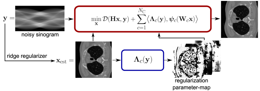
To obtain a regularization mask $\bm{\Lambda}$, we first compute an initial reconstruction ${\mathbf{x}}_{\mathrm{est}}$ from ${\mathbf{y}}$ based on (1) with an unadaptive (weakly) convex ridge regularizer $\mathcal{R}$ of the form (2). For this, we take the pre-trained models from [17], which are trained on 400 images of the BSD500 [37] training set for denoising with $\sigma\in[0,30/255]$. Note that the convolutions ${\mathbf{W}}$ and the potential $\psi$ remain fixed and are also used within the adaptive regularizer $\mathcal{R}_{{\mathbf{y}}}$. We solve problem (1) by performing accelerated gradient descent (AGD) with the modifications outlined in [17, Alg. 1]. Then, the obtained ${\mathbf{x}}_{\mathrm{est}}$ is plugged into a network $G\colon\mathbb{R}^{n}\to([0,1]^{n})^{N_{c}}$, which we choose as a lightweight variant of SwinIR [35]. To ensure the correct output range, we apply the algebraic function $x\mapsto x/\sqrt{x^{2}+1}$ to the last layer of $G$. We insert the obtained masks $\bm{\Lambda}_{c}({\mathbf{y}})$ into the regularizer architecture (3), for which we solve the associated variational problem (1) by performing AGD with starting point ${\mathbf{x}}_{\mathrm{est}}$. The whole computational pipeline is visualized in Figure 1.

Now, we detail the training of $\mathcal{R}_{{\mathbf{y}}}$, which includes learning the network $G$, the scalings $\alpha_{c}(\sigma)$ and the scalar $\mu$. Note that adapting the latter is necessary due to the range restriction of $G$. Let $\theta$ be the aggregated set of learnable parameters and let us denote $\mathcal{R}_{{\mathbf{y}},\sigma,\theta}=\mathcal{R}_{{\mathbf{y}},\sigma}$ for an explicit reference. We aim to learn $\theta$ in a supervised setting such that $\mathcal{R}_{{\mathbf{y}},\sigma,\theta}$ induces a good multi-noise-level Gaussian denoiser

$$D_{\sigma,\theta}({\mathbf{y}})=\mathrm{prox}_{\mathcal{R}_{{\mathbf{y}},\sigma,\theta}}({\mathbf{y}})=\operatorname*{arg\,min}_{{\mathbf{x}}\in\mathbb{R}^{n}}\frac{1}{2}\|{\mathbf{x}}-{\mathbf{y}}\|_{2}^{2}+\mathcal{R}_{{\mathbf{y}},\sigma,\theta}({\mathbf{x}}).$$ (71)

For this, we extract $M=110400$ patches $\{{\mathbf{x}}^{k}\}_{k=1}^{M}$ of size $80\times 80$ from the previously used 400 training images. The corresponding data is simulated as ${\mathbf{y}}^{k}={\mathbf{x}}^{k}+\sigma^{k}{\mathbf{n}}^{k}$ with Gaussian noise ${\mathbf{n}}^{k}\sim\mathcal{N}({\mathbf{0}},{\mathbf{I}})$ and standard deviations $\sigma^{k}$ uniformly drawn from $[0,30/255]$. This leads to the training problem

$$\operatorname*{arg\,min}_{\theta}\sum_{k=1}^{M}\mathbb{E}_{{\mathbf{n}}^{k}\sim\mathcal{N}({\mathbf{0}},{\mathbf{I}})}\mathbb{E}_{\sigma^{k}\sim\mathcal{U}([0,30/255])}\bigl{(}\bigl{\|}D_{\sigma^{k},\theta}({\mathbf{y}}^{k})-{\mathbf{x}}^{k}\bigr{\|}_{1}\bigr{)}.$$ (72)

During the training, the denoiser $D_{\sigma^{k},\theta}({\mathbf{y}}^{k})$ is evaluated using AGD and $\nabla_{\theta}D_{\sigma^{k},\theta}({\mathbf{y}}^{k})$ is computed using the implicit differentiation techniques detailed in [17]. We initialize the network parameters of $G$ randomly and $\alpha_{c}(\sigma)$ and $\mu$ are taken as in the pretrained ridge regularizer. Before training with all parameters, the NN $G$ is pre-trained for 2 epochs with $\sigma^{k}=25/255$ using the same procedure as for the full training described below. Then, the actual minimization of (72) is tackled using Adam [27] with batch size 32 and learning rate $\mathrm{lr}=$1\text{\cdot}{10}^{-4}$$ for the network $G$, $\mathrm{lr}=$5\text{\cdot}{10}^{-2}$$ for the scaling $\mu$ and $\mathrm{lr}=$5\text{\cdot}{10}^{-3}$$ for the spline $s_{\alpha_{c}}$. Moreover, we use a scheduler that reduces the learning rates linearly for the first 5 epochs such that the final ones are half the initial ones. In total, we train for 35 epochs. Then, we extract the model parameters $\theta$ for which the MSE on the validation set is the lowest. As for the ridge regularizers, we use Set12 [61] for validation.

When deploying the regularizer $\mathcal{R}_{{\mathbf{y}},\sigma}$ in the variational reconstruction model

$$\operatorname*{arg\,min}_{{\mathbf{x}}\in\mathbb{R}^{n}}\frac{1}{2}\|{\mathbf{H}}{\mathbf{x}}-{\mathbf{y}}\|_{2}^{2}+\lambda R_{{\mathbf{y}},\sigma}({\mathbf{x}}),$$ (73)

we need to specify the standard deviation $\sigma$ and the regularization strength $\lambda$. For image denoising, namely ${\mathbf{H}}=\text{Id}$, we use the actual standard deviation $\sigma$ of the noise model and set $\lambda=1$, which leads to a non-blind denoiser. For general inverse problems (or blind denoising), the standard deviation $\sigma$ is interpreted as a hyperparameter and tuned together with $\lambda$ on a small validation set (which is specified in the according subsections) using a grid search.

5 Experiments

In this section, we evaluate the proposed regularizer $\mathcal{R}_{{\mathbf{y}}}$ on various inverse problems. First, we investigate a simple denoising task. Then, we move to magnetic resonance imaging (MRI) in a single- and multi-coil setup in Section 5.2. In Section 5.3, we deploy $\mathcal{R}_{{\mathbf{y}}}$ for low-dose and limited-angle computed tomography (CT). Finally, we show results for the superresolution of material microstructures in Section 5.4. We quantitatively compare our method with established methods that can deal with very limited training data (a common setting for medical imaging or material sciences), namely with

• the total variation (TV) regularizer [51] as a well-known and widely used convex baseline;

• the Prox-DRUNet [25, 24] as one of the best-performing methods for convergent plug-and-play image-reconstruction [20, 58, 60]. For MRI and image superresolution, we deploy the DRS-PnP version described in [25], and the Prox-PnP-$\alpha$PGD described in [23] for CT. Here, one should keep in mind that the theoretical requirements are only imposed via regularization;

• the patchNR [1, 44], which performs particularly well in the regime of limited training data. This regularizer is non-convex and, apart from existence of a minimizer and an empirical convergence analysis, no other theoretical guarantees are known.

The reported quality metrics are the peak-signal-to-noise ratio (PSNR) and the structural similarity index measure (SSIM). Additionally, we provide the runtime of the methods for a single reconstruction. All experiments are implemented in PyTorch and the code is available online. The evaluations are performed on a NVIDIA GeForce RTX 2060 with 6GB GPU memory.

Method	BM3D	CRR	WCRR	Mask-CRR	Mask-WCRR	Prox-DRUNet
$\sigma=5/255$	37.54	36.96	37.63	37.70	37.80	37.98
$\sigma=15/255$	31.11	30.53	31.18	31.56	31.61	31.70
$\sigma=25/255$	28.60	28.08	28.68	29.13	29.13	29.18

Table 1: Denoising. Average PSNR on the BSD68 set. Best is bold and second best is underlined.

$\mathcal{R}({\mathbf{x}}_{\mathrm{gt}})$ (clean data)

$\mathcal{R}({\mathbf{y}})$ (noisy data)

$\mathcal{R}({\mathbf{x}}_{\mathrm{est}})$ (result)

$\mathcal{R}_{{\mathbf{y}}}({\mathbf{y}})$ (noisy data)

$\bm{\Lambda}({\mathbf{y}})$ (average mask)

Figure 2: Pixel-wise cost $\mathcal{R}({\mathbf{x}})=\sum_{c}\bm{\psi}_{c}({\mathbf{W}}_{c}{\mathbf{x}})$ for images ${\mathbf{x}}\in\{{\mathbf{x}}_{\mathrm{gt}},{\mathbf{y}},{\mathbf{x}}_{\mathrm{est}}\}$. Next, we visualize the data-dependent cost $\mathcal{R}_{{\mathbf{y}}}({\mathbf{x}})=\sum_{c}\langle\bm{\Lambda}({\mathbf{y}}),\bm{\psi}_{c}({\mathbf{W}}_{c}{\mathbf{x}})\rangle$ and the pixel-wise average mask $\bm{\Lambda}({\mathbf{y}})$.

Original

Noisy

BM3D

CRR

WCRR

Mask-CRR

Mask-WCRR

Prox-DRUNet

Figure 3: Denoising of the castle image for $\sigma=25/255$. The zoomed area is marked by a white box.

5.1 Denoising

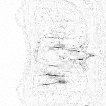
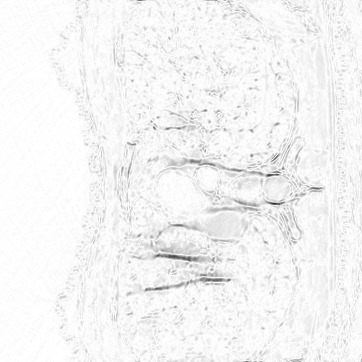
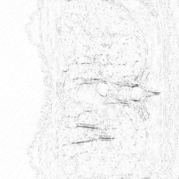
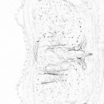
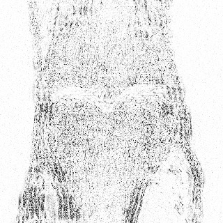
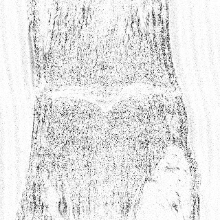
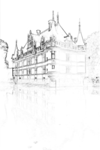
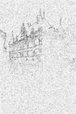
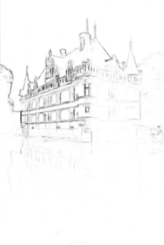
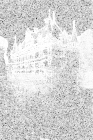
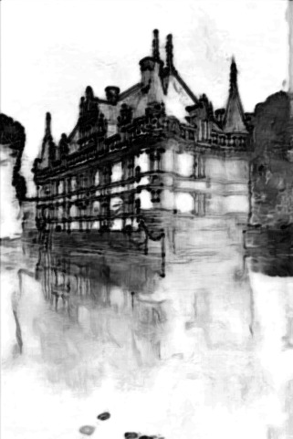
First, we evaluate the methods for denoising on the BSD68 dataset [37]. Since the standard deviation $\sigma$ is used as input for all methods, the task is non-blind. The quantitative results for different $\sigma$ are given in Table 1, where we also include the popular BM3D denoiser [8]. In particular, we observe that the mask $\bm{\Lambda}$ improves both the CRR and the WCRR. This can be explained by the damped filter response to structure. An illustration of this behavior for the CRR is given in Figure 3, where we visualize the pixel-wise cost of the regularizers; for WCRR, the visualizations would look similarly. The values of $\bm{\Lambda}$ are smaller (black) in structured areas and higher (white) in constant ones, which prevents oversmoothing. Secondly, we observe that, after applying $\bm{\Lambda}$, the two regularizers CRR and WCRR perform similarly. This is in contrast to the baseline setting, where the WCRR clearly outperforms the CRR. A qualitative result for the castle image and $\sigma=25/255$ is given in Figure 3. While the differences between the results with CRR and WCRR are very pronounced, the addition of $\bm{\Lambda}$ leads to visually similar results with some small differences: Since the top of the spire is still contained in the CRR result, the structure-detecting mask $\bm{\Lambda}$ enables us to recover most of it. In contrast, it is already lost for the WCRR result, and $\bm{\Lambda}$ cannot help anymore. In particular, we observe that the mask $\bm{\Lambda}$ can only enhance structure that is present in ${\mathbf{x}}_{\text{est}}$.

5.2 Magnetic Resonance Imaging

	4-fold single coil
	PD	PDFS	PD	PDFS	time
Zero-Filled	27.40 $\pm$ 2.41	29.68 $\pm$ 1.58	0.714 $\pm$ 0.053	0.719 $\pm$ 0.049	0.02s
TV	32.30 $\pm$ 2.62	32.56 $\pm$ 1.78	0.827 $\pm$ 0.052	0.775 $\pm$ 0.061	4s
CRR	33.39 $\pm$ 2.65	33.44 $\pm$ 1.82	0.870 $\pm$ 0.042	0.824 $\pm$ 0.050	24s
WCRR	35.74 $\pm$ 2.51	34.60 $\pm$ 1.96	0.897 $\pm$ 0.039	0.837 $\pm$ 0.053	20s
Mask-CRR	35.86 $\pm$ 2.49	34.60 $\pm$ 1.97	0.903 $\pm$ 0.036	0.838 $\pm$ 0.051	38s
Mask-WCRR	36.19 $\pm$ 2.53	34.68 $\pm$ 1.98	0.904 $\pm$ 0.038	0.840 $\pm$ 0.051	37s
Prox-DRUNet DRS	36.14 $\pm$ 2.52	35.05 $\pm$ 1.97	0.900 $\pm$ 0.039	0.847 $\pm$ 0.048	625s
patchNR	35.80 $\pm$ 2.84	34.26 $\pm$ 2.06	0.895 $\pm$ 0.043	0.830 $\pm$ 0.057	116s
	8-fold multi coil
	PD	PDFS	PD	PDFS	time
Zero-Filled	23.80 $\pm$ 2.34	27.19 $\pm$ 1.62	0.628 $\pm$ 0.061	0.649 $\pm$ 0.065	0.02s
TV	31.14 $\pm$ 3.14	32.12 $\pm$ 2.15	0.807 $\pm$ 0.060	0.769 $\pm$ 0.070	16s
CRR	33.90 $\pm$ 2.81	34.28 $\pm$ 2.08	0.875 $\pm$ 0.038	0.847 $\pm$ 0.049	27s
WCRR	35.50 $\pm$ 2.40	35.12 $\pm$ 2.13	0.894 $\pm$ 0.032	0.855 $\pm$ 0.052	27s
Mask-CRR	35.73 $\pm$ 2.49	35.20 $\pm$ 2.11	0.900 $\pm$ 0.031	0.858 $\pm$ 0.049	38s
Mask-WCRR	36.00 $\pm$ 2.36	35.23 $\pm$ 2.12	0.902 $\pm$ 0.030	0.858 $\pm$ 0.050	38s
Prox-DRUNet DRS	35.81 $\pm$ 2.36	35.13 $\pm$ 2.14	0.894 $\pm$ 0.031	0.857 $\pm$ 0.052	625s
patchNR	35.35 $\pm$ 3.09	34.84 $\pm$ 2.15	0.888 $\pm$ 0.042	0.849 $\pm$ 0.054	119s

Table 2: MRI. Average metrics and standard deviations evaluated on 50 images of the fastMRI dataset. Best is bold and second best is underlined.

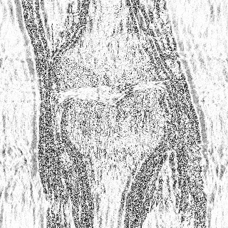
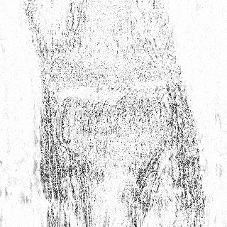
Next, we investigate the single- and 15-coil MRI setups detailed in [16, 41], where ${\mathbf{H}}$ essentially corresponds to a subsampled Fourier transform. For both setups, we have to reconstruct proton-density-weighted knee images from the fastMRI dataset [28] with (PDFS) and without (PD) fat suppression. To generate ground truth images for the four tasks, we use the fully sampled k-space measurements. The data subsampling ratio is determined by the acceleration factor $M_{\text{acc}}$, i.e., we keep $1/M_{\text{acc}}$ of the columns in the k-space. For the single-coil setup, we generate the measurements by a $4$-fold ($M_{\text{acc}}=4$) subsampling of the k-space data. In the 15-coil setup, we apply $8$-fold ($M_{\text{acc}}=8$) subsampling to the Fourier transforms of the ground-truth images multiplied by the respective sensitivity maps. For this, we use the BART [56] implementation of the ESPIRiT algorithm [55]. The data is then corrupted with additive Gaussian noise of standard deviation $\sigma=$2\text{\cdot}{10}^{-3}$$ to the real and imaginary part. Thus, from a Bayesian viewpoint, the negative log-likelihood can be written as

$$-\log(p_{{\mathbf{Y}}|{\mathbf{X}}={\mathbf{x}}}({\mathbf{y}}))\propto\frac{1}{2\sigma^{2}}\|{\mathbf{H}}{\mathbf{x}}-{\mathbf{y}}\|^{2}.$$ (74)

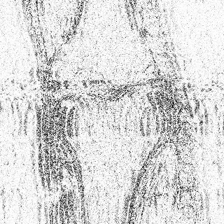
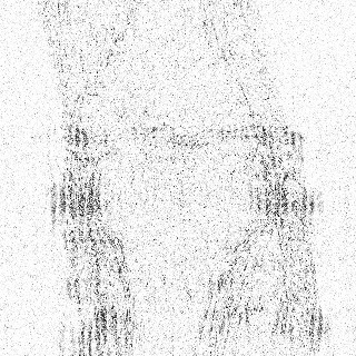
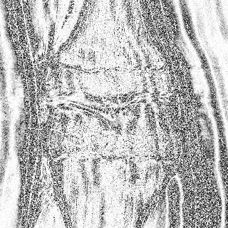
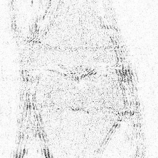
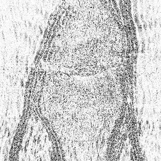
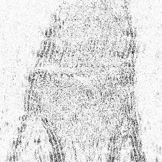
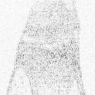
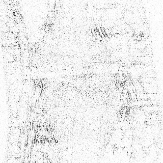
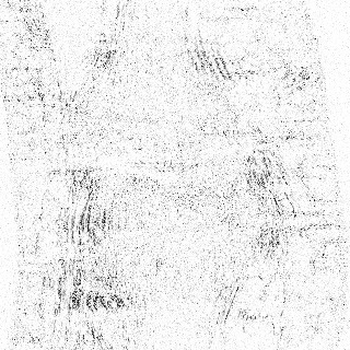
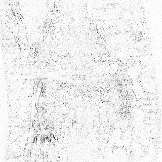
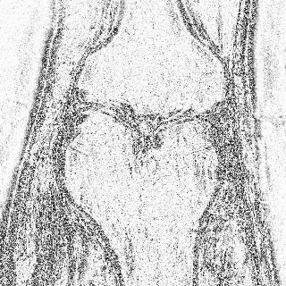
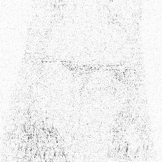
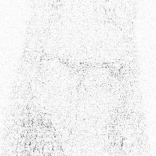
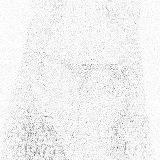
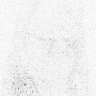
For each task, we use ten validation images to determine the hyperparameters $\lambda$ and $\sigma$. Additionally, we finetune $\bm{\Lambda}$ for 30 epochs on these images, and train the patchNR on them. The quantitative results on a test set of 50 images are reported in Table 2. Moreover, qualitative results are given in Figures 5 and 5. Again, the performance of CRR and WCRR increases with the addition of $\bm{\Lambda}$. In particular, the Mask-CRR improves significantly for all cases. Overall, the Mask-WCRR performs best. Similar reconstruction quality is achieved with the Prox-DRUNet. Its drawback is that it takes 15 times longer than the Mask-WCRR. For this MRI task, the patchNR struggles to reconstruct the finer structures and performs worse than the other methods. More reconstructions are given in Appendix A.

GT

Zero-filled

CRR

WCRR

CRR-Mask

WCRR-Mask

Prox-DRUNet

patchNR

Figure 4: 4-fold single-coil MRI without fat suppression. The zoomed-in part is marked with a white box. Top: full image; middle: zoomed-in part; bottom: error.

GT

Zero-filled

CRR

WCRR

CRR-Mask

WCRR-Mask

Prox-DRUNet

patchNR

GT

Zero-filled

CRR

WCRR

CRR-Mask

WCRR-Mask

Prox-DRUNet

patchNR

Figure 5: 8-fold multi-coil MRI with (bottom) and without (top) fat suppression. The zoomed-in part is marked with a white box. Top: full image; middle: zoomed-in part; bottom: error.

5.3 Computed Tomography

For this example, ${\mathbf{H}}$ is a discretized linear Radon transform and the noise is modeled by a Poisson distribution. More precisely, the corrupted entries of the measurement ${\mathbf{y}}$ are given by

$${\mathbf{y}}=-\frac{1}{\mu}\log\Bigl{(}\frac{\tilde{{\mathbf{y}}}}{N_{0}}\Bigr{)},\quad\tilde{{\mathbf{y}}}\sim\mathrm{Pois}\bigl{(}N_{0}\exp(-{\mathbf{H}}{\mathbf{x}}\mu)\bigr{)},$$ (75)

where $\mathrm{Pois}(\lambda)$ is the Poisson distribution with mean $\lambda$, $N_{0}=4096$ is the mean photon count per detector bin without attenuation, and $\mu=81.35858$ is a normalization constant. The ground truth images from the LoDoPaB dataset [33] have a resolution of $362\times 362$ and the measurements are simulated with a parallel beam geometry with 513 equidistant detector bins and 1000 equidistant angles between $0$ and $\pi$. By computing $-\log p_{{\mathbf{Y}}|{\mathbf{X}}={\mathbf{x}}}({\mathbf{y}})$ and omitting summands depending only on ${\mathbf{y}}$, we arrive at the data fidelity

$$\mathcal{D}({\mathbf{H}}{\mathbf{x}},{\mathbf{y}})=\sum_{i=1}^{m}\exp\left(-({\mathbf{H}}{\mathbf{x}})_{i}\mu\right)N_{0}+\exp\left(-\mu{\mathbf{y}}_{i}\right)N_{0}\bigl{(}\mu({\mathbf{H}}{\mathbf{x}})_{i}-\log(N_{0})\bigr{)}.$$ (76)

To get a fair comparison with the patchNR, which is trained on 6 ground truth images of the training set, we finetune the parameters of $\bm{\Lambda}$ for 30 epochs on the same images. Once finetuned, we use $\mathcal{R}_{{\mathbf{y}}}$ for both low-dose and limited-angle CT. Moreover, the parameters $\lambda$ and $\sigma$ are tuned for all methods using the coarse-to-fine grid search from [16] on the same single validation image used for the patchNR.

Low-Dose CT

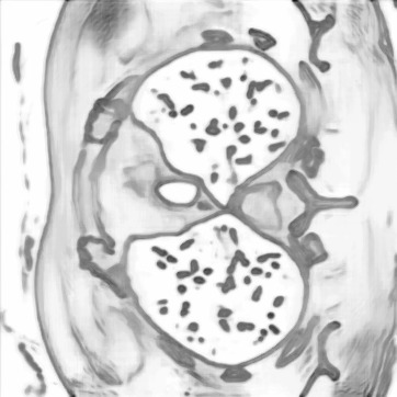
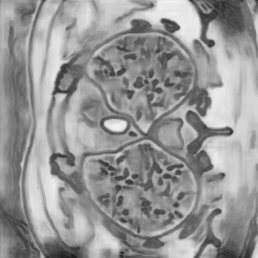
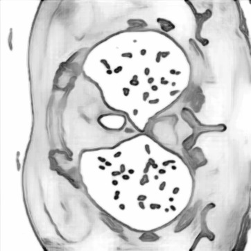
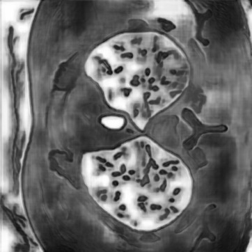
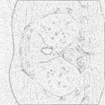
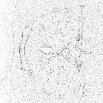
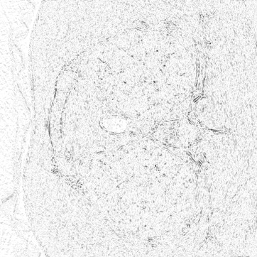
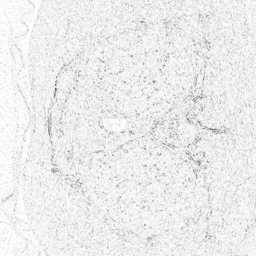
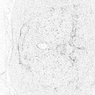
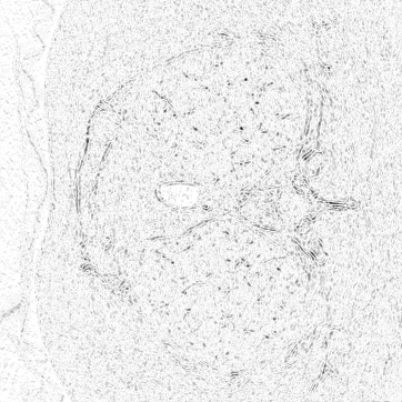
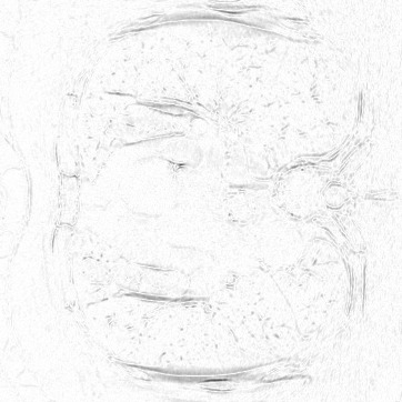
In Table 3, we report quantitative results for the first 100 test images of the LoDoPaB test split. Again, the addition of $\bm{\Lambda}$ leads to a significant improvement of the metrics. In particular, see Figure 8, the mask generation process behaves robust to the task shift. In Figure 8, we provide several reconstructions, including the filtered back-projection (FBP) [47] as a baseline. The squared difference to the ground truth is taken into account as the error. For better visibility, the differences are rescaled with a square root. While the WCRR outperforms CRR both visually and in terms of the metrics, the data-dependent counterparts behave very similar. Despite these quality improvements, the patchNR still leads to visually more appealing results. Note that for the data fidelity term (76), no closed form of its proximal operator exists. Therefore, the DRS-PnP algorithm becomes impractical and we use a relaxed version of the PGD-PnP [23] instead. There, to meet the convergence criteria, the learned denoiser needs to be relaxed. Within this setting, we did not achieve competitive results and only report the obtained ones for the sake of completeness. More reconstructions are given in Appendix A.

	low-dose CT			limited-angle CT
	PSNR	SSIM	time	PSNR	SSIM	time
FBP	30.37 $\pm$ 2.95	0.739 $\pm$ 0.141	0.03s	21.96 $\pm$ 2.25	0.531 $\pm$ 0.097	0.03s
TV	32.87 $\pm$ 3.79	0.796 $\pm$ 0.151	12s	29.40 $\pm$ 2.73	0.756 $\pm$ 0.151	16s
CRR	34.37 $\pm$ 4.20	0.818 $\pm$ 0.154	16s	31.75 $\pm$ 3.24	0.792$\pm$ 0.155	18s
WCRR	34.87 $\pm$ 4.40	0.822$\pm$ 0.156	19s	32.54 $\pm$ 3.46	0.797 $\pm$ 0.157	19s
Mask-CRR	35.14 $\pm$ 4.53	0.826 $\pm$ 0.154	34s	33.02 $\pm$ 3.61	0.805 $\pm$ 0.156	38s
Mask-WCRR	35.07 $\pm$ 4.54	0.824 $\pm$ 0.157	32s	33.09 $\pm$ 3.62	0.805 $\pm$ 0.156	30s
Prox-DRUNet-$\alpha$PGD	34.23 $\pm$ 4.32	0.811 $\pm$ 0.154	593s	31.04 $\pm$ 3.23	0.771 $\pm$ 0.157	593s
patchNR	35.19 $\pm$ 4.52	0.829 $\pm$ 0.152	48s	33.20 $\pm$ 3.55	0.811 $\pm$ 0.151	486s

Table 3: CT. Average metrics and standard deviations for the first 100 images of the LoDoPaB test set. Best is bold and second best is underlined.

Mask-CRR

Mask-WCRR

Mask-CRR

Mask-WCRR

Figure 6: Masks $\bm{\Lambda}$ for CRR and WCRR in the low-dose (left) and limited-angle CT (right) setting.

GT

FBP

CRR

WCRR

Mask-CRR

Mask-WCRR

Prox-DRUNet

patchNR

Figure 7: Low-dose CT. The zoomed-in part is marked with a white box. Top: full image; middle: zoomed-in part; bottom: error.

GT

FBP

CRR

WCRR

Mask-CRR

Mask-WCRR

Prox-DRUNet

patchNR

Figure 8: Limited-angle CT. The zoomed-in part is marked with a white box. Second: full image; top and third: zoomed-in part; bottom: error.

Limited-Angle CT

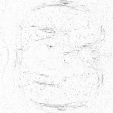
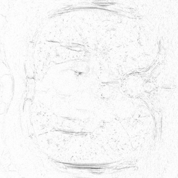
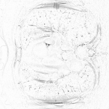
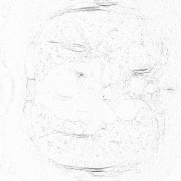
Here, we remove the first and last 100 angles from the data, which corresponds to $36^{\circ}$ out of $180^{\circ}$. Several reconstructions and quantitative metrics are given in Figure 8 and Table 3, respectively. This task is much harder than the previous one, which becomes most evident when inspecting the FBP reconstruction. Overall, the performance comparison between the methods turns out similar as before. Interestingly, the performance boost attributed to the masks becomes even higher for this setup. In Figure 8, we can see that the masks remain reasonable despite the large amount of missing data. While the CRR masks look similar for both CT setups, the WCRR ones are considerably different. This is a bit surprising and a direction for further investigations. More reconstructions are available in Appendix A.

5.4 Image Superresolution

Here, we consider the superresolution of microstructures in a composite (“SiC Diamonds”) obtained by microwave sintering of silicon and diamonds, which was previously also considered in [19, 1]. The dataset consists of 2D slices of size $600\times 600$. These are extracted from a 3D image of size $2560\times 2560\times 2120$, which was acquired by microcomputed tomography at the SLS beamline TOMCAT. The operator ${\mathbf{H}}$ is a convolution with a $16\times 16$ Gaussian kernel with standard deviation 2 and stride 4, namely with 4-fold subsampling. The data is simulated by applying ${\mathbf{H}}$ to the groundtruth and adding Gaussian noise with $\sigma=0.01$, which leads to the same $\mathcal{D}$ as in Section 5.2.

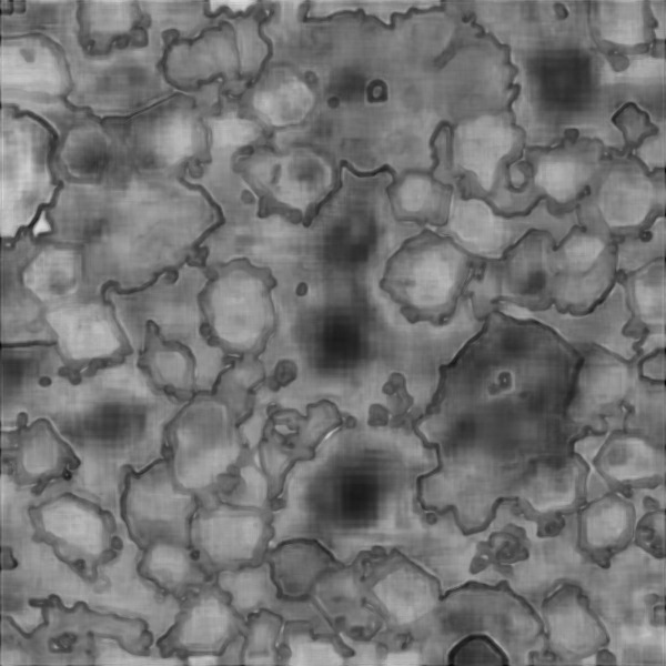
While the patchNR is trained on a single reference image of size $600\times 600$, the other methods are not adapted to this dataset and task. For all methods, we use a single validation image to determine the hyperparameters $\lambda$ and $\sigma$. In Figure 10, we provide visual results and in Figure 10 we show the regularization masks of Mask-CRR and Mask-WCRR. Note that the sparsity priors CRR and WCRR suffer from a significant blur in their reconstruction, particularly for the small regions between the structures. Here, the addition of $\bm{\Lambda}$ leads to some improvement. Note that the contrast in $\bm{\Lambda}$ is much higher for the CRR compared to the WCRR. For the latter, the penalization of structure is already considerably dampened by the $1$-weakly convex potentials and a less pronounced mask seems to suffice. While the results of Mask-CRR, Mask-WCRR and Prox-DRUNet are sharper, they still do not match the patchNR. In particular, this method is the only one that reconstructs the tiny bright structure in the bottom of the zoomed-in part. These observations are confirmed by the quantitative results in Table 4. Given that the other priors are not tailored to this very particular data, the superiority of the patchNR is not too surprising. More superresolution results are included in Appendix A.

	SiC
	PSNR	SSIM	time
Bicubic	25.63 $\pm$ 0.56	0.699$\pm$ 0.012	0.0002s
TV	26.14 $\pm$ 0.61	0.710 $\pm$ 0.018	11s
CRR	27.83$\pm$ 0.52	0.772 $\pm$ 0.008	38s
WCRR	28.17$\pm$ 0.54	0.788 $\pm$ 0.010	38s
Mask-CRR	28.21 $\pm$ 0.55	0.788 $\pm$ 0.010	45s
Mask-WCRR	28.27 $\pm$ 0.55	0.790 $\pm$ 0.010	45s
Prox-DRUNet DRS	28.21 $\pm$ 0.52	0.789 $\pm$ 0.010	652s
patchNR	28.53 $\pm$ 0.49	0.780 $\pm$ 0.008	151s

Table 4: Superresolution of SiC. Averaged metrics and standard deviations evaluated on 100 test images. Best is bold and second best is underlined.

HR

LR

CRR

WCRR

Mask-CRR

Mask-WCRR

Prox-DRUNet

patchNR

Figure 9: Superresolution of material microstructures. The zoomed-in part is marked with a white box. Top: full image; bottom: zoomed-in part.

Mask-CRR

Mask-WCRR

Figure 10: Masks $\bm{\Lambda}$ for image superresolution of material‘s microstructures.

6 Conclusion

In this paper, we established theoretical guarantees for ridge-based regularization. Here, the (rather uncommon) data-dependence of the regularizer $\mathcal{R}_{{\mathbf{y}}}$ made a new analysis necessary. So far, there is a discrepancy regarding the strength of our results between the CRR and the WCRR setting, which opens possibilities for future work. For now, given their similar experimental performance, we suggest to use the Mask-CRR instead of the Mask-WCRR. Additionally, it would be interesting to work out conditions under which a unique critical point exists, similar as in compressed sensing. Then, our results directly translate into the stronger notion of classical Lipschitz continuity.

From a practical perspective, our approach can be extended into several directions. Since $\mathcal{R}_{{\mathbf{y}}}$ induces a probability distribution, we can apply it for uncertainty quantification based on invertible architectures [2, 11, 18] or Langevin methods as done for the patchNR in [5]. Throughout this paper, we trained both the mask $\bm{\Lambda}$ and the baseline regularizer $\mathcal{R}$ for denoising of natural images. As a result, our model is extremely flexible, and we can apply it to any inverse problem by simply adjusting the regularization strength $\lambda$ and the noise level $\sigma$ without any further training. Still, if we have knowledge about the operator ${\mathbf{H}}$, the noise model or sufficiently many task specific training images, we can train $\mathcal{R}_{{\mathbf{y}}}$ for the specific setting. In particular, we can get rid of a first preprocessing step for the regularization parameter map and instead use the observation directly. This likely improves the performance and makes our approach, besides its theoretical guarantees, even more relevant to practical applications.

Appendix A Reconstruction Examples

Here, we provide additional qualitative results for the numerical examples from Section 5, see Figures 11 and 12 for low-dose and limited-angle CT, respectively, and Figures 13 to 16 for the MRI experiments, and Figure 17 for the superresolution example.

GT

FBP

CRR

WCRR

Mask-CRR

Mask-WCRR

Prox-DRUNet

patchNR

GT

FBP

CRR

WCRR

Mask-CRR

Mask-WCRR

Prox-DRUNet

patchNR

GT

FBP

CRR

WCRR

Mask-CRR

Mask-WCRR

Prox-DRUNet

patchNR

Figure 11: Low-dose CT. The zoomed-in part is marked with a white box. Top: full image; middle: zoomed-in part; bottom: error.

GT

FBP

CRR

WCRR

Mask-CRR

Mask-WCRR

Prox-DRUNet

patchNR

GT

FBP

CRR

WCRR

Mask-CRR

Mask-WCRR

Prox-DRUNet

patchNR

GT

FBP

CRR

WCRR

Mask-CRR

Mask-WCRR

Prox-DRUNet

patchNR

Figure 12: Limited-angle CT. The zoomed-in part is marked with a white box. Top: full image; middle: zoomed-in part; bottom: error.

GT

Zero-filled

CRR

WCRR

CRR-Mask

WCRR-Mask

Prox-DRUNet

patchNR

GT

Zero-filled

CRR

WCRR

CRR-Mask

WCRR-Mask

Prox-DRUNet

patchNR

GT

Zero-filled

CRR

WCRR

CRR-Mask

WCRR-Mask

Prox-DRUNet

patchNR

Figure 13: 4-fold single-coil MRI without fat suppression. The zoomed-in part is marked with a white box. Top: full image; middle: zoomed-in part; bottom: error.

GT

Zero-filled

CRR

WCRR

CRR-Mask

WCRR-Mask

Prox-DRUNet

patchNR

GT

Zero-filled

CRR

WCRR

CRR-Mask

WCRR-Mask

Prox-DRUNet

patchNR

GT

Zero-filled

CRR

WCRR

CRR-Mask

WCRR-Mask

Prox-DRUNet

patchNR

Figure 14: 4-fold single-coil MRI with fat suppression. The zoomed-in part is marked with a white box. Top: full image; middle: zoomed-in part; bottom: error.

GT

Zero-filled

CRR

WCRR

CRR-Mask

WCRR-Mask

Prox-DRUNet

patchNR

GT

Zero-filled

CRR

WCRR

CRR-Mask

WCRR-Mask

Prox-DRUNet

patchNR

GT

Zero-filled

CRR

WCRR

CRR-Mask

WCRR-Mask

Prox-DRUNet

patchNR

Figure 15: 8-fold multi-coil MRI without fat suppression. The zoomed-in part is marked with a white box. Top: full image; middle: zoomed-in part; bottom: error.

GT

Zero-filled

CRR

WCRR

CRR-Mask

WCRR-Mask

Prox-DRUNet

patchNR

GT

Zero-filled

CRR

WCRR

CRR-Mask

WCRR-Mask

Prox-DRUNet

patchNR

GT

Zero-filled

CRR

WCRR

CRR-Mask

WCRR-Mask

Prox-DRUNet

patchNR

Figure 16: 8-fold multi-coil MRI with fat suppression. The zoomed-in part is marked with a white box. Top: full image; middle: zoomed-in part; bottom: error.

HR

LR

CRR

WCRR

Mask-CRR

Mask-WCRR

Prox-DRUNet

patchNR

HR

LR

CRR

WCRR

Mask-CRR

Mask-WCRR

Prox-DRUNet

patchNR

HR

LR

CRR

WCRR

Mask-CRR

Mask-WCRR

Prox-DRUNet

patchNR

Figure 17: Superresolution of material microstructures. The zoomed-in part is marked with a white box. Top: full image; bottom: zoomed-in part.

References

- [1] F. Altekrüger, A. Denker, P. Hagemann, J. Hertrich, P. Maass, and G. Steidl. PatchNR: Learning from very few images by patch normalizing flow regularization. Inverse Problems, 39(6):064006, 2023.
- [2] L. Ardizzone, J. Kruse, C. Rother, and U. Köthe. Analyzing inverse problems with invertible neural networks. In International Conference on Learning Representations, 2019.
- [3] J. Bolte and E. Pauwels. Conservative set valued fields, automatic differentiation, stochastic gradient methods and deep learning. Mathematical Programming, 188(1):19–51, 2021.
- [4] J. Bolte, E. Pauwels, and A. Silveti-Falls. Differentiating nonsmooth solutions to parametric monotone inclusion problems. SIAM Journal on Optimization, 34(1):71–97, 2024.
- [5] Z. Cai, J. Tang, S. Mukherjee, J. Li, C.-B. Schönlieb, and X. Zhang. NF-ULA: normalizing flow-based unadjusted Langevin algorithm for imaging inverse problems. SIAM Journal on Imaging Sciences, 17(2):820–860, 2024.
- [6] F. H. Clarke. Optimization and Nonsmooth Analysis, volume 5 of Classics in Applied Mathematics. SIAM, Philadelphia, PA, 1990.
- [7] N. D. Cuong and A. Y. Kruger. Uniform regularity of set-valued mappings and stability of implicit multifunctions. Journal of Nonsmooth Analysis and Optimization, 2:6599, 2021.
- [8] K. Dabov, A. Foi, V. Katkovnik, and K. Egiazarian. Image denoising by sparse 3-D transform-domain collaborative filtering. IEEE Transactions on Image Processing, 16(8):2080–2095, 2007.
- [9] A. Daniilidis and J. C. H. Pang. Continuity and differentiability of set-valued maps revisited in the light of tame geometry. Journal of the London Mathematical Society. Second Series, 83(3):637–658, 2011.
- [10] P. del Aguila Pla, S. Neumayer, and M. Unser. Stability of image-reconstruction algorithms. IEEE Transactions on Computional Imaging, 9:1–12, 2023.
- [11] L. Dinh, J. Sohl-Dickstein, and S. Bengio. Density estimation using real NVP. In International Conference on Learning Representations, 2017.
- [12] Y. Dong and C.-B. Schönlieb. Tomographic reconstruction with spatially varying parameter selection. Inverse Problems, 36(5):054002, 2020.
- [13] D. L. Donoho. Compressed sensing. IEEE Transactions on Information Theory, 52(4):1289–1306, 2006.
- [14] A. L. Dontchev and R. T. Rockafellar. Implicit Functions and Solution Mappings. Springer Monographs in Mathematics. Springer, Dordrecht, 2009.
- [15] H. Gfrerer and J. V. Outrata. On Lipschitzian properties of implicit multifunctions. SIAM Journal on Optimization, 26(4):2160–2189, 2016.
- [16] A. Goujon, S. Neumayer, P. Bohra, S. Ducotterd, and M. Unser. A neural-network-based convex regularizer for inverse problems. IEEE Transactions on Computational Imaging, 9:781–795, 2023.
- [17] A. Goujon, S. Neumayer, and M. Unser. Learning weakly convex regularizers for convergent image-reconstruction algorithms. SIAM Journal on Imaging Sciences, 17(1):91–115, 2024.
- [18] P. Hagemann, J. Hertrich, and G. Steidl. Stochastic normalizing flows for inverse problems: a Markov Chains viewpoint. SIAM/ASA Journal on Uncertainty Quantification, 10(3):1162–1190, 2022.
- [19] J. Hertrich, A. Houdard, and C. Redenbach. Wasserstein patch prior for image superresolution. IEEE Transactions on Computational Imaging, 8:693–704, 2022.
- [20] J. Hertrich, S. Neumayer, and G. Steidl. Convolutional proximal neural networks and Plug-and-Play algorithms. Linear Algebra and its Applications, 631:203–234, 2021.
- [21] M. Hintermüller, K. Papafitsoros, and C. N. Rautenberg. Analytical aspects of spatially adapted total variation regularisation. Journal of Mathematical Analysis and Applications, 454(2):891–935, 2017.
- [22] A. J. Hoffman. On approximate solutions of systems of linear inequalities. Journal of Research of the National Bureau of Standards, 49:263–265, 1952.
- [23] S. Hurault, A. Chambolle, A. Leclaire, and N. Papadakis. A relaxed proximal gradient descent algorithm for convergent Plug-and-Play with proximal denoiser. In International Conference on Scale Space and Variational Methods in Computer Vision, pages 379–392. Springer, 2023.
- [24] S. Hurault, A. Leclaire, and N. Papadakis. Gradient step denoiser for convergent Plug-and-Play. In International Conference on Learning Representations, 2022.
- [25] S. Hurault, A. Leclaire, and N. Papadakis. Proximal denoiser for convergent Plug-and-Play optimization with nonconvex regularization. In K. Chaudhuri, S. Jegelka, L. Song, C. Szepesvari, G. Niu, and S. Sabato, editors, Proceedings of the 39th International Conference on Machine Learning, pages 9483–9505. PMLR, 2022.
- [26] A. D. Ioffe. Variational Analysis of Regular Mappings. Springer Monographs in Mathematics. Springer, Cham, 2017.
- [27] D. P. Kingma and J. Ba. Adam: A method for stochastic optimization. In International Conference on Learning Representations, 2015.
- [28] F. Knoll, J. Zbontar, A. Sriram, M. J. Muckley, M. Bruno, A. Defazio, M. Parente, K. J. Geras, J. Katsnelson, H. Chandarana, Z. Zhang, M. Drozdzalv, A. Romero, M. Rabbat, P. Vincent, J. Pinkerton, D. Wang, N. Yakubova, E. Owens, C. L. Zitnick, M. P. Recht, D. K. Sodickson, and Y. W. Lui. fastMRI: A publicly available raw k-space and DICOM dataset of knee images for accelerated MR image reconstruction using machine learning. Radiology: Artificial Intelligence, 2(1):e190007, 2020.
- [29] E. Kobler, A. Effland, K. Kunisch, and T. Pock. Total deep variation for linear inverse problems. In Conference on Computer Vision and Pattern Recognition, pages 7549–7558, 2020.
- [30] E. Kobler, A. Effland, K. Kunisch, and T. Pock. Total deep variation: A stable regularization method for inverse problems. IEEE Transactions on Pattern Analysis and Machine Intelligence, 44(12):9163–9180, 2021.
- [31] A. Kofler, F. Altekrüger, F. Antarou Ba, C. Kolbitsch, E. Papoutsellis, D. Schote, C. Sirotenko, F. F. Zimmermann, and K. Papafitsoros. Learning regularization parameter-maps for variational image reconstruction using deep neural networks and algorithm unrolling. SIAM Journal on Imaging Sciences, 16(4):2202–2246, 2023.
- [32] S. Lefkimmiatis and I. S. Koshelev. Learning sparse and low-rank priors for image recovery via iterative reweighted least squares minimization. In International Conference on Learning Representations, 2023.
- [33] J. Leuschner, M. Schmidt, D. O. Baguer, and P. Maass. LoDoPaB-CT, a benchmark dataset for low-dose computed tomography reconstruction. Scientific Data, 8(109), 2021.
- [34] H. Li, J. Schwab, S. Antholzer, and M. Haltmeier. NETT: Solving inverse problems with deep neural networks. Inverse Problems, 36(6):065005, 2020.
- [35] J. Liang, J. Cao, G. Sun, K. Zhang, L. Van Gool, and R. Timofte. SwinIR: Image restoration using swin transformer. In IEEE/CVF International Conference on Computer Vision Workshops, pages 1833–1844, 2021.
- [36] S. Lunz, O. Öktem, and C.-B. Schönlieb. Adversarial regularizers in inverse problems. In Advances in Neural Information Processing Systems, volume 31, 2018.
- [37] D. Martin, C. Fowlkes, D. Tal, and J. Malik. A database of human segmented natural images and its application to evaluating segmentation algorithms and measuring ecological statistics. IEEE International Conference on Computer Vision, pages 416–423, 2001.
- [38] M. T. McCann and M. Unser. Biomedical image reconstruction: From the foundations to deep neural networks. Foundations and Trends® in Signal Processing, 13(3):283–359, 2019.
- [39] S. Mukherjee, S. Dittmer, Z. Shumaylov, S. Lunz, O. Öktem, and C.-B. Schönlieb. Learned convex regularizers for inverse problems. arXiv preprint arXiv:2008.02839, 2020.
- [40] S. Mukherjee, A. Hauptmann, O. Öktem, M. Pereyra, and C.-B. Schönlieb. Learned reconstruction methods with convergence guarantees: A survey of concepts and applications. IEEE Signal Process. Mag., 40(1):164–182, 2023.
- [41] S. Neumayer, M. Pourya, A. Goujon, and M. Unser. Boosting weakly convex ridge regularizers with spatial adaptivity. In NeurIPS Workshop on Deep Learning and Inverse Problems, 2023.
- [42] D. Obmann and M. Haltmeier. Convergence analysis of critical point regularization with non-convex regularizers. Inverse Problems, 39(8):085004, 2023.
- [43] J. Peña, J. C. Vera, and L. F. Zuluaga. New characterizations of Hoffman constants for systems of linear constraints. Mathematical Programming, 187(1-2):79–109, 2021.
- [44] M. Piening, F. Altekrüger, J. Hertrich, P. Hagemann, A. Walther, and G. Steidl. Learning from small data sets: Patch-based regularizers in inverse problems for image reconstruction. arXiv preprint arXiv:2312.16611, 2023.
- [45] M. Pragliola, L. Calatroni, A. Lanza, and F. Sgallari. On and beyond total variation regularization in imaging: The role of space variance. SIAM Review, 65(3):601–685, 2023.
- [46] J. Prost, A. Houdard, A. Almansa, and N. Papadakis. Learning local regularization for variational image restoration. In International Conference on Scale Space and Variational Methods in Computer Vision, pages 358–370. Springer, 2021.
- [47] J. Radon. On the determination of functions from their integral values along certain manifolds. IEEE Transactions on Medical Imaging, 5(4):170–176, 1986.
- [48] A. Ribes and F. Schmitt. Linear inverse problems in imaging. IEEE Signal Processing Magazine, 25(4):84–99, 2008.
- [49] R. T. Rockafellar and R. J.-B. Wets. Variational Analysis, volume 317 of Grundlehren der Mathematischen Wissenschaften. Springer-Verlag, Berlin, 1998.
- [50] S. Roth and M. J. Black. Fields of experts. International Journal of Computer Vision, 82(2):205–229, 2009.
- [51] L. I. Rudin, S. Osher, and E. Fatemi. Nonlinear total variation based noise removal algorithms. Physica D: Nonlinear Phenomena, 60(1-4):259–268, 1992.
- [52] O. Scherzer, M. Grasmair, H. Grossauer, M. Haltmeier, and F. Lenzen. Variational Methods in Imaging, volume 167 of Applied Mathematical Sciences. Springer, 2009.
- [53] Z. Shumaylov, J. Budd, S. Mukherjee, and C.-B. Schönlieb. Weakly convex regularisers for inverse problems: Convergence of critical points and primal-dual optimisation. arXiv preprint arXiv:2402.01052, 2024.
- [54] A. N. Tikhonov. Solution of incorrectly formulated problems and the regularization method. Soviet Mathematics, 4:1035–1038, 1963.
- [55] M. Uecker, P. Lai, M. J. Murphy, P. Virtue, M. Elad, J. M. Pauly, S. S. Vasanawala, and M. Lustig. ESPIRiT-An eigenvalue approach to autocalibrating parallel MRI: Where SENSE meets GRAPPA. Magnetic Resonance in Medicine, 71(3):990–1001, 2014.
- [56] M. Uecker, P. Virtue, F. Ong, M. J. Murphy, M. T. Alley, S. S. Vasanawala, and M. Lustig. Software toolbox and programming library for compressed sensing and parallel imaging. In ISMRM Workshop on Data Sampling and Image Reconstruction, page 41, 2013.
- [57] C. Van Chung, J. C. De los Reyes, and C. Schönlieb. Learning optimal spatially-dependent regularization parameters in total variation image denoising. Inverse Problems, 33(7):074005, 2017.
- [58] S. V. Venkatakrishnan, C. A. Bouman, and B. Wohlberg. Plug-and-Play priors for model based reconstruction. In IEEE Global Conference on Signal and Information Processing, pages 945–948, 2013.
- [59] L. B. Willner. On the distance between polytopes. Quarterly of Applied Mathematics, 26(2):207–212, 1968.
- [60] K. Zhang, Y. Li, W. Zuo, L. Zhang, L. Van Gool, and R. Timofte. Plug-and-Play image restoration with deep denoiser prior. IEEE Transactions on Pattern Analysis and Machine Intelligence, 44(10):6360–6376, 2022.
- [61] K. Zhang, W. Zuo, Y. Chen, D. Meng, and L. Zhang. Beyond a Gaussian denoiser: Residual learning of deep CNN for image denoising. IEEE Transactions on Image Processing, 26(7):3142–3155, 2017.
- [62] Q. Zhong, R. W. Liu, and Y. Duan. Spatially adapted first and second order regularization for image reconstruction: From an image surface perspective. Journal of Scientific Computing, 92(2):33, 2022.