Projected gravitational wave constraints on primordial black hole abundance for extended mass distributions

Abstract

We investigate the projected minimum constraints set by next-generation gravitational wave detectors Einstein Telescope and LISA on the abundance of primordial black holes relative to dark matter for extended primordial black hole mass distributions. We consider broad power law distributions for a range of negative and positive exponents $\gamma$ and use the IMRPhenomXAS waveforms to simulate binary sources up to mass ratios $q=1000$ and redshifts $z=300$. Our results show that power law mass distributions loosen the $f_{\mathrm{PBH}}$ constraint for increasing power law exponents, suggesting that extended distributions do not help in evading existing constraints. Interestingly, very negative values of $\gamma$ yield constraints close to ones derived from a monochromatic distribution.

1 Introduction

Primordial black holes (PBHs) have long been considered a possible solution to the dark matter problem, with interest resurging due to their possible contribution to merger signals in gravitational wave (GW) detectors such as LIGO [1], along with more recent stochastic GW background measurements from pulsar timing arrays like NANOGrav probing potential PBH formation mechanisms [2, 3]. Constraints on PBH population abundance (relative to dark matter) $f_{\mathrm{PBH}}$ have been derived from various observations [4, 5] such as microlensing [6, 7, 8, 9, 10, 11, 12, 13, 14], CMB temperature data [15], as well as from dynamical [16, 17, 14] and structural [18] considerations for observed cosmological structures. While these constraints are well-established for both monochromatic [5] and extended mass distributions [19, 20, 14], there is still a sizeable lack of constraints derived from GW data in the literature. Current GW-based constraints from existing [21, 22, 23, 24] and projected observations [25, 26] either largely assume a monochromatic (or narrow-width) initial mass distribution of PBHs upon formation, or even with consideration of broad distributions only account for symmetric-mass binary mergers [27].

This paper extends part of existing work by De Luca, et al. [25] in projecting minimum PBH abundance constraints using simulated LISA and ET detector models. While they only report results for monochromatic mass distributions, here we consider extended mass functions with a simple power law form $\psi(M)\propto M^{-\gamma}$ for both positive and negative values of $\gamma$; we allow for values of $\gamma$ to admit both very narrow and very broad mass function widths. In order to fully capture the effect of such a range of mass functions, we consider binary mergers with mass ratios up to $q=1000$. We also split our analysis between low-redshift $(z\leq 30)$ and high-redshift $(z>30)$ mergers to investigate the impact of extended mass functions on the detectibility of mergers at different redshift regimes.

We structure this paper as follows. Section 2 discusses the setup and assumptions on both PBH sources and detector models used to forecast constraints. Section 3 outlines the assumptions and calculation of the PBH binary merger and event rate. We outline the constraint procedure as well as our constraint results in Section 4. Lastly, we discuss our conclusions and outlook in Section 5.

2 Source and detector models

2.1 Parameter initialization and GW waveforms

All parameter initialization and source-detector simulations are facilitated with the use of Python package gwent [28]. For detectors, we chose to simulate the LISA L3 proposal [29] and the Einstein Telescope (ET) design proposal D [30]. This choice of detectors allow us to cover at least four decades of the GW frequency band. Figure 1 shows the sensitivity curves for both LISA and ET.

For PBH binary sources, we firmly limit our detection scope to total binary masses $M_{\mathrm{tot}}=M_{1}+M_{2}\gtrsim 1\,M_{\odot}$, i.e., stellar-mass binaries and heavier, where $M_{1}$ and $M_{2}$ are the component masses of the binary. We set different total binary mass ranges for each detector type, based on their sensitivity ranges: $M_{\mathrm{tot}}=1-10^{4}\,M_{\odot}$ for ground-based detectors (e.g., ET), and $M_{\mathrm{tot}}=1-10^{9}\,M_{\odot}$ for space-based detectors (e.g., LISA). Contributions from binaries with $M_{\mathrm{tot}}$ outside these ranges are treated as negligible. We also set the component spins $\chi_{1}$ and $\chi_{2}$ of our binary to zero, in line with the assumption that all PBHs form from almost perfectly spherically symmetric density peaks [32]. In contrast to existing projections to PBH abundance from GW simulations [25], we do not assume all our binaries to be symmetric. Instead we assume binaries can form within a range of binary mass ratios $q=M_{2}/M_{1}=1-1000$. In order to properly model black hole binaries with these mass ratios, we will require the use of appropriate waveforms to model the GW signals from these sources, as well as mass functions that accommodate these ranges. We discuss the latter in Section 2.3.

The GW waveform package typically employed in PBH studies is IMRPhenomD [33, 34], which models black hole binaries with non-precessing spins up to mass ratios $q=18$. The reasons for its ubiquity are twofold: most present PBH merger studies only deal with monochromatic sources with symmetric binaries $(q=1)$, and the package has a Python implementation pyIMRPhenomD [35] which significantly optimizes calculation for Python codes. Given our interest in varying mass ratios, however, we instead use IMRPhenomXAS as our waveform model. IMRPhenomXAS is also used for non-precessing black hole binaries, but it is also stated as an improvement over IMRPhenomD, covering mass ratios up to $q=1000$ [36]. For brevity, we will henceforth refer to IMRPhenomD and IMRPHenomXAS as D waveforms and XAS waveforms, respectively.

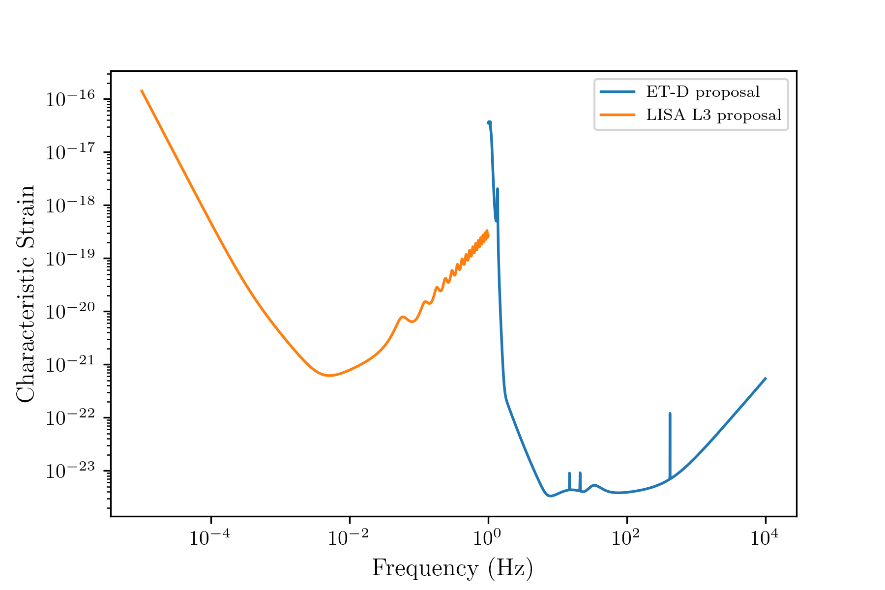
Figure 1: Proposed sensitivity curves for the Einstein Telescope [30] and LISA [29], based off existing design proposals.

2.2 Calculating detector SNR

Detector SNR $\rho_{\mathrm{det}}$ is a function of source parameters (binary mass components, spin components, redshift), source waveform models (i.e., IMRPhenomD, IMRPhenomXAS), and detector sensitivity curves. The SNR calculation is also facilitated through the use of gwent. Source and detector parameters are as described above in Section 2.1. We calculate the $M_{\mathrm{tot}}-q$ SNR grid along a range of redshifts, from $z=0.01$ up to $z=300$. Figure 2 shows SNRs for each detector as a function of binary mass ratio $q$ for fixed total masses $M_{\mathrm{tot}}=30,100,10^{3},10^{4}\,M_{\odot}$ for redshift $z=0.01$ (left panels) and $30$ (right panels). We calculate the simulated SNR for both D and XAS waveforms, represented by the solid and dotted lines respectively.

As expected, D and XAS waveforms are generally in agreement up to mass ratios $q=18$. This is much more clear in the LISA SNRs, as there is near-unnoticeable deviation between the waveforms for the case of ET at relatively lower redshifts and higher masses, as seen in the lower left panel of Figure 2. However, waveforms for ET at higher redshifts may have SNR values that differ by at least 20 orders of magnitude (as shown in the lower right panel for the case of $M_{\mathrm{tot}}=10^{3}\,M_{\odot}$). The cause of this discrepancy is unclear; the way these waveforms are simulated at these redshifts may be different. Nonetheless, we argue here that these differences are negligible in the constraint calculation later in Section 4, as these massive PBH binaries have overall negligible contribution to the event rate at high redshifts.

Given the level of agreement between the SNRs of both D and XAS waveforms across the detectors, it may be reasonable to ask “Why bother with the less efficient XAS model?” Our rationale is that at low redshifts and high sensitivities, the falloff of SNR with increasing $q$ is slow enough for us to say that even sufficiently massive high mass ratio binaries may contribute to the event rate. We can easily see this with the LISA SNR at $z=0.01$ for total binary mass $M_{\mathrm{tot}}=10^{4}\,M_{\odot}$, where the SNR only drops by one order of magnitude as mass ratio $q$ goes from $1$ to $1000$ and still well above the threshold for significant detection.

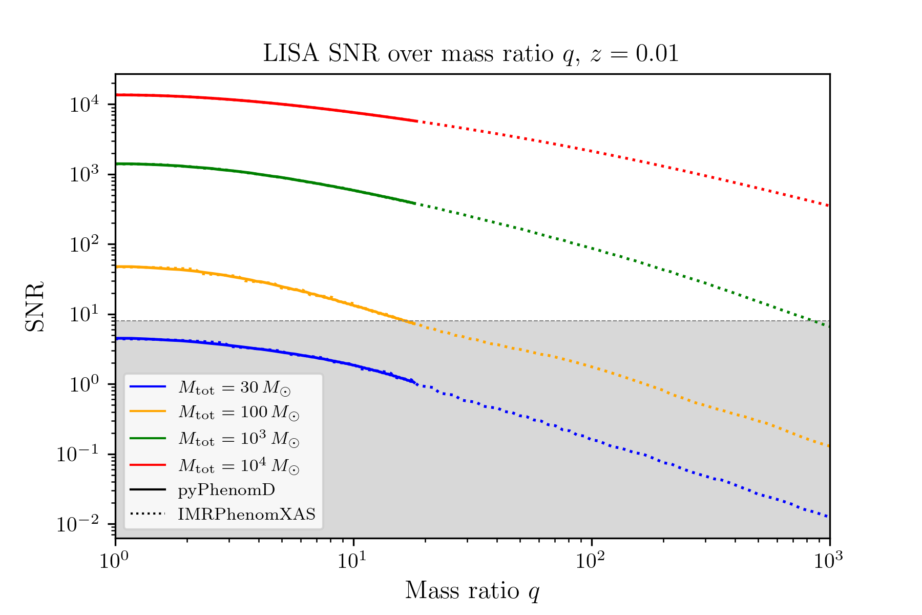
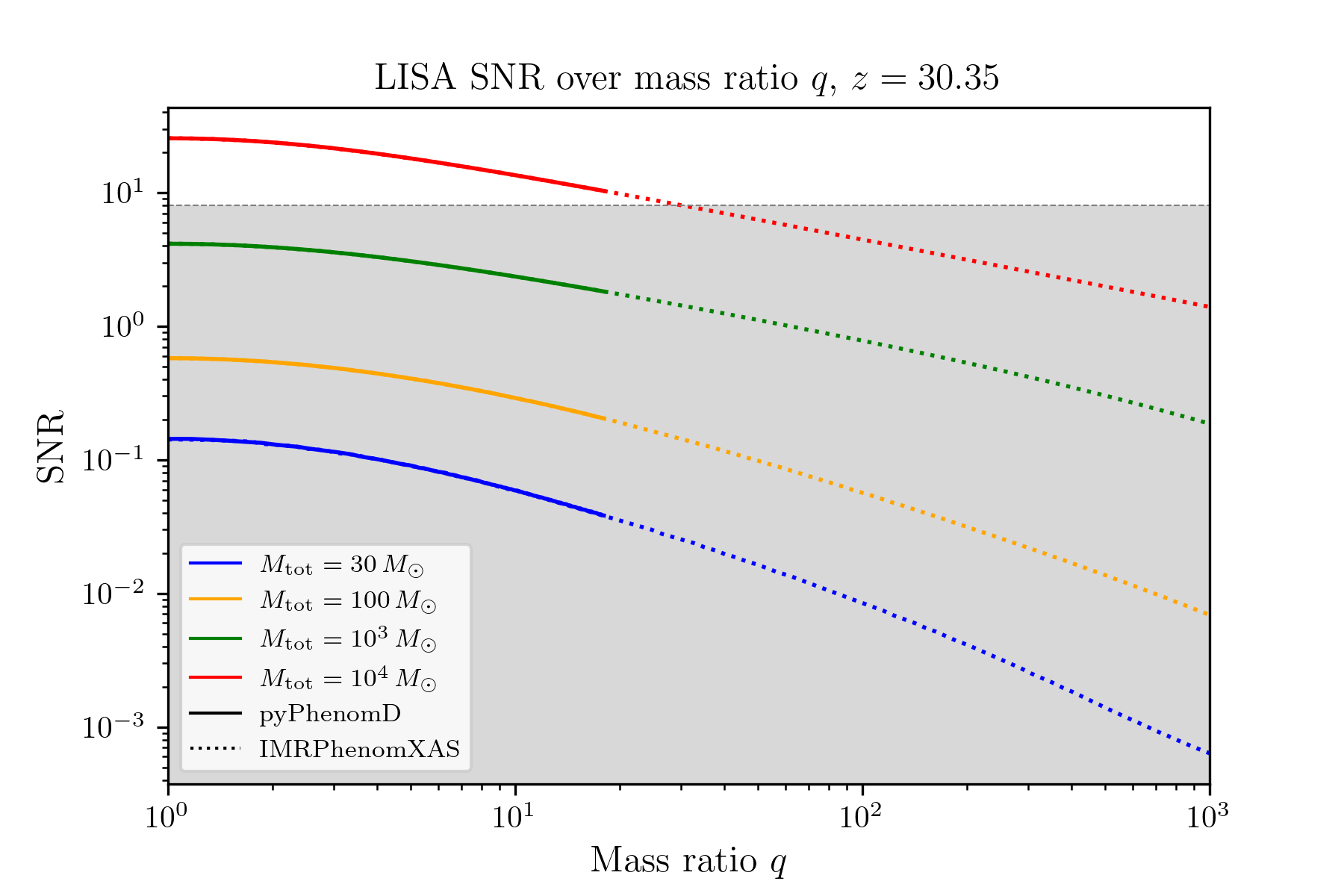
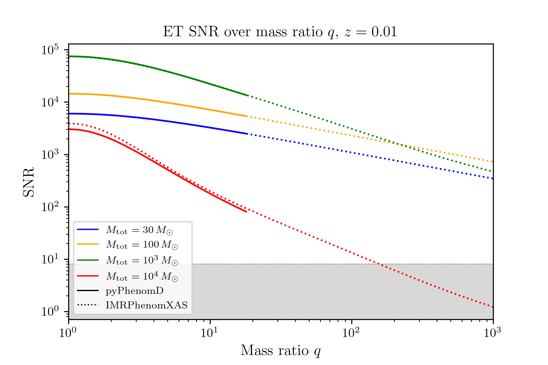
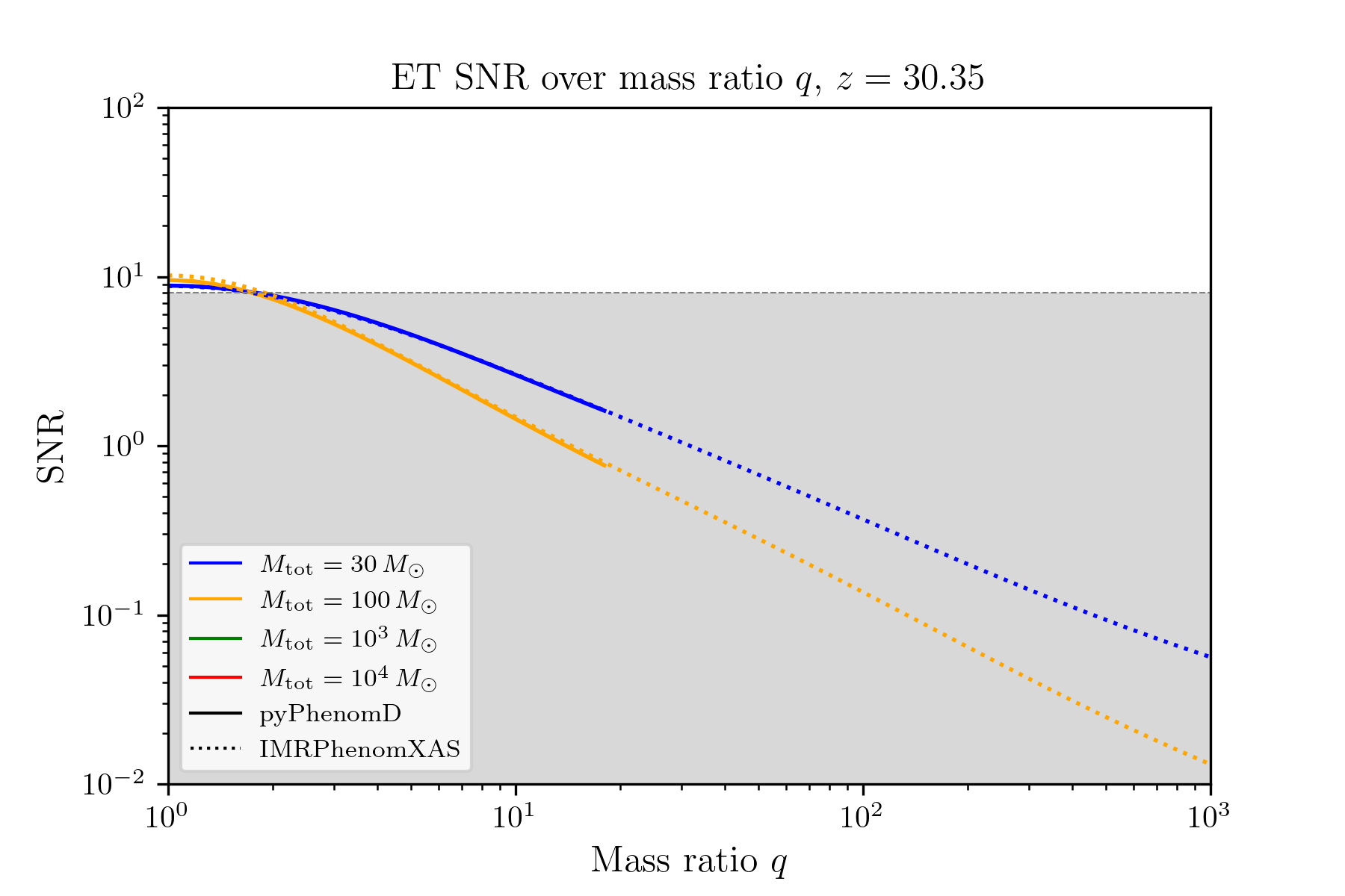
Figure 2: Detector SNRs as a function of binary mass ratio $q$ for fixed total masses $M_{\mathrm{tot}}=30,100,10^{3},10^{4}\,M_{\odot}$ for redshift $z=0.01$ (left column) and $30$ (right column). Top row shows LISA SNRs, while bottom row shows SNRs for ET. Solid curves show extent of SNR response for IMRPhenomD waveforms (up to $q=18$), while dotted curves show SNR for IMRPhenomXAS waveforms (up to $q=10^{3}$). The shaded region represents $\mathrm{SNR}\leq 8$, lower than the threshold for a significant detection.

2.3 Mass functions

In this work, we only consider the monochromatic and power law PBH mass distributions. The monochromatic mass distribution is simply defined by the Dirac delta distribution

$$\psi_{\mathrm{mono}}(M;M_{c})=\delta_{D}(M-M_{c}),$$ (2.1)

where $M_{c}$ is the central mass of the distribution. This distribution is considered primarily as a simplification, and is useful when considering symmetric mass binary GW sources.

The power law mass distribution is given by [19]:

$$\psi_{\mathrm{PL}}(M;M_{\mathrm{min}},M_{\mathrm{max}},\gamma)=\mathcal{N}_{\mathrm{PL}}M^{\gamma-1},\quad\mathcal{N}_{\mathrm{PL}}=\frac{\gamma}{M_{\mathrm{max}}^{\gamma}-M_{\mathrm{min}}^{\gamma}},$$ (2.2)

where $\mathcal{N}_{\mathrm{PL}}$ is the normalization factor for the distribution assuming $\gamma\neq 0$, and $M_{\mathrm{min}}$ and $M_{\mathrm{max}}$ are the minimum and maximum mass cut-offs of the distribution profile. The exponent $\gamma$ relates to the cosmological equation of state during the PBH formation epoch [37]. A power law mass distribution is also formulated by De Luca, et al. [38], which sets the exponent at $\gamma=-1/2$. This particular form of the mass distribution arises from assuming that collapsing primordial fluctuations form a broad and flat power spectrum in $k$-space.

For this paper, we follow the formulation set by Carr, et al. [20] in making PBH constraints from broad distributions comparable with constraints established from monochromatic distributions. Define $M_{c}$ as the reference or central mass of an arbitrary distribution. For power law distributions, we can define its bounds by

$$M*=M_{c}e^{1/\gamma},\,\mathrm{where}\,\begin{cases}M^{*}=M_{\mathrm{min}},\quad\mathrm{if}\,\gamma<0,\\ M^{*}=M_{\mathrm{max}},\quad\mathrm{if}\,\gamma>0.\end{cases}$$ (2.3)

In order to maximize the mass ratio range provided by IMRPhenomXAS, we relate the mass bounds as $M_{\mathrm{max}}=qM_{\mathrm{min}}=1000M_{\mathrm{min}}$, and set the range of $M_{c}$ the same as the range of $M_{\mathrm{tot}}$ mentioned in Sec. 2.1, i.e., $M_{c}=1-10^{4}\,M_{\odot}$ for ground-based detectors (e.g., ET), and $M_{c}=1-10^{9}\,M_{\odot}$ for space-based detectors (e.g., LISA). We also assign a spread $\sigma=1/|\gamma|$ per power law distribution, and consider values of $\sigma$ (or $|\gamma|$) as listed in Table 1. It is this shape parameter that largely determines the behaviour of the distribution and its effect on the PBH merger rate.

Shape parameter
$\sigma$	0.10	0.64	1.19	1.73	2.28	2.86	3.37	3.91	4.46	5.00
$|\gamma|$	10.0	1.55	0.84	0.58	0.44	0.35	0.30	0.26	0.22	0.20

Table 1: Shape parameters considered for our PBH power law mass distributions. Note that we consider both positive and negative values of $\gamma$.

3 Calculating the detectable merger event rate

For resolvable PBH mergers, the number of merger events per year $N_{\mathrm{det}}$ is given by [25, 39]

$$N_{\mathrm{det}}=\int\mathrm{d}z\mathrm{d}M_{1}\mathrm{d}M_{2}\,\frac{1}{1+z}\frac{\mathrm{d}V_{c}(z)}{\mathrm{d}z}\frac{\mathrm{d}^{2}R_{\mathrm{PBH}}}{\mathrm{d}M_{1}\mathrm{d}M_{2}}p_{\mathrm{det}}(M_{1},M_{2},z).$$ (3.1)

Here, $V_{c}(z)$ is the comoving volume per unit redshift, and $p_{\mathrm{det}}$ is the binary detectability of any mass pair $M_{1}$ and $M_{2}$ at a redshift $z$ for some particular GW detector, and $R_{\mathrm{PBH}}$ is the differential PBH merger rate. $p_{\mathrm{det}}$ is determined by the ratio between the optimal detector signal-to-noise ratio (SNR) $\rho_{\mathrm{det}}$ and a preset detection threshold $\rho_{\mathrm{thr}}$, which we set to be equal to 8. We use the form of $p_{\mathrm{det}}$ as described in the Appendix of [39] for a single detector.

The differential PBH merger rate $R_{\mathrm{PBH}}$ is given by [25, 40]

$$\frac{\mathrm{d}^{2}R_{\mathrm{PBH}}}{\mathrm{d}M_{1}\mathrm{d}M_{2}} =\frac{1.6\times 10^{6}}{\mathrm{Gpc}^{3}\,\mathrm{yr}}f^{53/37}_{\mathrm{PBH}}\left(\frac{M_{\mathrm{tot}}^{2}}{M_{1}M_{2}}\right)^{34/37}\left(\frac{t}{t_{0}}\right)^{-34/37}\left(\frac{M_{\mathrm{tot}}}{M_{\odot}}\right)^{-32/37}\times$$

$$\times S(M_{1},M_{2},f_{\mathrm{PBH}},t)\psi(M_{1})\psi(M_{2}),$$ (3.2)

where $M_{1}$ and $M_{2}$ are the principal masses of the PBH binary, $M_{\mathrm{tot}}=M_{1}+M_{2}$ is the initial total mass of the binary upon formation, and the suppression factor $S$ accounts for disruption due to inhomogeneities in the DM fluid and neighboring PBHs, as well as disruption due to substructures forming later in the Universe [40, 23]. $\psi(M)$ denotes the PBH mass distribution upon formation. We will only consider monochromatic and power law mass functions upon PBH formation, given by Equations (2.1) and (2.2). We will also assume that these distributions are relatively static throughout the evolution of the binaries, and ignore any possible accretion and initial clustering effects.

Note that the calculation of the event rate $N_{\mathrm{det}}$ involves both an integration (averaging) across not just a redshift range but also across a mass range. For monochromatic PBH mass distributions, this mass range collapses to $M_{c}$; all detectable PBH merger events associated with the reference mass $M_{c}$ are due to binaries of total mass with the same order of magnitude as the reference mass $(M_{\mathrm{tot}}=2M_{c})$. However, this is not the case for broad mass distributions such as power law. Instead, each event rate attributed to a power law distribution $\psi$ with parameters $M_{c}$ and $\gamma$ contains the averaged contribution of all binaries with component masses within the range of $M_{\mathrm{min}}$ to $M_{\mathrm{max}}$ sampled from $\psi$. Note that because of how the mass range bounds are defined in Sec. 2.3 and Eq. (2.3), the resulting integration bounds in Eq. (3.1) include masses outside the detection ranges we have set in for LISA and ET in Sec. 2.2.

4 Constraints on PBH abundance

Before we continue to the constraint calculation, let us first summarize the assumptions we set in the previous sections:

• PBH source binary total mass $M_{\mathrm{tot}}$ detection range: $1-10^{4}\,M_{\odot}$ for ET, $1-10^{9}\,M_{\odot}$ for LISA.

• PBH source binary mass ratios: $q=1-1000$.

• PBH source binary component spins: $\chi_{1}=\chi_{2}=0$.

• Source waveform model: IMRPhenomXAS.

• Detector SNR threshold: $\rho_{\mathrm{thr}}=8$.

• Simulated observation time: 1 year.

In addition, assumptions on the mass distribution and merger rate calculations are as follows:

• Mass functions: monochromatic and power law.

• Power law reference mass $M_{c}$ range: $1-10^{4}\,M_{\odot}$ for ET, $1-10^{9}\,M_{\odot}$ for LISA.

• Power law exponent $\gamma$ range: $|\gamma|\in[0.2,10]$ for both $\gamma<0$ and $\gamma>0$.

• Power law cutoffs determined by reference mass $M_{c}$ and maximum $q=1000$,

• Initial clustering and accretion effects on the PBH merger rate are ignored.

With the setup laid out, we now outline the method for calculating the $f_{\mathrm{PBH}}$ constraints for power law PBH distributions. We first define a log-spaced grid in $M_{\mathrm{tot}}$ and a linearly-spaced grid in $q$ and pre-calculate the SNR tables for each detector using gwent [28]; the ranges in $q$ and $M_{\mathrm{tot}}$ (per detector) are as specified above. This results in a $50\times 50$ $M_{\mathrm{tot}}-q$ SNR table per redshift, for 100 equal log-spaced bins from $z=0$ to $300$. We do this for both LISA and ET, preparing a total of 100 SNR tables each.

We use these SNR values $\rho_{\mathrm{det}}$ to obtain $p_{\mathrm{det}}$ in Eq. (3.1) for a given combination of $M_{1}$, $M_{2}$, and $z$. The bounds of mass integration are determined by $M_{\mathrm{min}}$ and $M_{\mathrm{max}}$. The bounds for redshift integration set to be $z\in[0.01,30]$ for low redshift events, and $z\in[30,300]$ for high redshift events.

Next, we obtain the PBH integrated event rate $N_{\mathrm{det}}$ for each $(M_{c},\gamma,f_{\mathrm{PBH}})$ point in the parameter space, where we choose 100 equal log-spaced bins in $M_{c}$ for the range specified above (per detector) and $f_{\mathrm{PBH}}$ runs from $10^{-8}$ to $1$ in 100 equal log-spaced bins. Recall that there are 20 values of $\gamma$ considered, 10 with positive and 10 with negative signs, for values of $|\gamma|$ listed in Table 1. Note that $f_{\mathrm{PBH}}$ and $\gamma$ enter through the differential PBH merger rate given in Eq. (3.2).

Once all event rates within the parameter space have been calculated, we scan through the $f_{\mathrm{PBH}}$ range for each $(M_{c},\gamma)$ pair and pick the minimum $f_{\mathrm{{PBH}}}$ value where the event rate $N_{\mathrm{det}}\geq 1$. These minimum $f_{\mathrm{PBH}}$ values serve as our constraint for a particular reference mass and power law profile.

Figure 3: Minimum PBH abundance $f_{\mathrm{PBH}}$ constraint curves for LISA (top panels) and ET (bottom panels), integrated in redshift from $z\in[0.01,30]$. Dashed lines indicate constraints set by power law distributions with exponent $\gamma<0$ (left panels) and $\gamma>0$ (right panels). Solid gray region is based off the monochromatic constraints obtained in [25] using D waveforms, while the dotted purple line is the monochromatic constraint we have obtained using XAS waveforms.

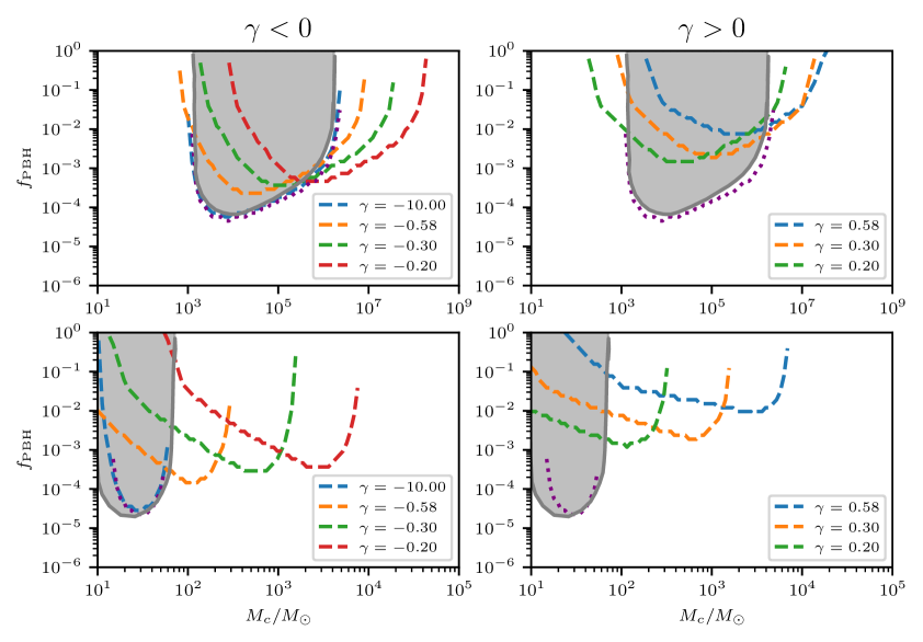
Figure 4: Minimum PBH abundance $f_{\mathrm{PBH}}$ constraint curves for LISA (top panels) and ET (bottom panels), integrated in redshift from $z\in[30,300]$. Dashed lines indicate constraints set by power law distributions with exponent $\gamma<0$ (left panels) and $\gamma>0$ (right panels). Solid gray region is based off the monochromatic constraints obtained in [25] using D waveforms, while the dotted purple line is the monochromatic constraint we have obtained using XAS waveforms.

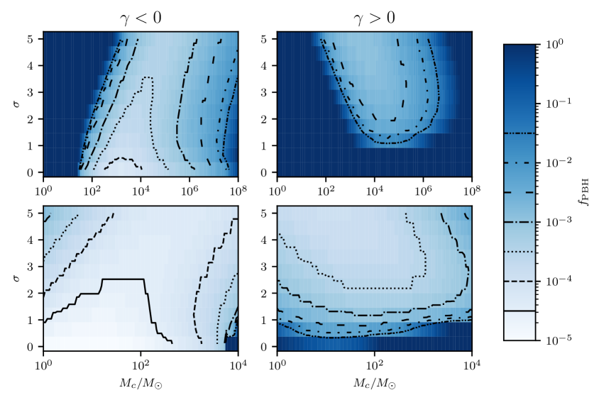
Figure 5: $M_{c}-\sigma$ contour plots for LISA (top panels) and ET (bottom panels), integrated in redshift from $z\in[0.01,30]$. Values of the $f_{\mathrm{PBH}}$ contours are indicated by the legend on the color bars. Dark blue regions are classified as unconstrained by the detector model.

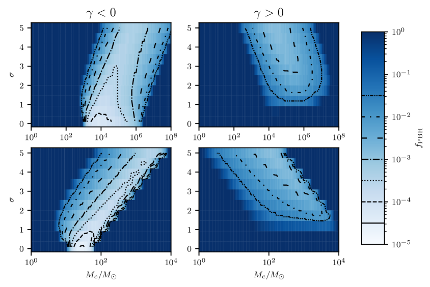
Figure 6: $M_{c}-\sigma$ contour plots for LISA (top panels) and ET (bottom panels), integrated in redshift from $z\in[30,300]$. Values of the $f_{\mathrm{PBH}}$ contours are indicated by the legend on the color bars. Dark blue regions are classified as unconstrained by the detector model.

Figures 3 & 4 show the $f_{\mathrm{PBH}}$ constraint curves as a function of reference mass $M_{c}$ for low and high redshifts, respectively. In both Figures, the panels show projected constraints for LISA (top panels) and ET (bottom panels), and for power law distributions with exponent $\gamma<0$ (left panels) and $\gamma>0$ (right panels). The dashed lines indicate constraints generated from the power law distributions, while the dotted line is the XAS constraint for monochromatic distributions. The solid gray regions are the monochromatic constraints calculated by De Luca, et al. [25] using D waveforms.

Figures 5 & 6 show how $f_{\mathrm{PBH}}$ changes with $\sigma=1/|\gamma|$. White and light blue regions represent power law distribution parameters where there is an appreciably low minimum abundance constraint (i.e., $f_{\mathrm{PBH}}\lesssim 10^{-2}$), while the parameter space in the dark blue regions would require at least percent-level abundance to obtain a resolvable signal in one observation year. We classify regions which require $f_{\mathrm{PBH}}\geq 1$ as unconstrained, i.e., the detector model cannot set a physical constraint for a mass distribution model within that region of parameter space. These are shown with the darkest blue color (corresponding to $f_{\mathrm{PBH}}=1$ in the color scale).

One readily apparent feature seen in Figures 3 & 4 is that higher abundances are generally required for the power law distributions, relative to the monochromatic cases, in order to obtain an event detection rate of at least unity. For $\gamma>0$ (right panels of both Figures), higher exponents raise the minimum abundances. We can see the largest difference for $\gamma=0.58$, necessitating $f_{\mathrm{PBH}}$ abundances up two orders of magnitude greater than the monochromatic case for low redshift, and up to three orders of magnitude at high redshift. For higher exponents (corresponding to $\sigma\lesssim 1$), the derived required minimum abundances exceed 1, which is unphysical and implies that this regime is unconstrained — as we can see in the dark blue regions of the right panels in Figures 5 & 6.

On the other hand, for $\gamma<0$, decreasing the exponent (i.e., increasing the magnitude of $|\gamma|$) makes the curve approach that of the monochromatic XAS case, as seen in the left panels of Figures 3 & 4. This can be seen in the case of $\gamma=-10$, which has a minimum abundance curve almost coincident with the monochromatic case. Note however that there may be instances where a power law distribution would have slightly lower minimum abundances over specific mass ranges. Specifically, we find that this is the case for the ET constraints at low redshifts, over the interval of $10^{3}\,M_{\odot}<M_{c}<10^{4}\,M_{\odot}$, as seen in the bottom left panel of Figure 3. At higher redshifts, the general trend of higher minimums is preserved throughout the mass range, as seen in the bottom left panel of Figure 4.

Another consequence of assuming a broad power law mass distribution is how the constraint window set by the reference masses shift as we change the shape parameter $\gamma$. In the case of LISA (top panels of Figures 3 & 4), the constraint window moves to the right relative to the monochromatic curve as we increase $\gamma$. For ET at low redshifts (bottom panels of Figure 3), the constraint curve tilts in favor of lower relative minimums at higher reference masses; for positive exponents, this trend can be described more as a flattening of the curve overall. This apparent tilting is not present for ET constraints at higher redshift (bottom panels of Figure 4), which instead show a shifting constraint window similar to the LISA constraints.

Comparing across redshift ranges in Figures 3 to 6 present to us a clear difference in the width of the constraint windows between low and high redshifts. This is a natural consequence of the narrowing detection window at higher redshifts, although it is worth discussing how the high redshift constraint window changes as we increase $\gamma$. Unlike the low redshift cases which generally fall within the area of the monochromatic windows, the constraint windows for power law distributions at high redshift can significantly deviate from their respective monochromatic windows. At higher exponents, the trends relative to monochromatic tend to wider mass windows (up to two decades in $M_{c}$), higher minimum abundances (as much as three orders of magnitude in $f_{\mathrm{PBH}}$), and an overall shift to constraining higher reference masses.

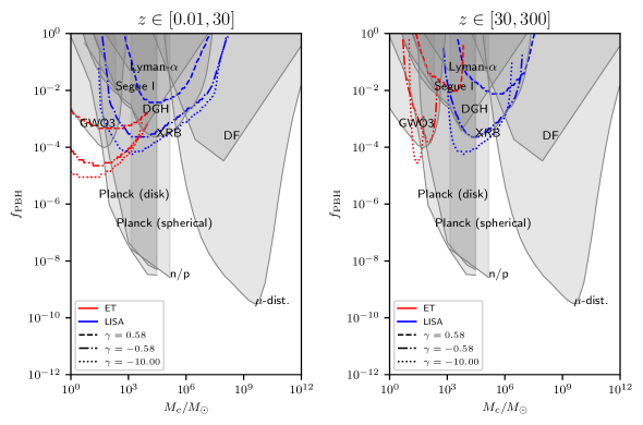
Figure 7: Projected ET and LISA constraints for PBH power law mass distributions with exponents $\gamma=(-10,\,-0.58,\,0.58)$, compared against existing present-day monochromatic constraints (solid lines, colored in grey). Left and right panels correspond to low and high observation redshifts, respectively. Constraints considered in this figure include constraints from gravitational wave observations in the LVK O3 run (GWO3) [24], Planck CMB measurements [15], dwarf galaxy dynamics (Segue I) [41] and heating (DGH) [42, 43], Lyman-$\alpha$ observations [18], X-ray binary observations (XRB) [44], dynamical friction (DF) [17], the neutron-to-proton ratio (n/p) [45], and CMB $\mu$-distortion [46]. Note that for the $\mu$-distortion constraint, we chose the FIRAS value corresponding to large non-Gaussianity $(p=0.5)$.

Figure 7 summarizes our results in the context of existing monochromatic constraints from the literature. Here, we chose to show our ET and LISA constraints for the most positive and most negative values of $\gamma$ that still provided constraints ($\gamma=-10.00$ and $0.58$, respectively), as well as for $\gamma=-0.58$, which most closely corresponds to the power law mass distribution formulated by De Luca, et al. [38], for comparison. We compare these against constraints from gravitational-wave observations in the LIGO-Virgo-KAGRA (LVK) O3 run (GWO3) [24], Planck CMB measurements (assuming spherical and disk accretion) [15], dwarf galaxy dynamics (Segue I) [41] and heating (DGH) [42, 43], Lyman-$\alpha$ observations [18], X-ray binary observations (XRB) [44], dynamical friction (DF) [17], the neutron-to-proton ratio (n/p) [45], and CMB $\mu$-distortion [46], shown as the grey regions on the plots. We show the same regions on both low and high redshift plots for the sake of easy comparison, although we acknowledge that some of these constraints may be relaxed at high redshift. We note that each of these existing constraints have varying degrees of uncertainty and assumptions. In addition, these constraints are expected to change depending on the shape of the mass distribution considered [20].

As previously reported by De Luca, et al. [25], future GW observatories open a window to detect high-redshift PBHs, as illustrated in the right panel of Figure 7. LISA and ET observations would complement each other by probing different mass windows. This is true regardless of power law shape, albeit the constraints become less stringent for increasingly positive power law exponents.

At low redshift, ET projections potentially lower the upper bound of abundance set by LVK GWO3, at least for negative power law exponents. On the other hand, low-redshift LISA projections overlap with existing constraints from local observations, particularly those coming from present-day constraints on PBH accretion (DGH, XRB) [42, 43, 44] and dynamical effects on dwarf galaxies (Segue I) [41]. These local constraints may potentially be relaxed at high redshift, or notably even disappear in the case of the LVK GWO3 constraints. However, going to high redshift does not let us evade constraints set by CMB $\mu$-distortion [15, 46] and BBN observations (“n/p”) [45], which most strongly constrain the region with $M_{c}$ above $10^{2}\,M_{\odot}$. We remark that even with a choice of a particularly conservative form of the $\mu$-distortion constraints (with non-Gaussianity parameter $p=0.5$), there is little to no room for PBHs of mass $\sim 10^{6}\,M_{\odot}$ at abundances $f\sim 10^{-4}$.

We note that Ref. [20] reports how the monochromatic constraints from the Segue I and Planck CMB constraints shift for extended mass distributions, although these results are not shown here to avoid overcrowding the figures. Our contribution to the literature is to show how the monochromatic high-redshift constraints from GW observations (as reported in e.g., Ref. [25]) are expected to shift for extended mass distributions.

5 Conclusions and outlook

In this paper, we set projected $f_{\mathrm{PBH}}$ abundance constraints from simulated LISA and ET observations for extended PBH mass distributions. We achieved this by considering broad power law distributions for a range of negative and positive exponents $\gamma$, and considering binary mergers with mass ratios up to $q=1000$, and modeling these resolvable mergers using IMRPhenomXAS waveforms. We observe two primary trends in our results, regardless of redshift. For positive exponents, increasing $\gamma$ results in much less stringent constraints shifted towards higher PBH masses. For negative exponents, the constraints rapidly converge to the respective monochromatic cases when $\gamma\lesssim-1$. We remark that the latter trend is actually present for non-GW constraints reported in Ref. [20] for $\gamma<0$, although to our knowledge we are the first to explicitly show this convergence for GW-derived constraints. It is also interesting to note that Ref. [38] points out that negative-tilted broad primordial perturbation spectra will lead to mass functions close to that of the monochromatic case. Establishing a systematic relation between broad perturbation spectra and their resulting mass functions will be a next step in refining PBH population models and its effects on the merger rate.

We find that, under our current setup and assumptions, broadly extending the mass distribution generally does not enable us to evade existing constraints for the mass ranges we have considered. If the ET and LISA constraint curves in Figure 7 are upper bounds on abundance from non-detection, then only ET constraints at low redshift for $\gamma<0$ would give us any significant new information. ET bounds for $\gamma>0$, as well as LISA bounds for all $\gamma$ are all subsumed by the monochromatic LVK GWO3, CMB Planck, and $\mu$-distortion constraints (noting that the latter two also apply at high redshifts). Even if these monochromatic constraints are modified accordingly to apply to extended mass distributions, the aforementioned projected bounds are expected to remain within these constraints.

Keeping assumptions about our PBH models constant, one way to evade the existing constraints is to have a detector that could probe at either higher sensitivities (reducing $f_{\mathrm{PBH}}$ necessary for a detection) or at higher mass ranges ($M\gtrsim 10^{11}\,M_{\odot}$) across a wide range of redshifts. Setting aside the feasibility of such a detector, however, evading the $\mu$-distortion bound by simultaneously lowering the required abundance and raising the PBH mass would quickly run us into the incredulity limit, which sets the abundance lower bound for $M\sim 10^{11}\,M_{\odot}$ at $f_{\mathrm{PBH}}\sim 10^{-10}$ [17].

There are other, less detector-dependent approaches to evading the existing constraints. The first is to consider subsolar ($M<1\,M_{\odot}$) mergers, as well as potential constraints derived from the stochastic GW background. Both are beyond the scope of this current study, although they are worth investigating in the context of extended PBH mass distributions. Modifying the model to account for phenomenological uncertainties such as clustering [25, 47, 48] and accretion [49, 50] may also provide an avenue for evasion. Incorporating broadly extended mass distributions to these model additions may however introduce new uncertainties, such as the implications of an extended distribution to the initial clustering, as well as potential changes to the local PBH accretion environments as a result of strong initial clustering.

Finally, we remark that broadly extended mass distributions may be relevant when considering the PBH merger rate of initially three-body configurations [51, 52]. This merger rate is considered subdominant to the the two-body merger rate in the regime considered by LVK [24], but their analysis is restricted to narrow $(\sigma\lesssim 1.2)$ mass distributions. For these investigations, it would be interesting to consider even flatter distributions with $|\gamma|\sim 0$. Generally, more work is needed in order to establish the nuance of how these very broad mass distributions affect the overall PBH merger rate.

References

- [1] LIGO Scientific Collaboration and Virgo Collaboration collaboration, GWTC-2: Compact Binary Coalescences Observed by LIGO and Virgo during the First Half of the Third Observing Run, Phys. Rev. X 11 (2021) 021053.
- [2] Z.C. Zhao and S. Wang, Bayesian implications for the primordial black holes from NANOGrav’s pulsar-timing data using the scalar-induced gravitational waves, Universe 9 (2023) .
- [3] A. Afzal, G. Agazie, A. Anumarlapudi, A.M. Archibald, Z. Arzoumanian, P.T. Baker et al., The NANOGrav 15 yr data set: Search for signals from new physics, Astrophys. J. Lett. 951 (2023) L11.
- [4] B. Carr, K. Kohri, Y. Sendouda and J. Yokoyama, Constraints on primordial black holes, Rep. Prog. Phys. 84 (2021) 116902.
- [5] P. Villanueva-Domingo, O. Mena and S. Palomares-Ruiz, A brief review on primordial black holes as dark matter, Front. Astron. Space Sci. 8 (2021) 681084.
- [6] H. Niikura, M. Takada, S. Yokoyama, T. Sumi and S. Masaki, Constraints on earth-mass primordial black holes from OGLE 5-year microlensing events, Phys. Rev. D 99 (2019) 083503.
- [7] N. Smyth, S. Profumo, S. English, T. Jeltema, K. McKinnon and P. Guhathakurta, Updated constraints on asteroid-mass primordial black holes as dark matter, Phys. Rev. D 101 (2020) 063005.
- [8] K. Griest, A.M. Cieplak and M.J. Lehner, New limits on primordial black hole dark matter from an analysis of Kepler source microlensing data, Phys. Rev. Lett. 111 (2013) 181302.
- [9] K. Griest, A.M. Cieplak and M.J. Lehner, Experimental limits on primordial black hole dark matter from the first 2 yr of Kepler data, Astrophys. J. 786 (2014) 158.
- [10] C. Alcock, R.A. Allsman, D.R. Alves, T.S. Axelrod, A.C. Becker, D.P. Bennett et al., MACHO project limits on black hole dark matter in the range, Astrophys. J. 550 (2001) L169.
- [11] M. Zumalacárregui and U. Seljak, Limits on stellar-mass compact objects as dark matter from gravitational lensing of Type Ia supernovae, Phys. Rev. Lett. 121 (2018) 141101.
- [12] A. Barnacka, J.-F. Glicenstein and R. Moderski, New constraints on primordial black holes abundance from femtolensing of gamma-ray bursts, Phys. Rev. D 86 (2012) 043001.
- [13] Tisserand, P., Le Guillou, L., Afonso, C., Albert, J. N., Andersen, J., Ansari, R. et al., Limits on the Macho content of the galactic halo from the EROS-2 survey of the magellanic clouds, A&A 469 (2007) 387.
- [14] A.M. Green, Microlensing and dynamical constraints on primordial black hole dark matter with an extended mass function, Phys. Rev. D 94 (2016) 063530.
- [15] P.D. Serpico, V. Poulin, D. Inman and K. Kohri, Cosmic microwave background bounds on primordial black holes including dark matter halo accretion, Phys. Rev. Res. 2 (2020) 023204.
- [16] B.J. Carr and M. Sakellariadou, Dynamical constraints on dark matter in compact objects, Astrophys. J. 516 (1999) 195.
- [17] B. Carr and J. Silk, Primordial black holes as generators of cosmic structures, MNRAS 478 (2018) 3756 [https://academic.oup.com/mnras/article-pdf/478/3/3756/25077116/sty1204.pdf].
- [18] R. Murgia, G. Scelfo, M. Viel and A. Raccanelli, Lyman- forest constraints on primordial black holes as dark matter, Phys. Rev. Lett. 123 (2019) 071102.
- [19] N. Bellomo, J.L. Bernal, A. Raccanelli and L. Verde, Primordial black holes as dark matter: converting constraints from monochromatic to extended mass distributions, J. Cosmol. Astropart. Phys. 2018 (2018) 004.
- [20] B. Carr, M. Raidal, T. Tenkanen, V. Vaskonen and H. Veermäe, Primordial black hole constraints for extended mass functions, Phys. Rev. D 96 (2017) 023514.
- [21] K.W.K. Wong, G. Franciolini, V. De Luca, V. Baibhav, E. Berti, P. Pani et al., Constraining the primordial black hole scenario with bayesian inference and machine learning: The GWTC-2 gravitational wave catalog, Phys. Rev. D 103 (2021) 023026.
- [22] M. Raidal, V. Vaskonen and H. Veermäe, Gravitational waves from primordial black hole mergers, J. Cosmol. Astropart. Phys. 2017 (2017) 037.
- [23] G. Hütsi, M. Raidal, V. Vaskonen and H. Veermäe, Two populations of LIGO-Virgo black holes, J. Cosmol. Astropart. Phys. 2021 (2021) 068.
- [24] M. Andrés-Carcasona, A.J. Iovino, V. Vaskonen, H. Veermäe, M. Martínez, O. Pujolàs et al., Constraints on primordial black holes from LIGO-Virgo-KAGRA O3 events, 2024.
- [25] V.D. Luca, G. Franciolini, P. Pani and A. Riotto, The minimum testable abundance of primordial black holes at future gravitational-wave detectors, J. Cosmol. Astropart. Phys. 2021 (2021) 039.
- [26] K.K.Y. Ng, G. Franciolini, E. Berti, P. Pani, A. Riotto and S. Vitale, Constraining high-redshift stellar-mass primordial black holes with next-generation ground-based gravitational-wave detectors, Astrophys. J. Lett. 933 (2022) L41.
- [27] G.L.A. Dizon and R. Reyes, Role of extended mass distributions in minimum testable primordial black hole abundances from high-redshift mergers, in Proceedings of the Samahang Pisika ng Pilipinas, vol. 40, (Legazpi, Philippines), pp. SPP–2022–1B–03, 2022.
- [28] A.R. Kaiser and S.T. McWilliams, Sensitivity of present and future detectors across the black-hole binary gravitational wave spectrum, Class. Quantum Gravity 38 (2021) 055009.
- [29] P. Amaro-Seoane, H. Audley, S. Babak, J. Baker, E. Barausse, P. Bender et al., Laser Interferometer Space Antenna, 2017. https://doi.org/10.48550/arXiv.1702.00786.
- [30] S. Hild, M. Abernathy, F. Acernese, P. Amaro-Seoane, N. Andersson, K. Arun et al., Sensitivity studies for third-generation gravitational wave observatories, Class. Quant. Grav. 28 (2011) 094013.
- [31] T. Harada, C.-M. Yoo, K. Kohri and K.-I. Nakao, Spins of primordial black holes formed in the matter-dominated phase of the universe, Phys. Rev. D 96 (2017) 083517.
- [32] T. Chiba and S. Yokoyama, Spin distribution of primordial black holes, Prog. Theor. Phys. 2017 (2017) 083E01 [https://academic.oup.com/ptep/article-pdf/2017/8/083E01/19488901/ptx087.pdf].
- [33] S. Husa, S. Khan, M. Hannam, M. Pürrer, F. Ohme, X.J. Forteza et al., Frequency-domain gravitational waves from nonprecessing black-hole binaries. I. New numerical waveforms and anatomy of the signal, Phys. Rev. D 93 (2016) 044006.
- [34] S. Khan, S. Husa, M. Hannam, F. Ohme, M. Pürrer, X.J. Forteza et al., Frequency-domain gravitational waves from nonprecessing black-hole binaries. II. A phenomenological model for the advanced detector era, Phys. Rev. D 93 (2016) 044007.
- [35] M.C. Digman and N.J. Cornish, Parameter estimation for stellar-origin black hole mergers in lisa, Phys. Rev. D 108 (2023) 023022.
- [36] G. Pratten, S. Husa, C. García-Quirós, M. Colleoni, A. Ramos-Buades, H. Estellés et al., Setting the cornerstone for a family of models for gravitational waves from compact binaries: The dominant harmonic for nonprecessing quasicircular black holes, Phys. Rev. D 102 (2020) 064001.
- [37] B.J. Carr, The primordial black hole mass spectrum, Astrophys. J. 201 (1975) 1.
- [38] V. De Luca, G. Franciolini and A. Riotto, On the primordial black hole mass function for broad spectra, Phys. Lett. B 807 (2020) 135550.
- [39] M. Dominik, E. Berti, R. O’Shaughnessy, I. Mandel, K. Belczynski, C. Fryer et al., Double compact objects. III. Gravitational-wave detection rates, Astrophys. J. 806 (2015) 263.
- [40] M. Raidal, C. Spethmann, V. Vaskonen and H. Veermäe, Formation and evolution of primordial black hole binaries in the early universe, J. Cosmol. Astropart. Phys. 2019 (2019) 018.
- [41] S.M. Koushiappas and A. Loeb, Dynamics of dwarf galaxies disfavor stellar-mass black holes as dark matter, Phys. Rev. Lett. 119 (2017) 041102.
- [42] P. Lu, V. Takhistov, G.B. Gelmini, K. Hayashi, Y. Inoue and A. Kusenko, Constraining primordial black holes with dwarf galaxy heating, Astrophys. J. Lett. 908 (2021) L23.
- [43] V. Takhistov, P. Lu, G.B. Gelmini, K. Hayashi, Y. Inoue and A. Kusenko, Interstellar gas heating by primordial black holes, J. Cosmol. Astropart. Phys. 2022 (2022) 017.
- [44] Y. Inoue and A. Kusenko, New x-ray bound on density of primordial black holes, J. Cosmol. Astropart. Phys. 2017 (2017) 034.
- [45] K. Inomata, M. Kawasaki and Y. Tada, Revisiting constraints on small scale perturbations from big-bang nucleosynthesis, Phys. Rev. D 94 (2016) 043527.
- [46] T. Nakama, B. Carr and J. Silk, Limits on primordial black holes from distortions in cosmic microwave background, Phys. Rev. D 97 (2018) 043525.
- [47] S. Young and C.T. Byrnes, Initial clustering and the primordial black hole merger rate, J. Cosmol. Astropart. Phys. 2020 (2020) 004.
- [48] G. Ballesteros, P.D. Serpico and M. Taoso, On the merger rate of primordial black holes: effects of nearest neighbours distribution and clustering, J. Cosmol. Astropart. Phys. 2018 (2018) 043.
- [49] G. Hütsi, M. Raidal and H. Veermäe, Small-scale structure of primordial black hole dark matter and its implications for accretion, Phys. Rev. D 100 (2019) 083016.
- [50] V. De Luca, G. Franciolini, P. Pani and A. Riotto, Constraints on primordial black holes: The importance of accretion, Phys. Rev. D 102 (2020) 043505.
- [51] V. Vaskonen and H. Veermäe, Lower bound on the primordial black hole merger rate, Phys. Rev. D 101 (2020) 043015.
- [52] M. Raidal, V. Vaskonen and H. Veermäe, Formation of primordial black hole binaries and their merger rates, 2024.