Persuasion and Optimal Stopping

Abstract

We provide a unified analysis of how dynamic information should be designed in optimal stopping problems: a principal controls the flow of information about a payoff relevant state to persuade an agent to stop at the right time, in the right state, and choose the right action. We further show that for arbitrary preferences, intertemporal commitment is unnecessary: optimal dynamic information designs can always be made revision-proof.

1  Introduction

At the heart of many economic decisions lies an optional stopping problem paired with a choice problem—a decision maker chooses when to stop gathering information and what irrevocable action to take. The decision maker’s stopping time and action are, in turn, jointly determined by the flow of information over time, which makes information a powerful tool for shaping both timing and choice. For example, a company may strategically reveal information about its financial health to guide investors in selling their shares at the right time in different states. An employer may strategically reveal information about the quality of a project to guide employees to exert the right amount of effort in different states. An advisor may strategically release information about her advisee’s true talent to guide him to graduate at the right time and choose the right career path.

In each of these examples, there is a common tension between persuasion and timing: on the one hand, the information that—from the principal’s point of view—best shapes the agent’s actions is typically quite specific, and falls short of complete information; on the other hand, to manipulate the timing of the action, the sender must release enough future information as a carrot to incentivize waiting. We develop tools for solving the principal’s problem and use them to deliver insights on the value and form of optimal dynamic persuasion.

Example: Alibi or Fingerprint?

To illustrate our model, consider the example of a prosecutor (principal) trying to persuade a jury (agent) as in the leading example of Kamenica and Gentzkow (2011). The defendant is either guilty or innocent. The jury decides whether to convict or acquit the defendant and gets utility 1 from choosing the just action and 0 otherwise. The prosecutor receives utility 1 from conviction and 0 from acquittal. The common prior in the defendant’s guilt is still within reasonable doubt; that is, sans further information, the jurors would choose to acquit the defendant.

Unique to our model, the trial proceeds over time: the jury is impatient, and waiting is costly. The prosecutor values both conviction and delay, and these might be complements (perhaps because this saves her the cost of switching cases, or because she values publicity conditional on winning) or substitutes (perhaps because she gets paid if the defendant is convicted, or if the trial drags on for long enough, but not extra if both occur). The prosecutor chooses the process of investigation, formalized as a history and state-dependent sequence of distributions of signal realizations. Concretely, the set of feasible investigation technologies is fully flexible and includes—but is not limited to—two canonical investigation tactics:

• Alibi: the prosecutor investigates the potential alibis i.e., searches for decisive evidence of innocence. This tactic leads to a random arrival of evidence that proves innocence, and the absence of the evidence leads to the belief of guilt drifting up.

• Fingerprint: the prosecutor searches for decisive forensic evidence like the defendant’s fingerprint or DNA at the crime scene. This tactic leads to a random arrival of decisive evidence that proves guilt, and the absence of the evidence leads to the belief of guilt drifting down.

Before introducing the optimal investigation tactics, it will be helpful to consider the static persuasion benchmark of Kamenica and Gentzkow (2011), which leads to either a firm belief of innocence or a belief of guilt that is “just enough for conviction”. This is often suboptimal when the investigator values delay: since the jury gets no additional utility from such information, there is no way to induce the impatient jury to wait any longer while maintaining the same decision beliefs: the investigator would rather release a little more information as a carrot to induce the jury to wait. Thus, in our dynamic environment, the prosecutor must now trade off persuasion against delay. We will subsequently solve for the optimal investigation strategy when the signal structure can be flexibly chosen. Three conditions on the primitives determine the optimal strategy:

1. Time risk attitudes: when the prosecutor is relatively time-risk-averse, the optimal strategy is to search for either alibi or fingerprint and release information immediately.

2. Complementarity between persuasion and delay: Whether Alibi or Fingerprint is optimal depends on the degree to which the prosecutor would like to positively or negatively correlate stopping times with her preferred action. When the prosecutor prefers more delay under conviction relative to acquittal such that persuasion and delay are complements, the optimal strategy is to search for an Alibi until either evidence for innocence arrives or belief of guilt reaches an endogenous threshold which leads to a conviction. Conversely, preference for early conviction such that persuasion and delay are substitutes justifies searching for Fingerprint.

3. Magnitude of persuasion gain: If alibi is optimal, the magnitude of persuasion gain relative to delay gain decides the length and scope of the investigation: the larger the persuasion gain is, the faster the investigation concludes and stops at lower belief thresholds.

The predictions are stark and intuitive. Searching for an alibi front-loads the acquittals at a random time and back-loads the conviction at a deterministic future time. This is aligned with the principal’s preferences for less time risk and late conviction. Then, a more considerable delay gain leads the investigator to promise more future information that incentivizes the jury to wait. Finally, although we have—in line with the literature on persuasion—implicitly assumed that the prosecutor can commit to her future investigation, the optimal persuasion strategy can be implemented without it: at any interim history, the optimal continuation investigation strategy coincides with the ex-ante optimal strategy. It will turn out that this is not merely a happy coincidence but a general property of dynamic persuasion in stopping problems.

Outline of contribution.

The general framework we develop involves a principal persuading an agent who faces an optional stopping problem. Our results hold for general action, state, and time spaces and arbitrary principal and agent preferences. We make three methodological contributions.

First, by developing a general reduction principle, we show that it is without loss to use simple recommendation strategies (Theorem 1)—the principal only sends direct messages of the form “stop now and take a certain action”. Restricting to simple recommendation strategies converts the dynamic persuasion problem into a semi-static linear program where the principal directly controls the joint distribution of stopping time and the agent’s stopping belief, subject to a series of interim obedience conditions (OC-C). Each OC-C condition bounds the future stopping payoff following the principal’s choice below with the stopping payoff at period $t$ contingent on the average future stopping belief. Economically, the reduction principle highlights the importance of interim deterministic continuation beliefs in shaping both the agent’s stopping incentives and her predisposition to be persuaded into taking different actions—this is the margin along which the principal exploits. Practically, the linear program can be computed efficiently.

Second, we establish strong duality and derive a necessary and sufficient first-order characterization of the optimal policy (Theorem 2). The first-order condition states that the optimal distribution of stopping time and belief “concavifies” a combination of the principal’s and the agent’s utilities, where a time-dependent multiplier tracks the incentive value of information. Then, solving the dynamic persuasion problem boils down to solving a single-dimensional ordinary differential equation characterizing this multiplier. Various applications suggest that this approach provides great analytical tractability.

Third, our analysis sheds light on the role of commitment in dynamic persuasion. We show for arbitrary principal and agent preferences, instantaneous commitment—commitment for an infinitesimal amount of time—is sufficient for the principal to achieve her full commitment payoff (Theorems 3 & 4). We show this by constructing an ex-ante dynamic persuasion strategy that remains optimal at any interim stage of the game for the principal, rendering the strategy also revision-proof. Thus, intertemporal commitment to future information provision is unnecessary for the principal to achieve her optimal dynamic persuasion value. Unlike simple recommendations which, before stopping, minimizes communication to incentivize waiting, the revision-proof strategy maximizes communication at the interim stage, which improves the agent’s disobedience payoff. Crucially, this relies on the irreversibility of information provision and highlights the dual role of information as both a carrot to incentivize the agent and as a stick for the designer to discipline her future self. Remarkably, our results imply that for arbitrary preferences, there is no tradeoff between these dual roles of information.

We apply this methodology to study optimal dynamic persuasion in several applications. In the first application, “Alibi or Fingerprint?”, which has been sketched above, we provide a complete analytical derivation of the closed-form solution to the dynamic Bayesian persuasion model, which augments the canonical static persuasion model of Kamenica and Gentzkow (2011) with a time dimension. This illustrates the tractability of our methodology. In the second application, “Inching or Teleporting the Goalposts?”, we revisit the model of Ely and Szydlowski (2020), illustrating how it can be nested and computed in our framework. Our analysis reveals that the original prediction of Ely and Szydlowski (2020), which involves “teleporting” the goalpost (a sudden jump in the interim belief), can be inferior to an “inching” strategy when there is limited commitment. Then, we illustrate the process of restoring commitment by showing that modifying the “teleporting” strategy to be revision-proof exactly converts it into the “inching” strategy. In a third application “The Good, the Bad, and the Mediocre”, we analytically solve a general model of optimally presenting a project of uncertain quality, where the principal’s time preference depends on the actual quality of the project: the principal enjoys engagement of the agent conditional on a good project but dislikes engagement conditional on a bad one. We show that the optimal strategy is to (i) reveal the mediocre quality levels at the beginning of the presentation, (ii) gradually reveal a bad project, with decreasing quality levels being revealed over time, and (iii) reveal a good project at deterministic times, increasing in the quality levels. As a result, the reader’s belief of the quality gets more polarized and the posterior average quality gradually drifts up during the presentation.

Related literature.

Our paper provides by far the most general solution to persuasion in a stopping problem, where we allow both the principal’s and agent’s preferences to be fully general. Our framework fully nests Koh and Sanguanmoo (2024), Ely and Szydlowski (2020), Orlov, Skrzypacz, and Zryumov (2020) (the commitment case), Ely (2017) (the basic model), Knoepfle (2020) (the single sender case), and nests close variants but not the exact models of Smolin (2021), Hébert and Zhong (2022), and Orlov, Skrzypacz, and Zryumov (2020). Specifically, our approach’s novelty and analytical power lies in converting the dynamic problem into a semi-static problem where the principal directly chooses the joint distribution of stopping times and beliefs. This avoids reliance on specific payoff structures, Markovian restrictions, and specific or time preferences, which have allowed these papers to apply dynamic programming techniques. The optimal solution is characterized by a concavification condition, similar to that in Kamenica and Gentzkow (2011), but applied to the product space of belief and time. We will subsequently revisit some of the extant literature on dynamic persuasion to illustrate how our general approach develops additional insights.

The agent’s optimal stopping problem is a classic statistical decision-making problem pioneered by Wald (1947) and Arrow, Blackwell, and Girshick (1949). Several recent papers seek to endogenize the information in the optimal stopping problem by giving the agent some control of information (e.g. Moscarini and Smith (2001), Che and Mierendorff (2019), Liang, Mu, and Syrgkanis (2022), Fudenberg, Strack, and Strzalecki (2018)) or all control of information (e.g. Hébert and Woodford (2023), Steiner, Stewart, and Matějka (2017), Zhong (2022), Sannikov and Zhong (2024)). Our paper complements this literature by studying the endogenous choice of information in stopping problems in a principal-agent setting.

The first application in Section 4.1 is closely related to a series of papers seeking to implement the static Bayesian persuasion strategy in a dynamic setting with informational frictions (e.g. Henry and Ottaviani (2019), Escudé and Sinander (2023), Siegel and Strulovici (2020) and Che et al. (2023)). In these papers, the static strategy of Kamenica and Gentzkow (2011) is infeasible, and the dynamics are shaped by the information constraints/frictions. By contrast, our setting is frictionless and fully flexible so that the principal can choose an arbitrary dynamic persuasion strategy (including the static strategy of Kamenica and Gentzkow (2011)). It is the principal’s incentive to delay the agent’s decision that endogenously leads to optimal “good news” or “bad news” Poisson signals.

The rest of the paper is organized as follows. Section 2 introduces the main model. Section 3 characterizes the solution. Section 4 explores several applications. Section 5 concludes.

2  Model

Primitives.

$\Theta$ is a finite set of payoff-relevant states. $\mu_{0}\in\Delta(\Theta)$ is the common prior belief. $A$ is a set of actions. The time space is a compact set $T\subset\mathbb{R}^{+}$ which can be finite or infinite. There are two players: the principal (she) and the agent (he). The agent makes a one-time irreversible choice of action $a$ at a stopping time $t$ chosen by him. For any tuple of states, actions, and action times $(\theta,a,t)\in\Theta\times A\times T$, the agent obtains utility $u(\theta,a,t)$ and the principal obtains utility $v(\theta,a,t)$.

Information:

At the start of the game (before $t=0$) the principal commits to an arbitrary sequential information revelation strategy. Formally, the principal’s strategy is a cadlag martingale process $\langle\mu_{t}\rangle$ in $\Delta(\Theta)$ (accompanied by a suitable underlying probability space $(\Omega,\mathcal{F}=\langle\mathcal{F}_{t}\rangle,\mathcal{P})$) describing the random posterior belief process induced by the flow of information. The full commitment assumption will be relaxed in Section 3.3

Stopping and action:

The agent moves the second. He observes the signal process and makes a one-time choice (contingent on the history of the signal process) of the action. When the agent stops in period $t$ with a belief $\mu$, he can commit to any action taken at a time no earlier than $t$. Therefore, we define the indirect utility with respect to stopping belief $\mu$ and time $t$: for all $\mu\in\Delta(\Theta)$ and $t\in T$,

$$U(\mu,t):= \max_{a\in A,\tau\geq t}\mathbb{E}_{\mu}[u(\theta,a,\tau)];$$

$$V(\mu,t):= \max_{a^{*},\tau^{*}\in\operatorname*{argmax}\limits_{a\in A,\tau\geq t}\mathbb{E}_{\mu}[u(\theta,a,t)]}\mathbb{E}_{\mu}[v(\theta,a^{*},\tau^{*})].$$

By definition, $U$ is convex in $\mu$ and non-increasing in $t$. (Indirect) utility functions $U$ and $V$ encodes all the payoff relevant information although they abstract away from optimal actions. Then, the agent’s strategy is a stopping time $\tau$ with respect to $\langle\mathcal{F}_{t}\rangle$. Given $\langle\mu_{t}\rangle$, the agent solves an optimal stopping problem:

$$\max_{\tau}\mathbb{E}[U(\mu_{\tau},\tau)].$$

Information design problem:

We model the game as a constrained optimization problem, where the principal directly chooses the pair of $(\langle\mu_{t}\rangle,\tau)$, subject to the obedience constraint that the agent finds stopping at time $\tau$ optimal:

$$\sup_{\langle\mu_{t}\rangle,\tau} \mathbb{E}\left[V(\mu_{\tau},\tau)\right]$$ (P)

s.t. $$\tau\in\arg\max_{\tau^{\prime}}\mathbb{E}\left[U(\mu_{\tau},\tau)\right].$$ (OC)

Remark.

We model the information design problem (P) as the principal directly choosing the stochastic belief martingale, following the approach of Ely, Frankel, and Kamenica (2015). The definition of belief-based indirect utilities follows the approach of Kamenica and Gentzkow (2011), with a caveat that the agent can stop earlier and take an action later. We emphasize that decoupling the stopping time and the action time is without loss given that both are fully controlled by the agent. This modeling choice simplifies the analysis by ensuring that the agent can always be induced to stop by providing no further information (such that beliefs stay constant afterwards), even though the agent might wait longer before acting.

In various applications, the subject of interest may be the action and action time chosen by the agent or the signal process that induces the belief martingale. The former can be easily derived by calculating the maximizer that achieves the indirect utilities. The derivation of the latter can be involved for a general continuous-time martingale belief process. Nevertheless, as will be established in Theorem 1, (P) can always be solved using (Simple Recommendation). strategies, which can be directly converted into canonical signal processes.

3  Simple Recommendations, Strong Duality, and Revision-Proofness

In this section, we develop our main theoretical results. First, we establish that any feasible belief-time distributions can be implemented with a simple recommendation strategy. This, combined with the strong duality results we subsequently develop, allows us to reduce the problem to a system of ordinary differential equations that can be readily handled. Then, we provide a necessary and sufficient condition for the optimal simple recommendations to be revision-proof. Moreover, we show that optimal dynamic persuasion strategy can always be made revision-proof, even when simple recommendations fail to.

Relaxation of obedience:

We begin with deriving a necessary condition for (OC). When guided to continue in period $t$, a feasible deviation of the agent is to stop and take an action unconditionally, i.e., the agent acts conditional only on the event $\tau>t$ but ignores the finer information that he has acquired. To prevent such deviations, (OC) implies $\forall t\in T$,

$$\mathbb{E}\left[U\left(\mu_{\tau},\tau\right)|\tau>t\right]\geq U\left(\mathbb{E}[\mu_{t}|\tau>t],t\right)$$ (OC-C)

Let $D=\Delta(\Theta)\times T$ and $\Delta_{\mu_{0}}=\{f\in\Delta(D)|\mathbb{E}_{f}[\mu]=\mu_{0}\}$. We call elements of $\Delta_{\mu_{0}}$ the belief-time distributions. Evidently, any feasible strategy $(\langle\mu_{t}\rangle,\tau)$ has $(\mu_{\tau},\tau)$ distributed according to some $f\in\Delta_{\mu_{0}}$. Then, (OC-C) is equivalently described by $\mathbb{E}_{f(\mu,\tau)}[U(\mu,\tau)|\tau>t]\geq U(\mathbb{E}_{f(\mu,\tau)}[\mu|\tau>t],t)$. This provides a necessary condition for $f$ to be implementable by a feasible and obedient strategy. Therefore, we obtain a relaxed problem of (P) where the principal directly chooses the joint distribution of stopping time and belief $f\in\Delta_{\mu_{0}}$ subject to the relaxed obedience condition:

$$\sup_{f\in\Delta_{\mu_{0}}} \int V(\mu,t)f(\mathrm{d}\mu,\mathrm{d}t)$$ (R)

s.t. $$\int_{y>t}U(\mu,y)f(\mathrm{d}\mu,\mathrm{d}y)\geq U\left(\int_{y>t}\mu f(\mathrm{d}\mu,\mathrm{d}y),t\right),\ \forall t\in T^{\circ},$$ (OC-C)

where $U$ is extended from $\Delta(\Theta)$ to $\mathbb{R}^{+|\Theta|}$ homogeneously of degree 1 by defining $U(\mu,t):=\sum\mu\cdot U\left(\frac{\mu}{\sum\mu},t\right)$ and $T^{\circ}:=T\setminus\sup T$. By construction, (R) has a value that is no lower than the original problem (P); we will show that the two problems are equivalent: any feasible $f$ of (R) defines a simple recommendation strategy that satisfies the stronger (OC) and leads to the same payoff in (P).

3.1  Simple recommendations and the reduction principle

To define the simple recommendation strategy, a few more definitions are in order. Fixing $f\in\Delta_{\mu_{0}}$, let $\bar{t}=\sup\{t|(\mu,t)\in\mathrm{Supp}(f)\}$ be the latest stopping time. For $t<\bar{t}$, define $\widehat{\mu}_{t}=\mathbb{E}_{f(\mu,\tau)}[\mu|\tau>t]$ as the continuation belief at time $t$ conditional on not stopping. For all $\mu\in\Delta(\Theta)$, $t<\bar{t}$, let $x^{(\mu,t)}$ denote the belief path

$$x^{(\mu,t)}(s)=\begin{cases}\widehat{\mu}_{s}&s<t\\ \mu&s\geq t.\end{cases}$$

That is, we consider simple belief paths that jump from $\widehat{\mu}_{t}$ only once and stay constant thereafter. Figure 1 illustrates this: the red region is a set of belief-time pairs equal to the support of $f\in\Delta_{\mu_{0}}$. Beliefs start at the prior and, conditional the recommendation to continue, beliefs trend upwards. If the recommendation to stop arrives at time $t_{1}$, beliefs jump down to $\mu_{1}$ and the payoffs $U(\mu_{1},t_{1})$ and $V(\mu_{1},t_{1})$ are realized for the agent and principal respectively.

Figure 1: Illustration of belief path $x^{\mu,t}$.

We now formalize this. Define $\Phi:(\mu,t)\mapsto(x^{\mu,t},t)$ as the map which sends a belief-time pair to the path we constructed above and a jump time.

Definition 1 (Simple Recommendation).

For $f\in\Delta_{\mu_{0}}$, the law $\mathcal{P}$ of the corresponding belief process $\langle\mu^{f}_{t}\rangle$ and stopping time $\tau^{f}$ is such that $\mathcal{P}\circ\Phi=f$, i.e., for all Borel sets $B_{x}\subset D_{\infty}$ and $B_{t}\subset T$:

$$\mathcal{P}\left(\mu^{f}_{t}\in B_{x},\tau^{f}\in B_{t}\right)=\int_{\Phi^{-1}(B_{x}\times B_{t})}f(\mathrm{d}\mu,\mathrm{d}t).$$

Simple recommendations implementing $f$ are such that the belief $\langle\mu^{f}_{t}\rangle$ moves (deterministically) along $\langle\widehat{\mu}_{t}\rangle$ before jumping to destination $(\mu,t)$ and stopping according to $f$. This has a natural interpretation: the agent is told to continue and nothing else, which induces beliefs $\langle\widehat{\mu}_{t}\rangle$. The principal only releases information when the agent is meant to stop. We now establish a tight connection between simple recommendations and our original dynamic information design problem (P).

Theorem 1.

(R) $=$ (P). Moreover, $\forall$ $f^{*}$ feasible in (R), the simple recommendation strategy $(\langle\mu^{f^{*}}_{t}\rangle,\tau^{f^{*}})$ is feasible in (P) and achieves the same value.

• See Section A.2. ∎

3.2  Strong Duality & First-order Characterization

Since (R) is a canonical constrained optimization problem, we solve it using the method of Lagrange multipliers. Define the Lagrangian $\mathcal{L}:\Delta_{\mu_{0}}\times\mathcal{B}(T^{\circ})\to\mathbb{R}$ as follows:

$$\mathcal{L}(f,\Lambda):=\int V(\mu,\tau)f(\mathrm{d}\mu,\mathrm{d}\tau)+\int_{t\in T^{\circ}}\left(\int_{\tau>t}U(\mu,\tau)f(\mathrm{d}\mu,\mathrm{d}\tau)-U\left(\int_{\tau>t}\mu f(\mathrm{d}\mu,\mathrm{d}\tau),t\right)\right)\mathrm{d}\Lambda(t).$$

(R) is then equivalent to $\sup_{f}\inf_{\Lambda}\mathcal{L}(f,\Lambda)$. Strong duality holds if

$$\max_{f}\min_{\Lambda}\mathcal{L}(f,\Lambda)=\min_{\Lambda}\max_{f}\mathcal{L}(f,\Lambda),$$ (D)

i.e., solving the constrained optimization problem (R) is equivalent to solving the unconstrained optimization problem $\max_{f}\mathcal{L}(f,\Lambda)$. We now make a series of regularity assumptions on $U$ to establish strong duality.

Assumption 1.

$T$ is either a continuum or a finite set.

Assumption 1 nests the canonical continuous-time settings and discrete-time settings but rules out a “hybrid” time space.

Assumption 2.

$U(\mu,t)$ and $V(\mu,t)$ are continuous.

Note that $U$ is generically continuous while the continuity of $V$ is with loss, as it rules out the type of indirect utility functions studied in the example of Kamenica and Gentzkow (2011). In such cases, one can take $V$ as a continuous approximation of the true indirect utility.

Assumption 3.

$\forall t\in T$, $\widehat{U}(\mu_{0},t)>U(\mu_{0},t)$.

Assumption 3 is a weak regularity condition that is fulfilled whenever information is valuable at $\mu_{0}$. For instance, it would suffice that $\mu_{0}$ is non-degenerate, and the agent finds it optimal to choose different actions at different states.

Lemma 1.

Given Assumptions 1, 2 and 3, strong duality (D) holds and the max and min are achieved by $f^{*}\in\Delta_{\mu_{0}}$ solving (R) and $\Lambda^{*}\in\mathcal{B}(T^{\circ})$, respectively.

• See Section A.3. ∎

Assumptions 1, 2 and 3 are sufficient but certainly not necessary for strong duality. Assumption 1 gives us the convenience to time-shift strategies locally in an interval in our proof. For a general $T$, these time-shifts can still be performed as long as one truncates the time-shifted strategies properly to fit the time space. In Assumption 2, the continuity of $V$ with respect to $\mu$ simplifies the proof but is not crucial. We conjecture that upper semicontinuity is sufficient. Assumption 3 is only used to guarantee the existence of a strategy that makes (OC-C) strictly slack.

With strong duality, we are now ready to characterize solutions to the dynamic information design problem (P). Define the “derivative” of the Lagrangian with respect to $f$ at a specific $(\mu,t)$ pair as:

$$l_{f,\Lambda}(\mu,t):=V(\mu,t)+\Lambda(t)\cdot U(\mu,t)-\int_{\tau<t}\nabla_{\mu}U(\widehat{\mu}_{\tau},\tau)\mathrm{d}\Lambda(\tau)\cdot\mu,$$

where $\widehat{\mu}_{t}=\int_{\tau>t}\mu f(\mathrm{d}\mu,\mathrm{d}\tau)$ and $\Lambda(t)=\int_{\tau\leq t}\mathrm{d}\Lambda(\tau)$.

Theorem 2.

$f$ solves (R) if $(f,a,\Lambda)$ and a selection of sub-gradients satisfy (FOC):

$$l_{f,\Lambda}(\mu,t)\leq a\cdot\mu\text{, with equality on the support of $f$,}$$ (FOC)

(OC-C), and the complementary slackness condition $\mathcal{L}(f,\Lambda)=\mathbb{E}_{f}[V]$.

Conversely, if strong duality (D) holds and $f$ solves (R), then there exists $\Lambda\in\mathcal{B}(T^{{}^{\circ}})$, $a\in\mathbb{R}^{|\Theta|}$ such that (FOC) holds when $\nabla_{\mu}U(\widehat{\mu}_{t},t)$ is $\Lambda$-a.s. unique.

• See Section A.4. ∎

Theorem 2 gives a sufficient and near-necessary first-order characterization of optimality. The sufficiency part is general; the necessity part relies on strong duality. Equation FOC is a “concavification” condition: it states that the derivative of Lagrangian $l_{f,\Lambda}$ touches its upper supporting hyperplane $a\cdot\mu$ only on the support of the optimal distribution $f$. The function $l_{f,\Lambda}$ that is concavified is a combination of the principal’s utility $V$, the agent’s utility $U$ and an aggregation of agent’s past utilities, reflecting a stopping belief’s direct benefit $V$, shadow benefit $\Lambda U$, and shadow cost from affecting all past continuation beliefs $\int_{\tau<t}\nabla_{\mu}U(\widehat{\mu}_{\tau},\tau)\mathrm{d}\Lambda(\tau)\cdot\mu$. The principal’s dynamic persuasion strategy is effectively a mean-preserving spread of the prior distribution onto both the belief and time dimensions, internalizing the agent’s incentives into the principal’s utility.

Theorem 2 provides a simple recipe for analytically solving (P): The key unknown variable to be solved is $\Lambda$, a one dimensional function. For every given $\Lambda$, one can solve the period-by-period optimization problem by choosing $\mu$ (as a function of $\Lambda$) to maximize $l_{f,\Lambda}$. Then, the concavification condition implies that $l_{f,\Lambda}$ is “flat” across periods at the optimal $\mu$’s, leading to a (differential) equation characterizing only $\Lambda$. The recipe is illustrated in detail in Section 4.1, where we derive a closed-form solution of (FOC) step-by-step in an application.

3.3  (Un)necessity of commitment

Our main model assumes that the principal has full commitment power. Here, we consider an alternative solution concept in which the principal has limited commitment.

Definition 2.

A pair of $(\langle\mu_{t}\rangle,\tau)$ is Revision-proof if $\forall(\mu^{\prime},t^{\prime})\in\mathrm{supp}\langle\mu_{t}|_{t<\tau}\rangle$,

$$\mathbb{E}[V(\mu_{\tau},\tau)|\mathcal{F}_{t^{\prime}},\mu_{t^{\prime}}=\mu^{\prime},t^{\prime}<\tau]\geq \sup_{\begin{subarray}{c}f\in\Delta(\Delta(\Theta)\times(t^{\prime},\infty))\\ \mathbb{E}_{f}[\mu]=\mu^{\prime}\end{subarray}}\int V(\mu,t)f(\mathrm{d}\mu,\mathrm{d}t)$$

$$\mathrm{s.t.}\int_{y>t}U(\mu,y)f(\mathrm{d}\mu,\mathrm{d}y)\geq U\left(\int_{y>t}\mu f(\mathrm{d}\mu,\mathrm{d}y),t\right),\ \forall t\geq t^{\prime};$$

Revision-proof strategies are immune to the principal unilaterally deviating to an alternative implementable dynamic persuasion strategy at any interim history of the game. Revision-proofness implies that dynamic persuasion strategies can be implemented with “infinitesimal” commitment,t, i.e. the principal is able to commit to the distribution over posterior beliefs for the next instant, but not for future periods. Then, at any future interim belief, the principal finds it optimal to choose exactly the same strategy as the optimal commitment solution.

Remark.

Revision-proofness at the null history reduces to (R), so revision-proofness implies optimality under full commitment. We define revision-proofness only for interim beliefs but not for stopping beliefs. This is because no commitment is needed for “providing no information”: any revision that “restarts” a stopped agent does not affect (OC); hence, such profitable revisions have already been ruled out from the full commitment problem.

Revision-proofness is strictly stronger than the canonical notion of renegotiation-proofness. At any interim stage, renegotiation-proofness rules out revisions that is a Pareto improvement for both players, while revision-proofness also rules out revisions that unilaterally benefits the principal.

Theorem 3.

$$\text{$f$ solves \eqref{prob:relaxed} and $\forall t\in T^{\circ}$, \eqref{eqn:OCC} binds}\xrightleftharpoons[\begin{subarray}{c}V(\mu,t)\nearrow\text{ in }t\\ \&\ U\in C(D)\end{subarray}]{}(\langle\mu^{f}_{t}\rangle,\tau)\text{ is revision-proof}.$$

• See Section A.5. ∎

Theorem 3 provides a simple sufficient and near necessary condition under which the optimal simple recommendation strategy can be implemented with only infinitesimal commitment. The intuition for the result is simple. If the (OC-C) is always binding, then any profitable revision is a “Pareto improvement” for both the principal and the agent at all future histories. Thus, revising the strategy remains feasible and makes the principal even better off when evaluated at period $0$. Conversely, when the principal strictly values delay, if (OC-C) is ever slack, the principal would like to deviate to “transfer” some of the extra surplus to herself by delaying the decision of the agent. As an immediate corollary of the argument, when the principal strictly values delay, optimality implies that (OC-C) is necessarily binding at $t=0$:

Corollary 3.1.

If $V(\mu,t)$ strictly increases in $t$ and $U\in C(D)$, the agent obtains zero surplus under any principal-optimal policy.

Note that Theorem 3 only speaks to simple recommendations. What about more general persuasion strategies? The following theorem shows that even when simple recommendations fail to be revision-proof, there always exists a revision-proof persuasion strategy.

Theorem 4.

Suppose $T$ is finite, then there exists a revision-proof strategy.

• See Section A.6. ∎

The proof of Theorem 4 exactly follows intuitions from Theorem 3: an optimal non-revision-proof simple recommendation strategy can be modified to be revision-proof by raising the agent’s “outside option” at interim histories. Now that information is the only tool of the principal, whenever the (OC) is slack, the principal may maximally release information to the agent such that (OC) is binding. We illustrate the construction in an application in Section 4.2, where we convert the non-revision-proof “moving the goalposts” strategy (Ely and Szydlowski (2020)) to a revision-proof strategy that which replicates the same distribution over stopping times (and hence payoffs). As an immediate corollary of Theorem 4, an arbitrarily good approximation of revision-proofness can be achieved in continuous-time.

Corollary 4.1.

Suppose $T$ is infinite, for all $\epsilon>0$, there exists an $\epsilon$-revision-proof strategy $(\langle\mu_{t}\rangle,\tau)$: $\forall(\mu^{\prime},t^{\prime})\in\mathrm{supp}\langle\mu_{t}|_{t<\tau}\rangle$,

$$\mathbb{E}[V(\mu_{\tau},\tau)|\mathcal{F}_{t^{\prime}},\mu_{t^{\prime}}=\mu^{\prime},t^{\prime}<\tau]\geq\sup_{\begin{subarray}{c}f\in\Delta(\Delta(\Theta)\times[t^{\prime},\infty))\\ \mathbb{E}_{f}[\mu]=\mu^{\prime}\end{subarray}} \int V(\mu,t)f(\mathrm{d}\mu,\mathrm{d}t)-\epsilon$$

$$\mathrm{s.t.}\int_{y>t}U(\mu,y)f(\mathrm{d}\mu,\mathrm{d}y)\geq U\left(\int_{y>t}\mu f(\mathrm{d}\mu,\mathrm{d}y),t\right),\ \forall t\geq t^{\prime};$$

• See Section A.7. ∎

3.4  Simplifications and extensions

We now highlight several general implications of the results we have developed for dynamic persuasion problems.

Preference for revelation.

Suppose the principal exhibits “preference for revelation”, i.e. $V(\cdot,t)$ is weakly convex for every $t$. In this case, the optimal persuasion strategy is perfectly revealing. This can be seen from the following modification argument: splitting a stopping belief $\mu$ to degenerate beliefs does not change $\widehat{\mu}_{t}$ and weakly improves both the principal’s and agent’s stopping utilities. Formally, $\forall f\in\Delta_{\mu_{0}}$ and Borel set $B\subset T$, define $\pi(\theta,B):=\int_{t\in B}\mu_{\theta}f(\mathrm{d}\mu,\mathrm{d}t)$. Then, $\int\sum U(\delta_{\theta},t)\pi(\theta,\mathrm{d}t)=\int\sum U(\delta_{\theta},t)\mu_{\theta}f(\mathrm{d}\mu,d\ t)\geq\int U(\mu,t)f(\mathrm{d}\mu,d\ t)$. The same inequality holds for $V$ when $V$ is convex in $\mu$. Then, the principal’s strategy can be directly modeled by the conditional stopping probability in every state $\pi\in\Delta(\Theta\times T)$ and (R) reduces to:

$$\sup_{\pi}\sum_{\theta} \int V(\delta_{\theta},t)\pi(\theta,\mathrm{d}t)$$

s.t. $$\begin{dcases}\int\pi(\theta,\mathrm{d}t)=\mu_{0}(\theta),\ \forall\theta\in\Theta\\ \sum_{\theta}\left(\int_{\tau>t}U(\delta_{\theta},\tau)\pi(\theta,\mathrm{d}\tau)\right)-U\left(\left(\int_{\tau>t}\pi(\theta,\mathrm{d}\tau)\right)_{\theta\in\Theta},t\right)\geq 0,\ \forall t\in T^{\circ}\end{dcases}$$

with the simplified FOC given by:

$$l_{\pi,\Lambda}(\theta,t):=V(\delta_{\theta},t)+\Lambda(t)\cdot U(\delta_{\theta},t)-\int_{\tau<t}\nabla_{\mu}U(\widehat{\mu}_{\tau},\tau)\mathrm{d}\Lambda(\tau)\cdot\delta_{\theta}\leq a_{\theta},$$

with equality on the support of $\pi$. This simplification further reduces the problem’s dimensionality from $\Delta(\Theta)\times T$ to $\Theta\times T$. In Section 4.3, we study an application of dynamic presentation with a rich state space. There, the dimension reduction provides extra analytical tractability.

More broadly, in the majority of the dynamic persuasion problems studied in the literature, the principal’s utility only depends on time but not the action and state, which is a special case of preference for revelation. Therefore, the reduced problem provides an even simpler unified methodology that solves the problems. The optimal persuasion strategy involves full revelation of the state with stochastic delay, which is a common feature shared by the optimal strategies identified in the literature.

Impatient principal.

Suppose $V(\mu,\cdot)$ is weakly decreasing for every $\mu$. In this case, it is straightforward that for all obedient strategy $(\langle\mu_{t}\rangle,\tau)$, $\mathbb{E}[V(\mu_{\tau},\tau)]\leq\mathbb{E}[V(\mu_{\tau},0)]$, i.e. it is without loss of optimality to only release information at time-$0$, though the agent might not necessarily take action then. In this special case, the optimal solution of (P) reduces to that of the static Bayesian persuasion problem in Kamenica and Gentzkow (2011) under indirect utility $V(\mu,0)$:

$$\text{\eqref{prob:1}}=\widehat{V(\cdot,0)}(\mu_{0}).$$

Remark.

$V(\mu,\cdot)$ being decreasing does not necessarily require the principal to be impatient, i.e., $v(\theta,a,\cdot)$ is decreasing. For example, $V(\mu,\cdot)$ is decreasing if (i) $v(\theta,a,\cdot)$ and $u(\theta,a,\cdot)$ are quasi-concave and (ii) the agent’s utility always peaks later than the principal’s. Therefore, our interpretation of decreasing $V(\mu,\cdot)$ is that the principal is “more impatient than the agent”.

Together, the two reductions allow us to make a series of general observations about the form and value of optimal dynamic persuasion, which is illustrated in Figure 1.

Preference for		Aligned	Misaligned
Aligned		Full revelation at $t=0$; Agent surplus $>0$	Full revelation with stochastic delay; Agent surplus$=0$
Misaligned		Partial revelation at $t=0$; Reduces to KG2011; Agent surplus may $>0$	Persuasion v.s. Delay trade-off; Agent surplus$=0$

Table 1: Optimal persuasion strategies

The optimal persuasion strategy is crucially determined by the alignment of the principal’s and agents’ preferences on two dimensions: information and time. When the principal is “more impatient than the agent”, i.e., the time-preference is aligned (albeit not identical), the principal cannot do better than giving information all at one go at time-$0$ (first column of Table 1). The underlying logic is subtle and hinges on the observation that while the content of information can influence stopping times (since the agent might prefer stopping earlier on certain states), the promise of information is powerless to do so. This contrasts sharply with the power of promising future information to incentivize waiting, and arises because once the principal has given information to the agent, the agent always possesses the option of waiting further. Thus, the designer’s only instrument to influence early stopping is through the content of information and cannot do better than time-$0$ disclosure. The optimal time-$0$ information structure, in turn, inherits the structure of that in Kamenica and Gentzkow (2011) where the concavification takes into account both the receiver’s action as well as stopping time.

When the principal exhibits preference for revelation, i.e., the information-preference is aligned (second column, first row of Table 1), the principal cannot do better than fully revealing the true state of the world. As discussed above, this is driven by a coincidence between the principal’s desire to ensure the agent’s stopping belief is degenerate, and the agent’s preference for more information. Hence, the only source of tension between the agent and principal is along the time dimension, and the optimal dynamic persuasion strategy thus discloses conclusive news about the state over time.

Finally, when the principal and agent’s preferences are misaligned along both information and time dimensions (second column, second row of Figure 1), there is a fundamental trade-off between information as a carrot to incentivize waiting and information as a persuasion device—which typically falls short of full information. In the applications developed in Section 4, we bring Theorems 1 and 2 to bear on how the designer optimally navigates this tradeoff to skew action in the principal’s favor.

Discrete model & computation method.

(R) can be computed efficiently when $D$ and $A$ are finite sets. Specifically, letting $D=\left\{(\mu_{i}^{j},t^{j})\right\}^{j=0,\dots J-1}_{i=0,\dots,I^{j}-1}$, $A=\left\{a_{k}\right\}_{k=0,\dots,K-1}$, (R) can be reduced to a standard form linear program:

$$\max_{f\in\mathbb{R}^{\sum I^{j}}} \sum_{j=0}^{J-1}\sum_{i=0}^{I^{j}-1}V(\mu_{i}^{j},t^{j})f_{i}^{j}$$ (LP)

s.t. $$\sum_{j=j^{\prime}}^{J-1}\sum_{i=0}^{I^{j}-1}U(\mu_{i}^{j},t^{j})f_{i}^{j}-\sum_{j=j^{\prime}}^{J-1}\sum_{i=0}^{I^{j}-1}\sum_{\theta\in\Theta}\mu_{i}^{j}(\theta)u(\theta,a_{k},t^{j^{\prime}})f_{i}^{j}\geq 0,\ \text{for }\begin{cases}j^{\prime}=0,\dots,J-2;\\ k=0,\dots,K-1\end{cases}$$

$$f_{i}^{j}\geq 0,\ \text{for }\begin{cases}j=0,\dots,J-1;\\ i=0,\dots,I^{j}-1\end{cases}$$

$$\sum_{j=0}^{J-1}\sum_{i=0}^{I^{j}-1}\mu_{i}^{j}(\theta)f_{i}^{j}=\mu_{0}(\theta),\ \text{for }\theta\in\Theta.$$

The original sequential information design problem (P) has a control space that is exponential in the dimensionality of $T$. Therefore, describing a generic candidate strategy already requires exponential time even without considering the complexity of solving the original problem. Meanwhile, there are many weak polynomial-time algorithms that solve Equation LP efficiently. This illustrates the practical value of Theorem 1, which drastically reduces the computational complexity of the problem to weak polynomial time.

Evolving state/knowledge.

While our model assumes a persistent state known to the principal at the beginning, the cases with an evolving state or evolving principal’s knowledge are readily nested by our model. Formally, consider the case where there are finitely many state variables $\{\theta_{t_{i}}\}$, where each $\theta_{t_{i}}$ is observed by the principal at period $t_{i}$. This directly models the case where the principal learns about the state gradually. Alternatively, each $\theta_{t_{i}}$ may represent an increment of a stochastic process, and observing $\theta_{t_{i}}$’s means monitoring the path of the stochastic process, representing an evolving state $X_{t}=\sum_{t_{i}\leq t}\theta_{t_{i}}$.

Let $\widehat{\theta}=(\theta_{t_{i}})$ be the full state of the world that contains all information, and $\Theta$ be the state space of $\widehat{\theta}$. Let $\nu_{t}(\widehat{\theta})$ denote the posterior belief of $\widehat{\theta}$ conditional on the realization of the $\theta_{t_{i}}$’s for $t_{i}\leq t$. The informational constraint restricts the belief process to fall in the following set $\overline{D}$:

$$\overline{D}:=\left\{(\mu,t)\in D\Big{|}\mu\in\text{conv}(\cup_{\theta}\{\nu_{t}(\theta))\}\right\},$$

where conv$(\cdot)$ denotes the convex closure of a set. In other words, $\overline{D}$ contains all the beliefs that may be induced by only revealing information about states that are observable up to now. Then, the dynamic persuasion problem is equivalent to (R), with the domain $D$ being replaced by $\overline{D}$. Then, Theorems 1, 2 and 3 apply in a straightforward way. This technique is illustrated in the following example.

Example 1 (Beeps).

For each $t_{i}$, $\theta_{t_{i}}\in\{0,1\}$. The prior belief is defined as follows. conditional on $\theta_{t_{i-1}}=0$ (or if $i=0$), the probability that $\theta_{t_{i}}=1$ is $1-e^{-\gamma(t_{i}-t_{i-1})}$. Conditional on $\theta_{t_{i-1}}=1$, $\theta_{t_{i}}=1$ with certainty.

In this example, $\theta_{t_{i}}$ describes whether an email has arrived in the mailbox at time $t_{i}$ (with Poisson rate $\gamma$), observed by the principal only when $t\geq t_{i}$. The principal chooses a revelation process of the past states. The agent chooses when to stop working and check the email, with indirect utility $U(\mu,t)=e^{-rt}\text{Prob}_{\mu}(\sum_{t_{i}\leq t}\theta_{t_{i}}>0)$: the agent gets a unit of utility if he stops after the arrival of email and zero otherwise. The utility is discounted by rate $r$. The principal’s indirect utility is $V(\mu,t)=t$, i.e., the principal only cares about inducing the agent to work for longer. This example resembles a version of the basic model of Ely (2017) but with a forward-looking agent.

Another variant of interest is the case where all state variables except $\theta_{0}$ are public information, observed by both the principal and the agent. The informational constraint restricts the belief process to fall in the following set $\underline{D}$:

$$\underline{D}:=\Big{\{}(\mu,t)\in D\Big{|}\mu\in\bigcup_{\theta_{t_{i}}}\text{conv}\Big{(}\bigcup_{\theta_{0}}\{\nu_{t}(\theta)\Big{)}\}\Big{\}}.$$

$\underline{D}$ differs from $\overline{D}$ in that the convex closure is taken over only $\nu_{t}(\theta)$ conditional on $\theta_{0}$, as opposed to all $\theta_{t_{i}}$. In other words, $\underline{D}$ contains all the beliefs that may be induced by only revealing information about $\theta_{0}$ while fully revealing all the observable states up to now. Similar to the previous case, the dynamic persuasion problem is equivalent to (R) with the domain $\underline{D}$. This technique is illustrated in the following example.

Example 2 (Persuading the agent to wait).

Let $T=\{0,1,\ldots,I\}$. $\theta_{0}\in\{\theta_{L},\theta_{H}\}$, representing the quality of a project (consumer’s willingness to pay). For $t\geq 1$, $\theta_{t}$ are independently distributed with normal distribution $N(0,\sigma)$. Let $X_{t}=(m+\theta_{t})X_{t-1}$ be defined recursively, where $m$ is the trend growth of the process. $X_{t}$ describes the market size of the project.

The agent decides whether to exercise a real option upon stopping. If the option is exercised, the agent pays a cost of $I_{A}$ and gets payoff $\theta_{0}\cdot X_{t}$. The agent’s indirect utility is

$$U(\mu,t)=\mathbb{E}_{\mu}[\max_{a\in\{0,1\}}a\cdot e^{-rt}(\theta_{0}X_{t}-I_{A})]$$

The principal’s indirect utility is

$$V(\mu,t)=\mathbb{E}_{\mu}[a(\mu,t)e^{-rt}(\theta_{0}X_{t}-I_{P})],$$

where $a(\mu,t)$ is the optimal choice of the agent. This example resembles the main model of Orlov et al. (2020).

As has been pointed out in Ely (2017) and Orlov et al. (2020), full commitment is necessary for the implementation of the optimal policies in Examples 1 and 2. This is consistent with our analysis as Theorem 4 fails to extend to the case with constrained $D$: to restore revision-proofness, the principal needs to release information early to raise the agent’s outside option (analogous to the “pipetting” strategy in Orlov et al. (2020)). However, such information might not be available at the time when it is needed due to the knowledge constraint of the principal.

Costly or constrained information generation.

Consider the extension where the principal bears an additive and separable flow cost of generating information, defined by

$$c_{t}:=\frac{\mathrm{d}\mathbb{E}[H(\mu_{t})|\mathcal{F}_{t}]}{\mathrm{d}t},$$

where $H$ is a convex function on $\Delta(\Theta)$ (e.g. $-H$ is the Shannon’s entropy). Then, for a strategy profile $(\langle\mu\rangle_{t},\tau)$, the principal’s payoff is $\mathbb{E}[V(\mu_{\tau},\tau)-\int_{0}^{\tau}c_{t}\mathrm{d}t]$. As is well known in the literature on rational inattention, the information cost features uniform posterior separability. Then, the “chain-rule” implies $\mathbb{E}[\int_{0}^{\tau}c-t\mathrm{d}t]=\mathbb{E}[H(\mu_{\tau})-H(\mu_{0})]$. Therefore, by redefining the indirect utility: $\widehat{V}(\mu,t)=V(\mu,t)-H_{P}(\mu)$, (P) fully nests the setting with costly information generation.

The more complicated extension is when the flow of information generation is constrained. Consider the setting where the principal’s choice of belief process is subject to an extra information capacity constraint (ICC):

$$\frac{\mathrm{d}\mathbb{E}[H(\mu_{t})|\mathcal{F}_{t}]}{\mathrm{d}t}\leq\chi.$$ (ICC)

(ICC) is a common “flow information” constraint in information economics (see Zhong (2022), Hébert and Woodford (2023) and Georgiadis-Harris (2021)). (ICC) imposes a non-trivial constraint on implementation because the simple recommendation strategy, which is typically not smooth in the flow of information, is no longer feasible. Therefore, the relaxed semi-static problem is not equivalent to the original problem.

A resolution is provided by Sannikov and Zhong (2024), which characterizes the semi-static distribution $f$ that can be implemented by stopping a martingale subject to (ICC). As a direct corollary of Theorem 1 of Sannikov and Zhong (2024), a relaxed problem of (P) subject to (ICC) is

$$\sup_{f\in\Delta_{\mu_{0}}} \int V(\mu,t)f(\mathrm{d}\mu,\mathrm{d}t)$$ (R)

s.t. $$\int_{y>t}U(\mu,y)f(\mathrm{d}\mu,\mathrm{d}y)\geq U\left(\int_{y>t}\mu f(\mathrm{d}\mu,\mathrm{d}y),t\right),\ \forall t\in T^{\circ},$$ (OC-C)

$$\int_{y\leq t}H(\mu)f(\mathrm{d}\mu,\mathrm{d}y)+H\left(\int_{y>t}\mu f(\mathrm{d}\mu,\mathrm{d}y)\right)-H(\mu_{0})\leq\chi\cdot\int\min\{t,y\}f(\mathrm{d}\mu,\mathrm{d}y),\ \forall t\in T.$$ (ICC’)

Note that (ICC’) is a convex constraint. Hence, solving (R) subject to (ICC’) is still a simple linear program. As is observed by Sannikov and Zhong (2024), if the solution $f$ to (R) subject to (OC-C) and (ICC’) keeps (ICC’) binding for every $t$, then the simple recommendation strategy $(\langle\mu^{f}_{t}\rangle,\tau^{f})$ achieves the same payoff and is feasible in the original problem (P) subject to (ICC). This technique allows our model to nest frameworks with costly information generation like Hébert and Zhong (2022).

4  Applications

4.1  Alibi or Fingerprint?

In this section, we analyze the formal model of the prosecutor persuading the jury introduced at the beginning of the paper, illustrating the analytical tractability of our methodology. Recall from the introduction that a prosecutor would like to influence the decision of an impatient jury in two ways: (i) the prosecutor prefers to convict the defendant (same as the canonical model in Kamenica and Gentzkow (2011)) and (ii) the prosecutor prefers the conviction to happen late.

The persuasion problem is formally characterized by the following model. The state is binary $\Theta=\{0,1\}$, where $0$ means innocent and $1$ means guilty. Let $\mu_{t}:=\mathbb{P}(\theta=1|\mathcal{F}_{t})$ denote the jury’s posterior belief at time $t$, conditional on observing the evidence provided by the prosecutor. The jury’s indirect utility function is $U(\mu,t)=\max\{\mu,1-\mu\}-c(t)$. The prosecutor gets $v_{1}+f_{1}(t)$ when the jury convicts ($\mu_{\tau}\geq 0.5$) and $v_{0}+f_{0}(t)$ when the jury acquits ($\mu_{\tau}<0.5$). We assume $c,f_{0},f_{1}$ are strictly increasing and differentiable. $c$ is the jury’s delay cost and $f_{0}$, $f_{1}$ are the prosecutor’s delay gain. We normalize them to start at $0$.

In the dynamic persuasion problem, the prosecutor chooses the dynamic investigation strategy, leading to a stochastic belief process of the jury. While we allow the prosecutor to choose the belief process arbitrarily in (P), two specific strategies will play key roles in our analysis.

• Alibi: The prosecutor only searches for an alibi, i.e. reveals state $0$ as time passes, with a point mass at $t=0$ and poison arrival at $t>0$. Absent the first revelation, the jury’s belief jumps to $0.5$ (if it is initially below $0.5$). Then, the absence of further revelations induces the jury’s belief to drift up gradually.

  The arrival intensity of an alibi keeps the jury’s OC-C binding all the time, leading to a unique path of continuation belief $\mu^{*}(t)$. Belief stops at an endogenously optimal threshold $\mu^{*}(\widehat{t})\in[0.5,1]$ at $\widehat{t}\geq 0$. Let $t^{*}$ be the time $\mu^{*}$ reaches $1$. We call such a strategy Alibi-$\widehat{t}$ (with Alibi-$t^{*}$ being a special case where the threshold is $1$).

  The Alibi strategy is illustrated in Figure 3. The dotted arrows represent belief jumps induced by the revelation of alibi. The red curve represents the continuation belief path absent of the alibi. The dashed black curve depicts $\mu^{*}$. Evidently, under the Alibi strategy, the defendant is either convicted at deterministic time $\widehat{t}$, or acquitted at random time prior to $\widehat{t}$.

• Fingerprint: The fingerprint strategy is simply the mirror image of alibi. The prosecutor only searches for forensic evidence that reveals state $1$ as time passes, and the jury’s belief gradually drifts downward absent of the evidence.

  The unique path of belief such that OC-C is binding is $\mu^{{\dagger}}(t)$. Let $t^{{\dagger}}$ be the time $\mu^{{\dagger}}$ reaches $0$. We call a strategy that stops at $\widehat{t}$ a Fingerprint-$\widehat{t}$ strategy.

  The Fingerprint strategy is illustrated in Figure 3. The red dotted arrows represent belief jumps induced by the revelation of a fingerprint, leading to conviction. The black curve represents the continuation belief path absent of the fingerprint, leading to acquittal at $\widehat{t}$. The dashed black curve depicts $\mu^{{\dagger}}$.

Figure 2: The Alibi strategy

Figure 3: The Fingerprint strategy

The Alibi and Fingerprint strategies are effectively the “good-news” and “bad-news” (inhomogeneous) Poisson experiments (Keller and Rady (2015) and Keller, Rady, and Cripps (2005)). Of course, our model permits fully flexible signal processes; these two canonical strategies arise endogenously as a result of optimization.

In what follows, we illustrate how Equation FOC can be used to obtain a near-complete characterization of the solution to the dynamic persuasion problem. We begin with Proposition 1, which characterizes the conditions that justify the Alibi strategy.

Proposition 1.

Let $\Psi(t)=\int_{0}^{t}e^{-c(s)}f_{0}^{\prime}(s)\mathrm{d}s+e^{-c(t)}\frac{f^{\prime}_{1}(t)}{c^{\prime}(t)}$. Let $\widehat{t}\in(0,t^{*})$,

Alibi-$$\widehat{t} \xrightleftharpoons[f_{1}^{\prime\prime}\leq\Psi(\widehat{t})c^{\prime\prime}\ \&\ f_{0}^{\prime\prime}\leq\frac{f_{0}^{\prime}}{c^{\prime}}c^{\prime\prime}]{}\begin{cases}\Delta v+\Delta f(\widehat{t})=\frac{f_{1}^{\prime}(\widehat{t})}{c^{\prime}(\widehat{t})}\\ \Psi(\widehat{t})\geq\frac{f_{0}^{\prime}(0)}{c^{\prime}(0)}\end{cases};$$ is optimal

Alibi-$$t^{*} \xrightleftharpoons[f_{1}^{\prime\prime}\leq\Psi(t^{*})c^{\prime\prime}\ \&\ f_{0}^{\prime\prime}\leq\frac{f_{0}^{\prime}}{c^{\prime}}c^{\prime\prime}]{}\begin{cases}\Delta v+\Delta f(t^{*})\in\left[\frac{f_{1}^{\prime}(t^{*})}{c^{\prime}(t^{*})}-2\Psi(t^{*}),\frac{f_{1}^{\prime}(t^{*})}{c^{\prime}(t^{*})}\right]\\ \Psi(t^{*})\geq\frac{f_{0}^{\prime}(0)}{c^{\prime}(0)}\end{cases};$$ is optimal

Alibi-$0$ is optimal $\displaystyle\xLeftarrow[f_{1}^{\prime\prime}\leq\Delta v\cdot c^{\prime\prime}\ \&\ f_{0}^{\prime\prime}\leq\frac{f_{0}^{\prime}}{c^{\prime}}c^{\prime\prime}]{}\textstyle\Delta v\geq\frac{\max\{f_{1}^{\prime}(0),f_{0}^{\prime}(0)\}}{c^{\prime}(0)}.$

• The principle’s FOC for choosing stopping belief $\nu$ at time $t$ is

  • If $\nu<0.5$:

    $$l_{f,\Lambda}(\nu,t)= v_{0}+f_{0}(t)+\Lambda(t)(1-\nu-c(t))-\int_{0}^{t}(\nu-c(s))\mathrm{d}\Lambda(s)$$

    $$= v_{0}+f_{0}(t)+\Lambda(t)-\Lambda(t)c(t)+\int_{0}^{t}c(s)\mathrm{d}\Lambda(s)-2\nu\Lambda(t)$$ (1)

  • If $\nu\geq 0.5$:

    $$l_{f,\Lambda}(\nu,t)= v_{1}+f_{1}(t)+\Lambda(t)(\nu-c(t))-\int_{0}^{t}(\nu-c(s))\mathrm{d}\Lambda(s)$$

    $$= v_{1}+f_{1}(t)-\Lambda(t)c(t)+\int_{0}^{t}c(s)\mathrm{d}\Lambda(s)$$ (2)

  The key observation is that $l_{f,\Lambda}$ as a function of $\nu$ takes a simple piecewise linear structure: it linearly decreases on $[0,0.5)$ at rate $2\Lambda(t)$ and stays constant on $[0.5,1]$, as is depicted by Figures 5 and 6. Next, we analyze the concavification condition (FOC).

  • The objective function: On Figure 4, we plot the $l_{f,\Lambda}$ as a function of both $\mu$ and $t$. The blue surface depicts $l_{f,\Lambda}$ for $\mu<0.5$. As Equation 1 suggests, for each $t$, $l_{f,\Lambda}$ decreases linearly and the slope gets steeper with $t$. The red surface depicts $l_{f,\Lambda}$ for $\mu\geq 0.5$. For each $t$, $l_{f,\Lambda}$ is flat and the level changes with $t$.

  • The tangent hyperplane: On Figure 4, we illustrate the tangent hyperplane of $l_{f,\Lambda}$ with the dashed parallelogram. Note that the tangent hyperplane $a\cdot\mu$ is time-independent, i.e., the dashed parallelogram is always flat on the time dimension.

  • Concavification: As is suggested by (FOC), $l_{f,\Lambda}$ touches its tangent hyperplane on the support of the optimal $f$, illustrated by the purple region in Figure 4. Therefore, solving the (FOC) boils down to a “concavification” method: the support of $f$ can be determined by first “collapsing” $l_{f,\Lambda}$ over the time dimension and then concavifying the collapsed correspondence on the belief space.

  Figure 4: $l_{f,\Lambda}$ and its tangent hyperplane

The concaficiation method suggests that we need to verify two conditions to prove the optimality of $f$: (i) $l_{f,\Lambda}(0,t)$ is a constant function of $t$, i.e. the purple segment in Figure 4 is flat and (ii) $l_{f,\Lambda}(\mu^{*}(\widehat{t}),t)$ is maximized at $\widehat{t}$, i.e. the purple dot in Figure 4 maximizes the red surface. We analyze the two conditions in two steps.

Step 1: Under the conjectured alibi strategy, FOC holds as equality at $\nu=0$ for all $t\in[0,\bar{t})$. Then, Equation 1 implies

$$v_{0}+f_{0}(t)+\Lambda(t)-\Lambda(t)c(t)+\int_{0}^{t}c(s)\mathrm{d}\Lambda(s)\equiv v_{0}+\Lambda(0).$$ (3)

Equation 3 is an ordinary integral equation of $\Lambda$, which uniquely pins down $\Lambda$ for every initial value $\Lambda(0)$:

$$\Lambda(t)=e^{c(t)}\left(\Lambda(0)-\int_{0}^{t}e^{-c(s)}f_{0}^{\prime}(s)\mathrm{d}s\right)$$

Moreover, Equation 3 implies that Equation 1 reduces to $v_{0}+\Lambda(0)-2\nu\Lambda(t)$ for $\nu\in[0,0.5)$, indicating the $l_{f,\Lambda}(\nu,t)<l_{f,\Lambda}(0,t)$ for all $\nu\in[0,0.5)$. Of course, $\Lambda$ must be monotonically increasing. The monotonicity of $\Lambda(t)$ is equivalent to

$$\Lambda(0)\geq\max\left\{\int_{0}^{t}e^{-c(s)}f_{0}^{\prime}(s)\mathrm{d}s+e^{-c(t)}\frac{f^{\prime}_{0}(t)}{c^{\prime}(t)}\right\}.$$ (4)

Under the condition $\underline{f_{0}^{\prime\prime}\leq\frac{f_{0}^{\prime}}{c^{\prime}}c^{\prime\prime}}$, (4) is equivalent to $\boxed{\Lambda(0)\geq\frac{f^{\prime}_{0}(0)}{c^{\prime}(0)}}$.

Step 2: Now that we have already satisfied the optimality condition for stopping at $\nu=0$ for all $t$ by constructing $\Lambda$, we are ready to derive the necessary and sufficient conditions for the optimality of the proposed strategies. Note that for $\nu\in[0.5,1]$: Equations 3 and 2 implies

$$l_{f,\Lambda}(\nu,t)=v_{1}+\Delta f(t)-\Lambda(t)+\Lambda(0).$$

• Alibi-$\widehat{t}$: we analyze the conditions that guarantee the optimality of an interior stopping time $\widehat{t}$ and stopping belief $\mu^{*}(\widehat{t})$ separately.

  1. $\widehat{t}$ is optimal $\iff$ $l_{f,\Lambda}(\mu^{*}(\widehat{t}),t)$ is maximized at $t=\widehat{t}$. A necessary first order condition is $\Delta f^{\prime}(\widehat{t})=\lambda(\widehat{t})$, which together with Equation 3 implies $\Lambda(\widehat{t})=\frac{f^{\prime}_{1}(\widehat{t})}{c^{\prime}(\widehat{t})}\implies\boxed{\Lambda(0)=\Psi(\widehat{t})}$. The condition becomes sufficient if $l_{f,\Lambda}(\mu^{*}(\widehat{t}),t)$ is globally concave, which is implied by $\underline{f_{1}^{\prime\prime}\leq\Lambda(0)c^{\prime\prime}}$.

  2. $\mu^{*}(\widehat{t})\in(0.5,1)$ is optimal $\iff$ $l_{f,\Lambda}(\cdot,\widehat{t})$ is concavified at $0$ and $\mu^{*}(\widehat{t})$ $\iff$ $\boxed{\Delta v+\Delta f(\widehat{t})=\Lambda(\widehat{t})=\frac{f^{\prime}_{1}(\widehat{t})}{c^{\prime}(\widehat{t})}}$. See the illustration in Figure 5, where the colored lines are $l_{f,\Lambda}(\nu,\widehat{t})$ and the dashed line is the concave envelope.

  The three boxed equations are the necessary conditions in Proposition 1. They become sufficient when the two underlined conditions hold.

  Figure 5: Concavification condition for Alibi-$\widehat{t}$ at $\widehat{t}$.

• Alibi-$t^{*}$: the necessary and sufficient conditions for optimality are

  1. $t^{*}$ is optimal $\iff$ $l_{f,\Lambda}(\mu^{*}(\widehat{t}),t)$ is maximized at $t^{*}$. A necessary condition is $\Delta f^{\prime}(t^{*})=\lambda(t^{*})$, which together with Equation 3 implies $\Lambda(t^{*})=\frac{f^{\prime}_{1}(t^{*})}{c^{\prime}(t^{*})}\implies\boxed{\Lambda(0)=\Psi_{(}t^{*})}$. The condition becomes sufficient if $l_{f,\Lambda}(\mu^{*}(\widehat{t}),t)$ is globally concave, which is implied by $\underline{f_{1}^{\prime\prime}\leq\Lambda(0)c^{\prime\prime}}$.

  2. $\mu^{*}(t^{*})=1$ is optimal $\iff$ $l_{f,\Lambda}$ is concavified at $0$ and $1$ $\iff$ $\boxed{\Delta v+\Delta f(\widehat{t})\leq\Lambda(\widehat{t})}$ and $\boxed{\Delta v+\Delta f(\widehat{t})\geq\Lambda(\widehat{t})-2\Lambda(t^{*})}$. See the illustration in Figure 6, where the colored lines are $l_{f,\Lambda}(\nu,\widehat{t})$ and the dashed black line is the concave envelope. The area between the two dashed blue lines is the possible region of the blue line, implying the two inequality conditions.

  The four boxed equations are the necessary conditions in Proposition 1. They become sufficient when the two underlined conditions hold.

  Figure 6: Concavification condition for Alibi-$t^{*}$ at $t^{*}$.

• Alibi-$0$: a sufficient condition for optimality is:

  • Let $\Lambda(0)=\Delta v$ and $\Lambda$ defined according to our solution, then $l_{f,\Lambda}(\nu,t)$ is constant in $t$ for $\nu=0$ and $\nu=1$. Suppose $f_{1}^{\prime\prime}\leq\Delta v\cdot c^{\prime\prime}$ and $\Delta f^{\prime}(0)\leq\lambda(0+)$, then FOC for $\nu\geq 0.5$ is maximized at $0$, which implies $\Delta v\geq\frac{f^{\prime}_{1}(0)}{c^{\prime}(0)}$.

∎

A straightforward corollary can be achieved by flipping the label of the two states.

Corollary 4.2.

Let $\Psi(t)=\int_{0}^{t}e^{-c(s)}f_{1}^{\prime}(s)\mathrm{d}s+e^{-c(t)}\frac{f^{\prime}_{0}(t)}{c^{\prime}(t)}$. Let $\widehat{t}\in(0,t^{\dagger})$,

Fingerprint-$$\widehat{t} \xrightleftharpoons[f_{0}^{\prime\prime}\leq\Psi(\widehat{t})c^{\prime\prime}\ \&\ f_{1}^{\prime\prime}\leq\frac{f_{1}^{\prime}}{c^{\prime}}c^{\prime\prime}]{}\begin{cases}\Delta v+\Delta f(\widehat{t})=-\frac{f_{0}^{\prime}(\widehat{t})}{c^{\prime}(\widehat{t})}\\ \Psi(\widehat{t})\geq\frac{f_{1}^{\prime}(0)}{c^{\prime}(0)}\end{cases};$$ is optimal

Fingerprint-$$t^{\dagger} \xrightleftharpoons[f_{0}^{\prime\prime}\leq\Psi_{0}(t^{\dagger})c^{\prime\prime}\ \&\ f_{1}^{\prime\prime}\leq\frac{f_{1}^{\prime}}{c^{\prime}}c^{\prime\prime}]{}\begin{cases}\Delta v+\Delta f(t^{\dagger})\in\left[\frac{-f_{0}^{\prime}(t^{\dagger})}{c^{\prime}(t^{\dagger})},2\Psi(t^{\dagger})-\frac{f_{0}^{\prime}(t^{\dagger})}{c^{\prime}(t^{\dagger})}\right]\\ \Psi(t^{\dagger})\geq\frac{f_{1}^{\prime}(0)}{c^{\prime}(0)}\end{cases};$$ is optimal

Fingerprint-$0$ is optimal $\displaystyle\xLeftarrow[f_{0}^{\prime\prime}\leq\Delta v\cdot c^{\prime\prime}\ \&\ f_{1}^{\prime\prime}\leq\frac{f_{1}^{\prime}}{c^{\prime}}c^{\prime\prime}]{}\textstyle\Delta v\leq-\frac{\max\{f_{1}^{\prime}(0),f_{0}^{\prime}(0)\}}{c^{\prime}(0)}.$

Proposition 1 and Corollary 4.2 provide a complete characterization of the optimal investigation policy, revealing that the key qualitative properties of the policy are determined by three factors:

1. Time risk attitudes: Proposition 1 and Corollary 4.2 state that when $f_{0}^{\prime\prime}$ and $f_{1}^{\prime\prime}$ are relatively small comparing to $c^{\prime\prime}$, the optimal strategy is either Alibi or Fingerprint. The condition implies that the magnitude of the principal’s risk-loving is dominated by the magnitude of the agent’s risk aversion. In fact, when the principal internalizes the agent’s time-risk preference, she becomes time-risk averse (the conditions hold trivially if both are time-risk averse).

   The intuition is that both strategies induce no time risk from the prosecutor’s preferred action and a considerable time risk from the disliked action. The maximal shifting of time-risk from the preferred action is aligned with the prosecutor’s overall time-risk aversion.

2. Complementarity between persuasion and delay: Whether Alibi or Fingerprint is optimal depends on the degree to which the prosecutor would like to positively or negatively correlate stopping times with her preferred action. When $f_{1}^{\prime}$ is large relative to $f^{\prime}_{0}$, the prosecutor prefers late conviction, the conditions in Proposition 1 holds, and the optimal strategy is Alibi that front-loads the acquittal and back-loads the conviction.

   On the other hand, if $f_{0}^{\prime}$ is large relative to $f^{\prime}_{1}$, then Fingerprint, which front-loads convictions and back-loads acquittals, is optimal. This might occur, for instance, if there is a cap on the prosecutor’s payoff: she might get paid the same if she obtains a conviction or if the trial drags on for long enough, but not extra if these events happen together. This leads her to optimally use Fingerprint to negatively correlate persuasion and timing to maximize the chance that either event occurs.

3. Magnitude of persuasion gain: With all other parameter fixed, the size of $\Delta v$ determines the optimal scope of investigation $\widehat{t}$. Intuitively, the larger the persuasion gain $\Delta v$ is relative to $\Delta f$, the less extra information the prosecutor would like to release relative to the static benchmark. Hence, $\widehat{t}$ is smaller and $\mu^{*}(\widehat{t})/\mu^{{\dagger}}(\widehat{t})$ are closer to $0.5$. See the illustration in Figure 7, where we fix all other parameters and shift $\Delta v$. This shifts the black curve. The crossing point of the black curve ($\Delta v+\Delta f$) and the red curve ($\frac{f^{\prime}_{1}}{c^{\prime}}$) determines the scope of investigation $\widehat{t}$.

Figure 7: Scope of investigation.

4.2  “Inching” or “Teleporting” the Goalposts?

In this section, we show that our framework nests the model introduced by Ely and Szydlowski (2020), where an informed principle persuades an uninformed agent to take on difficult tasks. Formally, the task has an unknown difficulty $x$ that equals the time it takes to complete, known only to the principal. Ely and Szydlowski (2020) show that it is optimal to “move the goalposts” if the prior belief is pessimistic enough that, sans additional information, the agent is only willing to complete the easy task:

The principal provides disclosures at no more than two dates. At date zero, the disclosure is designed to maximize the probability that the agent begins working, and at date $x_{l}$, the disclosure is designed to maximize the probability that the agent continues to $x_{h}$.

The policy described above discloses no information between $0$ and $x_{l}$. We call this teleporting the goalposts since at $x_{l}$, the agent’s beliefs move drastically as she suddenly learns that the task is difficult. As pointed out by Ely and Szydlowski (2020), this policy is not revision-proof: at time $x_{l}$, the principal is tempted to renege on her original strategy of disclosing the true difficulty of the task to the agent since, by doing so, the agent would always work until $x_{h}$. We now revisit this model using our framework and show that while teleporting is not revision-proof and thus requires intertemporal commitment, a modification—inching the goalposts—is revision-proof.

We begin by recasting the model of Ely and Szydlowski (2020) in our framework. Let $\theta=x$, the effort threshold for success, be known to the principal. $c$ is the flow cost of effort. $R$ is the reward to the agent upon completion. $r$ and $r_{p}$ are the agent’s and principal’s discount rates, respectively. Agent’s indirect utility $U$ is defined as

$$U(\mu,t)=\sup_{s\geq t}\mathbb{E}\left[\mathbf{1}_{s\geq x}e^{-rs}R-c(1-e^{-rs})\right].$$

Let $s(\mu,t)$ denote the largest maximizer; the principal’s indirect utility is

$$V(\mu,t)=\mathbb{E}\left[1-e^{-r_{p}s(\mu,t)}\right].$$

Therefore, the problem is nested in our framework, and an efficient algorithm is readily available. A first observation is that two methods for “moving” the goalposts are both optimal:

• Teleporting the goalposts: the original solution in Ely and Szydlowski (2020) involves “teleporting” the goalposts: the “goalpost” (expected difficulty of the project) is set at the beginning of the game, after which the agent continues working (waiting) and, in the absence of further information, her beliefs remain unchanged. Then, it is moved immediately to the true difficulty at the time when the difficult task is within reach.

• Inching the goalposts: following the initial revelation at the beginning of the game, conclusive information that the task is easy is revealed at a Poisson rate to the agent such that it keeps him barely willing to work. Then, the agent’s posterior belief absent the revelation gradually reaches the true difficulty when the difficult task is within reach.

The two strategies are illustrated in the following numerical example.

Example 3.

Consider the case with two task difficulties $x_{l}=1$, $x_{h}=2$. The prior belief is $(0.2,0.8)$ so the agent believes it is more likely that the task is of difficulty $x_{h}$. The reward upon completion is $R=2.5$, and the cost of effort is $c=1$. The discount rates for the principal and agent are $r_{p}=0.8$ and $r=1$, respectively. Given the parameters, if the agent knows that the task is difficult, she is willing to complete the difficult task if $t\geq 0.75$—that is, she has already sunk enough effort. In Figure 9, we plot the numerical solution that replicates the design of Ely and Szydlowski (2020). The red (blue) bars in the top panel depict the probability of revealing $x_{h}$ ($x_{l}$) at different points in time: the strategy reveals $x_{h}$ with probability $0.7$ at $t=0$, leading the agent to give up. Absent the initial revelation, the agent works until the true difficulty is fully revealed at $t=0.75$, the cutoff time after which the agent is willing to complete the difficult task. We plot the agent’s expected task difficulty $\mathbb{E}[x]$ (the “goalposts”) on the bottom panel: under the teleporting strategy, it is initially set at $4/3$ and abruptly teleported to $2$ at $t=0.75$.

Figure 8: Teleporting the goalpost

Figure 9: Inching the goalpost

In Figure 9, we plot the alternative solution that inches the goalpost. As before, the red bar in the top panel depicts the probability of revealing $x_{h}$ at different points in time. In contrast to Figure 9, the key difference is that for times $t\in[0,0.75]$, the fact that the task is easy ($x_{l}$) is revealed gradually at a decreasing Poisson rate with pdf depicted by the blue curve (not to scale). Hence, in the absence of evidence that the task is easy, the agent grows gradually more pessimistic that the task is hard. The corresponding goalposts (depicted by the black line in the bottom panel) increase gradually from $4/3$ to $2$, keeping the agent’s OC-C binding at all histories.

The two policies in Figures 9 and 9 induce the same distribution over the agent’s efforts (action times) and are thus outcome-equivalent for both the principal and agent. This is because early revelation of $x_{l}$ under the inching strategy still induces the agent to exert effort up to time $t=1$ to complete the simple task. Indeed, in the more general model of Ely and Szydlowski (2020) where the designer has full commitment, how the goalpost is moved does not matter for outcomes, as long as it does not change the agent’s choice of how much time to work. However, we argue that in environments where intertemporal commitment is unnatural and cannot be taken for granted, how the goalpost is moved is crucial. The teleporting strategy fails to be revision-proof: when $t=0.75$ and the principal should have revealed the difficulty of the task, she would like to delay the revelation for even longer, as the agent’s obedience constraint is now slack. By contrast, the inching strategy is revision-proof, as is implied by Theorem 3.

Restoring revision-proofness.

Next, we illustrate Theorem 4 by converting the non-revision-proof teleporting strategy into a revision-proof strategy. This procedure is constructive and works for arbitrary principal and agent preferences. Thus, this also sketches the key ideas underlying the proof of Theorem 4.

We consider a discrete-time version of Example 3, where the time space is the finite set $T=\{t_{i}\}$. Let $\mu$ denote the probability that the task is hard ($x=x_{h}$). The optimal teleporting strategy is depicted by the black dashed line in Figure 10-(a). Beliefs are depicted on the horizontal axis, and time is depicted on the vertical axis. We use $t_{-1}$ to denote the last period that information is released under the teleporting strategy. The teleporting strategy first splits the belief from $\mu_{0}$ to $\mu_{1}$ and $1$ in the first period. Then, belief stays at $\mu_{1}$ until the last period. Finally, the task difficulty is fully revealed.

Figure 10: Construction of a revision-proof strategy.

As is suggested by Theorem 3, to restore revision-proofness, we must raise the agent’s stopping payoff at interim beliefs to make (OC-C) binding. To achieve this, we work recursively from the last period the agent can receive information under the teleporting strategy. The agent’s utility function in the last period $t_{-1}$ is depicted by the black curve in Figure 10-(b). The sloped segment corresponds to the recommendation “work until $t=x_{l}=1$” and the horizontal segment corresponds to “stop working”. Now consider any interim belief in period $t_{-2}$. First, observe that the expected payoff from revealing the state next period contingent on that period $t_{-2}$ belief is given by the corresponding point on the dotted line segment connecting $U(0,t_{-1})$ and $U(1,t_{-1})$. On the other hand, the expected payoff from stopping at $t_{-2}$ is given by $U(\cdot,t_{-2})$, the red curve. Therefore, to equate the expected continuation utility and the stopping utility, the interim belief is found by crossing the dashed line and the red curve, leading to the red dot that pins down beliefs at time $t_{-2}$.

Note that in this special example, since the payoff from “work until $1$” is time-invariant, the red curve coincides with the black curve for beliefs near $0$. Therefore, we can also find a second red dot on the left, but it coincides with the black dot that equals the belief $\mu=0$, i.e., the knowledge that the task is easy. Next, we plot both red dots at time $t_{-2}$ in Figure 10-(a). This fully pins down the information revealed in the last period: split the red dots into $0$ and $1$, as is depicted by the red arrows in Figure 10-(a).

We now turn to period $t_{-3}$. The interim belief in period $t_{-3}$ is found by equating the segment connecting the red dots and the orange curve, leading to the orange dots in Figure 10-(b). The corresponding orange arrows in Figure 10-(a) depict the information structure. Recursively, we then find the green dots and the information structure in period $t_{-4},t_{-5},\ldots$ until we reach period $t_{1}$. The resulting strategy is exactly inching the goalpost.

The key insight from revisiting the commitment issue in this application is that credible dynamic information revelation to an impatient agent requires frequent communication. Whenever communication pauses, the agent’s “outside option” strictly deteriorates over time, giving the principal incentive to revise the strategy and extract the extra surplus from the agent. To overcome the lack of commitment, the principal can tie her own hands by gradually releasing extra information that does not induce stopping but shores up the agent’s ”outside option” and prevents the principal’s future self from exploiting the agent further.

4.3  The Good, the Bad and the Mediocre

In this section, we apply our methodology to study a general persuasion problem with a rich state space. As a leading example, consider the principal as a startup firm that is developing a new product. The firm designs a promotional campaign that reveals the quality of the product to the agent (the potential user). The user is impatient and obtains instrumental value from the information. The firm, on the other hand, pays a cost to develop the product over time, and the development pays a return that increases in the perceived product quality upon stopping. The belief-dependent return might be a reputation gain or funding from potential investors.

In what follows, we adopt an abstract model where the principal designs a sequential presentation of a “project” to an agent. The project’s true quality $\theta\in\left\{\theta_{1},\dots,\theta_{N}\right\}\subset\mathbb{R}^{+}$. The principal chooses the agent’s belief process about the project quality $\langle\mu_{t}\rangle$. Just as in the previous applications, the model can be equivalently interpreted as the principal, who is also ignorant of the true quality, and commits to any statistical experiment which is observed at the next instant.

The agent gets instrumental value from learning the true quality of the project. He has two actions, adopting the project ($a=1$) or foregoing it ($a=0$). The utility from adopting is $u_{1}(\theta)=\theta$, i.e, the true quality of the project. The utility from forgoing is $u_{0}\in(\theta_{1},\theta_{N})$ and does not depend on the quality. The agent is impatient and discounts future utilities at rate $\rho$. Thus, the agent’s preference is represented by:

$$U(\mu,t)=e^{-\rho t}\max\left\{u_{0},\mathbb{E}_{\mu}[\theta]\right\}$$

The principal cares about both the agent’s posterior belief and the duration of the engagement. Firstly, the principal always enjoys a high posterior belief of the agent (but does not directly care about the action). Secondly, the higher the project quality, the more utility the principal gains from engaging the agent. Such preference is represented by an indirect utility function:

$$V(\mu,t)=v_{0}+v_{1}\cdot\mathbb{E}_{\mu}[\theta]+(\mathbb{E}_{\mu}[\theta]-v_{2})\times t,$$

where $v_{1}>0$, $v_{2}\in(\theta_{1},\theta_{N})$. $v_{2}$ is the cutoff quality above which the principal enjoys engagement. $v_{1}$ is the weight the principal put on utility from high belief relative to the time cost/benefit.

Proposition 2.

Suppose $v_{2}\geq u_{0}$, the following strategy is optimal and revision-proof: there is an interval $I\subset(\theta_{1},\theta_{N})$.

• All states $\theta_{i}\in I$ are revealed immediately at $t=0$;

• States $\theta_{i}\leq\inf I$ are revealed gradually over time, at an decreasing order.

• States $\theta_{i}\geq\sup I$ are revealed at deterministic time $t_{i}$, at an increasing order.

• See Section A.8. ∎

Proposition 2 states that a project falls into one of three endogenous categories—The Good, the Bad and the Mediocre. Each category is presented in a different way.

• The Mediocre: every quality level within interval $I$ is Mediocre. The optimal presentation process begins with introducing the “scope of the project” to the agent at the very beginning. A project with limited scope (or potential) is mediocre (even though its true quality may still vary within a range) and leads to immediate stopping.

  A non-mediocre project’s quality is highly volatile: it is either very good (e.g. lives up to its potential), or very bad (e.g. has critical flaws).

• The Bad: every quality level below interval $I$ is Bad. With a high-variance project, the principal proceeds by gradually revealing the true bad quality stochastically at a Poisson rate. This is done sequentially such that the worse the quality is, the later it is revealed. Absent the revelation of any bad quality, the agent’s posterior belief gradually drifts up.

• The Good: every quality level above interval $I$ is Good. The good qualities are revealed at deterministic times and is done sequentially such that the better the quality is, the later it is revealed.

The optimal presentation policy is illustrated by the following numerical example.

Example 4.

Parameters $\Theta=\{0,\ldots,9\}$, $u_{0}=4.5$, $\rho=1$, $v_{0}=0.8,v_{1}=0.5$, $v_{2}=2$. The prior belief is a (discretized) normal distribution with mean $4.5$ and standard deviation $4$. The optimal policy is plotted in Figure 11. Each color bar depicts a point mass at which a quality $\theta$ is revealed. The shaded color areas represent the pdfs of random revelation of qualities (not to scale). The black curve depicts the agent’s posterior expectation of quality, with the scale on the right.

In the optimal policy, qualities $\theta=3,4,5$ are regarded as mediocre and revealed immediately (the green bar). Then, the bad qualities $2$, $1$, and $0$ are gradually revealed following a decreasing order (the cold-colored regions). When the posterior expected quality crosses $\theta=6,7,8,9$, the corresponding good qualities are revealed (the warm-colored bars).

Figure 11: Optimal strategy in Example 4

The intuition of Proposition 2 comes from analyzing two key trade-offs:

• Early v.s. late: Let’s, for now, pair up the highest qualities with the lowest qualities so that each pair has an average quality of $4.5$. Note that given the principal’s preference, stopping contingent on each pair of qualities brings that same utility at any time. Therefore, whether a pair of qualities is revealed early or late solely depends on the incentive they can offer to the agent. Evidently, revealing pairs of extreme qualities provides more instrumental value to the agent; hence, they should be revealed later as opposed to the mediocre pairs.

• Random v.s. deterministic: Now, break up each pair and compare the high quality with the low quality. Since the principal prefers delayed revelation of high qualities, it is optimal to front-load the low qualities and back-load the high qualities. This intuition is similar to that in Section 4.1, which leads to the optimal policy being “bad news”.

The identified optimal persuasion strategy is indeed a common practice in promotional campaigns that aim at “keeping the community engaged” in the developmental stages of a product. A prime example is Hello Games’ infamous game No Man’s Sky, which leveraged an extended teaser campaign with waves of demos showcasing ambitious features, yet without a concrete promise of delivery. This approach kept the gaming community engaged while also speculating about the game’s capabilities up to its release. Ironically, No Man’s Sky was the Bad: it fell short of grand expectations when its first playable demo hit the market, revealing that the ambitious plan was beyond the capability of the developers. In today’s digital age, where promotional tools via social media are readily accessible and the rush to generate hype by overpromising often overshadows quality, stories like that of No Man’s Sky are increasingly common. Our results suggest that optimal marketing strategies for engagement consist in the initial revelation of the Mediocre—the countless ventures which quickly fade from public memory—before the Bads (Theranos and WeWork) and the Goods (Amazon, Airbnb, etc.) are gradually revealed.

5  Conclusion

We have provided a unified framework and methodology to solve the optimal persuasion strategy for stopping problems. We showed that it is without loss of generality to use simple recommendation strategies which converts the dynamic problem into a semi-static relaxed problem. This relaxed problem can be solved analytically via a novel concavification technique, as well as efficiently via numerical methods.

We used these techniques to shed light on the form and value of optimal dynamic persuasion which trades-off persuasion against delay. In so doing, we showed that ”pure bad news” and ”pure goods news” dynamic information structures—often exogeneously assumed in the extant literature—are in fact optimal in natural economic environments where the principal would like to positively or negatively correlate persuasion and delay.

Moreover, we delineated the role of intertemporal commitment in dynamic persuasion problems: whenever the principal has full control over the flow of information, she can achieve her full commitment payoff even without the ability to commit to future information.

Appendix to Persuasion and Optimal Stopping

Appendix A Omitted Proofs

A.1  Simple recommendations are well-defined

Lemma 2.

Let $\left\{x^{(\mu,t)}\right\}\subset D_{\infty}$ be equipped with the Skorokhod topology. Mapping $\Phi:(\mu,t)\mapsto(x^{\mu,t},t)$ is Borel measurable.

• Let $\sigma$ be the Skorokhod metric. Then $\forall(\mu,t),(\mu^{\prime},t^{\prime})$ where $t<t^{\prime}$:

  $$\sigma(x^{(\mu,t)},x^{(\mu^{\prime},t^{\prime})})\leq\max\left\{|\mu-\mu^{\prime}|,|t-t^{\prime}|,\max_{s,s^{\prime}\in[t,t^{\prime})}\left\{|\widehat{\mu}_{s}-\widehat{\mu}_{s^{\prime}}|\right\}\right\},$$

  where the RHS is achieved via contracting time on $[t,t^{\prime})$.

If $\widehat{\mu}_{t}$ is continuous at $t$. Then, $(\mu_{n},t_{n})\to(\mu,t)$ implies $\sigma(x^{(\mu_{n},t_{n})},x^{(\mu,t)})\to 0$. Hence, the mapping is Borel measurable (continuous) at $(\mu,t)$.

If $\widehat{\mu}_{t}$ is dis-continuous at $t$. Then, for all $t^{\prime}>t$, $\sigma(x^{(\mu,t)},x^{(\mu^{\prime},t^{\prime})})\geq|\widehat{\mu}_{t}-\widehat{\mu}_{t+}|>0$. Meanwhile, $(\mu_{n},t_{n})\to(\mu,t-)$ implies $\sigma(x^{(\mu_{n},t_{n})},x^{(\mu,t)})\to 0$. Then, for sufficiently small open ball around $x^{(\mu,t)}$, the inverse image is an open ball around $(\mu,t)$ truncated by $t^{\prime}\leq t$; hence, a Borel set. Therefore, the mapping is Borel measurable at $(\mu,t)$. ∎

A.2  Proof of Theorem 1

• (P)$\leq$(R): we prove that $\forall(\langle\mu_{t}\rangle,\tau)$ that is feasible in (P), $f\sim(\mu_{\tau},\tau)$ is feasible in (R). Suppose (OC-C) is violated , i.e. $\exists t$ s.t.

  $$\int_{y>t}U(\mu,y)f(\mathrm{d}\mu,\mathrm{d}y)<U\left(\int_{y>t}\mu f(\mathrm{d}\mu,\mathrm{d}y),t\right)$$

  Then, define $\tau^{\prime}=\min\left\{\tau,t\right\}$.

  $$\mathbb{E}\left[U(\mu_{\tau^{\prime}},\tau^{\prime})\right]= \mathrm{Prob}(\tau\leq t)\mathbb{E}\left[U(\mu_{\tau},\tau)|\tau\leq t\right]+\mathrm{Prob}(\tau>t)\mathbb{E}\left[U(\mu_{t},t)|\tau>t\right]$$

  $$\geq \mathrm{Prob}(\tau\leq t)\mathbb{E}\left[U(\mu_{\tau},\tau)|\tau\leq t\right]+\mathrm{Prob}(\tau>t)U(\mathbb{E}\left[\mu_{t}|\tau>t\right],t)$$

  (Jensen’s inequality)

  $$= \mathrm{Prob}(\tau\leq t)\mathbb{E}\left[U(\mu_{\tau},\tau)|\tau\leq t\right]+\mathrm{Prob}(\tau>t)U(\mathbb{E}\left[\mu_{\tau}|\tau>t\right],t)$$

  (Optional stopping theorem)

  $$> \mathrm{Prob}(\tau\leq t)\mathbb{E}\left[U(\mu_{\tau},\tau)|\tau\leq t\right]+\mathrm{Prob}(\tau>t)\mathbb{E}\left[U(\mu_{\tau},\tau)|\tau>t\right]$$

  $$= \mathbb{E}[U(\mu_{\tau},\tau)].$$

  (OC) is violated.

  (P)$\geq$(R): We verify that $\forall f$ that is feasible in (R), the simple recommendation strategy $(\langle\mu^{f}_{t}\rangle,\tau^{f})$ implements $f$ and is feasible in (P).

  First, we show that $(\mu^{f}_{\tau^{f}},\tau^{f})\sim f$. $\forall$ Borel sets $B_{\mu}\subset\Delta(\Theta)$, $B_{t}\subset T$,

  $$(\mu^{f}_{\tau^{f}},\tau^{f})\subset B_{\mu}\times B_{t}\iff t\in B_{t}\ \&\ x^{(\mu,t)}(t)\subset B_{\mu}\iff(\mu,t)\subset B_{\mu}\times B_{t}.$$

  Therefore, $\mathcal{P}\left((\mu^{f}_{\tau^{f}},\tau^{f})\subset B_{\mu}\times B_{t}\right)=\int_{B_{\mu}\times B_{t}}f(\mathrm{d}\mu,\mathrm{d}t)$.

  Second, we show that $\langle\mu^{f}_{t}\rangle$ is a martingale. Take any Borel subset $B\subset\mathcal{F}_{t}$ such that $\mathcal{P}(B)>0$. $B$ can be further divided into two sets of events (that are elements of $\mathcal{F}_{t}$ since $\tau$ is a stopping time).

  • Case 1: $\tau^{f}\leq t$. $\forall t^{\prime}>t$,

    $$\mathbb{E}\left[\mu^{f}_{t^{\prime}}\big{|}B\right]= \mathbb{E}\left[\mu^{f}_{t^{\prime}}\big{|}B,\tau^{f}\leq t\right]$$

    $$= \frac{1}{\mathcal{P}(B)}\int_{(x^{(\mu,s)},s)\in B}x^{(\mu,s)}(t^{\prime})\mathrm{d}\mathcal{P}$$

    $$= \frac{1}{\mathcal{P}(B)}\int_{(x^{(\mu,s)},s)\in B}x^{(\mu,s)}(t)\mathrm{d}\mathcal{P}$$

    $$= \mathbb{E}\left[\mu^{f}_{t}|B\right]$$

    The third line is from the definition of $x^{(\mu,s)}$ and $t^{\prime}>t\geq s$.

  • Case 2: $\tau^{f}>t$. In this case, $\forall\mu$ and $s>t$, $(x^{(\mu,s)},s)\in B$ since all those $x^{(\mu,s)}=\widehat{\mu}_{t}$ up to period $t$. Therefore,

    $$\mathbb{E}\left[\mu^{f}_{t^{\prime}}|B\right]= \mathbb{E}\left[\mu^{f}_{t^{\prime}}|\tau^{f}>t\right]$$

    $$= \frac{1}{\mathcal{P}(B)}\int_{s>t}x^{\mu,s}(t^{\prime})\mathrm{d}\mathcal{P}$$

    $$= \frac{1}{\mathcal{P}(B)}\left(\int_{s>t^{\prime}}x^{\mu,s}(t^{\prime})\mathrm{d}\mathcal{P}+\int_{t<s\leq t^{\prime}}x^{\mu,s}(t^{\prime})\mathrm{d}\mathcal{P}\right)$$

    $$= \frac{1}{\mathcal{P}(B)}\left(\int_{s>t^{\prime}}\widehat{\mu}_{t^{\prime}}\mathrm{d}\mathcal{P}+\int_{t<s\leq t^{\prime}}\mu f(\mathrm{d}\mu,\mathrm{d}s)\right)$$

    $$= \frac{1}{\int_{s>t}f(\mathrm{d}\mu,\mathrm{d}s)}\left(\widehat{\mu}\cdot\int_{s>t^{\prime}}f(\mathrm{d}\mu,\mathrm{d}s)+\int_{t<s\leq t^{\prime}}\mu f(\mathrm{d}\mu,\mathrm{d}s)\right)$$

    $$= \widehat{\mu}_{t}$$

    $$= \mathbb{E}[\mu^{f}_{t}|\tau^{f}>t]$$

  Third, we verify (OC). By the definition of $\langle\mu^{f}_{t}\rangle$, conditional on the event $\tau^{f}\leq t$, $\mu^{f}_{t}$ is constant in $t$. Let $\widetilde{\tau}:=\min\left\{\tau^{f},\tau^{\prime}\right\}$ and $\delta\tau:=(\tau^{\prime}-\tau^{f})^{+}$. Then, $(\mu_{\widetilde{\tau}},\tau^{\prime})$ has the same distribution as $(\mu_{\tau^{\prime}},\tau^{\prime})$.

  $$\mathbb{E}\left[U(\mu_{\tau^{\prime}},\tau^{\prime})\right]= \mathcal{P}(\tau^{f}>\tau^{\prime})\mathbb{E}\left[U(\mu_{\tau^{\prime}},\tau^{\prime})|\tau^{f}>\tau^{\prime}\right]+\mathcal{P}(\tau^{f}\leq\tau^{\prime})\mathbb{E}\left[U(\mu_{\tau^{f}},\tau^{f}+\delta\tau)|\tau^{f}\leq\tau^{\prime}\right]$$

  $$\leq \mathcal{P}(\tau^{f}>\tau^{\prime})\mathbb{E}\left[U(\mu_{\tau^{\prime}},\tau^{\prime})|\tau^{f}>\tau^{\prime}\right]+\mathcal{P}(\tau^{f}\leq\tau^{\prime})\mathbb{E}\left[U(\mu_{\tau^{f}},\tau^{f})|\tau^{f}\leq\tau^{\prime}\right]$$

  (Because $$\delta\tau\geq 0$$. )

  $$= \mathcal{P}(\tau^{f}>\tau^{\prime})\mathbb{E}\left[U(\widehat{\mu}_{\tau^{\prime}},\tau^{\prime})|\tau^{f}>\tau^{\prime}\right]+\mathcal{P}(\tau^{f}\leq\tau^{\prime})\mathbb{E}\left[U(\mu_{\tau^{f}},\tau^{f})|\tau^{f}\leq\tau^{\prime}\right]$$

  $$\leq \mathcal{P}(\tau^{f}>\tau^{\prime})\mathbb{E}\left[\mathbb{E}_{f}\left[U(\mu,t)|t>\tau^{\prime}\right]|\tau^{f}>\tau^{\prime}\right]+\mathcal{P}(\tau^{f}\leq\tau^{\prime})\mathbb{E}\left[U(\mu_{\tau^{f}},\tau^{f})|\tau^{f}\leq\tau^{\prime}\right]$$

  ( Implied by (OC-C). )

  $$= \mathcal{P}(\tau^{f}>\tau^{\prime})\mathbb{E}\left[U(\mu_{\tau^{f}},\tau^{f})|\tau^{f}>\tau^{\prime}\right]+\mathcal{P}(\tau^{f}\leq\tau^{\prime})\mathbb{E}\left[U(\mu_{\tau^{f}},\tau^{f})|\tau^{f}\leq\tau^{\prime}\right]$$

  $$= \mathbb{E}\left[U(\mu_{\tau^{f}},\tau^{f})\right].$$

  ∎

A.3  Proof of Lemma 1

The lemma is trivial when $T$ is finite. We prove the case when $T$ is a continuum. We first prove strong duality. Define the mapping $G$:

$$G(f)(t)=\int_{\tau>t}U(\mu,\tau)f(\mathrm{d}\mu,\mathrm{d}\tau)-U\left(\int_{\tau>t}\mu f(\mathrm{d}\mu,\mathrm{d}\tau),t\right).$$

Since $U$ is convex, $G(\cdot,t)$ is concave. Since $U$ is bounded, $G$ maps $\Delta_{\mu_{0}}$ into $L^{\infty}(T^{\circ})$.

Next, we verify that there exists some $f\in\Delta_{\mu_{0}}$ s.t. $G(f)(\cdot)$ is an interior point (w.r.t. $L^{\infty}$ norm) of the positive cone. Since $T$ is compact and $U$ is continuous, Assumption 3 implies that there exists $\epsilon>0$ s.t. $\widehat{U}(\mu_{0},t)-U(\mu_{0},t)\geq 3\epsilon$ for all $t\in T$. Since $U$ is continuous, there exists a finite partition $\{t_{i}\}_{i=0}^{I}\subset T$ s.t. $t_{0}=0$ and $|U(\mu_{0},t)-U(\mu_{0},t_{i})|\leq\epsilon$ when $t\in T$ and $t_{i}$ are adjacent. Therefore, $\forall t\in(t_{i},t_{i+1}]\cap T$,

$$U(\mu_{0},t)\leq\widehat{U}(\mu_{0},t_{i+1})-2\epsilon.$$

Let $M=\sup_{t}U(\mu_{0},t)$. Wlog, we can pick $\epsilon<\frac{1}{3}M$. Next, we define $f$:

$$\text{for }i=1,\dots,I-1, \begin{dcases}f(t_{i})=\left(\frac{\epsilon}{M}\right)^{i-1}\left(1-\frac{\epsilon}{M}\right);\\ f(\mu|t_{i})\text{ achieves }\widehat{U}(\mu_{0},t_{i}).\end{dcases}$$

$$\begin{dcases}f(t_{I})=\left(\frac{\epsilon}{M}\right)^{I};\\ f(\mu|t_{I})\text{ achieves }\widehat{U}(\mu_{0},t_{I}).\end{dcases}$$

By definition of $\widehat{U}$, $\forall i$, $f(\mu|t_{i})$ is well-defined since the upper concave hull can be achieved by a finite distribution per Caratheodory’s theorem. Then, for any $i=0,\ldots,|I|-1$ and $t\in(t_{i},t_{i+1}]$,

$$G(f)(t)= \sum_{j=i+1}^{I-1}\left(\left(\frac{\epsilon}{M}\right)^{j-1}\left(1-\frac{\epsilon}{M}\right)\right)\cdot\widehat{U}(\mu_{0},t_{j})+\left(\frac{\epsilon}{M}\right)^{I}\widehat{U}(\mu_{0},t_{I})-U(\mu_{0},t)\cdot\left(\sum_{j=i+1}^{I-1}\left(\left(\frac{\epsilon}{M}\right)^{j-1}\left(1-\frac{\epsilon}{M}\right)\right)+\left(\frac{\epsilon}{M}\right)^{I}\right)$$

$$\geq \left(\frac{\epsilon}{M}\right)^{i}\left(1-\frac{\epsilon}{M}\right)\widehat{U}(\mu_{0},t_{i+1})-\left(\frac{\epsilon}{M}\right)^{i}\cdot U(\mu_{0},t)$$

$$\geq \left(\frac{\epsilon}{M}\right)^{i}\left(1-\frac{\epsilon}{M}\right)(U(\mu_{0},t_{i+1})+2\epsilon)-\left(\frac{\epsilon}{M}\right)^{i}\cdot U(\mu_{0},t)$$

$$= \left(\frac{\epsilon}{M}\right)^{i}\left(2\epsilon-\frac{2\epsilon^{2}}{M}-\frac{\epsilon}{M}U(\mu_{0},t)\right)$$

$$\geq \left(\frac{\epsilon}{M}\right)^{I}\cdot\frac{\epsilon}{3}.$$

Therefore, $G(f)(\cdot)$ is bounded away from $0$ by at least $\left(\frac{\epsilon}{M}\right)^{I}\cdot\frac{\epsilon}{3}$ under the $L^{\infty}$ norm.

The following lemma establishes that for any target joint distribution $f$, we can find a “nearby” continuous distribution which does not alter the value of $G$ too much. Let $\Delta^{C}_{\mu_{0}}$ be the subset of $\Delta_{\mu_{0}}$ such that $G(f)(t)$ is uniformly continuous on $T^{\circ}$.

Lemma 3.

For all $f\in\Delta_{\mu_{0}}$ and all $\epsilon$, there exists $f^{\prime}\in\Delta^{C}_{\mu_{0}}$ s.t. $d_{lp}(f,f^{\prime})\leq\epsilon$ and $G(f^{\prime})(t)\geq G(f)(t)-\epsilon$.

We now take stock of the conditions to apply Theorem 1, Chapter 8.6 of Luenberger (1997). $\int V(\mu,\tau)f(d\mu,d\tau)$ is a linear functional. $G$ is a concave mapping, and from Lemma 3 there exists $f\in\Delta^{C}_{\mu_{0}}$ such that $G(f)(\cdot)$ is in the interior of the positive cone. Further, since $f\in\Delta^{C}_{\mu_{0}}$, $G(f)(\cdot)$ is uniformly continuous on $T^{\circ}$ hence $\mathcal{B}(T^{\circ})$ is the appropriate dual space. We then have

$$\sup_{f\in\Delta^{C}_{\mu_{0}}}\inf_{\Lambda\in\mathcal{B}(T^{\circ})}\mathcal{L}(f,\Lambda)=\min_{\Lambda\in\mathcal{B}(T^{\circ})}\sup_{f\in\Delta^{C}_{\mu_{0}}}\mathcal{L}(f,\Lambda),$$

where the minimum is achieved by $\Lambda\in\mathcal{B}(T^{\circ})$.

Then note that for all $f\in\Delta_{\mu_{0}}$ and all $\epsilon>0$, Lemma 3 implies that there exists $f^{\prime}\in\Delta^{C}_{\mu_{0}}$ such that $\mathcal{L}(f^{\prime},\Lambda)\geq\mathcal{L}(f,\Lambda)-\epsilon$. Therefore,

$$\sup_{f\in\Delta_{\mu_{0}}}\inf_{\Lambda\in\mathcal{B}(T^{\circ})}\mathcal{L}(f,\Lambda)=\min_{\Lambda\in\mathcal{B}(T^{\circ})}\sup_{f\in\Delta_{\mu_{0}}}\mathcal{L}(f,\Lambda).$$

Finally, we verify that there exists $f$ achieving the maximum. It is sufficient to verify that the set of $f$ s.t. $G(f)\geq 0$ is closed. Suppose not, then, there exists $f_{n}\to f$ s.t. $G(f_{n})\geq 0$ but $G(f)(t)<0$. Consider

$$\gamma_{\epsilon}(\tau)=\begin{cases}0&\tau\leq t\\ \frac{\tau-t}{\epsilon}&\tau\in(t,t+\epsilon)\\ 1&\tau>t+\epsilon\end{cases}.$$

Then, $\int U\cdot\gamma_{\epsilon}\mathrm{d}f\to\int_{\tau>t}U\mathrm{d}f$ and $\int\mu\cdot\gamma_{\epsilon}\mathrm{d}t\to\int_{\tau>t}\mu\mathrm{d}f$ when $\epsilon\to 0$. For $\epsilon$ sufficiently small, $\int U\cdot\gamma_{\epsilon}\mathrm{d}f-U\left(\int\mu\cdot\gamma_{\epsilon}\mathrm{d}f,t\right)<0$. However, since $U\cdot\gamma_{\epsilon}$ and $\mu\cdot\gamma_{\epsilon}$ are bounded and continuous functions,

$$\int U\cdot\gamma_{\epsilon}\mathrm{d}f-U\left(\int\mu\cdot\gamma_{\epsilon}\mathrm{d}f,t\right)$$

$$= \lim_{n\to\infty}\int U\cdot\gamma_{\epsilon}\mathrm{d}f_{n}-U\left(\int\mu\cdot\gamma_{\epsilon}\mathrm{d}f_{n},t\right).$$

Then, there exists $n$ s.t. $\int U\cdot\gamma_{\epsilon}\mathrm{d}f_{n}-U\left(\int\mu\cdot\gamma_{\epsilon}\mathrm{d}f_{n},t\right)<0$. Note that $f_{n}\cdot\gamma_{\epsilon}$ is a convex combination of $\bm{1}_{t>s}f_{n}$ for $s\in[t,t+\epsilon]$ and $G(\bm{1}_{t>s}f_{n})(T)=G(f_{n})(s)\geq 0$. Then, $\int U\cdot\gamma_{\epsilon}\mathrm{d}f_{n}-U\left(\int\mu\cdot\gamma_{\epsilon}\mathrm{d}f_{n},t\right)=G(f_{n}\cdot\gamma_{\epsilon},T)\geq 0$ since $G$ is concave. Contradiction. ∎

• $\forall f\in\Delta_{\mu_{0}}$, $G(f)(t)$ has bounded variation and only jumps down. Therefore, $G(f)(t)$ can be decomposed into $g(t)+h(t)$, where $g$ is bounded and continuous and $h$ is bounded and decreasing. Define the “delayed” measure

  $$f^{s}(\mu,t):=\begin{cases}0&t<s\\ f(\mu,t-s)&t\in[s,\sup(T))\\ f(\mu,[t-s,\sup(T)])&t=\sup(T)\end{cases}$$

  In words, $f^{s}$ delay the distribution of $f$ by $s$. By definition, $d_{lp}(f^{s},f)\xrightarrow{s\to 0}0$. Pick $\delta>0$ s.t. $|U(\cdot,t)-U(\cdot,t-s)|<\frac{1}{2}\epsilon$, $d_{lp}(f^{s},f)<\epsilon$, and $|g(t)-g(t+s)|<\frac{1}{2}\epsilon$ when $s<\delta$. Then,

  $$G(f^{s})(t)= \int_{\tau>t-s}U\mathrm{d}f-U\left(\int_{\tau>t-s}\mu\mathrm{d}f,t\right)$$

  $$\geq \int_{\tau>t-s}U\mathrm{d}f-U\left(\int_{\tau>t-s}\mu\mathrm{d}f,t-s\right)-\frac{1}{2}\epsilon$$

  $$= g(t-s)+h(t-s)-\frac{1}{2}\epsilon$$

  $$\geq g(t)+h(t)-\frac{1}{2}\epsilon$$

  $$= G(f)(t)-\frac{1}{2}\epsilon$$

  Let $\widehat{f}$ be the uniform randomization of $f^{s}$, for $s\in[0,\delta]$. Then, $d_{lp}(\widehat{f},f)\leq\epsilon$. Since $G$ is a concave operator of $f$, $G(\widehat{f})(t)\geq G(f)(t)-\epsilon$.

  Next, we prove the uniform continuity of $G(\widehat{f})$. Note that $\forall t<t^{\prime}<t+\delta$,

  $$\widehat{f}((t,t^{\prime}])$$

  $$= \frac{1}{\delta}\int_{s=0}^{\delta}(F(t^{\prime}-s)-F(t-s))\mathrm{d}s$$

  $$\leq \frac{1}{\delta}\int_{(t,t^{\prime}]\cup(t-\delta,t^{\prime}-\delta]}F(s)\mathrm{d}s$$

  $$\leq \frac{2|t-t^{\prime}|}{\delta}.$$

  Therefore,

  $$\left|\int_{\tau>t}U\mathrm{d}\widehat{f}-\int_{\tau>t}U\mathrm{d}\widehat{f}\right|=\left|\int_{(t,t^{\prime}]}U\mathrm{d}\widehat{f}\right|$$

  $$\leq |U|\widehat{f}((t,t^{\prime}])\leq|U|\cdot\frac{2|t-t^{\prime}|}{\delta}.$$

  Then, $\forall\epsilon$, let $|U|\cdot\frac{2|t-t^{\prime}|}{\delta}<\frac{\epsilon}{2}$ and $2|t-t^{\prime}|/\delta$ be less than than the continuity parameter of $U(\cdot,t)$ for $\frac{\epsilon}{2}$. Then, $\left|U\left(\int_{\tau>t}\mu\mathrm{d}f,t\right)-U\left(\int_{\tau>t^{\prime}}\mu\mathrm{d}f,t\right)\right|<\frac{\epsilon}{2}$. To sum up, $|G(\widehat{f})(t)-G(\widehat{f})(t^{\prime})|<\epsilon$.

  ∎

A.4  Proof of Theorem 2

• Sufficiency: Suppose for the purpose of contradiction that $(f,a,\Lambda)$ satisfies Equation FOC,(OC-C), and the complementary slackness condition $\mathcal{L}(f,\Lambda)=\mathbb{E}_{f}[V]$ but $f$ is suboptimal in (R). Then, there exists $f^{\prime}\in\Delta_{\mu_{0}}$ s.t. $\mathcal{L}(f,\Lambda)<\mathcal{L}(f^{\prime},\Lambda)$. Then, since $\mathcal{L}$ is concave, $\forall\alpha\in(0,1)$,

  $$\frac{\mathcal{L}(\alpha f^{\prime}+(1-\alpha)f,\Lambda)-\mathcal{L}(f,\Lambda)}{\alpha}\geq\mathcal{L}(f^{\prime},\Lambda)-\mathcal{L}(f,\Lambda)>0$$

  $$\implies \varliminf_{\alpha\to 0}\frac{\mathcal{L}(\alpha f^{\prime}+(1-\alpha)f,\Lambda)-\mathcal{L}(f,\Lambda)}{\alpha}\geq\mathcal{L}(f^{\prime},\Lambda)>0$$

  $$\iff \int V(\mu,t)(f^{\prime}-f)(\mathrm{d}\mu,\mathrm{d}t)+\int_{t\in T^{\circ}}\int_{\tau>t}U(\mu,t)(f^{\prime}-f)(\mathrm{d}\mu,\mathrm{d}\tau)\mathrm{d}\Lambda(t)$$

  $$-\varlimsup_{\alpha\to 0}\int_{t\in T^{\circ}}\underbrace{\frac{U\left(\int_{\tau>t}\mu(\alpha f^{\prime}+(1-\alpha)f)(\mathrm{d}\mu,\mathrm{d}\tau),t\right)-U\left(\int_{\tau>t}\mu f(\mathrm{d}\mu,\mathrm{d}\tau),t\right)}{\alpha}}_{\geq\max\nabla_{\mu}U\left(\int_{\tau>t}\mu f(\mathrm{d}\mu,\mathrm{d}\tau),t\right)\cdot\int_{\tau>t}\mu(f^{\prime}-f)(\mathrm{d}\mu,\mathrm{d}\tau)}\mathrm{d}\Lambda(t)>0$$

  $$\implies \int V(\mu,t)(f^{\prime}-f)(\mathrm{d}\mu,\mathrm{d}t)+\int_{t\in T^{\circ}}\int_{\tau>t}U(\mu,t)(f^{\prime}-f)(\mathrm{d}\mu,\mathrm{d}\tau)\mathrm{d}\Lambda(t)$$

  $$-\int_{t\in T^{\circ}}\nabla_{\mu}U\left(\int_{\tau>t}\mu f(\mathrm{d}\mu,\mathrm{d}\tau),t\right)\cdot\int_{\tau>t}\mu(f^{\prime}-f)(\mathrm{d}\mu,\mathrm{d}\tau)\mathrm{d}\Lambda(t)>0$$

  $$\implies \int l_{f,\Lambda}(f^{\prime}-f)(\mathrm{d}\mu,\mathrm{d}t)>0$$

  $$\implies \mathbb{E}_{f^{\prime}}[l_{f,\Lambda}]>a\cdot\mu_{0}.$$

  Note that in the forth inequality, the selection of sub-gradients can be arbitrary. The last inequality violates Equation FOC.

Necessity: Suppose $f$ solves (R). Given strong duality, let $\Lambda$ be the minimizer in (D). Define

$$\widehat{l}(\mu):=\sup_{f^{\prime}\in\Delta_{\mu}}\mathbb{E}_{f^{\prime}}[l_{f,\Lambda}(\nu,t)].$$

Let $a\cdot\mu$ be the supporting hyperplane of $\widehat{l}$ at $\mu_{0}$. Then, $l_{f,\Lambda}(\mu,t)\leq a\cdot\mu$. Next, we prove that $\mathbb{E}_{f}[l_{f,\Lambda}(\mu,t)]=a\cdot\mu_{0}$. Suppose for the purpose of contradiction that $\mathbb{E}_{f}[l^{\prime}_{f,\Lambda}(\mu,t)]\leq a\cdot\mu_{0}-\epsilon$ for $\epsilon>0$. There exists a finite support $f^{\prime}\in\Delta_{\mu_{0}}$ s.t. $\mathbb{E}_{f^{\prime}}[l^{\prime}_{f,\Lambda}]>a\cdot\mu_{0}-\frac{1}{2}\epsilon$. Then,

$$\varliminf_{\alpha\to 0}\frac{\mathcal{L}(\alpha f^{\prime}+(1-\alpha)f,\Lambda)-\mathcal{L}(f,\Lambda)}{\alpha}$$

$$= \int V(\mu,t)(f^{\prime}-f)(\mathrm{d}\mu,\mathrm{d}t)+\int_{t\in T^{\circ}}\int_{\tau>t}U(\mu,t)(f^{\prime}-f)(\mathrm{d}\mu,\mathrm{d}\tau)\mathrm{d}\Lambda(t)$$

$$-\varlimsup_{\alpha\to 0}\int_{t\in T^{\circ}}\frac{U\left(\int_{\tau>t}\mu(\alpha f^{\prime}+(1-\alpha)f)(\mathrm{d}\mu,\mathrm{d}\tau),t\right)-U\left(\int_{\tau>t}\mu f(\mathrm{d}\mu,\mathrm{d}\tau),t\right)}{\alpha}$$

$$\geq \int V(\mu,t)(f^{\prime}-f)(\mathrm{d}\mu,\mathrm{d}t)+\int_{t\in T^{\circ}}\int_{\tau>t}U(\mu,t)(f^{\prime}-f)(\mathrm{d}\mu,\mathrm{d}\tau)\mathrm{d}\Lambda(t)$$

$$-\sup_{\gamma_{t}\in\nabla_{\mu}U(\widehat{\mu}_{t},t)}\int_{t\in T^{\circ}}\gamma_{t}\cdot\int_{\tau>t}\mu(f^{\prime}-f)(\mathrm{d}\mu,\mathrm{d}\tau)\lambda(t)\mathrm{d}t$$

$$= \int V(\mu,t)(f^{\prime}-f)(\mathrm{d}\mu,\mathrm{d}t)+\int_{t\in T^{\circ}}\int_{\tau>t}U(\mu,t)(f^{\prime}-f)(\mathrm{d}\mu,\mathrm{d}\tau)\mathrm{d}\Lambda(t)$$

$$-\sup_{\gamma_{t}\in\nabla_{\mu}U(\widehat{\mu}_{t},t)}\int_{t\in T}\left(\int_{\tau<t}\gamma_{t}\cdot\mu\mathrm{d}\Lambda(\tau)\right)(f^{\prime}-f)(\mathrm{d}\mu,\mathrm{d}t)$$

$$= \int V(\mu,t)(f^{\prime}-f)(\mathrm{d}\mu,\mathrm{d}t)+\int_{t\in T^{\circ}}\int_{\tau>t}U(\mu,t)(f^{\prime}-f)(\mathrm{d}\mu,\mathrm{d}\tau)\mathrm{d}\Lambda(t)$$

$$-\int_{t\in T}\left(\int_{\tau<t}\nabla_{\mu}U(\widehat{\mu}_{\tau},\tau)\cdot\mu\mathrm{d}\Lambda(\tau)\right)(f^{\prime}-f)(\mathrm{d}\mu,\mathrm{d}t)$$

$$= \mathbb{E}_{f^{\prime}-f}[l^{\prime}_{f,\Lambda}(\mu,t)]>\frac{1}{2}\epsilon.$$

Contradicts the optimality of $f$.

∎

A.5  Proof of Theorem 3

• $\implies$ direction: suppose for the purpose of contradiction that $(\langle\mu^{f}_{t}\rangle,\tau)$ is not revision-proof, i.e. $\exists t^{\prime}<\bar{t}$ s.t.

  $$\frac{\int_{y>t^{\prime}}V(\mu,\tau)f(\mathrm{d}\mu,\mathrm{d}y)}{\int_{y>t^{\prime}}f(\mathrm{d}\mu,\mathrm{d}y)}< \sup_{\begin{subarray}{c}f^{\prime}\in\Delta(\Delta(\Theta)\times(t^{\prime},\infty))\\ \mathbb{E}_{f^{\prime}}[\mu]=\widehat{\mu}_{t^{\prime}}\end{subarray}}\int V(\mu,t)f^{\prime}(\mathrm{d}\mu,\mathrm{d}t)$$

  $$\mathrm{s.t.}\int_{y>t}U(\mu,y)f^{\prime}(\mathrm{d}\mu,\mathrm{d}y)\geq U\left(\int_{y>t}\mu f^{\prime}(\mathrm{d}\mu,\mathrm{d}y),t\right),\ \forall t\geq t^{\prime};$$

  Define $f^{*}(\mu,t)=f(\mu,t)\cdot 1_{t\leq t^{\prime}}+f^{\prime}(\mu,t)\cdot\int_{y>t^{\prime}}f(\mathrm{d}\mu,\mathrm{d}y)$. By definition, $\int f^{*}(\mathrm{d}\mu,\mathrm{d}t)=1$ and $\int\mu f^{*}(\mathrm{d}\mu,\mathrm{d}t)=\int\mu f(\mathrm{d}\mu,\mathrm{d}t)=\mu_{0}$. Hence, $f^{*}\in\Delta_{\mu_{0}}$. Next, we verify (OC-C). $\forall t\geq t^{\prime}$, $f^{*}$ is the same as $f^{\prime}$; hence, (OC-C) is implied by the (OC-C) of the revision. $\forall t<t^{\prime}$,

  $$\int_{\tau>t}U(\mu,\tau)f^{*}(\mathrm{d}\mu,\mathrm{d}\tau)= \int_{t<\tau\leq t^{\prime}}U(\mu,\tau)f(\mathrm{d}\mu,\mathrm{d}\tau)+\int_{y>t^{\prime}}f(\mathrm{d}\mu,\mathrm{d}y)\int_{\tau>t^{\prime}}U(\mu,\tau)f^{\prime}(\mathrm{d}\mu,\mathrm{d}\tau)$$

  $$\geq \int_{t<\tau\leq t^{\prime}}U(\mu,\tau)f(\mathrm{d}\mu,\mathrm{d}\tau)+\int_{y>t^{\prime}}f(\mathrm{d}\mu,\mathrm{d}y)U\left(\int_{y>t^{\prime}}\mu f^{\prime}(\mathrm{d}\mu,\mathrm{d}y),t^{\prime}\right)$$

  $$= \int_{t<\tau\leq t^{\prime}}U(\mu,\tau)f(\mathrm{d}\mu,\mathrm{d}\tau)+U\left(\int_{y>t^{\prime}}f(\mathrm{d}\mu,\mathrm{d}y)\widehat{\mu}_{t},t^{\prime}\right)$$

  $$= \int_{t<\tau\leq t^{\prime}}U(\mu,\tau)f(\mathrm{d}\mu,\mathrm{d}\tau)+\int_{\tau>t^{\prime}}U(\mu,\tau)f(\mathrm{d}\mu,\mathrm{d}\tau)$$

  $$\geq U\left(\int_{y>t}\mu f(\mathrm{d}\mu,\mathrm{d}y),t\right)=U\left(\int_{y>t}\mu f^{*}(\mathrm{d}\mu,\mathrm{d}y),t\right).$$

  The first inequality is from the (OC-C) of the revision. The second equality is from HD1 of $U$. The third equality is from (OC-C) binding at $t^{\prime}$. The second inequality is from (OC-C). Therefore, $f^{*}$ satisfies (OC-C).

  $$\int V(\mu,\tau)f^{*}(\mathrm{d}\mu,\mathrm{d}\tau)= \int_{\tau\leq t^{\prime}}V(\mu,\tau)f(\mathrm{d}\mu,\mathrm{d}\tau)+\int_{y>t^{\prime}}f(\mathrm{d}\mu,\mathrm{d}y)\int_{\tau>t^{\prime}}V(\mu,\tau)f^{\prime}(\mathrm{d}\mu,\mathrm{d}\tau)$$

  $$> \int_{\tau\leq t^{\prime}}V(\mu,\tau)f(\mathrm{d}\mu,\mathrm{d}\tau)+\int_{\tau>t^{\prime}}V(\mu,\tau)f(\mathrm{d}\mu,\mathrm{d}\tau)$$

  $$= \int V(\mu,\tau)f(\mathrm{d}\mu,\mathrm{d}\tau).$$

  The strict inequality is from $f^{\prime}$ being a strictly profitable revision. This contradicts $f$ being a solution to (R).

  $\impliedby$ direction: Revision-proofness at $t=0$ implies that $f$ solves (R). Suppose for the purpose of contradiction that $\exists t^{\prime}<\bar{t}$ such that (OC-C) is slack:

  $$\int_{y>t^{\prime}}U(\mu,y)f(\mathrm{d}\mu,\mathrm{d}y)>U\left(\int_{y>t^{\prime}}\mu f(\mathrm{d}\mu,\mathrm{d}y),t^{\prime}\right).$$

  First, we consider the case where $T$ is dense to the right of $t^{\prime}$. Define $f_{\xi}(\mu,t):=f(\mu,t)\cdot 1_{t\leq t^{\prime}\text{ or }t>t^{\prime}+\xi}+\delta\int_{y\in(t^{\prime},t^{\prime}+\xi]}f(\mu,\mathrm{d}y)\cdot 1_{t=t^{\prime}+\xi}$, i.e. $f_{\xi}$ delays all the stopping time between $(t^{\prime},t^{\prime}+\xi]$ to $t^{\prime}+\xi$. Evidently, $f_{\xi}$ is continuous in $\xi$ under the weak topology. Then, since $U$ is continuous, there exists $\xi>0$ s.t. (i) $\int_{y\in(t^{\prime},t^{\prime}+\xi)}f(\mu,\mathrm{d}y)>0$ and (ii),

  $$\int_{y>t^{\prime}}U(\mu,y)f_{\xi}(\mathrm{d}\mu,\mathrm{d}y)\geq U\left(\int_{y>t^{\prime}}\mu f_{\xi}(\mathrm{d}\mu,\mathrm{d}y),t^{\prime}\right).$$

  Since $U$ is decreasing in $t$, this implies (OC-C) holds for $f_{\xi}$ when $t\in(t^{\prime},t^{\prime}+\xi]$. Since $f_{\xi}$ is identical to $f$ when $t>t^{\prime}+\xi$, (OC-C) holds when $t>t^{\prime}+\xi$. Therefore, $f_{\xi}$ is a feasible revision of $f$.

  $$\int_{y>t^{\prime}}V(\mu,y)f_{\xi}(\mathrm{d}\mu,\mathrm{d}y)= \int_{y\in(t^{\prime},t^{\prime}+\xi]}V(\mu,t^{\prime}+\xi)f(\mathrm{d}\mu,\mathrm{d}y)+\int_{y>t^{\prime}+\xi}V(\mu,y)f(\mathrm{d}\mu,\mathrm{d}y)$$

  $$> \int_{y\in(t^{\prime},t^{\prime}+\xi]}V(\mu,y)f(\mathrm{d}\mu,\mathrm{d}y)+\int_{y>t^{\prime}+\xi}V(\mu,y)f(\mathrm{d}\mu,\mathrm{d}y)$$

  $$= \int_{y>t^{\prime}}V(\mu,y)f(\mathrm{d}\mu,\mathrm{d}y).$$

  The strict inequality is from $V(\mu,t^{\prime}+\xi)>V(\mu,y)$ for $y\in(t^{\prime},t^{\prime}+\xi)$ and $\int_{y\in(t^{\prime},t^{\prime}+\xi)}f(\mu,\mathrm{d}y)>0$. Therefore, $f_{\xi}$ is a strictly profitable revision of $f$, contradiction!

  Then, we consider the case where $T$ is discrete to the right of $t^{\prime}$. Let $t^{\prime\prime}$ be the next point in $T$. It is without loss to assume $f(\Delta(\Theta),t^{\prime})>0$. Define $f_{\xi}(\mu,t):=f(\mu,t)\cdot 1_{t\neq t^{\prime}}+(1-\xi)f(\mu,t^{\prime})1_{t=t^{\prime}}+\xi f(\mu,t^{\prime})1_{t=t^{\prime\prime}}$, i.e. $f_{\xi}$ shifts $\xi$ portion of mass at $t^{\prime}$ to $t^{\prime\prime}$. Evidently, since $V$ is strictly increasing, $f_{\xi}$ is a strictly profitable revision of $f$. Note that (OC-C) is unchanged for $t<t^{\prime}$ or $t\geq t^{\prime\prime}$. Since

  $$\int_{y>t^{\prime}}U(\mu,t)f_{0}(\mathrm{d}\mu,\mathrm{d}y)>U\left(\int_{y>t^{\prime}}\mu f_{0}(\mathrm{d}\mu,\mathrm{d}y),t^{\prime}\right)$$

  and $f_{\xi}$ is continuous in $\xi$ under the weak topology, there exists $\xi>0$ s.t. (OC-C) is satisfied at $t^{\prime}$. Therefore, $f_{\xi}$ is feasible. Contradiction! ∎

A.6  Proof of Theorem 4

• Step 1: We show that $f$ solving (R) can be chosen to have finite support. Given an optimal $f$, $\forall t\in T$, solve

  $$\max_{f^{\prime}\in\Delta(\Theta)}\mathbb{E}_{f^{\prime}}[V(\mu,t)]$$

  $$\textrm{s.t.}\begin{cases}\mathbb{E}_{f^{\prime}}[U(\mu,t)]\geq\mathbb{E}_{f|_{t}}[U(\mu,t)]\\ \mathbb{E}_{f^{\prime}}\mu=\mathbb{E}_{f|_{t}}\mu.\end{cases}$$

  By Theorem 1 of Zhong (2018), there exists a maximizer $f^{\prime}$ that has finite support. Then, replacing $f(\cdot,t)$ with $f^{\prime}(\cdot)\times f(\Delta(\theta),t)$, weakly improves $\mathbb{E}_{f}[V]$ and $\mathbb{E}_{f}[U]$ without impacting $U(\widehat{\mu}_{t},t)$. Therefore, the modified $f$ is still optimal and satisfies (OC-C). By modifying $f$ at each $t$, we obtain $f$ solving (R) with a finite support.

  Step 2: begin with the simple recommendation strategy $(\langle\mu_{t}^{f}\rangle,\tau)$. We show recursively that it can be modified to have OC binding at every interim belief. Support $t$ is the last period where OC of finite support strategy $(\langle\mu_{t}\rangle,\tau)$ is not binding at interim belief $\mu=\widehat{\mu}_{t}$ at history $\mathcal{F}_{t}$. Suppose $\mu$ splits into $(\mu_{i})_{i=1}^{n}$ in next period, satisfying $\mu=\sum p_{i}\mu_{i}$. Then, for each $i$, pick $\lambda_{i}>0$ s.t.

  $$\lambda_{i}U(\mu_{i},t+1)+(1-\lambda_{i})\sum p_{j}U(\mu_{j},t+1)=U(\lambda_{i}\mu_{i}+(1-\lambda_{i})\mu,t).$$

  Note that the LHS is weakly lower than the RHS if $\lambda_{i}=1$ since $U$ is weakly decreasing. The LHS is strictly higher than the RHS if $\lambda_{i}=0$ since OC is not binding. Such $\lambda_{i}$ exists due to the continuity of $U$. Let $\widehat{\mu}_{i}=\lambda_{i}\mu_{i}+(1-\lambda_{i})\mu$. Then, modify $(\langle\mu_{t}\rangle,\tau)$ as follows. Conditional on $\widehat{\mu}_{t-1}$:

  • For each $\mu_{j}\in\mathrm{supp}(f(\cdot,t))$, $\mathrm{Prob}(\mu_{t}=\mu_{j}\&\tau=t|\widehat{\mu}_{t-1})=f(\mu_{j},t)/f(\Delta(\Theta),t)$.

  • For each $i$, Prob$(\mu_{t}=\widehat{\mu}_{i}\&\tau>t|\widehat{\mu}_{t-1})=\frac{p_{i}/\lambda_{i}}{\sum p_{j}/\lambda_{j}}\frac{f(\mu,t)}{f(\Delta(\Theta),t)}$.

  In words, the conditional stopping distribution is maintained. Conditional on continuing, $\mu$ is further split into $\widehat{\mu}_{i}$. It is easy to verify that $\mathbb{E}[\mu_{t}|\widehat{\mu}_{t-1}]=\widehat{\mu}_{t-1}$. Next, conditional on $\mu_{t}=\widehat{\mu}_{i}$:

  • Prob$(\mu_{t+1}=\mu_{j}|\mu_{i})=(1-\lambda_{j})p_{j}+\bm{1}_{i=j}\lambda_{i}$.

  The conditional stopping probability in period $t+1$ stays unchanged. In words, each $\widehat{\mu}_{i}$ is split into $\mu_{j}$’s in the next period. It is easy to verify that $\langle\mu\rangle_{t}$ remains a martingale. By the definition of $\lambda_{i}$, the OC is satisfied at each $\widehat{\mu}_{i}$.

  Then, by recursively apply step 2, we move back to $t=0$ and obtain $(\langle\mu\rangle_{t},\tau)$ with finite support and binding OC.

  Step 3: given an optimal $(\langle\mu\rangle_{t},\tau)$ with finite support of interim belief and binding OC. Suppose it is not revision-proof at history $\mathcal{F}_{t}$, conditional on $\mu_{t}$ and $\tau>t$. Let $f_{1}\sim(\mu_{\tau},\tau)|_{\mathcal{F}_{t},\mu_{t},\tau>t}$, $p_{1}=\mathrm{Prob}(\mathcal{F}_{t},\mu_{t},\tau>t)$. Let $f_{2}\sim(\mu_{\tau},\tau)|_{\text{not}(\mathcal{F}_{t},\mu_{t},\tau>t)}$ and $p_{2}=1-p_{1}$. Then, $f=f_{1}p_{1}+f_{2}p_{2}$. Let $f^{\prime}$ be the revision and $\widehat{f}=f^{\prime}p_{1}+f_{2}p_{2}$. Then,

  $$\mathbb{E}_{\widehat{f}}[V]=p_{1}\mathbb{E}_{f^{\prime}}[V]+p_{2}\mathbb{E}_{f_{2}}[V]>\mathbb{E}_{f}[V]$$

  since $f^{\prime}$ strictly improves upon $f_{1}$. Next, we verify that $\widehat{f}$ is feasible. $\forall t^{\prime}\geq t$,

  $$\int_{y>t^{\prime}}U(\mu,y)\mathrm{d}\widehat{f}= p_{1}\int_{y>t^{\prime}}U(\mu,y)\mathrm{d}f^{\prime}+p_{2}\int_{y>t^{\prime}}U(\mu,y)\mathrm{d}f_{2}$$

  $$\geq p_{1}U\left(\int_{y>t^{\prime}}\mu\mathrm{d}f^{\prime},t^{\prime}\right)$$

  $$= U\left(p_{1}\int_{y>t^{\prime}}\mu\mathrm{d}f^{\prime},t^{\prime}\right)$$

  $$= U\left(\int_{y>t^{\prime}}\mu\mathrm{d}\widehat{f},t^{\prime}\right)$$

  The second line is from the feasibility condition in the revision and $f_{2}$ having no mass when $y>t^{\prime}\geq t$. The third line is from the homogeneity of $U$. The last line is from $\widehat{f}$ being identical to $p_{1}f^{\prime}$ when $y>t$. At $t^{\prime}<t$:

  $$\int_{y>t^{\prime}}U(\mu,y)\mathrm{d}\widehat{f}= p_{1}\int_{y>t}U(\mu,y)\mathrm{d}f^{\prime}+p_{1}\int_{y>t^{\prime}}U(\mu,y)\mathrm{d}f_{2}$$

  $$\geq p_{1}U\left(\int_{y>t}\mu\mathrm{d}f^{\prime},t\right)+p_{2}\int_{y>t^{\prime}}U(\mu,y)\mathrm{d}f_{2}$$

  $$= p_{1}U\left(\int_{y>t}\mu\mathrm{d}f_{1},t\right)+p_{2}\int_{y>t^{\prime}}U(\mu,y)\mathrm{d}f_{2}$$

  $$= p_{1}\int_{y>t}U(\mu,y)\mathrm{d}f_{1}+p_{2}\int_{y>t^{\prime}}U(\mu,y)\mathrm{d}f_{2}$$

  $$= \int_{y>t^{\prime}}U(\mu,y)\mathrm{d}f$$

  $$\geq U\left(\int_{y>t^{\prime}}\mu\mathrm{d}f,t^{\prime}\right)$$

  $$= U\left(\int_{y>t^{\prime}}\mu\mathrm{d}\widehat{f},t^{\prime}\right)$$

  The second and third lines are from the feasibility condition in the revision. The forth line is from OC being binding conditional on the history leading to stopping distribution $f_{1}$. The last inequality is from the fact that $\mathbb{E}_{f_{1}}[\mu]=\mathbb{E}_{f^{\prime}}[\mu]$. Therefore, $\widehat{f}$ is feasible and yields strictly higher payoff than $f$, a contradiction. ∎

A.7  Proof of Corollary 4.1

• $\forall\epsilon$, let $\delta>0$ be such that $\forall|t-t^{\prime}|\leq\delta$, $|U(\mu,t)-U(\mu,t^{\prime})|<0.5\epsilon$, $|V(\mu,t)-V(\mu,t^{\prime})|<0.5\epsilon$. Now, discretize $T$ to a finite grid $\widehat{T}=\{t_{1},\ldots,t_{I}\}$, with grid size smaller than $\delta$. Let $(\langle\widehat{\mu}_{t}\rangle,\widehat{\tau})$ be the revision-proof strategy under time space $\widehat{T}$ per Theorem 4. We claim that $(\langle\widehat{\mu}_{t}\rangle,\widehat{\tau})$ is $\epsilon$-revision-proof (with an abuse of notation by assuming $\widehat{\mu}_{t}$ is constant between $t_{i}$’s). Suppose for the purpose of contradiction that it is not, then there exists a revision $f$ that improves $\widehat{\mu}_{t}$ at $t$ at history $h=(\mathcal{F}_{t},\mu_{t}=\mu,t<\tau)$. Let $t_{i}$ be the largest grid point no greater than $t$.

  Now, modify $f$ by pooling all the mass between $[t_{j},t_{j+1})$ to $t_{j}$, denote the new distribution by $\widehat{f}$. Doing so does not affect (OC-C) as $U$ is decreasing. $|\mathbb{E}_{f}[V]-\mathbb{E}_{\widehat{f}}[V]|\leq\frac{1}{2}\epsilon$ by assumption; hence, $\mathbb{E}_{\widehat{f}}[v]>\mathbb{E}[V(\mu_{\widehat{\mu}_{\widehat{\tau}}},\widehat{\tau})|h]$. If $t=t_{i}$, this is an immediate violation of revision-proofness of $(\langle\widehat{\mu}_{t}\rangle,\widehat{\tau})$, contradiction.

  Now consider the case $t>t_{i}$. Let $f_{1}\sim(\mu_{\widehat{\mu}_{\widehat{\tau}}},\widehat{\tau})|\mathcal{F}_{t_{i}},t_{i}<\tau\ \&\text{not }h,p_{1}=\text{Prob}(\text{not }h|\mathcal{F}_{t_{i}},t_{i}<\tau)$. Let $p_{2}=\text{Prob}(h|\mathcal{F}_{t_{i}},t_{i}<\tau)$. Then, $p_{1}f_{1}+p_{2}\widehat{f}$ strictly improves upon $(\langle\widehat{\mu}_{t}\rangle,\widehat{\tau})$. Since $U$ is convex, he OC-C of $\widehat{f}$ implies the OC-C of $p_{1}f_{1}+p_{2}\widehat{f}$. Then, this is a violation of revision-proofness of $(\langle\widehat{\mu}_{t}\rangle,\widehat{\tau})$, contradiction. ∎

A.8  Proof of Proposition 2

• We prove by directly constructing the solution to Equation FOC. Define $\Gamma^{\theta}(t)=\frac{v_{2}-\theta}{\theta\rho}\left(e^{\frac{\theta\rho}{u_{0}-\theta}t}-1\right)$. Evidently, $\Gamma^{\theta}(t)$ is convexly increasing with $\Gamma^{\theta}(0)=0$ for $\theta<\min\{v_{2},u_{0}\}$. We construct the solution of Equation FOC as follows (see Figure 12 for an illustration.)

  • Starting from $\mu_{t}=\delta_{\theta_{N}}$ and $t_{1}$ s.t. $\Gamma^{\theta_{1}}(t_{1})=\frac{\theta_{N}-v_{2}}{\rho\theta_{N}}$, construct backwards in time (the unique) information revelation process that gradually reveals $\theta_{1}$ to the agent while keeping the agent indifferent between stopping and continuation. This step corresponds to the red dashed curve in Figure 12.

  • Whenever $\Gamma^{\theta_{1}}(t)$ reaches $\frac{\theta_{N-1}-v_{2}}{\rho\theta_{N-1}}$, immediately reveal $\theta_{N-1}$. Note that since both $\theta_{N-1}$ and $E_{\widehat{\mu}_{t}}[\theta]$ are $\geq u_{0}$, $E_{\widehat{\mu}_{t}}[\theta]$ never falls below $u_{0}$. Repeat this process for $\theta_{i}$ in decreasing order. This step corresponds to finding the crossing of the black dashed lines and the black curve in Figure 12.

  • Whenever the used mass of $\theta_{1}$ reaches $\mu_{0}(\theta_{1})$ at $t_{2}>0$, gradually reveals $\theta_{2}$ to the agent while keeping the agent indifferent between stopping and continuation. Choose $s_{2}>0$ s.t. $\Gamma^{\theta_{2}}(t-s_{2})$ pastes continuously to $\Gamma^{\theta_{1}}(t)$ at $t_{2}$. Whenever $\Gamma^{\theta_{2}}(t-s_{2})$ reaches $\frac{\theta_{i}-v_{2}}{\rho\theta_{i}}$, immediately reveal $\theta_{i}$. This step corresponds to the blue and green dashed curves in Figure 12.

  • Repeat the above process until (i) all the mass are used or (ii) certain $\Gamma^{\theta_{i}}(t-s_{i})$ reaches $0$ before exhausting the mass, all the remaining states are revealed immediately. Let $I$ be the interval that contains all the remaining states.

  • Shift time such that the process starts at $t=0$.

  By construction, the process satisfies (OC-C) as we always keep the agent indifferent. The constructed $E_{\widehat{\mu}_{t}}[\theta]$ never falls below $u_{0}$ because we are always partially revealing $\theta_{i}<u_{0}$ to the agent. Next, we verify Equation FOC. The key term in the construction is the $\Gamma^{\theta}(t)$ term. Define $\Lambda(t)=e^{\rho t}\cdot\Gamma^{\theta_{i}}(t-s_{i})$. Note that $\Lambda$ is strictly increasing, so the complementary slackness condition is satisfied. $\forall\theta\leq u_{0}$, when $\mathbb{E}_{\widehat{\mu}_{t}}[\theta]\geq u_{0}$,

  $$\frac{\mathrm{d}}{\mathrm{d}t}l_{\pi,\lambda}(\theta,t)= \theta-v_{2}+\lambda_{t}(u_{0}-\theta)e^{-\rho t}-\Lambda_{t}\rho u_{0}e^{-\rho t}=0$$

  in the region when $\Lambda$ is defined by $\Gamma^{\theta_{i}}$. Next, we verify that $l_{\pi,\lambda}(\theta,t)$ is quasi concave. Note that at $t=t_{i+1}$, $\lambda_{t}$ jumps up. Moreover, $l_{\pi,\lambda}(\theta_{i+1},t)$ jumps down from zero to negative. Therefore, $1-\lambda_{t_{i+1}}e^{-\rho t_{i+1}}<0$. Since $1-\lambda_{t}e^{-\rho t}$ is monotone within $(t_{i+1},t_{i})$ and only jumps down at boundaries, it is always negative. This suggests that for all $\theta<(>)\theta_{i}$, $l_{\pi,\lambda}(\theta,t)$ is increasing (decreasing). Hence, $l$ is non-positive in the regions when $\Lambda$ is not defined by $\Gamma^{\theta_{i}}$. $\forall\theta>u_{0}$, when $\mathbb{E}_{\widehat{\mu}_{t}}[\theta]\geq u_{0}$,

  $$\frac{\mathrm{d}}{\mathrm{d}t}l_{\pi,\lambda}(\theta,t)= \theta-v_{2}-\Lambda_{t}\rho\theta e^{-\rho t}$$

  is strictly decreasing. Therefore, $l$ has a unique maximum when $\Gamma(t)=\frac{\theta-v_{2}}{\rho\theta}$ (or maximized at $0$). Therefore, Equation FOC is satisfied.

  

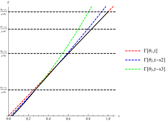
  Figure 12: Construction of $\Gamma$

  ∎

Appendix B Further applications

In this section we briefly outline alternate interpretations of Alibi or Fingerprint? developed in Section 4. This showcases a range of economic environments where “conclusive good news” (Fingerprint) and “conclusive bad news” (Alibi) is optimal among all dynamic persuasion strategies. We recall the setting of Alibi or Fingerprint?. There is a binary state space $\Theta=\{0,1\}$ and binary action space $A=\{0,1\}$. If the agent chooses $1$ at time $t$, her payoff is $v_{1}+f_{1}(t)$. If the agent chooses $0$ at time $t$, the principal’s payoff is $v_{0}+f_{0}(t)$. The agent’s payoff is $U(\mu,t)=\max\{\mu,1-\mu\}-c(t)$. $f_{0},f_{1},c$ are strictly increasing and differentiable.

An informed advisor (principal) is paid for her time, and chooses the flow of information to a decision maker (agent) who decides when to stop listening to the advisor, and which action to take. The advisor-decision relationship might concretely represent that of a prosecutor-jury as in Alibi or Fingerprint?, policy expert-public official, financial advisor-investor, and so on. The principal’s payoff comprises

• Contractible/monetary benefits: The principal is paid for her time at a rate $f(t)$ which is differentiable and strictly increasing. If the agent chooses action $1$, the principal is paid a lump-sum bonus of $\overline{b}>0$, and $0$ otherwise. The principal’s monetary benefits are capped at some level $M>\overline{b}$.

Optimality of Fingerprint-$t^{+}$

Assume for simplicity that $\overline{b}\geq M$ so that as long as the agent takes the principal’s preferred action, the principal hits her cap. Thus, the principal’s utility from the agent taking action $1$ at time $t$ is, and action $0$ at time $t$ are

$$\max\Big{\{}f(t)+\overline{b},M\Big{\}}=M\quad\text{and}\quad\max\Big{\{}f(t),M\Big{\}}$$

respectively. Translated into our framework, we have

$$v_{1}=M\quad f_{1}(t)=0\quad\text{and}\quad v_{0}=0\quad f_{0}(t)=\max\Big{\{}f(t),M\Big{\}}.$$

Note here we have $\Delta v+\Delta f\geq 0$ for all $t$ so the principal always prefers action $1$. From Corollary 4.2, it can be verified that

$$2\Psi_{1}^{+}(t^{{\dagger}})-\frac{f_{0}^{\prime}(t^{{\dagger}})}{c^{\prime}(t^{{\dagger}})}=\underbrace{(2e^{-c(t^{+})}-1)}_{=0}\frac{f^{\prime}_{0}(t)}{c^{\prime}(t)}=0$$

and furthermore, $f^{\prime}_{1}=0$ and $f^{\prime}_{0}\geq 0$ so the second condition for the optimality of Fingerprint-$t^{+}$ is fulfilled. Finally, note that for any $t^{+}\geq f^{-1}(M)$, $\Delta v+\Delta f(t^{+})=0$. A large $t^{+}$, in turn, corresponds to a sufficiently low waiting cost $c$ for the agent.

Optimality of Fingerprint-$\widehat{t}$

We now outline an example in which “preference reversals” are natural which then implies that conclusive good news which terminates at a non-degenerate stopping belief can be optimal. In particular, suppose that in addition to monetary benefits for the principal detailed above, she also suffers

• Non-contractible/non-monetary costs: If the agent chooses action $1$, the principal pays an extra non-monetary cost of $0<\underline{b}<\overline{b}$. This might represent the extra work if the agent chooses action $a=1$ e.g., if the client goes through with the project, the consultant has to execute it which requires additional effort on her part.

Translated into our framework, we have that the principal’s utility is

$$v_{1}=\overline{b}-\underline{b}\quad f_{1}(t)=\max\Big{\{}f(t),M-\overline{b}\Big{\}}\quad\text{and}\quad v_{0}=0\quad f_{0}(t)=\max\Big{\{}f(t),M\Big{\}}$$

noting now that $\Delta v+\Delta f<0$ for large enough $t$ so from Corollary 4.2 a conclusive good news persuasion strategy under which the agent stops at an inconclusive belief (e.g., Fingerprint-$\widehat{t}$) can be optimal.

References

- Aghion and Tirole (1997) Aghion, P. and J. Tirole (1997): “Formal and real authority in organizations,” Journal of political economy, 105, 1–29.
- Armstrong and Vickers (2010) Armstrong, M. and J. Vickers (2010): “A model of delegated project choice,” Econometrica, 78, 213–244.
- Arrow et al. (1949) Arrow, K. J., D. Blackwell, and M. A. Girshick (1949): “Bayes and minimax solutions of sequential decision problems,” Econometrica, Journal of the Econometric Society, 213–244.
- Ball (2023) Ball, I. (2023): “Dynamic information provision: Rewarding the past and guiding the future,” Econometrica, 91, 1363–1391.
- Bernheim and Ray (1989) Bernheim, B. D. and D. Ray (1989): “Collective dynamic consistency in repeated games,” Games and economic behavior, 1, 295–326.
- Che et al. (2013) Che, Y.-K., W. Dessein, and N. Kartik (2013): “Pandering to persuade,” American Economic Review, 103, 47–79.
- Che et al. (2023) Che, Y.-K., K. Kim, and K. Mierendorff (2023): “Keeping the listener engaged: a dynamic model of bayesian persuasion,” Journal of Political Economy, 131, 1797–1844.
- Che and Mierendorff (2019) Che, Y.-K. and K. Mierendorff (2019): “Optimal dynamic allocation of attention,” American Economic Review, 109, 2993–3029.
- Curello and Sinander (2022) Curello, G. and L. Sinander (2022): “The comparative statics of persuasion,” arXiv preprint arXiv:2204.07474.
- Ely et al. (2015) Ely, J., A. Frankel, and E. Kamenica (2015): “Suspense and surprise,” Journal of Political Economy, 123, 215–260.
- Ely (2017) Ely, J. C. (2017): “Beeps,” American Economic Review, 107, 31–53.
- Ely and Szydlowski (2020) Ely, J. C. and M. Szydlowski (2020): “Moving the goalposts,” Journal of Political Economy, 128, 468–506.
- Escudé and Sinander (2023) Escudé, M. and L. Sinander (2023): “Slow persuasion,” Theoretical Economics, 18, 129–162.
- Farrell and Maskin (1989) Farrell, J. and E. Maskin (1989): “Renegotiation in repeated games,” Games and economic behavior, 1, 327–360.
- Fudenberg et al. (2018) Fudenberg, D., P. Strack, and T. Strzalecki (2018): “Speed, accuracy, and the optimal timing of choices,” American Economic Review, 108, 3651–3684.
- Georgiadis-Harris (2021) Georgiadis-Harris, A. (2021): “Information acquisition and the timing of actions,” Tech. rep., Working Paper.
- Hart and Tirole (1988) Hart, O. D. and J. Tirole (1988): “Contract renegotiation and Coasian dynamics,” The Review of Economic Studies, 55, 509–540.
- Hébert and Woodford (2023) Hébert, B. and M. Woodford (2023): “Rational inattention when decisions take time,” Journal of Economic Theory, 208, 105612.
- Hébert and Zhong (2022) Hébert, B. and W. Zhong (2022): “Engagement maximization,” arXiv preprint arXiv:2207.00685.
- Henry and Ottaviani (2019) Henry, E. and M. Ottaviani (2019): “Research and the approval process: The organization of persuasion,” American Economic Review, 109, 911–955.
- Kamenica and Gentzkow (2011) Kamenica, E. and M. Gentzkow (2011): “Bayesian persuasion,” American Economic Review, 101, 2590–2615.
- Keller and Rady (2015) Keller, G. and S. Rady (2015): “Breakdowns,” Theoretical Economics, 10, 175–202.
- Keller et al. (2005) Keller, G., S. Rady, and M. Cripps (2005): “Strategic experimentation with exponential bandits,” Econometrica, 73, 39–68.
- Knoepfle (2020) Knoepfle, J. (2020): “Dynamic Competition for Attention,” Tech. rep., University of Bonn and University of Mannheim, Germany.
- Koh and Sanguanmoo (2024) Koh, A. and S. Sanguanmoo (2024): “Attention capture,” arXiv preprint arXiv:2209.05570.
- Liang et al. (2022) Liang, A., X. Mu, and V. Syrgkanis (2022): “Dynamically Aggregating Diverse Information,” Econometrica, 90.
- Luenberger (1997) Luenberger, D. G. (1997): Optimization by vector space methods, John Wiley & Sons.
- Morris (2001) Morris, S. (2001): “Political correctness,” Journal of political Economy, 109, 231–265.
- Moscarini and Smith (2001) Moscarini, G. and L. Smith (2001): “The optimal level of experimentation,” Econometrica, 69, 1629–1644.
- Orlov et al. (2020) Orlov, D., A. Skrzypacz, and P. Zryumov (2020): “Persuading the principal to wait,” Journal of Political Economy, 128, 2542–2578.
- Renault et al. (2017) Renault, J., E. Solan, and N. Vieille (2017): “Optimal dynamic information provision,” Games and Economic Behavior, 104, 329–349.
- Sannikov and Zhong (2024) Sannikov, Y. and W. Zhong (2024): “Martingale embeddings: theory and applications,” Working paper.
- Siegel and Strulovici (2020) Siegel, R. and B. Strulovici (2020): “The economic case for probability-based sentencing,” Tech. rep., Working paper.[132].
- Smolin (2021) Smolin, A. (2021): “Dynamic evaluation design,” American Economic Journal: Microeconomics, 13, 300–331.
- Steiner et al. (2017) Steiner, J., C. Stewart, and F. Matějka (2017): “Rational inattention dynamics: Inertia and delay in decision-making,” Econometrica, 85, 521–553.
- Strulovici (2017) Strulovici, B. (2017): “Contract negotiation and the coase conjecture: A strategic foundation for renegotiation-proof contracts,” Econometrica, 85, 585–616.
- Wald (1947) Wald, A. (1947): “Foundations of a general theory of sequential decision functions,” Econometrica, Journal of the Econometric Society, 279–313.
- Zhao et al. (2024) Zhao, W., C. Mezzetti, L. Renou, and T. Tomala (2024): “Contracting over persistent information,” Theoretical Economics, 19, 917–974.
- Zhong (2018) Zhong, W. (2018): “Information Design Possibility Set,” .
- Zhong (2022) ——— (2022): “Optimal dynamic information acquisition,” Econometrica, 90, 1537–1582.