Coupled heat and fluid transport in pulled extrusion of cylinders
Abstract
In the fabrication of optical fibres, the viscosity of the glass varies dramatically with temperature so that heat transfer plays an important role in the deformation of the fibre geometry. Surprisingly, for quasi-steady drawing, with measurement of pulling tension, the applied heat can be adjusted to control the tension and temperature modelling is not needed. However, when pulling tension is not measured, a coupled heat and fluid flow model is needed to determine the inputs required for a desired output. In the fast process of drawing a preform to a fibre, heat advection dominates conduction so that heat conduction may be neglected. By contrast, in the slow process of extruding a preform, heat conduction is important. This means that solving the coupled flow and temperature modelling is essential for prediction of preform geometry. In this paper we derive such a model that incorporates heat conduction for the extensional flow of fibres. The dramatic variations in viscosity with temperature means that this problem is extremely challenging to solve via standard numerical techniques and we therefore develop a novel finite-difference numerical solution method that proves to be highly robust. We use this method to show that conduction significantly affects the size of internal holes at the exit of the device.
keywords:
slender-body theory , low-Reynolds-number flows , heat transport[inst1]organization=School of Computer and Mathematical Sciences and Institute of Photonics and Advanced Sensing,addressline=The University of Adelaide, postcode=5005, state=SA, country=Australia
[inst2]organization=College of Science and Engineering,addressline=Flinders University, postcode=5042, state=SA, country=Australia
[inst3]organization=Department of Mathematics,addressline=City University of Hong Kong, city=Kowloon, country=Hong Kong SAR
[inst4]organization=Center for Applied Mathematics and Statistics,addressline=New Jersey Institute of Technology, city=Newark, postcode=07102, state=NJ, country=USA
1 Introduction
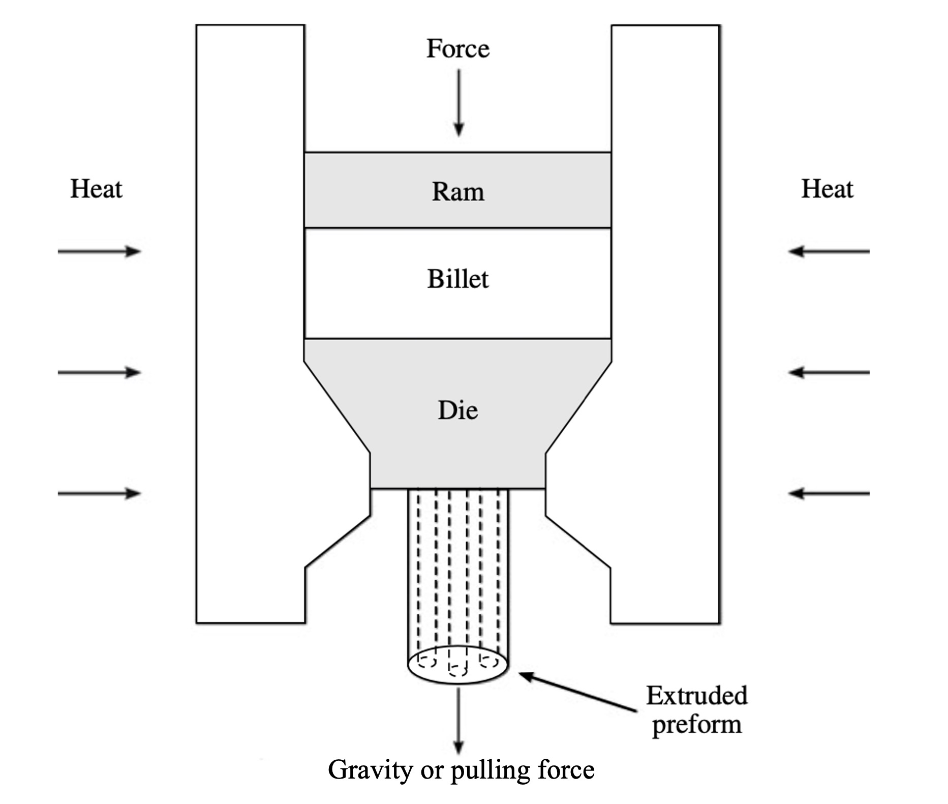
Microstructured optical fibres (MOFs) are optical fibres, typically 100-200 micrometers in diameter, with one or more internal air channels aligned with the fibre axis. MOF fabrication consists of the fabrication of a macroscopic version of the fibre having a diameter of one or more centimetres, called a fibre preform, followed by the drawing of this preform to a fibre. This paper focuses on fibre-preform fabrication by extrusion, whereby a billet of glass or polymer is heated and pushed through a die by a ram [1], as shown in Figure 1. The die has blockages that result in air channels (or holes) in the extruded preform [2]. The extruded preform may simply stretch under its own weight due to gravity or the lower end of the preform may be pulled at a prescribed speed. This paper focuses on pulled extrusion, which is similar to fibre drawing. However, in terms of the speed at which the glass moves, preform extrusion is many orders of magnitude slower than fibre drawing.
One of the main reasons that MOFs have become such an important new technology is that the hole structure can be designed to fabricate fibres that have very special optical properties. This is fundamental in a wide array of applications including communication networks [1], high-temperature and pressure sensors [4, 5, 6], chemical sensing [7, 8, 9], and biological sensing such as DNA detection [10, 11, 12]. Nevertheless, the optical properties can depend very sensitively on the geometry of the internal structure of the fibre and hence achieving very high tolerances in the manufacturing process is paramount. The internal structure undergoes deformation during both the extrusion and drawing stages, and the mechanisms that determine the changes in hole position and shape [2] are complicated and hence extremely careful modelling is required.
Temperature is an important factor that affects the deformation of the fibre because of the dramatic changes in viscosity with temperature that occur for the materials that are typically used. For the quasi-steady processes of fibre drawing and pulled extrusion, where the fibre material enters and exits the deformation region at fixed speeds, mass conservation dictates that the ratio of these speeds determines the change in cross-sectional area. Surprisingly, however, the pulling tension determines the change in the cross-sectional geometry of the thread [13]. The pulling tension depends on the temperature but, when this tension is measured, it can be controlled by adjusting the applied heat so that knowledge of the temperature profile in the thread is not needed to achieve a desired geometry change. Hence modelling of temperature through the deformation region is of limited importance when pulling tension is measured. However, where pulling tension is not measured (perhaps due to the fragility of the fibre or because the fabrication devices are not suitably equipped), temperature modelling becomes necessary. In the case of fibre drawing, the speed of the process means that advective heat transport is dominant and conduction can be assumed to be negligible [14]. By contrast, in the case of pulled preform extrusion (for which tension measurement is is atypical) the process is slower and both advective and conductive heat transport are important. To understand the effect of conduction in the deformation process, we must carefully model thermal effects to determine the initial geometry and conditions required to obtain a desired output. Developing such a model requires one to overcome a number of challenges including the complicated evolution of free boundaries, possible topological changes if holes close or merge, highly nonlinear dynamics due to dramatic viscosity changes and possible oscillatory instabilities.
The work on preform extrusion is not as extensive as that on fibre drawing. The existing mathematical model of preform extrusion is based on unsteady gravitational extrusion, for which Tronnolone et al. [3, 15] used a similar approach to Stokes et al. [13] to study extrusion of preforms with arbitrary hole geometries. However, their analysis only considers the isothermal case. In contrast to Tronnolone et al. [3, 15], this paper explores the quasi-steady pulled extrusion process and couples flow with energy transport.
There has been a significant amount of work done on modelling of the fibre drawing process which is relevant to pulled extrusion. The first model of drawing of axisymmetric solid thread was performed by Matovich and Pearson [16], assuming isothermal flow. Dewynne et al. [17] provided the systematic derivation of an asymptotic model for fibre drawing of non-axisymmetric fibres with isothermal flow. They showed that the cross-sectional shape of fibre changes only in scale in the absence of surface tension. This approach was extended to include inertia and gravity by Dewynne et al. [18]. Then, Cummings and Howell [19] developed an isothermal, non-axisymmetric model for solid threads with surface tension. This work was extended to model an annular, non-axisymmetric thin walled tube by Griffiths and Howell [20, 21].
Fitt et al. [22] modelled the drawing of axisymmetric tubes in a non-isothermal setting. They considered that axial energy transport is dominated by advection, and neglected conduction. Non-isothermal drawing of non-axisymmetric tubes, also neglecting conduction, was considered by Griffiths and Howell [21]. Taroni et al. [23] performed a very detailed exploration of non-isothermal drawing of axisymmetric fibres; they neglected surface tension and also obtained an energy equation that neglects axial conduction. He et al. [24] considered non-isothermal axisymmetric drawing of threads, with temperature-dependent viscosity and surface tension. Again, advection was considered while conduction was neglected.
The drawing of fibres with arbitrary hole structures was modelled by Stokes et al. [13], decoupling the axial and transverse flows and generalizing the results of Griffiths and Howell [21] to the case of multiple holes. However, they considered a prescribed axially varying viscosity but did not explicitly model the temperature. Rather they showed that the harmonic mean of the viscosity through the neck-down region determines the final fibre geometry, with the temperature to achieve this obtained by pulling with the required tension. The effect of adding pressure within air channels through the fibre was modelled by Chen et al. [25]. The recent work of Stokes et al. [14] coupled a temperature model to the flow model for drawing non-axisymmetric threads with arbitrary geometry. The temperature model considers only advection and neglects conduction.
This paper considers an arbitrary cross-sectional geometry but unlike all the above-mentioned studies includes the effects of axial conduction that are important in extrusion processes. In fibre drawing, both applied heating and cooling are important [14], but for preform extrusion the glass is hot when it exits the die and then cools down below it. Hence, we focus on external cooling.
Having derived the model, we explain why it is extremely challenging to solve using standard numerical techniques. We hence develop a bespoke numerical method that is highly robust. We use this to consider the axisymmetric case and show that conduction can have a significant effect on the hole size at the exit of the device.
2 Model formulation
2.1 Full model
A schematic diagram of the pulled extrusion process is shown in Figure 2. The spatial coordinates are , with the axis directed along the axis of the preform from the die exit at , is time, the velocity vector is , pressure is , and temperature is . We define to be the square root of the cross-sectional area at position and time . The preform exits the die and enters the flow domain with cross-sectional area , temperature , axial speed , and a specified cross-sectional geometry. Below the die the preform cools and also stretches because it is pulled at a point sufficiently far from the die exit at a speed . The ratio is known as the “draw ratio”. We assume that at axial position the preform is sufficiently cool, and the viscosity sufficiently large, that there is no significant deformation beyond this point. Thus the problem is quasi-steady and the evolution of the geometry can be modelled over the spatial domain , with .
As done by Stokes et al. [13, 14], Tronnolone et al. [15], and Tronnolone [26], we assume the glass to be an incompressible Newtonian fluid modelled by the continuity and Navier-Stokes equations
| (1a) | ||||
| (1b) | ||||
where the fluid has constant density , temperature-dependent viscosity , and is the stress tensor. We denote the location of the outer boundary by and the location of the boundaries of the inner holes by for . Then, the dynamic and kinematic boundary conditions are
| (2a) | |||
| (2b) | |||
where is the (constant) surface tension, is the local curvature of boundary , and
is the outwards pointing normal vector on . We denote the entire boundary by . We also define to be the total boundary length of the cross-section at position and time , where is the length of the external cross-sectional boundary and is the boundary length of the th hole in the cross-section.
Note that the viscosity of glass is strongly dependent on temperature. However, surface tension is only weakly dependent on temperature [27, 28, 29], and so, is here assumed to be constant. In this paper we also assume zero air pressure in the internal channels since to our knowledge pressurization of air channels is not used in extrusion of fibre preform.
The temperature in the glass is modelled by
| (3) |
where is the specific heat capacity and is the conductivity of the glass, both assumed to be constant. On the external boundary we assume both radiative and convective (Newton) cooling, while on internal boundaries we assume no heat flux, giving the boundary conditions
| (4a) | ||||
| (4b) | ||||
The parameter is the Stefan–Boltzmann constant, is the surface absorptivity/emissivity, and is the convective heat transfer coefficient. The initial temperature of the preform is denoted by , which is the temperature at . The (constant) ambient air temperature is denoted by . At large distance from the inlet, the glass temperature must equilibriate with the ambient and hence
Typical values for all physical parameters are given in Table 1. Note, however, that the values of and differ from one device to another and can be somewhat challenging to estimate.
| Parameter | Symbol | Approx. value | Units |
|---|---|---|---|
| Specific heat | 557 | ||
| Conductivity | 0.78 | ||
| Density | 3600 | ||
| Stefan–Boltzmann constant | |||
| Surface absorptivity/emissivity | 0.8 | - | |
| Convective heat transfer coefficient | 95 | ||
| Ambient air temperature | 290 | K | |
| Surface tension | 0.24 | ||
| Initial temperature | 970 | K | |
| Viscosity at temperature | Pa s | ||
| Preform cross-sectional area | |||
| Draw ratio | - | ||
| Length | 0.2 | m | |
| Feed speed |
In addition we require a viscosity–temperature function , which, in this paper, is assumed to be of the form used by He et al. [24],
| (5) |
where is the viscosity at the initial temperature , and is the constant that governs the sensitivity of the viscosity to temperature. This exponential law models the dramatic changes that occur in viscosity during the cooling process.
2.2 Non-dimensionalisation
We non-dimensionalise the equations using a similar approach to that of Stokes et al. [14]. The axial position is non-dimensionalised by the typical length over which the preform deforms, whereas the transverse variables are non-dimensionalised using that represents the square root of the initial cross-sectional area. We define the slenderness parameter to be the ratio of the transverse length scale to the axial length scale,
| (6) |
and assume a slender preform, so that . The dimensionless variables, denoted by primes are,
| (7) | |||
The dimensionless form of the viscosity–temperature function (5) is
| (8) |
where .
We now use these scalings to non-dimensionless our problem. Also, because it is quasi-steady, we assume time independence. The continuity equation becomes
| (9) |
while the momentum equation (1b) yields
| (10a) | |||
| (10b) | |||
| (10c) | |||
where
| (11) |
is the Reynolds number. Similar non-dimensionalisation of the dynamic boundary condition (2a) gives
| (12a) | |||
| (12b) | |||
| (12c) | |||
where
| (13) |
is the capillary number, and the kinematic boundary conditions (2b) become
| (14) |
We also have the boundary conditions at and at .
Finally, non-dimensionalising the temperature equation (3) and assuming no time dependence gives
| (15) |
where
| (16) |
is the Péclet number. The boundary conditions (4a) and (4b) become
| (17a) | |||
| (17b) | |||
where
| (18) |
These equations are similar to those of Stokes et al. [14] but differ in that our problem has no initial heating region, just cooling below the die exit at where the temperature is at its maximum value . As we have .
2.3 Asymptotic model
We next make use of the smallness of the slenderness parameter to obtain an asymptotic model. Details of the derivation process are similar to those given in [14] and we here just give a brief outline and refer the reader to [14] for details.
First, all dependent variables are expanded in powers of
| (19) |
with similar expansions for , , , , , , , and . These asymptotic expansions are substituted into the equations of section 2.2 and equations at each order of are obtained.
It is readily shown [14] that the leading-order temperature and velocity are independent of the cross-sectional coordinates, i.e.
Furthermore, the leading-order conservation equation integrated over the cross-section at axial position , together with the leading-order kinematic condition integrated over the cross-section boundary and a transport theorem from Dewynne et al. [17], give
| (20) |
for any axial position .
Then, considering the terms of the momentum equation (10a), integrating over the cross-section at axial position , and using the divergence theorem, the terms of boundary condition (12a), a transport theorem given by Dewynne et al. [17], and the conservation equation (20), we obtain the leading-order axial-flow equation
| (21) |
where is the total leading-order boundary length of the cross-section at position . This may be integrated with respect to and further manipulated to yield
| (22) |
where is the pulling tension.
In a similar manner we obtain the leading order temperature equation
| (23) |
Here is the leading-order length of the external boundary of the cross-section at axial position .
The above equations must be solved subject to boundary conditions , , and . The tension parameter must be chosen to satisfy .
The leading-order boundary lengths and , appearing in (21), (22) and (23), must be obtained from a transverse flow model describing how the cross-sectional geometry changes with . As described in [13, 14], using appropriate scalings and variable transformations, this can be written as a classical 2D Stokes-flow problem with unit coefficient of surface tension in a domain of unit area which gives the geometry evolution from some arbitrarily shaped initial geometry at to the final geometry at . However, for simplicity, in this paper we consider extrusion of an axisymmetric tube having an annular cross-section.
We define to be the (leading-order) outer radius of the preform and to be the (leading-order) ratio of the internal radius to the external radius, so the internal radius is defined as . Therefore, the cross-sectional area is given by
| (24) |
Although the deformation can be described in terms of and we choose to follow Stokes et al. [13, 14], and describe it in terms of and , where is the (leading-order) wall thickness of the cross-section. Then, using (24), we have
| (25) |
the wall thickness scaled with (or the wall thickness of an annulus with unit cross-sectional area). The scaled wall thickness is constrained by the condition . The value corresponds to the wall bursting () and is the minimum value of , whereas the maximum value corresponds to the hole closing (). It is readily shown that the length of the external cross-sectional boundary is
| (26) |
and the total cross-sectional boundary length is
| (27) |
The leading-order transverse-flow model in [13, 14] is derived using a transformation from the axial coordinate to a Lagrangian-like variable identifying a fluid cross-section, and all differential equations are then written in terms of this variable. In this paper, however, because we are considering only extrusion of axisymmetric tubes, we have, for simplicity, chosen to retain the Eulerian coordinate , in terms of which it is readily shown that is given by the differential equation
| (28) |
From this point on, the zero subscripts denoting the leading-order terms and the primes on dimensionless variables will, for convenience, be dropped.
2.4 The model as a system of first-order ODEs
Our model is a system of coupled ordinary differential equations (ODEs) for , , and , namely (22), (23), and (28); each equation involves all three dependent variables. Using typical physical parameter values from Table 1 we find that the Reynolds number (11) is very small, , which justifies neglect of the inertial term in (22).
Previous work [14, 23] on fibre drawing assumed a large Péclet number, enabling neglect of the second-order term in the temperature equation. Here, because we are concerned with the much slower process of preform extrusion, we assume so that energy conduction, as well as advection, is important. Thus, we have a second-order ODE for coupled with two first-order ODEs for and . Hence, we write the second-order temperature equation as two coupled first-order ODEs. To do this we define
which leads to the system of equations
| (29a) | ||||
| (29b) | ||||
| (29c) | ||||
| (29d) | ||||
We ensure that does not exceed its maximum value of by requiring its gradient to be zero once this value is reached. We assume the value of since this would represent breaking of the thread, which is not a desirable extrusion outcome.
We need to solve this system of equations over the domain where deformation occurs. The boundary conditions at are given by
| (30) |
We also have the condition where as . However, because our solution domain is, necessarily, finite, we must replace this with a condition at . We choose to use the condition at this boundary, equivalently . Although not strictly accurate, the assumption of a zero gradient is expected to lead to small error as long as the glass has cooled sufficiently and the viscosity has become sufficiently large that there is negligible deformation beyond . In addition we also must choose the tension parameter in (29a) so as to satisfy the draw ratio at . Therefore, the boundary conditions at are given by
| (31) |
3 Numerical solution method
While the above system of equations may appear straightforward to solve, this is far from the case. The retention of heat conduction in the problem results in a second-order derivative of temperature in the equations which, in turn, makes the system challenging to solve numerically. The essential reason for this is that the temperature equation (23) admits solutions that grow exponentially with . A rapid growth in temperature has a significant nonlinear effect on the viscosity. This is because the viscosity has the form (8) and so it varies dramatically with temperature and this means that the solution is very sensitive. Of course, a rapid increase in temperature is not physically meaningful for our problem, in which the glass cools, so that rapid growth of temperature must be eliminated/controlled by the boundary condition on at .
One might think that this problem can be attacked by using a shooting method, formulating the problem as an initial value problem and searching for an initial value (equivalently at ) that yields the required boundary condition at , i.e. . However, for typical choices of the temperature grows exponentially and the nonlinear coupling via the viscosity causes serious numerical problems. Thus, a shooting method is not appropriate.
One might also think the problem would be readily solved using a boundary value problem solver (for example, Matlab solvers bvp4c, bvp5c), However, these routines require initial guesses for the unknown variables and for the reasons explained above the solution is extremely sensitive to these. Hence, this too is deemed to be an unsatisfactory solution method.
In place of these methods we have devised a novel iterative finite difference numerical solution scheme that suppresses the unphysical growth in temperature. We discretise our spatial domain with uniformly spaced gridpoints, , , such that is the separation between any two consecutive gridpoints. We define as the value of at gridpoint , and similarly for , and . Then, noting that , and are known from the boundary conditions at , we discretise the differential equations for , and using the well-known forward-Euler method, enabling the next iterate of each of these unknown functions to be computed at each grid point step-by-step from to (left to right), starting with the known value for and ending with . Previous iterates of the dependent variables are used as required.
Equation (29c) for , however, has a boundary condition at , i.e. the value is known. Therefore, we discretise (29c) using the backward-Euler method. Usually the discretised equation would be seen as an implicit equation for determining from . However, we rearrange it to give an explicit equation for , assuming known values or previous iterates for the dependent variables at . Thus we compute in the reverse direction from right () to left (), starting with the known value and ending with . This is a non-conventional technique but works well for our problem, and enables the boundary condition at to be easily included.
We thus obtain the following system of difference equations to be iteratively evaluated for a given tension until the change in the dependent variables becomes less than some required tolerance:
| (32a) | ||||
| (32b) | ||||
| (32c) | ||||
| (32d) | ||||
where a supercript denotes the previous iterate of a variable.
Our numerical finite-difference method is illustrated in Figure 3. A Gauss-Seidel iterative scheme is employed, making use of updated values of variables as soon as they are known, so that only previous iterates of and are required. To start the iterative process, initial guesses for these are needed and these were chosen as and . In addition we require the boundary conditions,
| (33) |
For robustness, we solve the equations in the order given in (32). In particular, it is important to include the boundary condition at by solving for before solving for . Solving for before can result in numerical difficulties when solving for . To test for convergence, we compute the magnitude of the difference between two consecutive iteratives for each dependent variable and require that the maximum of these be less than a chosen tolerance value. The tolerance value was set at , giving a good balance between speed and accuracy of the solution.
Finally, the above procedure was written as a function to be used with Matlab’s root-finding routine ‘fzero’ so as to find the tension corresponding to a desired draw ratio .
4 Results
In this paper we focus on the importance of conductive heat transport in the pulled extrusion process, as quantified by the Péclet number . In the limit , the second-order term in the temperature equation may be neglected, reducing it to first-order. We will explore how different values of affect the solution. When the second-order term in the temperature equation is neglected we describe the coupled energy and flow extrusion problem as the “first-order problem”; otherwise it is described as the “second-order problem”. Below we will, at times, use subscripts on quantities , where denotes the quantity as given by solving the first-order problem and denotes the quantity as given by solving the second-order problem.
Aside from the Péclet number, all other parameters are set to fixed values. We choose the constant in the dimensionless viscosity-temperature function (8). This parameter governs the sensitivity of the viscosity to temperature and depends on the glass and the temperature range in the extrusion process. In practice, this value could be significantly larger. We further choose a representative draw ratio , initial aspect ratio (equivalently ), and dimensionless ambient air temperature . We also assume unit heat transfer coefficients and capillary number, i.e. , , . For investigations of these last three parameters see [31].
To determine the number of grid points for our finite-difference discretisation, such that our solution is sufficiently accurate, we computed solutions for two different values of the Péclet number, , for different values of . Figure 4 shows the temperature , aspect ratio , and pulling tension versus . As seen there, the second-order solution converges as increases; increasing from to gives changes to these quantities in the fourth and fifth decimal places. Therefore, we choose , which provides a good balance between accuracy and computational cost.
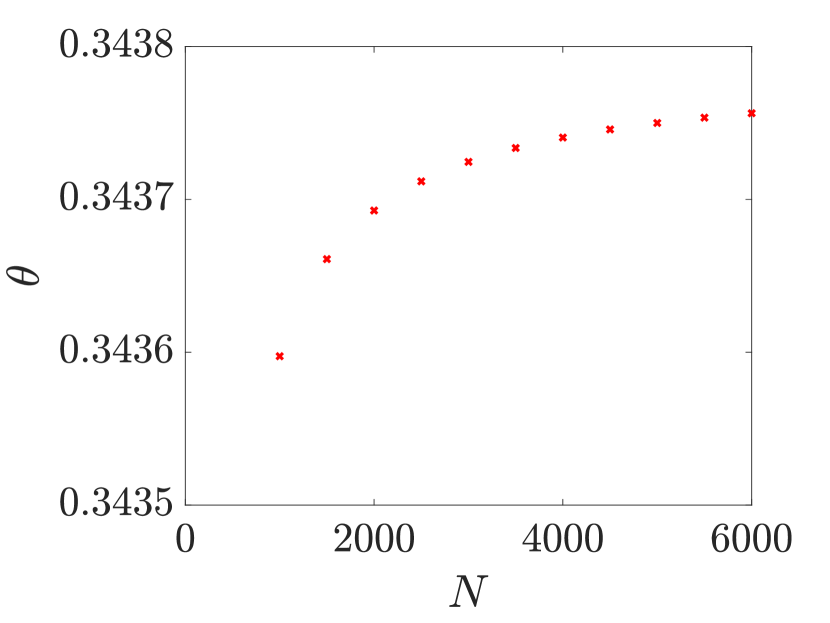
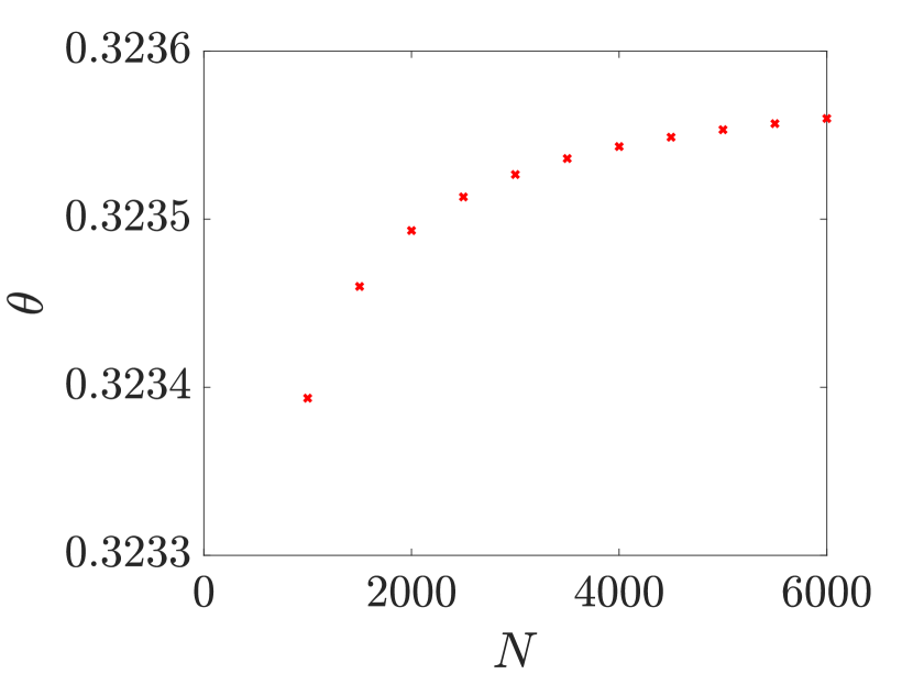
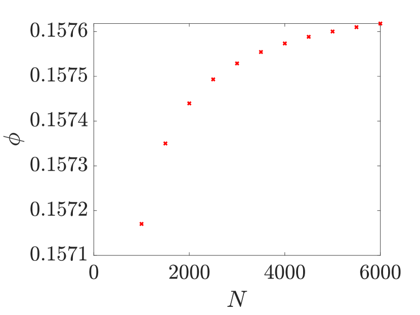
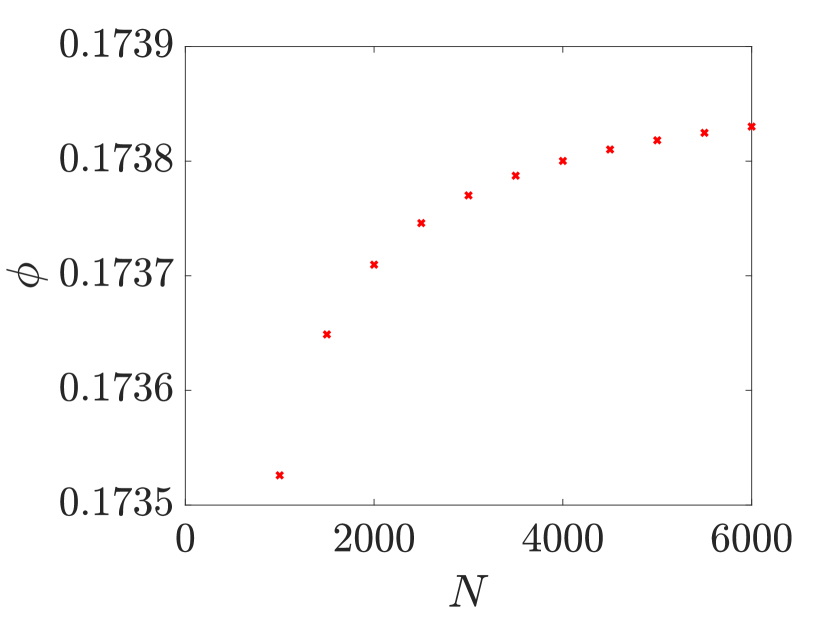
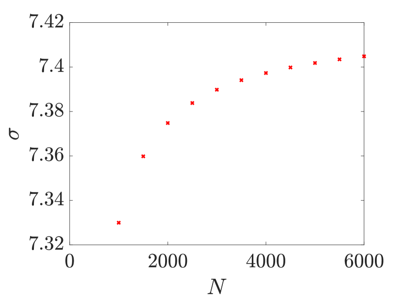
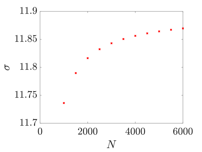
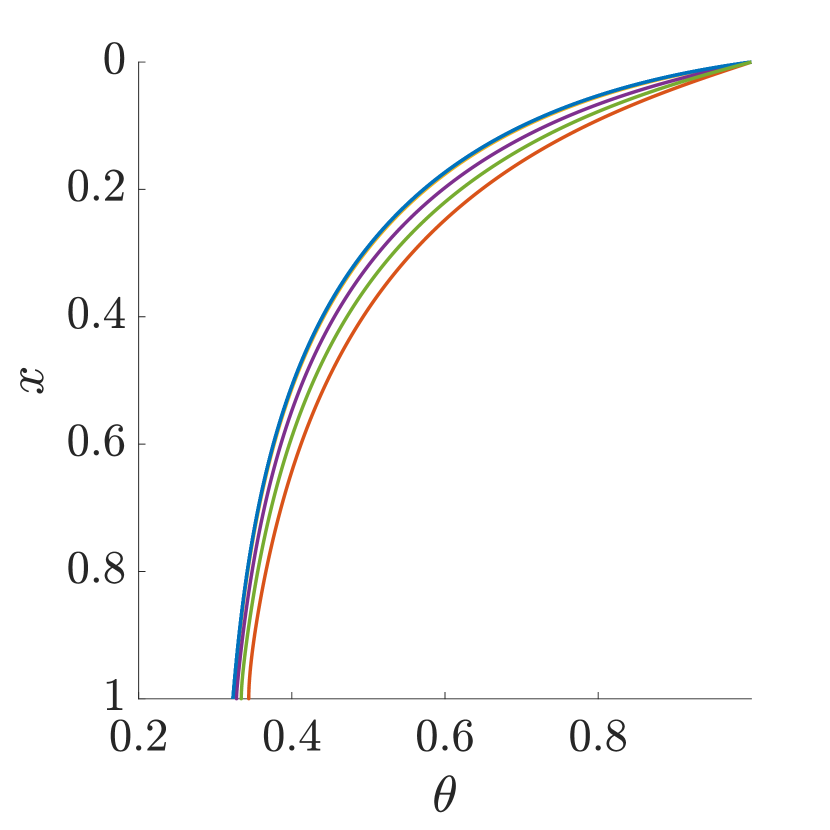
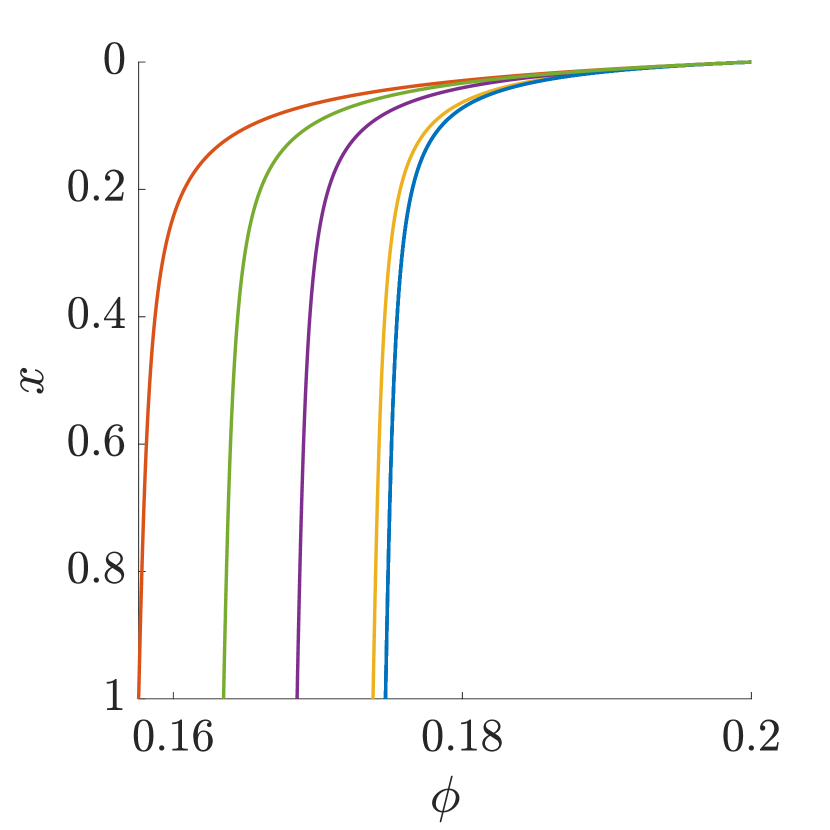
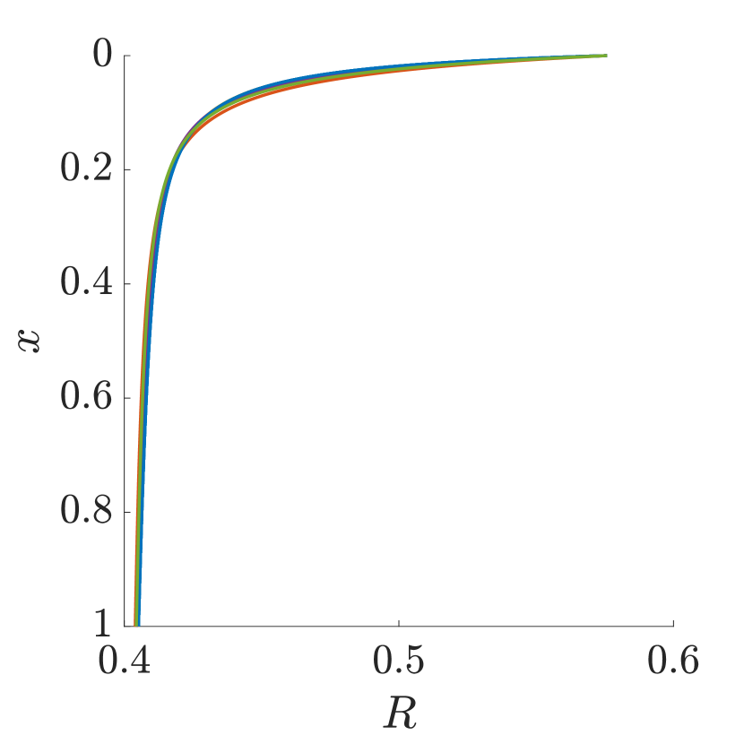
Figure 5 shows the temperature , aspect ratio , and external radius of the tube plotted against for (blue), (red), (green), (purple), and (yellow). The temperature of the first-order problem (blue curve) is quite different from the second-order problem with lowest Péclet number, as shown by the red curve in Figure 5(a). However, as the Péclet number increases to 600 (yellow curve), the second-order solution approaches the first-order solution. Figure 5(a) shows that heat conduction in the second-order problem with low Péclet number results in a higher temperature at . Indeed, for , the temperature throughout the glass is higher than for large Péclet number. This is due to the reciprocal of the Péclet number being the coefficient of the conduction term. When the Péclet number is small, the conduction of heat in the glass is important, increasing the glass temperature.
For the aspect ratio , we again see in Figure 5(b) that the yellow curve (second-order solution with ) and blue curve (first-order solution) are very similar. However, the red, green, and purple curves show to be significantly smaller for the smaller values of over the domain , with increasing as increases. The red curve corresponds to the second-order solution with lowest Péclet number, , and shows that heat conduction has a significant effect on the geometry. This relates to the higher glass temperature in this case, resulting in more deformation and hence a thicker wall and a smaller aspect ratio at any .
The external radius in Figure 5(c) decreases as increases. This is due to the thinning of the glass when it is pulled to achieve a draw ratio of . There is not, however, much difference between the three solution curves for ; this is because the pulling tension has been varied to achieve the same draw ratio for all three cases. Again, as the Péclet number increases from 10 (red curve) to 600 (yellow curve), the second-order solution approaches the first-order solution (blue curve).

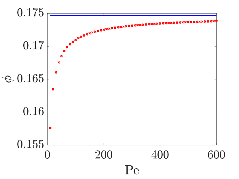
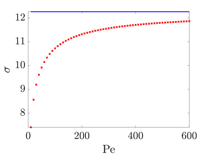
Figure 6 shows the temperature and the aspect ratio , both at , as well as the pulling tension for Péclet number in the range . Figure 6(a) shows the temperature at , . The temperature solution of the second-order problem, (red crosses), decreases as the Péclet number increases, approaching the solution of first-order problem (), , as becomes large. This shows that one actually needs a rather large value of the Péclet number for the conduction terms to become negligible.
Both the aspect ratio at and pulling tension of the second-order problem increase as Péclet number increases, approaching the solutions of the first-order problem (), as shown in Figures 6(b) and 6(c) respectively. The pulling tension needed in the case of the second-order problem is lower than for the first-order problem, because of the higher temperature throughout the glass arising from inclusion of conductive heat transport. With higher temperature, the glass is less viscous and hence requires less tension to achieve the draw ratio of . Figure 6 also show that for low Péclet number, there is a significant difference between the first-order and second-order solutions, indicating the importance of the inclusion of the second-order heat conduction term.
5 Conclusion
This paper focuses on the coupling of temperature with fluid flow in the modelling of preform extrusion, an important first stage in the process for fabrication of many micro-structured optical fibres. Temperature is known to be an important factor that affects geometry in fibre fabrication. However, it has not before been included in preform extrusion modelling. Further, while temperature has been included in previous modelling of the drawing of a preform to an optical-fibre, this work has assumed that heat conduction is negligible compared to advective heat transport [14] because of the fast speed of the drawing process. Here we have examined the importance of axial heat conduction in the much slower extrusion process. For simplicity, we have considered quasi-steady pulled extrusion of an axisymmetric tube. Non-negligible conduction changes the temperature model from a first-order to a second-order differential equation.
The extrusion problem with inclusion of heat conduction proves to be extremely numerically sensitive when standard numerical techniques are applied. We hence developed a bespoke numerical procedure based on an iterative finite difference method. While forward-Euler finite-differencing was used to discretise the equations for most of the unknown variables, backward-Euler finite differencing was used for the differential equation for the temperature gradient. This was done to suppress non-physical exponential growth in the temperature and, we believe, is a novel solution method. This strategy might be used in other mathematically similar problems.
We have compared solutions of the system with a second-order temperature equation for different values of the Péclet number, . For , our temperature equation reduces to first order and, in line with this, our solution to the second-order problem approaches that of the first-order problem as became large, giving verification of our novel solution methodology. For small and even moderate Péclet number and a low draw ratio, we have demonstrated the importance of including heat conduction in the model.
Future work might consider adapting the model and solution method to extrusion of preforms of arbitrary geometry through use of the reduced time variable , as used in Stokes et al. [14]. This problem is expected to be amenable to solution using a similar numerical approach to that employed in this paper. Also, the inclusion of a temperature equation with both advective and conductive heat transport in unsteady gravitational extrusion is a topic for future exploration.
Finally we point out that the physical heat transfer parameter values and , that appear in the dimensionless heat transfer parameters and , are not quantities that can be directly measured experimentally. They are not material parameters but rather model parameters that depend on the physical extrusion setup. Both parameters need to be determined by comparison of model solutions with suitable experiments. This is an avenue for future work and, indeed, is needed to enable predictive modelling.
Credit authorship contribution statement
Eunice B. Yuwono: Methodology, Software, Validation, Formal analysis, Investigation, Data curation, Writing - original draft, Visualisation. Yvonne M. Stokes: Conceptualization, Methodology, Software, Writing - review & editing, Visualisation, Supervision, Funding acquisition, Project administration. Jonathan J. Wylie: Conceptualization, Writing - review & editing. Hayden Tronnolone: Conceptualization, Writing - review & editing, Supervision.
Acknowledgements
We would like to thank Professor Neville Fowkes, University of Western Australia, for his useful comments on this problem. YMS acknowledges the support of Australian Research Council grants LP200100541 and FT160100108, both of which provided funding for EBY. JJW was supported by the Research Grants Council of Hong Kong Special Administrative Region, China (CityU 11300720).
References
- Monro and Ebendorff-Heidepriem [2006] T. M. Monro, H. Ebendorff-Heidepriem, Progress in microstructured optical fibres, Annual Review of Materials Research 36 (2006) 467––495.
- Ebendorff-Heidepriem and Monro [2007] H. Ebendorff-Heidepriem, T. M. Monro, Extrusion of complex preforms for microstructured optical fibers, Optics Express 15 (2007) 15086––15092.
- Tronnolone et al. [2016] H. Tronnolone, Y. M. Stokes, H. T. C. Foo, H. Ebendorff-Heidepriem, Gravitational extension of a fluid cylinder with internal structure, Journal of Fluid Mechanics 790 (2016) 308–338.
- Monzon-Hernandez et al. [2006] D. Monzon-Hernandez, V. P. Minkovich, J. Villatoro, High-temperature sensing with tapers made of microstructured optical fiber, IEEE Photonics Technology Letters 18 (2006) 511–513.
- Osório et al. [2017] J. H. Osório, G. Chesini, V. A. Serrão, M. A. Franco, C. M. Cordeiro, Simplifying the design of microstructured optical fibre pressure sensors, Scientific Reports 7 (2017) 2990.
- Reja et al. [2022] M. I. Reja, L. V. Nguyen, L. Peng, H. Ebendorff-Heidepriem, S. C. Warren-Smith, Temperature-compensated interferometric high-temperature pressure sensor using a pure silica microstructured optical fiber, IEEE Transactions on Instrumentation and Measurement 71 (2022) 1–12.
- Li and Zhang [2021] L. Li, Y.-N. Zhang, Fiber-optic SPR pH sensor based on MMF–NCF–MMF structure and self-assembled nanofilm, IEEE Transactions on Instrumentation and Measurement 70 (2021) 1–9.
- Monro et al. [2010] T. M. Monro, S. Warren-Smith, E. P. Schartner, A. François, S. Heng, H. Ebendorff-Heidepriem, S. Afshar, Sensing with suspended-core optical fibers, Optical Fiber Technology 16 (2010) 343–356.
- Warren-Smith et al. [2009] S. C. Warren-Smith, H. Ebendorff-Heidepriem, T. C. Foo, R. Moore, C. Davis, T. M. Monro, Exposed-core microstructured optical fibers for real-time fluorescence sensing, Optics Express 17 (2009) 18533–18542.
- Bertucci et al. [2015] A. Bertucci, A. Manicardi, A. Candiani, S. Giannetti, A. Cucinotta, G. Spoto, M. Konstantaki, S. Pissadakis, S. Selleri, R. Corradini, Detection of unamplified genomic DNA by a PNA-based microstructured optical fiber (MOF) Bragg-grating optofluidic system, Biosensors and Bioelectronics 63 (2015) 248–254.
- Ermatov et al. [2020] T. Ermatov, J. S. Skibina, V. V. Tuchin, D. A. Gorin, Functionalized microstructured optical fibers: materials, methods, applications, Materials 13 (2020) 921.
- Nguyen et al. [2012] L. V. Nguyen, S. C. Warren-Smith, A. Cooper, T. M. Monro, Molecular beacons immobilized within suspended core optical fiber for specific DNA detection, Optics Express 20 (2012) 29378–29385.
- Stokes et al. [2014] Y. M. Stokes, P. Buchak, D. G. Crowdy, H. Ebendorff-Heidepriem, Drawing of microstructured fibres: circular and non-circular tubes, Journal of Fluid Mechanics 755 (2014) 176–203.
- Stokes et al. [2019] Y. M. Stokes, J. J. Wylie, M. J. Chen, Coupled fluid and energy flow in fabrication of microstructured optical fibres, Journal of Fluid Mechanics 874 (2019) 548–572.
- Tronnolone et al. [2017] H. Tronnolone, Y. M. Stokes, H. Ebendorff-Heidepriem, Extrusion of fluid cylinders of arbitrary shape with surface tension and gravity, Journal of Fluid Mechanics 810 (2017) 127–154.
- Matovich and Pearson [1969] M. Matovich, J. Pearson, Spinning a molten threadline. steady-state isothermal viscous flows, Industrial & engineering chemistry fundamentals 8 (1969) 512–520.
- Dewynne et al. [1992] J. N. Dewynne, J. R. Ockendon, P. Wilmott, A systematic derivation of the leading-order equation for extensional flows in slender geometries, Journal of Fluid Mechanics 244 (1992) 323–338.
- Dewynne et al. [1994] J. Dewynne, P. Howell, P. Wilmott, Slender viscous fibres with inertia and gravity, The Quarterly Journal of Mechanics and Applied Mathematics 47 (1994) 541–555.
- Cummings and Howell [1999] L. Cummings, P. Howell, On the evolution of non-axisymmetric viscous fibres with surface tension, inertia and gravity, Journal of Fluid Mechanics 389 (1999) 361–389.
- Griffiths and Howell [2007] I. Griffiths, P. Howell, The surface-tension-driven evolution of a two-dimensional annular viscous tube, Journal of Fluid Mechanics 593 (2007) 181–208.
- Griffiths and Howell [2008] I. Griffiths, P. Howell, Mathematical modelling of non-axisymmetric capillary tube drawing, Journal of Fluid Mechanics 605 (2008) 181–206.
- Fitt et al. [2002] A. D. Fitt, K. Furusawa, T. M. Monro, C. P. Please, D. J. Richardson, The mathematical modelling of capillary drawing for holey fibre manufacture, Journal of Engineering Mathematics 43 (2002) 201––227.
- Taroni et al. [2013] M. Taroni, C. Breward, L. Cummings, I. Griffiths, Asymptotic solutions of glass temperature profiles during steady optical fibre drawing, Journal of Engineering Mathematics 80 (2013) 1–20.
- He et al. [2016] D. He, J. J. Wylie, H. Huang, R. M. Miura, Extension of a viscous thread with temperature-dependent viscosity and surface tension, Journal of Fluid Mechanics 800 (2016) 720–752.
- Chen et al. [2015] M. J. Chen, Y. M. Stokes, P. Buchak, D. G. Crowdy, H. Ebendorff-Heidepriem, Microstructured optical fibre drawing with active channel pressurisation, Journal of Fluid Mechanics 783 (2015) 137–165.
- Tronnolone [2016] H. Tronnolone, Extensional and Surface-Tension-Driven Fluid Flows in Microstructured Optical Fibre Fabrication, Ph.D. thesis, School of Mathematical Sciences, University of Adelaide, 2016.
- Babcock [1940] C. L. Babcock, Surface tension measurements on molten glass by a modified dipping cylinder method, Journal of the American Ceramic Society 23 (1940) 12–17.
- Shartsis and Smock [1947] L. Shartsis, A. W. Smock, Surface tensions of some optical glasses, Journal of the American Ceramic Society 30 (1947) 130–136.
- Parikh [1958] N. M. Parikh, Effect of atmosphere on surface tension of glass, Journal of the American Ceramic Society 41 (1958) 18–22.
- Schott [2014] Schott, F2 optical glass datasheet, 2014. https://mss-p-009-delivery.stylelabs.cloud/api/public/content/4c96933ddb2a4a06adf062d635f0b35d?v=e4f43a42.
- Yuwono [2023] E. B. Yuwono, Mathematical modelling of fibre fabrication; coupling heat transport with fluid flow in extrusion, MPhil thesis, School of Computer and Mathematical Sciences, University of Adelaide, 2023.