Online Pareto-Optimal Decision-Making for Complex Tasks using Active Inference
Abstract
When a robot autonomously performs a complex task, it frequently must balance competing objectives while maintaining safety. This becomes more difficult in uncertain environments with stochastic outcomes. Enhancing transparency in the robot’s behavior and aligning with user preferences are also crucial. This paper introduces a novel framework for multi-objective reinforcement learning that ensures safe task execution, optimizes trade-offs between objectives, and adheres to user preferences. The framework has two main layers: a multi-objective task planner and a high-level selector. The planning layer generates a set of optimal trade-off plans that guarantee satisfaction of a temporal logic task. The selector uses active inference to decide which generated plan best complies with user preferences and aids learning. Operating iteratively, the framework updates a parameterized learning model based on collected data. Case studies and benchmarks on both manipulation and mobile robots show that our framework outperforms other methods and (i) learns multiple optimal trade-offs, (ii) adheres to a user preference, and (iii) allows the user to adjust the balance between (i) and (ii).
Index Terms:
Multi-Objective Decision Making, Active Inference, Formal SynthesisI Introduction
The demand for robots to autonomously perform hazardous and repetitive tasks is steadily increasing [1, 2]. Such tasks often involve multiple, possibly competing, quantitative objectives, e.g., time and energy, requiring optimization for trade-offs between the objectives, known as Pareto optimal. In unknown environments, like the Martian surface or civilian households, however, such quantities are often stochastic and unknown a priori. Fortunately, they are measurable and can be learned online. Then, the robot should make decisions to learn all optimal trade-offs, or focus on learning a single user-preferred trade-off. Although highly desirable, accomplishing both simultaneously is challenging since the trade-off selection must balance exploring unknown trade-offs with exploiting preferred trade-offs. This paper focuses on this challenge and aims to develop a framework that simultaneously (i) learns multiple optimal trade-offs, (ii) embeds an intuitive user preference over a desired trade-off, and (iii) allows the user to adjust the balance between (i) and (ii).
Example 1.
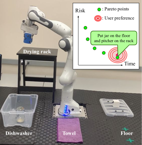
Consider the robotic dishwashing scenario in Figure 1. The robotic manipulator is equipped with a sampling-based motion planner (e.g., RRT and PRM [3, 4]) that solves A-to-B planning queries. The robot must repetitively complete a complex task of inserting the dishes into the dishwasher, then properly drying them by either placing directly up on the rack, or placing on the towel and moving them to the floor. In such a scenario, the robot should be both efficient (minimize the time of execution) and risk-aware when carrying fragile dishes high above the ground. However, due to the nature of sampling-based methods, the characteristics of actions (time and path-height) are unknown a priori, and hence the robot needs to construct accurate models of these quantities during deployment. The robot can either quickly place dishes up on a drying rack (low-time, high-risk for fragile objects), or manually dry dishes on the ground (high-time, low-risk). Considering a human user may prefer one trade-off over the other, the robot must both learn the quantitative models, and decide amongst optimal trade-off actions while adhering to the user’s preference. Such decision making problems involving competing objectives can be formulated as multi-objective reinforcement learning (MORL) [5, 6, 7, 8].
Embedding the satisfaction of a task into the multi-objective reward function often aims to capture both qualitative properties of the task (i.e. whether or not the robot completed the task), as well as quantitative properties (i.e. how well the robot completed the task) [9]. However, properly representing qualitative task completion through a reward function is a challenging problem, often requiring the use of methods such as inverse reinforcement learning (IRL) [10]. In uncertain environments, it is not always possible to obtain large amounts of human teaching data. Furthermore, these learning-based methods often fail to provide safety guarantees on the qualitative behavior of the robot. Nevertheless, in scenarios where qualitative aspects of the robotic model and task are known beforehand, e.g., manipulation problems, formal methods [11] provide alternative approaches to both task representation and plan synthesis using temporal logic specifications, such as Linear Temporal Logic (LTL) [12] and LTL over finite traces (LTLf) [13]. These planning methods can solve the qualitative portion of the learning problem and provide guarantees on the completion of tasks and safety while avoiding the need for IRL. Formal synthesis approaches have also been used to solve multi-objective quantitative planning problems [14]; however, those approaches assume a perfectly accurate quantitative model, which are often unavailable.
Unlike single-objective RL, MORL agents must select among potentially many optimal trade-offs. The numerical valuations of these optimal trade-offs are referred to as the Pareto front. The Multi-Objective Multi-Armed Bandit (MOMAB) community emphasizes learning all optimal trade-off actions, yielding valuable insight into the trade-off analysis of the learned results [15, 16, 17, 18]. Alternatively, one can use scalarization to convert the multi-objective problem into a single objective problem based on a preference trade-offs [5, 6, 7, 8]. Further description of these methods can be found in Sec. V. To the best of our knowledge, no MORL selection methods simultaneously propose mathematically sound adherence to a preferred trade-off while learning and exploring portions of the true Pareto front.
In light of these gaps, this study proposes a novel MORL framework centered around viewing optimal trade-off selection as its own high-level decision making under uncertainty problem. Specifically, we employ active inference (AIF), recently explored as a sound approach for sequential decision-making under uncertainty [19, 20, 21, 22] that minimizes an information-theoretic quantity known as surprise. We exploit the decision making power of AIF to adhere to a user’s ideal trade-off while exploring and learning localized portions of the whole Pareto front. This, however, introduces intractable computational complexity in optimizing for surprise for finite-horizon tasks. Our framework integrates multi-objective planning for a complex LTLf specification with high-level selection of an optimal trade-off by using a Bayesian approach to learning the quantitative model. We extend AIF to reasoning over finite horizon planning via upper-bounding the surprise with expected free energy (EFE). We derive computationally tractable techniques for optimizing EFE for LTLf tasks. Using our framework, we illustrate the performance trade-offs between biasing towards a user’s preferred Pareto point versus learning the entire Pareto front. Additionally, we showcase the utility of our approach using robotic case studies, including a hardware demonstration of the scenario in Example 1.
The major contributions of this work are three-fold:
-
•
A novel MORL framework that combines formally guaranteed task plan synthesis with efficient learning of Pareto-optimal behavior,
-
•
Derivation of a tractable approximation of a free energy formulation for finite horizon planning over an uncertain quantitative model,
- •
A detailed discussion on related work along with an overview of AIF are provided in Sec. V.
II Preliminaries and Problem Formulation
This paper studies a framework that enables a robot to (i) repetitively complete a given high-level complex task, and (ii) learn the most efficient and user-aligned means of completing the task. These two goals separate nicely into qualitative behavior, i.e., whether or not the robot completes the task, and quantitative behavior, i.e., how well the robot completes the task. We restrict our attention to problems where qualitative aspects of the model (i.e. robotic states, state transitions, task related observations, etc.) are known, but quantitative aspects (i.e. costs of executing robotic actions) are unknown and must be learned. Below, we first formally define a robot model and LTLf task specifications. We then connect these definitions with cost uncertainty and user preferences to be able to fully formulate the problem.
II-A Robot Model
We consider a robotic system modeled as a deterministic transition system (DTS), an abstraction used in many formal approaches to robotic systems, including both mobile robots and robotic manipulators [23, 24, 25, 26, 27, 28, 11]. To capture uncertainty in quantitative values, we augment classical DTS with a stochastic cost function as defined below.
Definition 1 (DTS-sc).
A labeled Deterministic Transition System with a stochastic cost function (DTS-sc) is a tuple , where
-
•
is a finite set of states,
-
•
is a finite set of actions,
-
•
is a deterministic transition function,
-
•
is a stochastic cost function that maps each state-action pair to an -dimensional probability distribution, where and is the set of all probability distributions over ,
-
•
is a set of atomic propositions related to the robot tasks, and
-
•
is a labeling function that assigns to each state the subset of propositions in that are true in .
A robot plan is a finite sequence of actions that induces a trajectory from a current state , where and, for all , . The observation of , denoted , is a trace where .
Example 2.
Consider a simplified DTS-sc model in Fig. 2 of the dishwashing scenario described in Fig. 1 with five states capturing the locations of each dish (: jar on floor, : pitcher on rack, etc.), and two actions load and unload. Each state observes either or . Each action from a state takes time and incurs some risk when transporting the jar, modeled with a unique multivariate cost distribution for each state-action pair.
When robot takes action at state , it endures distinct types of costs , e.g., energy expenditure and time of execution. This cost vector can generally be stochastic, i.e., the cost value of executing at can differ at different instances due to, e.g., changes in the environment or use of randomized algorithms (sampling-based planners). Hence, is a random variable whose distribution is given by , i.e., . With an abuse of notation, we use as the cost random variable for all state-action pairs, and hence .
We treat as a conditional distribution of a probabilistic transition-cost generative model, parameterized by the set of parameters , i.e.,
For ease of presentation, we denote specific parameters by such that .
We assume robot model is a Markov process. That is, for each state-action pair is independent, i.e., is independent from for all . Further, we assume each is a multivariate normal (MVN) distribution paramerized by a non-negative mean and covariance , i.e., . Note that this assumption allows for correlation between types of costs. For instance, if the execution of a robotic action takes a long time, it is likely that it also uses more energy.
In this work, we consider the realistic case where are unknown, i.e., both and are unknown for every . One of the goals of this work is to learn these parameters from data collected on during execution.
Given a plan and its induced trajectory , the cumulative cost of executing from state , denoted , is the sum of the state-action costs along , i.e., Since each is a random variable, is also a random variable, and its distribution is given by the convolution of the distributions, i.e.,
| (1) |
where is constructed by . Recall that is assumed to be a MVN; is also a MVN. Since true are unknown beforehand, we learn the parameters from experience. We denote the learned parameters by .
II-B Robotic Task
The robot is given a complex task that can be completed in finite time. To specify such tasks in a formal manner, we use Linear Temporal Logic over Finite Traces (LTLf) [13], which combine propositional logic with temporal operators.
Definition 2 (LTLf Syntax).
A Linear Temporal Logic over Finite Traces (LTLf) formula over is recursively defined as
where , (negation) and (conjunction) are Boolean operators, and (next) and (until) are temporal operators.
The commonly-used temporal operators “eventually” () and “globally” () can be defined as and , respectively.
The semantics of LTLf are defined over finite traces [13]. That is, an LTLf formula can be satisfied with a finite trace [13], denoted . We define the language of to be the set of finite traces that satisfy for the first time, i.e., let be the length of and for be the prefix of with length ; the language of is defined as
We say plan executed from satisfies if the resulting trace .
Example 3.
Following Example 2, we specify the task stating “the robot should first wash the dishes, and then dry the dishes.”
We want the robot to execute task repeatedly. Specifically, we are interested in synthesizing plans that episodically repeat . That is, once a plan is complete ( is satisfied), a new plan has to be synthesized from the current state to satisfy again. We assume that such a repetition is always physically possible for the robot, i.e., the robot always ends in a state from which there exists a plan that satisfies . For instance, in the above example, after drying dishes, the robot always ends in a state from which it can start washing a new pile of dirty dishes. Thus, we focus on the set of satisfying plans from every state, and refer to it as the -satisfying plan set.
Definition 3 (-Satisfying Plan Set).
Given DTS-sc robot model , state , and LTLf task formula , -Satisfying Plan Set is defined as
II-C Optimization Objectives
At each planning (decision) instance from state , we aim to select a plan that, in addition to completing task , optimizes for the expected cumulative cost . Since is -dimensional, it is in fact an -objective optimization problem. Moreover, the cost objectives may be competing, i.e., by optimizing one objective, another becomes sub-optimal. Hence, we want to optimize for the trade-offs between the objectives, which is known as Pareto optimal and best defined by the notion of vector dominance.
Definition 4 (Vector Dominance).
Let be two vectors and be the -th element of . Vector dominates , denoted by , iff for every and there exists an such that .
Definition 5 (Pareto Optimal).
For state and LTLf formula , plan is called Pareto optimal if
The set of all Pareto optimal plans from is denoted by . Then, for each , is called a Pareto point, and the set of all Pareto points is called the Pareto front, denoted .
At every planning instance (episode), we desire to select a Pareto optimal plan which ensures that the expected cost is not dominated by another plan. However, since are not available, it is impossible to compute for . Instead, we can use to compute a learned set of -satisfying Pareto optimal plans denoted . Similarly, let denote the set of expected cost vectors of each .
II-D User Preference
There are possibly many Pareto optimal plans that perform . We are interested in picking a plan that achieves the user’s most-preferred Pareto point in every instance. Given that our goal is autonomous operation, we require this preference to be provided as an input before deployment. This poses a challenge because the Pareto front is unknown a priori, and the user cannot know the exact Pareto point they prefer. Instead, as suggested in recent literature [29, 22], the user can provide a probability density function (pdf) that serves as an expressive way of capturing preferred observed outcomes. We extend this notion to the multi-objective domain, and leverage the expressive pdf preference as a tie-breaker between optimal trade-off candidates.
We specifically focus on user preference as a normal distribution over the objectives since it can be fully defined by only specifying a mean and covariance , respectively. Thus, by providing and , the user can not only express a desired trade-off region in the objective space, but also specify the willingness to explore alternative trade-offs (Pareto points) that allow the robot to learn more quickly, offering means to address the exploration-exploitation trade-off problem.
Example 4.
Suppose the dishwashing robot described in Fig. 1 is being deployed in a restaurant. If the restaurant is going to be busy, the user may define a preference distribution with mean in a low-time high-risk part of the objective space, whereas if the restaurant will be slow, the user may opt for a high-time, low-risk alternative, both of which can be informed by past observations of how humans wash the dishes. If the user is interested in learning other optimal trade-offs, or is uncertain how accurately they have estimated the mean, they can expand and orient the covariance around regions they would like the robot to explore information rich opportunities.
To meet user’s preference, we seek a Pareto point that is not “suprising.” The information theoretic definition of surprise is the negative log of model evidence [30]. Similarly, we define the surprise of an observation obtained by following a plan as:
| (2) |
This quantity can be derived by marginalizing the following generative model:
| (3) |
In active inference (AIF), one can inject a bias towards seeing certain outcomes by substituting the predictive outcome distribution with the prior preference (a.k.a. “evolutionary prior”) that is independent of any plan [31, 21]. We refer to the biased surprise as surprise w.r.t. :
| (4) |
In essence, under AIF, an agent acts to see desired observations. An overview of AIF is provided in Sec. V-B.
II-E Problem Statement
The problem we consider is as follows.
Problem 1.
Consider a DTS-sc robot model with unknown cost distributions, an LTLf task specification that the robot is to repeatedly complete, and a user preference distribution over cost objectives. Let denote the number of times (instances) the robot achieves task , and be the start state of the robot in the -th episode. Then, for each , synthesize a -satisfying plan such that
-
(i)
minimizes in (4),
-
(ii)
as , becomes Pareto optimal, i.e., , and
-
(iii)
as , the resulting Pareto front converges to the true Pareto front .
Note that, in Problem 1, satisfaction of (qualitative objective) at each instance is a hard constraint, and the optimization (quantitative) objectives in (i)-(iii) are soft constraints. Hence, by incorporating safety requirements in , safety satisfaction is guaranteed throughout the process. Furthermore, from the perspective of multi-objective decision making, Problem 1 is particularly challenging since adhering to a user’s preference and learning the Pareto front are arguably perpendicular efforts. In our approach, we address this challenge by using free energy minimization to naturally balance exploitation and exploration over the Pareto front.
III Approach
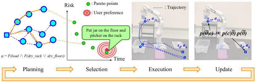
Our approach to Problem 1 is an iterative MORL framework with four phases: 1) planning Pareto optimal plans, 2) selection of the preferred Pareto optimal plan, 3) execution of the selected plan, and 4) update to the executed state-action cost parameters, as illustrated in Fig. 3. Planning, selection, and update all are dependent on the learning status of the robot. Hence, we start by formalizing our approach to modeling .
III-A Learning the Transition Cost Model
Recall that the cost of each is distributed as . However, are unknown and must be learned using experience. We take a Bayesian approach to learning by modeling with random variable . Specifically, we assume that the robot collects a realized sample drawn from each time is executed from . Let be the set of realizations of . We maintain a belief over using the Normal Inverse-Wishart (NIW) distribution, i.e.,
NIW is chosen because of the property of conjugacy for estimating unknown mean and covariance of a MVN distribution, i.e., the posterior is also represented analytically as a NIW [32]
Note that some works assume the covariance is known a priori [33], limiting the fidelity of the model. NIW strikes a balance between an over simplified parametric model (known covariance) and a sample inefficient non-parametric model [34]. We detail the the update procedure in Sec. III-D. If the user has an informed guess about the mean and covariance of a certain state-action distribution, they can set and respectively, reducing the number of decision making instances required to learn .
III-B Planning
At the start of each planning (decision-making) instance, we employ a multi-objective task planner to compute the set of approximate Pareto-optimal plans described in Def. 5. To this end, we formulate a correct-by-construction multi-objective shortest-path graph search problem, similar to [14], which can be solved with the following procedure.
III-B1 Product Graph Construction
An LTLf formula can be translated into a deterministic finite automaton (DFA) [13], a finite state-machine that precisely captures the language of .
Definition 6 (Deterministic Finite Automaton).
A DFA constructed from LTLf formula is a tuple where is a set of states, is the initial state, is the alphabet, is a deterministic transition function, and is a set of accepting states.
A trace induces a finite run on , where . Run is called accepting if . If is accepting, then trace is accepted by and satisfies , i.e., .
Using to capture the physical capability of the robotic system, along with to capture the temporal attributes of , we can construct a product automaton that intersects the restrictions of both and .
Definition 7 (Product Automaton).
Given a DTS-sc , current state , and DFA , a Product Automaton is a tuple , where
-
•
is a set of states,
-
•
, where , is the starting state in the current instance,
-
•
is the same action set in ,
-
•
is a transition function, where for states and and action , transition exists if and ,
-
•
, is a transition cost-vector function, and
-
•
is a set of accepting states.
Note that unlike stochastic cost function in , cost-vector function is not a distribution. We elaborate on further below.
Similar to , a plan induces a run on where . Run is accepting iff . Therefore, by construction, the set of -satisfying plans is equal to the set of all plans that induce paths on from to a .
III-B2 Transition Cost-Vector Function
We aim to define cost-vector function and accordingly formulate a multi-objective graph search problem on that enables the computation of the set of Pareto optimal -satisfying plans . Consider current state , plan , and induced path . Ideally, for every and , we want because the total cost of induced path becomes
Therefore, by assigning , the multi-objective Pareto front of the graph search problem on is exactly equal to (see Def. 5). Then, existing algorithms such as a multi-objective variant of Dijkstra’s algorithm or [35] can be employed to compute . Note that these multi-objective graph search algorithms are exponential in the worst case, however the average branching factor for a -dimensional vector belonging to a set of size , i.e. the set of all unique cost vector edge weights, is reduced to , with certain conditions on the ordering [35].
However, is unknown. A naive approach simply uses learned estimates for instead, but that suffers from biasing the solution towards taking transitions that have low estimate cost, regardless of how accurate is. To address this, we interweave exploration into the graph search problem, as detailed below.
III-B3 Pareto-Regret
The efficacy of learning can be analyzed with the notion of cumulative “Pareto-regret”, quantifying how sub-optimal each plan is with respect to the true Pareto front . Formally, given with true mean cumulative cost , the Pareto regret for a given instance is defined as
| (5) |
where is a vector of ones with appropriate dimension. Note that if , then . The cumulative regret up to instance is simply the summed regret for every instance, i.e. . To minimize cumulative regret, we augment the transition cost-vector with an exploration strategy.
III-B4 Pareto Cost-LCB
We adapt the well established Pareto-UCB1 [15, 36] strategy for computing an estimate Pareto front that balances the current best estimate cost model (exploitation) with a bonus reduction in cost (exploration). The learned mean transition-cost is calculated using the estimated parameters . To maintain optimality guarantees of the aforementioned graph search method, we rectify each element of to be non-negative. The cost-lower confidence bound (LCB) cost vector is computed element-wise as:
where is a “confidence” hyperparameter, is the current global time step across all decision instances, and is the number of times action has been executed from state .
Note that many multi-objective multi-armed bandit confidence bound approaches provide theoretical regret bounds that are logarithmic with respect to the number of decision instances. It is not straight forward to extend these regret bounds to this framework due to the exponential nature of the planning space which has size . Hence, we leave theoretical regret bounds to future research.
Using the techniques described above, we can now compute the approximate set of Pareto optimal plans while accounting for exploration of the environment. The exploration in planning aids in the effort in addressing goals (ii) and (iii) of Problem 1, however, to uphold proper learning of the Pareto front (iii), the selection must also explore among trade-offs.
III-C Pareto Point Selection
For the selection problem, one can think of candidate plans computed by the planner as abstract macro-actions, such that high-level decision making can be done sequentially for each instance. Fig. 4 provides a visual representation of the abstracted selection problem with respect to the evolution of the robotic system over each instance.
As described in Sec. II-D, ideally, the agent should select an action minimizing the surprise of outcomes. However, since it is analytically intractable to marginalize the joint distribution to derive the surprise, its upper bound, i.e., free energy, is minimized. Yet, the outcomes cannot be observed until a plan is actually executed, thus, the agents end up minimizing the so-called expected variational free energy (EFE) in active inference based decision-making. In this Pareto point selection problem, the EFE is described as follows (see Appendix A for detailed derivation).
| (6) |
where represents a proposal distribution. EFE is a variational quantity [37], yielding freedom in the choice of proposal distribution . As more closely resembles , the upper bound on (expected) surprise decreases. The first term of EFE in (III-C) represents how much the predicted cost distribution aligns with (i.e. exploitation), and the second and third terms represent how much the uncertainties of and can be reduced by following and measuring (i.e. exploration). Since the user does not know the true Pareto-optimal region a priori, EFE cannot be used to scalarize any plan in , as it may often be sub-optimal. Therefore, as described in Sec. V-A, the preferred plan is not guaranteed to also be an element in and vice versa. Consequently, in order to ensure that the user’s preference does not bias the system away from optimal behavior, this preference is only expressed over Pareto-optimal candidates. So, is scalarized via EFE in order to adhere to and reduce uncertainties in the belief over . Since models deterministic transitions, the second term of (III-C) can be ignored. Expanding the third term of (III-C) yields
| (7) |
where represents the entropy of a pdf. Then, the preferred plan is
| (8) |
Due to the Markov property of DTS-sc and (1), and of the convolved distribution are parameterized by and of each cost distribution respectively. According to the estimate transition cost model, are random variables themselves; therefore,
| (9) |
As described in Section III-A, each is a unique NIW, which makes (9) analytically intractable. To enable computation for in (8), we leverage both the functional freedom in choosing proposal distributions as well as three statistical approximations of (III-C): certainty equivalence of the predicted observation distributions [38], central limit theorem (CLT) [39], and Monte Carlo sampling [40].
III-C1 Approximating the First Term of (III-C)
Recall is the belief over parameters of the predicted observation distribution . To address the intractability, we can extract the current estimate parameters . This certainty-equivalence approximation makes a simple multivariate normal distribution
| (10) |
The first term can then be calculated as follows
| (11) |
where and are the mean vector and the covariance matrix of the user’s preference distribution (see Appendix B for detailed derivation).
III-C2 Calculating the Second Term of (III-C)
The convolved distribution is analytically intractable. However, we can leverage the CLT to determine a suitable proposal distribution that closely models . Since each is NIW-distributed, both the mean and variance are well-defined when and . Therefore, under the CLT, tends towards a MVN distribution as the plan length becomes large [41].
Consider the following vectorization of the parameters
| (12) |
where represent the components of , and are the unique upper triangular elements of . In total, the vectorization has dimension . Due to the linearity of expectation and independence between state-action pairs,
| (13) | ||||
| (14) |
Therefore, the distribution can be approximately represented by multivariate normal proposal distribution parameterized by the vectorized cumulative mean and variance
| (15) |
Since is MVN, the entropy of the proposed distribution (second term) can be represented analytically rewritten as follows.
| (16) |
III-C3 Approximating the Third Term of (III-C)
Using both the certainty equivalence approximation in (III-C1) and the CLT approximation in (15), the remaining third term can be approximated using Monte Carlo sampling of the expectation. To sample the expectation, a cumulative cost vector must be sampled from . Using (III-C1), this sample (denoted ) can be drawn from the MVN . However, note that the posterior is itself a convolved NIW conditioned on . To construct an analytical approximation of the posterior, we must instead expand the sampling procedure to each state-action distribution. Instead of sampling directly from , can instead be constructed from the observation distribution for each state action pair
| (17) |
where . For each sample , the respective posterior are computed using the equations found in Sec. III-D. The distribution is the conjugate NIW posterior. Therefore, using the same process described in Sec. III-C2, an approximation of can be calculated. This sampling procedure is repeated times to compute the third term of (III-C). Using the aforementioned techniques, we can optimize for in (8). While this sampling procedure is computationally burdensome, the selection procedure runs in , linear in the size of number of candidate Pareto optimal plans.
Note that unlike the prior distribution in the second term of (III-C), the proposal posterior is not a variational proposal distribution. In fact, the approximation of true posterior with is an approximation inherent to active inference [31], as is often not analytically tractable. This approximation intuitively relies on the assumption that the internal model of the agent is accurate enough to well predict the true posterior. Our empirical evaluations in Appendix C show that the approximation of convolved NIW with convolved MVN agrees with the CLT. That is, the approximation is fairly accurate for the typical plan length seen in the experiments in Sec. IV, and increases as the plan length increases (Fig. 9(a)) and more data is collected (Fig. 9(b)). Additionally, refer to Appendix D for an error analysis of the Monte Carlo sampling procedure described in Sec. III-C3 with respect to the number of samples , plan length, and collected data.
III-D Execution and Parameter Update
After obtaining the preferred optimal trade-off plan , it is executed on the robotic platform (or in simulation). During the execution, measurements for the cost of each state-action are collected. Recall, the cost parameters are distributed as . Given a set of measurements , the conjugate posterior is a NIW parameterized as follows.
| (18) | ||||
| (19) | ||||
| (20) | ||||
| (21) |


By iteratively performing each described phase, the agent can safely complete the task, guided by the user’s preference. Through the iterative combination of exploratory planning, surprised-based selection, execution, and Bayesian update of cost distributions, the proposed MORL framework can achieve all three goals described in Prob. 1. Now, we evaluate the empirical efficacy through experiments.
IV Experiments
To evaluate the effectiveness of our MORL framework for autonomous robotic decision making in unknown environments, we performed three case studies: (i) an illustrative simulation study, (ii) two numerical benchmarking experiments for comparison against the state-of-the-art, and (iii) a hardware experiment to demonstrate the real-world applicability of the method111To see a video of the simulation and hardware experiments, visit https://youtu.be/tCRJwqeT-f4.
IV-A Simulated Mars Surface Exploration Study
IV-A1 Motivation
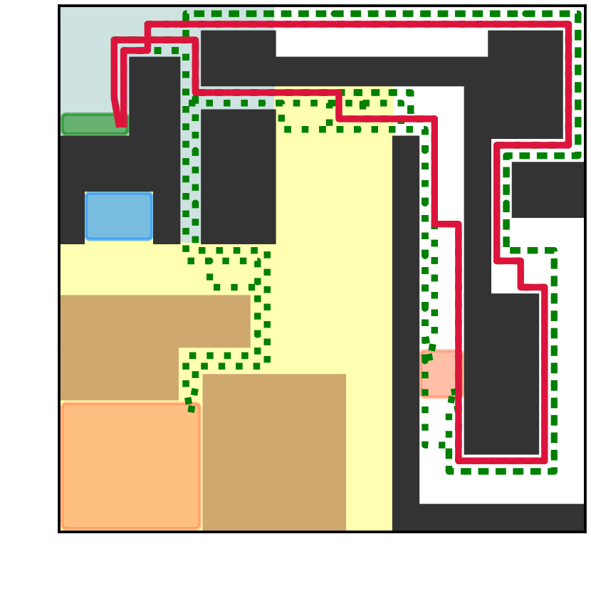
Suppose a Mars rover is tasked to collect scientifically interesting minerals from target sample sites (orange region in Fig. 5), designated based on past mission data [42]. Due to the limited number of sample tubes, it is required to go back and forth between the deposit location (green region) and the target site. Since the closer sampling region is in the sun, the rover must trade-off between low-time, high-radiation for efficient science data collection, or high-time, low-radiation to avoid long-term damage. Therefore, to protect itself while gaining sufficient amount of science, it must strike a balance between the two. Moreover, although the rover knows the qualitative information about the environment (e.g., where sand, base, washing station, etc. are located), it is still necessary to estimate online the time and radiation cost of collecting a sample. Informed by past mission data and scientific expertise, the user can tune an appropriate .
IV-A2 Simulation Setup
For the sake of simplicity, the rover can travel in cardinal directions, and may not move through obstacles (black). The task specification is given as
in English, “collect a sample, then deposit it, and, if sand is visited then wash before returning to base.” Each transition takes time (objective 1) measured in minutes, and transitions in the accumulate harmful radiation (objective 2) measured in micrograys. The true mean costs for transitions in each region are given as follows:
, and all other transitions have . Covariance values are omitted for brevity. The user informs the prior transition cost for all transitions to be . For the longevity of the rover, the user aims to endure a small amount of radiation and prefers that the mission is completed in roughly one and a half hours. To express this, the chosen preference distribution is
where is the - element of . Soon after deployment (instance 3), the planner only finds candidate plans that go through sand to collect the sample, and then must wash off, seen in Fig. 5(a). The robot quickly learns to avoid sand as washing takes very long and collects lots of radiation. The robot gradually discovers more optimal behavior seen by instance 25 in Fig. 5(b). In instance 35, seen in Fig. 5(c), the rover has roughly learned the true Pareto front, and elects to explore a less preferred, information rich trade-off. Finally, after 150 instances, seen in Fig. 5(d), the robot has obtained a fairly accurate estimate of the true Pareto front, and has converged to often selecting the most preferred trade-off.
IV-B Benchmarks
We evaluate the performance of our framework against the state-of-the-art in two benchmark problems. The goal is to assess in each instance: (i) how close the selected plan is to being Pareto optimal, and (ii) how well is represented by . Metric cumulative Pareto-regret directly evaluates (i). To properly evaluate (ii), we define Pareto-bias metric


for a true Pareto front and an estimate Pareto front as
| (22) |
where
is the Wasserstein-2 () distance. The first term in (22) quantifies the estimate Pareto front’s coverage of the true Pareto front, and the second term penalizes outlier/excess trade-offs in the estimate Pareto front. If each true Pareto point is exactly similar to an estimate Pareto point, and visa versa, then , otherwise .
We benchmarked our active inference (AIF) selection method against other state-of-the-art selection methods: uniform random selection (fair selection), TOPSIS [8] (objective preference), and linear scalarization, i.e. “weights” (subjective preference). Refer to Sec. V for further description of the compared methods.
IV-B1 Fixed Environment Case Study
Three grid world environments were designed to challenge the learning of different size Pareto fronts. All experiments were run for 300 instances, with a LCB confidence parameter , and Monte Carlo samples, selected via cross validation. See Appendix D for more details on the accuracy with respect to the choice of . Fig. 6 shows benchmarks against each environment. Generally, methods that accumulate less bias require learning more of the transition cost model via exploration, and hence accumulate more regret. When learning the small Pareto front, seen in Fig. 6(a), AIF performed better than both uniform and the biased methods (weights and TOPSIS) in terms of bias, with comparable regret to uniform. This is due to the advantageous information-gain-based exploration. When the number of Pareto points on the Pareto front increases, seen in Fig. 6(b), using small and no 222If the user only wants to specify a desired point in objective-space, they can make the preference distribution covariance very small (no variance) variance selects for only a portion of the true Pareto front, while the medium and large variance still envelope the entire Pareto front. With the smaller variance AIF methods, once a good estimate candidate is found, the first term of (III-C) dominates the selection, and thus abandons the less promising options that are beyond the variance. With an even larger Pareto front seen in Fig. 6(c), this effect is exacerbated. In this case, the no variance method sees a decrease in regret due to the heavy myopic bias after finding a candidate solution that agrees with the preference. Thus, from this experiment, we can observe that AIF methods start becoming very selective once the preferred region (which can be varied by the size of variance) on the Pareto front is discovered.
IV-B2 Random Environment Case Study
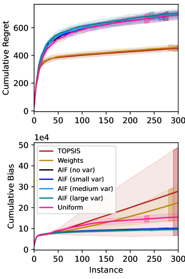
The behavior of our AIF selection method can vary widely across different scenarios depending on the diversity of the Pareto front relative to . Therefore, we illustrate the general behavior of our approach using randomized grid worlds. Each trial, a 2020 grid world robot model is generated with randomized proposition locations and true cost distribution parameters. The data was analyzed across 750 randomized trials.

Fig. 7 demonstrates the general trade-off between bias and regret. Note that the standard deviation in performance among trials is very large, since each randomly generated environment is diverse. When the variance of is large, active inference tends to perform similarly to random selection (Uniform) in terms of both regret and bias. With a moderate variance, active inference tends to have better regret and bias performance than other methods due to the intelligent information theoretic exploration when the estimate plans are uninformed. Uniform, AIF (large var), and AIF (medium var) stabilize in cumulative bias, meaning they effectively learn the entire Pareto front. The remaining methods converge to a non-constant slope cumulative bias, indicating that portions of the Pareto front have not been properly learned. From this experiment, we can observe that AIF methods outperform other state-of-the-art methods in terms of both cumulative regrets and biases as long as the size of variance is not too large.
Akin to other expected free energy approaches, the enhanced reasoning power comes at a computational cost compared to other methods [20, 31]. Uniform selection has complexity , weights has , and TOPSIS has [43]. We benchmarked the aforementioned random environment case studies with respect to both planning time and selection time per instance on a computer with AMD Ryzen 7 3800X 3.9 GHz 8-Core Processor. The average planning time is across 400 experiments with 100 instances each is ms (1-) with a median planning time of ms. The average AIF selection time (across all four preference distribution variances) is ms (1-) with a median selection time of ms. The compared selection procedures completed in less than ms.
Remark 1.
For larger-scale robotic models, the exact multi-objective graph search can be replaced with approximate multi-objective search, such as A∗pex [44], to admit a smaller (approximate) Pareto front in less time. Additionally, a clustering algorithm [45, 46] can further reduce the size of the Pareto front. We expect both adaptations to our framework to greatly enhance computation speed at the cost of Pareto-regret and bias performance, however we leave this to future work.
IV-C Hardware Experiment

To demonstrate the efficacy and diversity of application of our framework, we studied a complex dishwashing experiment using a robotic manipulator described in Fig. 1. The robot must repetitively load and unload the dishwasher with two items, a durable pitcher, and a fragile glass jar. The LTLf specification is
where
which can be interpreted as “put the pitcher and the jar in the dishwasher, then put the lid on, then for both the pitcher and jar, place on the drying rack, or dry the item and place it on the ground”. The performance of the robot is evaluated by the cumulative execution time (objective 1), as well as cumulative risk (objective 2) measured for a given action primitive,
| (23) |
where is the height of the jar above the ground. A sampling based motion planner (PRM∗ [47]) is used to realize motion action primitives, inducing unknown and random time and risk costs. Note that placing the jar on the drying rack is likely to have high risk, whereas manually drying the jar on the ground will likely take more time. We trained the transition cost model in simulation for instances, using a preference distribution of and , , , which selects for a high-time, low-risk alternative. The converged behavior is shown in Fig. 8. As can be seen, the robot correctly loads the dishwasher, then unloads the pitcher on the rack, and decides to manually dry the jar, all while not performing any sub-optimal/unnecessary actions. The video of the execution is included in the supplementary material and visually represents the applicability of our MORL framework to a variety of robotic models with complex tasks.
V Related Work
V-A Multi-Objective Reinforcement Learning
The goal of MORL is to maximize a multi-objective value or utility function [7]. MORL extends single-objective RL methods by selecting among Pareto-optimal candidate actions. One method of selection is casting valuations of candidate actions to a single-objective by scalarizing, in turn requiring a sound and interpretable utility function.
Scalarization of utility functions can be classified as subjective, scalarizing based on an exogenous user’s preferred trade-off [6], or non-subjective, scalarizing without external preferences [5, 8]. Linear scalarization is a standard subjective method that combines objectives objectives through a relative-importance weighted sum. On the contrary, non-subjective methods such as TOPSIS [8] and hyper-volume indicators [5] rely on Euclidian distance metrics in objective space. However, in many robotic applications where objectives have different units of measurement (e.g. time in seconds and energy in joules), these methods use the addition of quantities with different units, which is generally mathematically ad-hoc and lacks interpretation. Linear scalarization can potentially combat this issue by interpreting weights as reciprocal measures (e.g. second), at the cost of requiring a user to have a rigorous understanding of how to compare the importance of each objective and properly assign weights. Furthermore, re-interpreting units of measurement (e.g. seconds instead of milliseconds) alters Euclidian distance, which can dramatically alter the selected solution, when no fundamental aspects about the problem have changed. On the contrary, our method avoids this issue by only describing the scalarization through operations on probability density functions.
Many MORL methods do not distinguish between optimizing multi-objective value function and selecting the best action from the Pareto-optimal candidate actions [6, 7]. Instead, these methods scalarize using a monotonic utility function, which guarantees that an optimal (preferred) action with respect to the single-objective utility function must also be Pareto-optimal in objective space. The use of such a utility function effectively optimizes a single objective, which casts a complete order on the reward space and eliminates the need for explicit computation of the Pareto front beforehand. However, when a non-monotonic utility function is used, or the agent is concerned with learning the set of all optimal trade-off solutions [15], the Pareto front must be explicitly computed before selection, as seen in many MOMAB approaches. Our framework computes the Pareto front using a multi-objective task-planner.
MOMAB problems are concerned with minimizing Pareto-Regret [15], which uses -dominance to measure how “far” the chosen action is from being Pareto-optimal with respect to the true unknown reward distributions. Besides Pareto-regret, the MOMAB performance can also be evaluated by fairness, which quantifies how evenly Pareto-optimal actions were selected. Fairness is used to compare MOMAB selection by diversity in selection and learning of all actions on a possibly non-convex Pareto-front. To learn the entire Pareto front, work [15] extends the single-objective Upper Confidence Bound (UCB) algorithm [36] to multiple objectives, then rely on random selection among the Pareto front. While random selection effectively learns the entire Pareto front, it cannot account for or converge to a preferred trade-off. To address this shortcoming, our formulation of the high-level active inference decision making agent naturally balances this exploration vs. exploitation trade-off.
V-B Active Inference and Expected Free Energy
Active inference is an uncertainty-based sequential decision making scheme that applies the free energy principle (FEP) [48] to the behavioral norms of physical agents [19, 20, 21]. According to the FEP, agents intend to minimize the surprise (in our problem it is denoted as ) to maintain their homeostases. However, calculating the surprise directly requires to sum/integrate over all possible states/parameters in their internal generative models. When these quantities are continuous, depending on the prior and/or the likelihood function, the integral does not have a closed-form solution. Thus, some approximation methods are required to calculate the surprise.
One of the approaches is to employ variational Bayesian inference in statistical machine learning [40]. The core idea of this methodology is to introduce a proposal/surrogate distribution, which is easily modeled, and optimize the functional of this distribution to make it resemble a true intractable distribution. More specifically, in our problem, the following free-energy (FE, i.e. negative evidence lower bound) is minimized such that the Kullback-Leibler Divergence (KLD) between the proposal distribution and the true distribution approaches zero (Note that here we used the simplified notations seen in Appendices A and B).
| (24) |
As can be seen from this equation, since KLD is greater or equal to zero, FE is the upper bound of the surprise, i.e. minimizing FE leads to minimize the surprise.
Computation of FE is performed given an observed outcome observation , which is not known until the plan is executed. Hence, in active inference, the expected free energy (EFE) is instead minimized, and similar to FE, if the proposal and the true hidden posterior distributions match, the EFE term reduces to the following,
| (25) |
which is “expected” surprise. In summary, FE allows to make the surprise minimization tractable for continuous state/parameter systems, and EFE allows for the minimization FE without knowing the received observation a priori.
Additionally, as explained in (III-C), the EFE comprises of an utility term governed by a prior agent’s desired observation distribution, and an information gain term that evaluates how much a candidate action would reduce the uncertainty of hidden states/parameters. Hence, by minimizing EFE, the agents can naturally balance between two modes of behavior that are essential for autonomous decision making under uncertainty; exploitation (i.e. focusing on the current best action) and exploration (i.e. trying less executed actions). Furthermore, the degree of preference for either mode can be easily adjusted by varying the prior preference distribution. For instance, using a prior preference with a large variance will cause the agents to provide more priority to exploration, and vice versa. These characteristics are particularly useful when transparent agent behavior is desired [49]. Using active inference for selection marries the benefits of preferred versus fair selection described in Sec. V-A through localized information-theoretic exploration around the prior preference distribution. Additionally, specifying a preference distribution over desired trade-offs may be particularly intuitive, explainable, and even statistically informed with past data. Throughout this work, we study the benefits of using EFE in active inference for Pareto point selection in MORL with two statistical techniques when an intractable convolved NIW is used to represent the hidden parameters.
VI Conclusion and Future Work
In this work we study a systematic approach to learning Pareto-optimal behavior on an unknown multi-objective stochastic cost model. In particular we examine an active inference-based approach to multi-objective decision making and we examine the resulting behavior through robotic simulation and hardware experiments, and numerical benchmarks that compare against other state-of-the-art selection methods. Our approach marries the benefits of a user-provided preferred optimal trade-off with exploration required to learn portions of the entire Pareto front. We introduce a new Pareto-bias metric that, coupled with traditional Pareto-regret, elucidates the trade-off between accurately learning the diverse Pareto front versus quickly learning a single optimal trade-off. Notably, the balance between the aforementioned behaviors can be controlled via the user’s preference.
This work gives rise to a few future directions of research such as extension to stochastic transition models. Additionally, integrating cost-bounds for certain objectives by embedding a pruning procedure [14] into the multi-objective graph search algorithm is an interesting extension. Since the costs are not known a priori, we expect the Pareto cost upper confidence bound to be an effective choice of pruning constraint. We are also interested in generalizing the cost distribution to a Gaussian mixture to account for multi-modality. Other future directions may include convergence analysis and finite time regret analysis, for example, adapting the Upper Credible Limit algorithm [33] for Gaussian multi-armed bandits to the multi-objective setting.
References
- [1] Yang Gao and Steve Chien. Review on space robotics: toward top-level science through space exploration. Science Robotics, 2(7), 2017.
- [2] Jaeseok Kim, Anand Kumar Mishra, Raffaele Limosani, Marco Scafuro, Nino Cauli, Jose Santos-Victor, Barbara Mazzolai, and Filippo Cavallo. Control strategies for cleaning robots in domestic applications: A comprehensive review. International Journal of Advanced Robotic Systems, 16(4):1729881419857432, 2019.
- [3] Lydia E Kavraki, Petr Svestka, J-C Latombe, and Mark H Overmars. Probabilistic roadmaps for path planning in high-dimensional configuration spaces. IEEE transactions on Robotics and Automation, 12(4):566–580, 1996.
- [4] Sertac Karaman and Emilio Frazzoli. Sampling-based algorithms for optimal motion planning. The international journal of robotics research, 30(7):846–894, 2011.
- [5] Weijia Wang and Michèle Sebag. Multi-objective Monte-Carlo tree search. In Steven C. H. Hoi and Wray Buntine, editors, Proceedings of the Asian Conference on Machine Learning, volume 25 of Proceedings of Machine Learning Research, pages 507–522, Singapore Management University, Singapore, 04–06 Nov 2012. PMLR.
- [6] Axel Abels, Diederik M. Roijers, Tom Lenaerts, Ann Nowé, and Denis Steckelmacher. Dynamic weights in multi-objective deep reinforcement learning. In Kamalika Chaudhuri and Ruslan Salakhutdinov, editors, Proceedings of the 36th International Conference on Machine Learning, ICML 2019, 9-15 June 2019, Long Beach, California, USA, volume 97 of Proceedings of Machine Learning Research, pages 11–20. PMLR, 2019.
- [7] Conor F. Hayes, Roxana Rădulescu, Eugenio Bargiacchi, Johan Källström, Matthew Macfarlane, Mathieu Reymond, Timothy Verstraeten, Luisa M. Zintgraf, Richard Dazeley, Fredrik Heintz, Enda Howley, Athirai A. Irissappane, Patrick Mannion, Ann Nowé, Gabriel Ramos, Marcello Restelli, Peter Vamplew, and Diederik M. Roijers. A practical guide to multi-objective reinforcement learning and planning. Autonomous Agents and Multi-Agent Systems, 36(1), apr 2022.
- [8] Mohammad Mirzanejad, Morteza Ebrahimi, Peter Vamplew, and Hadi Veisi. An online scalarization multi-objective reinforcement learning algorithm: Topsis q-learning. The Knowledge Engineering Review, 37:e7, 2022.
- [9] Tuomas Haarnoja, Aurick Zhou, Kristian Hartikainen, George Tucker, Sehoon Ha, Jie Tan, Vikash Kumar, Henry Zhu, Abhishek Gupta, Pieter Abbeel, et al. Soft actor-critic algorithms and applications. arXiv preprint arXiv:1812.05905, 2018.
- [10] Saurabh Arora and Prashant Doshi. A survey of inverse reinforcement learning: Challenges, methods and progress. Artificial Intelligence, 297:103500, 2021.
- [11] Hadas Kress-Gazit, Morteza Lahijanian, and Vasumathi Raman. Synthesis for robots: Guarantees and feedback for robot behavior. Review of Control, Robotics, and Autonomous Systems, 1:211–236, May 2018.
- [12] Christel Baier and Joost-Pieter Katoen. Principles of Model Checking (Representation and Mind Series). The MIT Press, 2008.
- [13] Giuseppe De Giacomo and Moshe Y Vardi. Linear temporal logic and linear dynamic logic on finite traces. In IJCAI’13 Proceedings of the Twenty-Third international joint conference on Artificial Intelligence, pages 854–860. Association for Computing Machinery, 2013.
- [14] Peter Amorese and Morteza Lahijanian. Optimal cost-preference trade-off planning with multiple temporal tasks. In 2023 IEEE/RSJ International Conference on Intelligent Robots and Systems (IROS), pages 2071–2077, 2023.
- [15] Madalina M. Drugan and Ann Nowe. Designing multi-objective multi-armed bandits algorithms: A study. In The 2013 International Joint Conference on Neural Networks (IJCNN), pages 1–8, 2013.
- [16] Róbert Busa-Fekete, Balázs Szörényi, Paul Weng, and Shie Mannor. Multi-objective bandits: Optimizing the generalized gini index. In Proceedings of the 34th International Conference on Machine Learning - Volume 70, ICML’17, page 625–634. JMLR.org, 2017.
- [17] Eralp Turgay, Doruk Öner, and Cem Tekin. Multi-objective contextual bandit problem with similarity information. In Amos J. Storkey and Fernando Pérez-Cruz, editors, International Conference on Artificial Intelligence and Statistics, AISTATS 2018, 9-11 April 2018, Playa Blanca, Lanzarote, Canary Islands, Spain, volume 84 of Proceedings of Machine Learning Research, pages 1673–1681. PMLR, 2018.
- [18] Shiyin Lu, Guanghui Wang, Yao Hu, and Lijun Zhang. Multi-objective generalized linear bandits. IJCAI’19, page 3080–3086. AAAI Press, 2019.
- [19] Karl Friston, Francesco Rigoli, Dimitri Ognibene, Christoph Mathys, Thomas FitzGerald, and Giovanni Pezzulo. Active inference and epistemic value. Cognitive neuroscience, 02 2015.
- [20] Raphael Kaplan and Karl J. Friston. Planning and navigation as active inference. Biol. Cybern., 112(4):323–343, aug 2018.
- [21] Karl J Friston, Maxwell JD Ramstead, Alex B Kiefer, Alexander Tschantz, Christopher L Buckley, Mahault Albarracin, Riddhi J Pitliya, Conor Heins, Brennan Klein, Beren Millidge, Dalton AR Sakthivadivel, Toby St Clere Smithe, Magnus Koudahl, Safae Essafi Tremblay, Capm Petersen, Kaiser Fung, Jason G Fox, Steven Swanson, Dan Mapes, and Gabriel René. Designing ecosystems of intelligence from first principles. Collective Intelligence, 3(1):26339137231222481, 2024.
- [22] Shohei Wakayama and Nisar Ahmed. Active inference for autonomous decision-making with contextual multi-armed bandits. In 2023 IEEE International Conference on Robotics and Automation (ICRA), pages 7916–7922, 2023.
- [23] Marius Kloetzer and Calin Belta. A fully automated framework for control of linear systems from temporal logic specifications. IEEE Transactions on Automatic Control, 53(1):287–297, 2008.
- [24] Georgios E Fainekos, Hadas Kress-Gazit, and George J Pappas. Temporal logic motion planning for mobile robots. In Proceedings of the 2005 IEEE International Conference on Robotics and Automation, pages 2020–2025. IEEE, 2005.
- [25] Shuo Yang, Xiang Yin, Shaoyuan Li, and Majid Zamani. Secure-by-construction optimal path planning for linear temporal logic tasks. In 2020 59th IEEE Conference on Decision and Control (CDC), pages 4460–4466. IEEE, 2020.
- [26] Georgios E Fainekos, Hadas Kress-Gazit, and George J Pappas. Hybrid controllers for path planning: A temporal logic approach. In Proceedings of the 44th IEEE Conference on Decision and Control, pages 4885–4890. IEEE, 2005.
- [27] Keliang He, Morteza Lahijanian, Lydia E Kavraki, and Moshe Y Vardi. Towards manipulation planning with temporal logic specifications. In 2015 IEEE international conference on robotics and automation (ICRA), pages 346–352. IEEE, 2015.
- [28] Keliang He, Morteza Lahijanian, E Kavraki, Lydia, and Y Vardi, Moshe. Automated abstraction of manipulation domains for cost-based reactive synthesis. IEEE Robotics and Automation Letters, 4(2):285–292, Apr. 2019.
- [29] Pablo Lanillos, Cristian Meo, Corrado Pezzato, Ajith Anil Meera, Mohamed Baioumy, Wataru Ohata, Alexander Tschantz, Beren Millidge, Martijn Wisse, Christopher L. Buckley, and Jun Tani. Active inference in robotics and artificial agents: Survey and challenges. CoRR, abs/2112.01871, 2021.
- [30] Thomas M. Cover and Joy A. Thomas. Elements of Information Theory (Wiley Series in Telecommunications and Signal Processing). Wiley-Interscience, USA, 2006.
- [31] Ryan Smith, Karl J. Friston, and Christopher J. Whyte. A step-by-step tutorial on active inference and its application to empirical data. Journal of Mathematical Psychology, 107:102632, 2022.
- [32] Kevin P. Murphy. Conjugate bayesian analysis of the gaussian distribution. 2007.
- [33] Paul B Reverdy, Vaibhav Srivastava, and Naomi Ehrich Leonard. Modeling human decision making in generalized gaussian multiarmed bandits. Proceedings of the IEEE, 102(4):544–571, 2014.
- [34] Yen-Chi Chen. A tutorial on kernel density estimation and recent advances. Biostatistics & Epidemiology, 1(1):161–187, 2017.
- [35] Lawrence Mandow and José Luis Pérez De La Cruz. Multiobjective a* search with consistent heuristics. Journal of the ACM (JACM), 57(5):1–25, 2008.
- [36] Peter Auer, Nicolò Cesa-Bianchi, and Paul Fischer. Finite-time analysis of the multiarmed bandit problem. Mach. Learn., 47(2–3):235–256, may 2002.
- [37] David M Blei, Alp Kucukelbir, and Jon D McAuliffe. Variational inference: A review for statisticians. Journal of the American statistical Association, 112(518):859–877, 2017.
- [38] Horia Mania, Stephen Tu, and Benjamin Recht. Certainty equivalence is efficient for linear quadratic control. Advances in Neural Information Processing Systems, 32, 2019.
- [39] Sang Gyu Kwak and Jong Hae Kim. Central limit theorem: the cornerstone of modern statistics. Korean journal of anesthesiology, 70(2):144–156, 2017.
- [40] Christopher M. Bishop. Pattern Recognition and Machine Learning (Information Science and Statistics). Springer-Verlag, Berlin, Heidelberg, 2006.
- [41] William L Dunn and J Kenneth Shultis. Exploring monte carlo methods. Elsevier, 2022.
- [42] Kenneth A Farley, Kenneth H Williford, Kathryn M Stack, Rohit Bhartia, Al Chen, Manuel de la Torre, Kevin Hand, Yulia Goreva, Christopher DK Herd, Ricardo Hueso, et al. Mars 2020 mission overview. Space Science Reviews, 216:1–41, 2020.
- [43] Hamdani Hamdani and Retantyo Wardoyo. The complexity calculation for group decision making using topsis algorithm. In AIP conference proceedings, volume 1755. AIP Publishing, 2016.
- [44] Han Zhang, Oren Salzman, TK Satish Kumar, Ariel Felner, Carlos Hernández Ulloa, and Sven Koenig. A* pex: Efficient approximate multi-objective search on graphs. In Proceedings of the International Conference on Automated Planning and Scheduling, volume 32, pages 394–403, 2022.
- [45] Enrico Zio and Roberta Bazzo. A clustering procedure for reducing the number of representative solutions in the pareto front of multiobjective optimization problems. European Journal of Operational Research, 210(3):624–634, 2011.
- [46] Lilian Astrid Bejarano, Helbert Eduardo Espitia, and Carlos Enrique Montenegro. Clustering analysis for the pareto optimal front in multi-objective optimization. Computation, 10(3):37, 2022.
- [47] SM LaValle. Planning Algorithms, volume 2. 2006.
- [48] K. Friston. The free-energy principle: A unified brain theory? Nature Reviews Neuroscience, 11(2):127–138, 2010.
- [49] Shohei Wakayama and Nisar Ahmed. Observation-augmented contextual multi-armed bandits for robotic exploration with uncertain semantic data. arXiv, (2312.12583), 2023.
- [50] Robert A. Stine. Explaining normal quantile-quantile plots through animation: The water-filling analogy. The American Statistician, 71(2):145–147, 2017.
- [51] Zafeirios Fountas, Noor Sajid, Pedro Mediano, and Karl Friston. Deep active inference agents using monte-carlo methods. Advances in neural information processing systems, 33:11662–11675, 2020.
- [52] Alexander Tschantz, Manuel Baltieri, Anil. K. Seth, and Christopher L. Buckley. Scaling active inference. In 2020 International Joint Conference on Neural Networks (IJCNN), pages 1–8, 2020.
- [53] Domenico Maisto, Francesco Gregoretti, Karl J. Friston, and Giovanni Pezzulo. Active tree search in large pomdps. ArXiv, abs/2103.13860, 2021.
Appendix A Derivation of EFE for the Pareto Point Selection
As mentioned in Sec. III-C, marginalizing the joint distribution is analytically intractable. Therefore, its bound, i.e. free energy, is minimized instead. Yet, the outcomes cannot be observed until a plan is actually executed, so the agent ends up minimizing EFE. Hereafter, for the sake of simplicity, we denote as , as , and as .
| (26) |
where is the prior preference for outcomes and is the proposal distribution for and given a plan . Eq. (A) can be decomposed into three parts as follows.
| (27) |
| (28) |
| (29) |
By combining these parts, (III-C) is finally derived.
Appendix B Approximation for the First Term of (III-C)
In order to approximate the first term of (III-C), can be at first simplified as follows.
| (30) |
where . Recall, the certainty equivalence approximation for the predicted observation distribution is a MVN distribution . By substituting this result into (III-C), the first term of (III-C) can be further transformed as
| (31) |
Since is expanded as , the second term of (31) is turned to
| (32) | ||||
| (33) | ||||
| (34) |
Finally, (32) can be reduced to
where . Also, (33) is simply
and (34) can be reduced to
Appendix C Empirical Analysis of Error Introduced via NIW-MVN Substitution
To evaluate the choice of approximate posterior described in Sec. III-C3, we numerically demonstrated the efficacy of substituting intractable convolved NIW distributions (denoted ) with convolutions of MVN (denoted ). Additionally, since the same substitution technique is used for choosing the prior proposal distribution in (15), this analysis also yields insight into the quality of the variational upper bound.


Following (13) and (14), and must have the same mean and variance, therefore, it suffices to analyze the normality of Monte Carlo samples of for determining how well approximates . This analysis is done using a Quantile-Quantile (Q-Q) plot [50]. The procedure for generating Monte Carlo samples used in the Q-Q plot is outlined as follows:
-
1.
Generate number of samples of from each respective NIW . For high fidelity, we used samples.
-
2.
Sum each respective sample to get samples of , (empirically representing samples from ),
-
3.
Perform a whitening transform to all such that the such that the mean is zero and the covariance is normalized and uncorrelated,
-
4.
Produce a Q-Q plot to assess the normality of the whitened empirical distribution.
The resulting Q-Q plots are shown in Fig. 9. The distributions of the mean parameters (Fig. 9(a), top row) are generally well approximated by . For short plans , the covariance parameter distributions differ from slightly (Fig. 9(a), bottom left), however, due to the Central Limit Theorem (CLT), they converge to normal as the length of the plan increases (Fig. 9(a), bottom right). Similarly, as more data is supplied to each state-action pair, the distribution becomes more normal due to the Inverse Wishart distribution being less right-skewed (Fig. 9(b), bottom left to bottom right). Therefore, the MVN replacement approximation introduces less error as the scenarios become more complex, and more data is collected.
Appendix D Empirical Analysis of Error Introduced via Monte Carlo Sampling
Fig. 10 shows the percent error introduced via sampling. Note that was used for the experiments and benchmarks shown in the manuscript as well as the computation time benchmarks. Although the specific sampling procedure is slightly different, there are multiple studies using the Monte Carlo sampling to evaluate the EFE [51, 52, 53].