Quiescent black hole X-ray binaries as multi-messenger sources

Galactic cosmic rays (CRs) are of unknown origin, even though they have traditionally been connected to supernovae due to energetic arguments. In the last decades, Galactic black holes in X-ray binaries (BHXBs) have been proposed as candidate sources of CRs revising the CR paradigm. BHXBs launch two relativistic jets during outbursts, but recent observations suggest that such jets may be launched even during quiescence. A0620–00 is such a well-studied object that shows hints of jet emission. In this work, we study the simultaneous radio-to-X-ray spectrum detected from this source while in quiescence to better constrain the jet dynamics. Given that the majority of BHXBs spend their lifetime in quiescence (qBHXBs), we use the jet dynamics of A0620–00 to study a population of $10^{5}$ such sources distributed throughout the Galactic disc, and a further $10^{4}$ located in the Boxy Bulge around the Galactic centre. While the contribution to the CR spectrum is suppressed, we find that the cumulative intrinsic emission of qBHXBs from both the Boxy Bulge and the Galactic disc adds to the diffuse emission that various facilities detect from radio to TeV $\gamma$ rays. We examine the contribution of qBHXBs to the Galactic diffuse emission and investigate the possibility of SKA, INTEGRAL and CTAO to detect individual sources in the future. Finally, we compare the predicted neutrino flux to the recently presented Galactic diffuse neutrino emission by IceCube.

1 Introduction

Cosmic rays (CRs) are charged particles of extraterrestrial origin. Despite decades of research, we still lack a full understanding of the CR sources and the physical mechanism behind their acceleration. When CRs accelerate, they reach high energies to allow the emission of $\gamma$ rays. Leptonic CRs on one hand can upscatter background radiation to $\gamma$ rays, and hadronic CRs on the other hand, may interact inelastically with background photons and/or gas to produce secondary particles, such as $\gamma$ rays and neutrinos (Mannheim & Schlickeiser, 1994).

Traditionally, the explosive deaths of massive stars have been considered Galactic CR sources (Baade & Zwicky, 1934; Ginzburg & Syrovatskii, 1964; Blasi, 2013). Numerous works have recently suggested stellar mass black holes (BHs) in X-ray binaries (XRBs – BHXBs, henceforth) as promising candidates for CR sources (Romero et al., 2003; Fender et al., 2005; Bednarek et al., 2005; Torres et al., 2005; Reynoso et al., 2008; Cooper et al., 2020; Carulli et al., 2021). In particular, stellar-mass BHs in XRBs accrete mass from the companion star and when they outgo into outburst they launch two relativistic jets (Mirabel & Rodriguez, 1994; Corbel et al., 2000, 2012; Fender, 2001; Corbel & Fender, 2002; Fender et al., 2004, 2009; McClintock et al., 2006). These jets can accelerate particles to high energies, leaving their imprint in the radio-to-$\gamma$-ray regime, such as the cases of Cygnus X–1 (Gallo et al., 2005; Zanin et al., 2016), Cygnus X–3 (Miller-Jones et al., 2004; Tavani et al., 2009) and more recently SS433 that was detected even in the PeV (Abeysekara et al., 2018; Safi-Harb et al., 2022).

BHXBs are observed to launch jets during outbursts, mainly during the so-called hard X-ray spectral state (McClintock et al., 2006) but sometimes also during the soft state (see, i.e. the case of Cygnus X–3, Koljonen et al. 2010; Cangemi et al. 2021). Recent simultaneous radio-to-X-ray observations show evidence of a flat radio spectrum along with a hard X-ray spectrum from several BHXBs in quiescence (qBHXBs; Gallo et al. 2007; Maitra et al. 2009; Plotkin et al. 2013, 2014, 2017; Gallo et al. 2014; Connors et al. 2016; Dinçer et al. 2017; dePolo et al. 2022). These spectral features hint at the existence of a pair of relativistic jets that however carry significantly less power compared to those during the outburst.

To better capture jet physics and understand the particle acceleration along the jets, several models have been suggested in the past (Tavecchio et al., 1998; Mastichiadis & Kirk, 2002; Marscher et al., 2008; Tramacere et al., 2009). Based on the nominal work of Blandford & Königl (1979), a multi-zone jet prescription is capable of reproducing the multi-wavelength spectral emission we detect from such sources, as well as describing the jet morphology that numerous sources demonstrate (see e.g. Janssen et al., 2021). In this work, we use the multi-zone jet model as initially sketched by Markoff et al. (2001) and Markoff et al. (2005), and further developed by Lucchini et al. (2022) for a purely leptonic non-thermal emission, and Kantzas et al. (2021) expanding to lepto-hadronic radiative processes. More precisely, we use and compare two different jet scenarios. In the first one, we expand the jet dynamics of Lucchini et al. (2022) to include the hadronic interactions as described in Kantzas et al. (2021) and we refer to this model as BHJet. The second scenario, is the mass-loading case of Kantzas et al. (2023) that was developed to address the proton-power problem, namely what is the origin of the energy excess that is used by protons to accelerate to high energies (Böttcher et al., 2013; Liodakis & Petropoulou, 2020), and we refer to this model as MLJet.

Despite being faint and many times failing to exceed the observability threshold, there are still a few qBHXBs detected. A0620–00, for instance, demonstrates a flat radio spectrum and recent modelling of the X-ray spectrum does not rule out some significant jet contribution (Gallo et al., 2007; Connors et al., 2016; Dinçer et al., 2017; dePolo et al., 2022). Such broadband coverage allows for more robust constraints of the jets’ contribution to the electromagnetic spectrum to better understand their dynamical properties. Based on the findings of the multi-wavelength spectral fitting of A0620–00, we investigate the possible contribution of the entire population of qBHXBs to the CR spectrum detected on Earth because tens to hundreds of thousands of such sources may reside in the Milky Way (see e.g. Olejak et al. 2020 and references below).

While, as we will show, the contribution to the Galactic CR spectrum is negligible, a further, indirect, indication for CR acceleration is the total contribution of qBHXB jets to the observed diffuse emission in multiple frequencies. For example, the X-ray background, especially in the 1-100 keV energy range, is relatively well studied: The bulk of this emission, about 90% should mainly originate in cataclysmic events, while the remaining 10% can be produced by unresolved sources (Perez et al., 2019). Likewise, for the more energetic MeV X-ray diffuse background, some unresolved Galactic sources are required to explain the entire spectrum. Recently, pulsars were suggested as promising MeV emitter but due to lack of radio counterpart, qBHXBs cannot be ruled out yet (Berteaud et al., 2022, 2024). At higher energies, in the GeV and TeV bands, the picture is similarly fuzzy. In particular, the diffuse GeV background (Ackermann et al., 2012), especially towards the Galactic bulge, may also be due to dark matter annihilation and/or decay that complicates the search for the CR accelerators even further (Dodelson et al., 2008; Calore et al., 2015). Similarly, Galactic sources that emit at TeV energies and beyond are among the most powerful Galactic CR accelerators, probably sourcing the diffuse emission recently measured by LHAASO (Cao et al., 2023) and Tibet AS-$\gamma$ (Amenomori et al., 2021). In this work, we also examine the possible contribution of qBHXBs to the diffuse multi-wavelength cosmic backgrounds.

In Section 2, we describe the jet model we use in this work, and we apply it to A0620–00 in Section 3. We investigate the possible contribution of the entire population of qBHXBs to the diffuse emission in Section 4, and finally, we discuss the results of this work in Section 5 and conclude in Section 6.

2 Jet emission

2.1 BHJet

The jets launched by BHXBs share similar physical properties as the AGN jets but on much smaller scales (Merloni et al., 2003; Falcke et al., 2004). In this work, we further develop the multi-zone jet model that describes the flat to inverted radio spectra observed by BHXBs (see e.g. Russell & Shahbaz, 2014) and was initially presented in Falcke & Biermann (1994) and Markoff et al. (2001, 2003, 2005). The most recent and user-friendly version of this model, referred to as BHJet, is thoroughly described in Lucchini et al. (2022) and can be found in an online repository.

BHJet solves the transport equation of a mixed population of thermal and non-thermal electrons along the jet axis and estimates synchrotron and inverse Compton scattering (IC) emissions. Such a complex but still physically motivated jet prescription can prove useful in understanding jet kinematics of not only small-scale jets (see e.g. Maitra et al. 2009; Plotkin et al. 2011, 2014; Markoff et al. 2015; Connors et al. 2019; Lucchini et al. 2021; Kantzas et al. 2021, 2022), but also large scale AGN jets (see e.g. Lucchini et al. 2018, 2019). In either case, two fundamental aspects succeed to well explaining the electromagnetic constraints. Firstly, a Poynting flux-dominated, thermal but still relativistic jet base explains well the infrared (IR) observations and especially those that hint at jet contribution (see e.g. Gallo et al. 2007; Gandhi et al. 2011 and references above). Such a jet base is described by its initial radius $r_{0}$, the injected power $P_{\rm jet}$, the temperature of the relativistic electrons $T_{e}$, and the equipartition arguments. $r_{0}$, $P_{\rm jet}$ and $T_{e}$ are free parameters and for simplicity, we assume that the plasma $\beta$, defined as the energy density of the gas over the energy density of the magnetic field, is equal to 0.02 (see Lucchini et al. 2022 for a detailed explanation). Finally, the exact composition of the jet is not fully understood, but a simple assumption of an equal number of electrons and protons is broadly accepted.

Far beyond the jet base and at some distance that usually reaches the tens to thousands of gravitational radii a fraction of the thermal electrons start to accelerate to a non-thermal power law in energy due to some particle acceleration mechanism for which we remain agnostic. This region that we call ‘particle acceleration region’ is located at some distance $z_{\rm diss}$ and is where the jet energy is further dissipated into bulk velocity, the magnetisation (defined as $\sigma=B^{2}/4\pi\rho c^{2}$, where $B$ is the magnetic field strength and $\rho$ mass density of the jet segment), the particles. This location is also the transition between an optically thin to an thick jet plasma that explains the spectral break that is usually detected in the IR band of the spectrum (see, e.g. Gandhi et al. 2011; Russell et al. 2014). Since the particle acceleration region is tightly connected to the jet base, its dynamical properties such as the radius and the strength of the magnetic field depend on its distance from the BH, which is a free parameter.

As already mentioned, we remain agnostic about the particle acceleration mechanism, which can however significantly alter the observational imprints. To better investigate the effect of such a particle acceleration, but also without increasing the number of free parameters, we assume that the minimum electron energy of the power law is the peak of the thermal distribution at $T_{e}$, and the index $p$ remains a free parameter. We calculate the maximum energy of the non-thermal electrons by equating the characteristic timescales of the acceleration and the radiative losses. For an efficient particle acceleration and the case of BHXBs, the non-thermal electrons reach energies of the order of tens of GeV. Such energetic electrons in the strong magnetic fields of the jets can produce a hard synchrotron spectrum that shines up to X rays. Further upscattering of these X rays by the non-thermal electrons can explain the GeV $\gamma$ rays detected by such sources (Tavani et al., 2009; Zanin et al., 2016).

Such a purely leptonic jet model such as the one we discussed so far can sufficiently explain the overall electromagnetic emission detected by BHXB and AGN jets but cannot treat the acceleration of hadronic particles that is likely to occur inside such sources, due to the correlation to astrophysical neutrinos (Keivani et al., 2018). To better investigate the hadronic acceleration and the contribution of flaring BHXBs to the CR spectrum, we developed a lepto-hadronic jet model in Kantzas et al. (2021). The jet dynamics assumed in that work was a pressure-driven jet that may even be particle-dominated because the particle energy density dominates the Poynting flux. For the first time, to allow for a Poynting flux-dominated jet that includes the inelastic hadronic processes, we combine the jet dynamics of BHJet with the hadronic processes discussed in Kantzas et al. (2021). More specifically, similar to the non-thermal electrons, we assume that the protons are initially cold. At the dissipation region, a fraction of protons populates a power law in energy from some minimum energy of 1  GeV up to some maximum energy that is self-consistently calculated per jet segment, following a similar prescription as the Hillas criterion (Hillas, 1984; Jokipii, 1987). The power-law index remains a free parameter that is the same for both electrons and protons for simplicity. The non-thermal protons of each jet segment interact inelastically with the cold protons of the jet flow, the radiation of this specific jet segment, and other photon/gas fields such as the companion star radiation field and its stellar wind. The proton-proton (pp) and photohadronic (p$\gamma$) interactions lead to the formation of distributions of charged and neutral pions that eventually decay into $\gamma$ rays, secondary electrons and neutrinos (Mannheim, 1993; Mannheim & Schlickeiser, 1994; Rachen & Biermann, 1993; Rachen & Mészáros, 1998; Mücke et al., 2003). These interactions, due to complexity, require Monte Carlo simulations to properly produce the secondary populations. Such time and source-consuming processes though would not allow for a fast comparison with observational data, we hence choose to use the semi-analytical formulae of Kelner et al. (2006) for pp, and Kelner & Aharonian (2008) for p$\gamma$, respectively.

2.2 MLJet

Recent numerical magnetohydrodynamic simulations in the general relativity regime (GRMHD) show that not only a Poynting flux-dominated jet is a natural output of the Blandford & Znajek (1977) and Blandford & Payne (1982) launching mechanisms, but also a significant fraction of the energy is dissipated to particles. Chatterjee et al. (2019) for instance, performed one of the highest 2D resolution GRMHD simulations to show that instabilities in the interface between the jet edge and the wind of the accretion disc allow for eddies that transport matter from the wind to the jet. Hybrid GRMHD and particle-in-cell simulations of such setups prove that particle acceleration indeed happens and particles gain non-thermal energies (Sironi et al., 2021).

In Kantzas et al. (2023) we capture the macroscopic picture of such a mass-loading scenario where we adopt the jet dynamics from the GRMHD simulations and combine it with the lepto-hadronic processes. We refer to this scenario as MLJet. More precisely, we parametrise the profiles along the jet axis of the bulk velocity, the magnetisation, and the specific enthalpy, which is an estimate of the excess energy that is converted to non-thermal protons. The initial setup is once more driven by the physics of the jet base and the jet region, where the mass-loading starts to become important (we adopt the same parameter as BHJet, namely $z_{\rm diss}$). The mass loading initiates at a distance $z_{\rm diss}$ from the BH and dies off at $\sim 10\,z_{\rm diss}$ (see discussion in Chatterjee et al. 2019 and Kantzas et al. (2023)). A further vital aspect is the initial magnetisation at the jet base because this amount of energy will lead not only to the bulk jet acceleration but also will allow for more abundant hadronic counterparts. We adopt a relatively mediocre value of $\sigma=10$ and a bulk Lorentz factor after reaching a maximum value of 3 at $z_{\rm diss}$. Finally, a further important macroscopic quantity is the jet composition. In MLJet, we assume that the jet is launched lepton-dominated with the ratio of electrons to protons to be a free parameter $\eta=n_{e}/n_{p}$, where $n_{e}$ is the number density of pairs of electrons, and $n_{p}$ is the number density of protons. At the maximum of the mass-loading, we assume an equal number of electrons and protons to entrain the jets, modifying their dynamics. This assumption ensures that the jet remains charge-neutral despite the mass loading. All the free parameters used in this work, and in particular for the case of A0620–00, are tabulated in Table 1.

3 Studying the prototypical case of A0620–00

A0620–00 is a typical qBHXB located at a distance of $1.06\pm 0.12$ kpc (Cantrell et al., 2010). The mass of the BH is estimated to be $6.61\pm 0.25\,\rm M_{\odot}$ and the inclination of the system is $51\pm 1^{\circ}$ (Cantrell et al., 2010). We use the multi-wavelength observations of Dinçer et al. (2017) that cover the entire electromagnetic spectrum from radio (VLA), to optical/near-infrared (SMARTS telescope) and X rays with Chandra. We use the observation performed on 2013 December 9th, and we plot the output in Fig. 1. In this figure, in particular, we plot the best fit of BHJet to the observational data in the upper panel, and the best fit of MLJet in the lower panel. To find the best fit for either jet model, we use the Interactive Spectral Interpretation System (ISIS; Houck & Denicola 2000) to forward fold the model into X-ray detector space. We use the EMCEE function to explore the parameter space using a Markov chain Monte Carlo method (Foreman-Mackey et al. 2013. We perform $10^{4}$ loops with 20 initial walkers per free parameter, and we reject the first 50% of the runs until the method approaches good statistical significance. In Table 1, we list the free parameters of the two models, along with the results of the best fit and the $1\,\sigma$ uncertainties. In Fig. 1, we indicate the total flux density accounting for absorption, as well as all the individual components from the jet base, the jet, and the companion star, as shown in the legend. The sub-panel in each panel shows the residuals of the model.

In Fig. 2, we show the extended energy spectrum including not only the radio-to-X-ray data but also the sensitivity curves of three instruments in the high-energy regime. We use, in particular, the sensitivity curve of INTEGRAL/SPI, the Fermi/LAT sensitivity, and the predicted CTA sensitivity for the South site. The upper panel is for the case of BHJet, and the lower panel is for the case of MLJet. The contribution from the secondary particles and the individual components are as shown in the legend.

Parameter	Model		Description
	BHJet	MLJet
$P_{\rm jet}/\rm L_{Edd}$	$2.86\pm 0.03\times 10^{-5}$	$7_{-4}^{+30}\times 10^{-6}$	Injected power at the jet base
$r_{0}/r_{g}$	$6.3_{-0.5}^{+0.1}$	$11_{-4}^{+9}$	Jet-base radius
$z_{\rm diss}/r_{g}$	$73\pm 1$	$4\pm 1$	Particle acceleration region
$k_{B}T_{e}/\rm keV$	$1800_{-10}^{+40}$	$2600_{-100}^{+1700}$	Jet-base electron temperature
$p$	$2.070_{-0.001}^{+0.003}$	$2.2_{-0.1}^{+0.2}$	Power-law slope of non-thermal particles
$\eta_{e}$	1 (fixed)	$190_{-180}^{+240}$	pair-to-electron/proton ratio

Table 1: The free (fitted) parameters of the multi-wavelength spectral modelling fit to A0620–00.

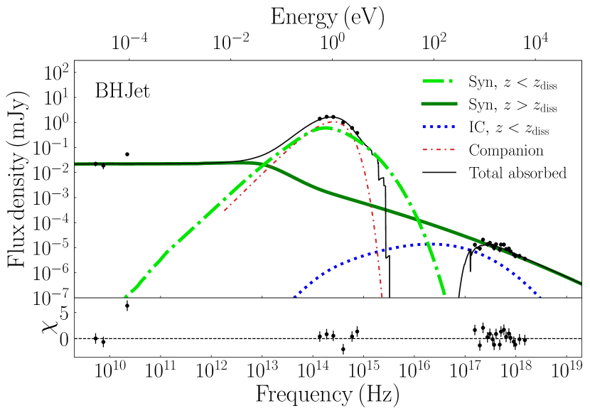
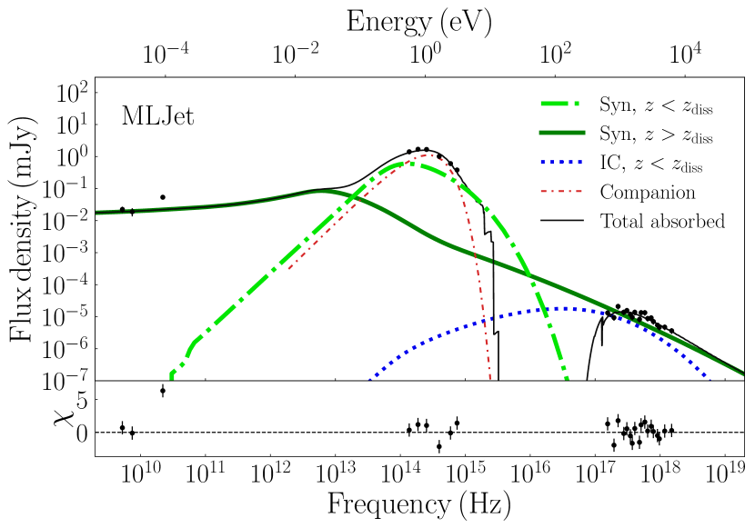
Figure 1: The best fit with residuals of the multi-wavelength flux density of the 2013 observations of A0620–00 from Dinçer et al. (2017). In the upper panel, we show the result for the case of BHJet, and in the lower panel, we show the case of MLJet. The solid black line shows the total absorbed emission, and the individual components are explained in the legend.

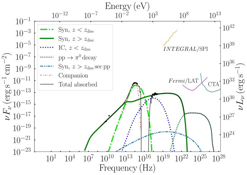
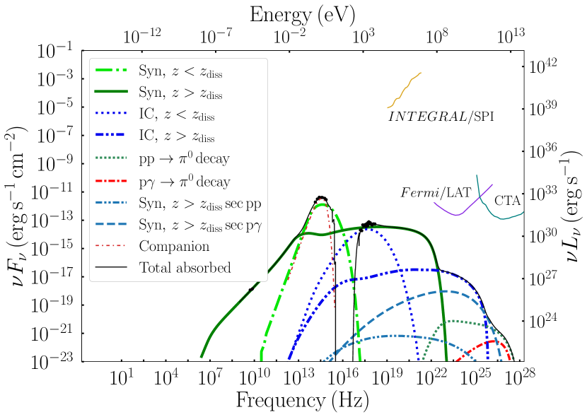
Figure 2: The multi-wavelength spectrum of A0620–00 for the case of the BHJet model in the upper panel and for the case of the MLJet model in the lower panel. The solid black line shows the total emitted spectrum, and the individual components are explained in the legends. The radio-to-X-ray data are the same as in Fig. 1. We include the INTEGRAL/SPI, Fermi/LAT, and CTA point source sensitivities for comparison.

4 The multi-wavelength emission of qBHXBs

4.1 Population model

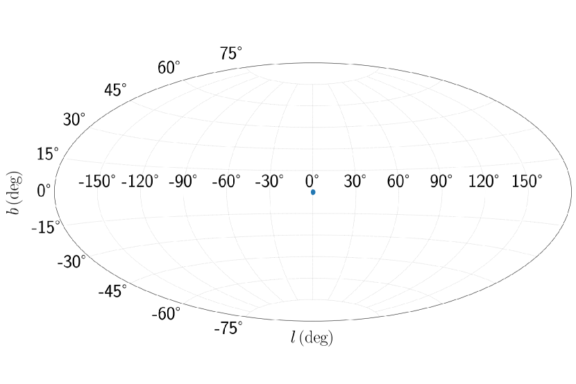
(a) $10^{3}$ qBHXBs located at the GC.

(b) The distribution of distances of the GC qBHXBs.

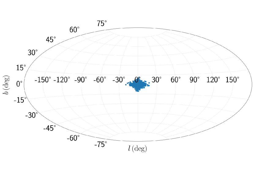
(c) $10^{4}$ qBHXBs located at the Boxy Bulge.

(d) The distribution of distances of the Boxy Bulge qBHXBs.

(e) $1.2\times 10^{5}$ qBHXBs located at the Galactic disc.

(f) The distribution of distances of the disc qBHXBs.

Figure 3: The positions of one random realisation of qBHXBs in the sky (left) in Galactic coordinates and the histogram of their distances (right). From top to bottom, we plot the sources at the GC, the Boxy Bulge, and the Galactic disc.

(a) $10^{4}$ qBHXBs located in the Boxy Bulge.

(b) $1.2\times 10^{5}$ qBHXBs located in the Galactic disc.

Figure 4: The histogram of the masses of the BH of the qBHXBs. The grey-shaded region is adopted from Olejak et al. (2020), from which we derive a Gaussian kernel shown by the solid line. The orange-shaded histogram corresponds to $10^{4}$ Boxy Bulge qBHXBs (left panel) and $1.2\times 10^{5}$ disc qBHXBs (right panel) used in this work.

The simultaneous radio to X ray observations of binary systems have led to the identification of around 50 BHXBs (Corral-Santana et al., 2016; Tetarenko et al., 2016b). The duty cycle of these sources is approximately 10 %, namely they spend most of their lifetime in quiescence. Following the work of Olejak et al. (2020) we extract information on a recent population synthesis analysis. More precisely, we study separately three different regions of the Milky Way; a Lorimer-like population of qBHXB in the Galactic disc (Lorimer et al., 2006), a further population in the Boxy Bugle, and a third distribution up to a few tens of pc around the Galactic centre (GC). As the absolute size of each population, we adopt the following numbers: $10^{3}$ sources in the GC, $10^{4}$ in the Boxy Bulge, and an upper limit of $1.2\times 10^{5}$ sources in the disc (Olejak et al. 2020 and see discussion below). We draw random values in a 3D grid to place the sources in the three different Galactic regions, namely, we adopt a Gaussian distribution for the radial distances of the GC sources with a mean value of 2 pc and a standard deviation of 20 pc (Mori et al., 2021). For the Boxy Bulge we follow the formula of Cao et al. (2013) and for the disc sources we adopt the Lorimer distribution of Lorimer et al. (2006). We assume that the Galactic disc is a 2D structure of a radius of 20 kpc and height of 2 kpc above and below the Galactic plane, and the location of the solar system at 8.3 kpc from the GC. In Fig. 3, we show the sky map and the distances of the sources of each individual population with the GC on top, the Boxy Bulge in the middle, and the Lorimer-like in the lower panels. On the left panels, we show the sky maps in Galactic coordinates, and on the right, we plot the histograms of the distances of the produced qBHXBs from the Sun.

Besides the spatial positions, we also need to model the BH mass distribution. Olejak et al. (2020) present the distribution of the mass of the BH in binaries for the Galactic disc and the Galactic halo. In Fig. 4, we plot the histogram based on the supplementary material of Olejak et al. (2020), for which we find a Gaussian kernel to use as probability function distribution (PDF). From this calculated PDF, we extract $10^{4}$ and $1.2\times 10^{5}$ random values of the mass of the BH for the Boxy Bulge and the Lorimer-like distribution, respectively. We plot the extracted random values as an orange-shaded histogram on top of the resulting distribution of Olejak et al. (2020).

A further impactful parameter of the qBHXBs is the viewing angle, namely the angle between the jet axis and the line of sight. Due to the lack of robust constraints, we use a uniform PDF between $1^{\circ}$ and $90^{\circ}$ to evaluate the viewing angle of each qBHXB.

For each unique source, we assume a set of parameters of a mass of the BH, a viewing angle, and a distance. Assuming that all qBHXBs have similar behaviour to A0620–00, we use these three quantities, to rescale the emitted spectrum.

Figure 5: The contribution of the prompt emission of the Galactic qBHXBs to the NuSTAR diffuse emission for $1^{\circ}\leq(l,b)\leq 3^{\circ}$ (Perez et al., 2019). The upper panel is for the assumed model BHJet and the lower panel is for the MLJet. In both panels, we show the lower and upper limit of the Lorimer-like distribution ($1.2\times 10^{4}$ versus $1.2\times 10^{5}$ qBHXBs) and the $10^{3}$ Boxy Bulge-like sources based on (Olejak et al., 2020). The sum of the Boxy Bulge and the Lorimer-like distribution leads to the total contribution that we plot with a thin solid line for the upper limit and a thick solid line for the lower limit. The grey-shaded region corresponds to the predicted contribution of these qBHXBs to the observed diffuse emission. The subplots in both panels show the percentage contribution per energy bin.

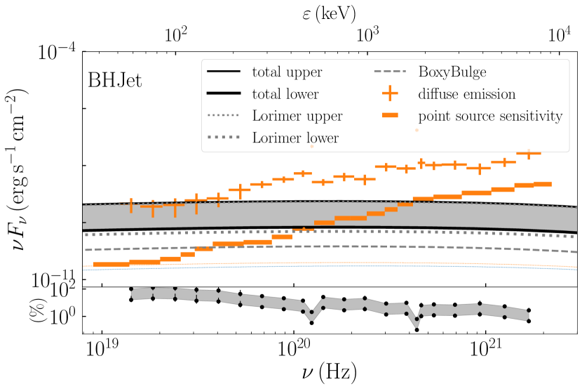
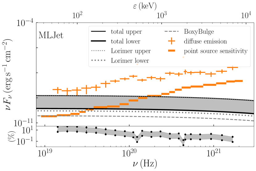
Figure 6: Similar to Fig. 5 but for the energy band covered by INTEGRAL for $(|l|,|b|)\leq(47.5^{\circ},47.5^{\circ})$ (Berteaud et al., 2022). On top of the diffuse emission, we plot the point source sensitivity of INTEGRAL/SPI as indicated in the legend (Roques et al., 2003) and compare it to individual sources that contribute to the total emission (solid colourful lines for individual sources). We show only those sources that are above the instrument sensitivity. Note that there are no sources above the threshold for MLJet.

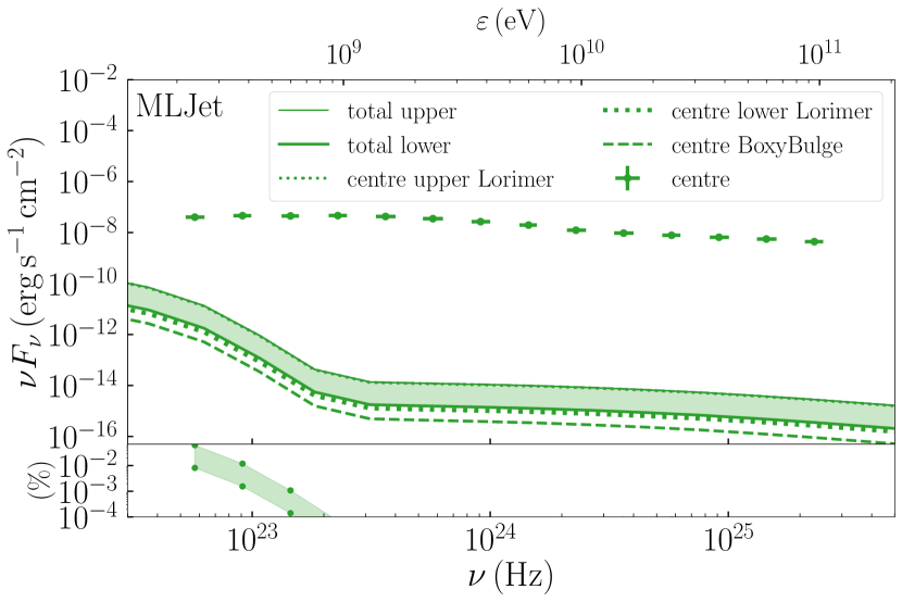
Figure 7: Similar to Fig. 5 but for the energy band covered by Fermi/LAT, and only for the region around the GC with $|l|\leq 80^{\circ}$ and $|b|\leq 8^{\circ}$.

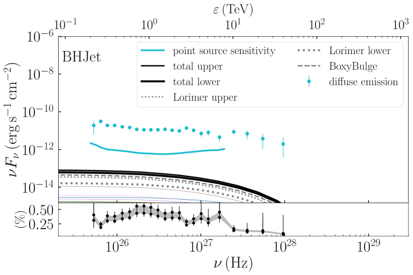
(a) H.E.S.S.

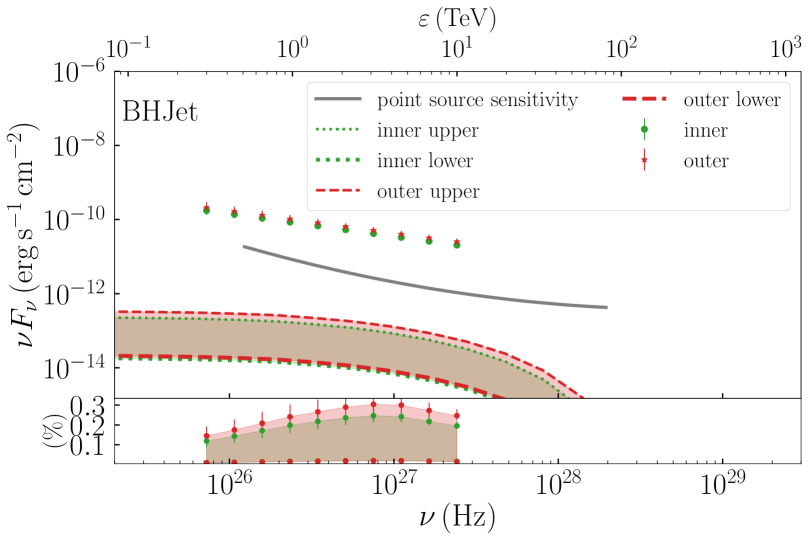
(b) HAWC

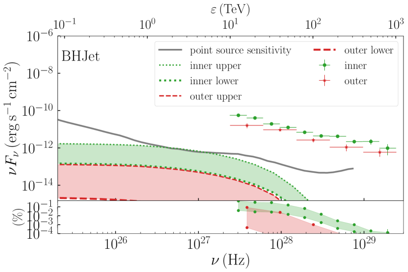
(c) LHAASO

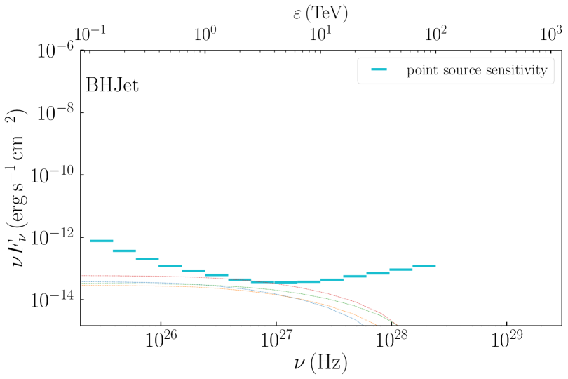
(d) CTA

Figure 8: Similar to Fig. 5, but for the highest energy regime of TeV comparing to H.E.S.S., HAWC, LHAASO and CTA facilities (from (a) to (d) panel, respectively). For H.E.S.S., HAWC, and LHAASO, we show with solid colourful lines the individual sources that exceed $10^{-3}$ of the point source sensitivity, and for CTA, we show those that exceed 1/3rd of the predicted point source sensitivity. For all panels, we only show the case of BHJet because the contribution of sources that follow MLJet is even less than pictured here. The inner (outer) region for the case of HAWC is $43^{\circ}\leq l\leq 73^{\circ}$ and $|b|\leq 2^{\circ}$ ($|b|\leq 4^{\circ}$), and the inner (outer) region for the case of LHAASO is $15^{\circ}\leq l\leq 125^{\circ}$ ($125^{\circ}\leq l\leq 235^{\circ}$) and $|b|\leq 5^{\circ}$. For CTA, the sources are within $|l|\leq 60^{\circ}$ and $|b|\leq 3^{\circ}$ (Eckner et al., 2023). All the panels have the same axes for comparison.

4.2 Multi-wavelength prompt emission

In Figs. 5–8, we plot the cumulative emission of all these qBHXBs in different energy bands from keV X rays to TeV $\gamma$ rays. More precisely, we use the detected diffuse emission from the following instruments to investigate the contribution of qBHXBs: NuSTAR in the keV band, INTEGRAL in the $\sim$MeV X rays, Fermi/LAT in the GeV $\gamma$ rays, H.E.S.S., HAWC, LHAASO and CTA for TeV $\gamma$ rays. Moreover, we compare individual sources to the instrument sensitivity to discuss their potential detection.

We use the NuSTAR Galactic diffuse emission from Perez et al. (2019) for a region of $3^{\circ}$ around the GC. For the case of INTEGRAL, we adopt the analysis of Berteaud et al. (2022) for $\lvert\rm{l}\lvert\leq 47.5^{\circ}$ and $\lvert\rm{b}\lvert\leq 47.5^{\circ}$ for the diffuse emission, and the sensitivity from Roques et al. (2003). The Fermi/LAT data for different regions in the sky map are from Ackermann et al. (2012), and for four different regions: the Galactic disc with $\lvert\rm{l}\lvert\leq 80^{\circ}$ and $\lvert\rm{b}\lvert\leq 8^{\circ}$, the intermediate for $\lvert\rm{l}\lvert\leq 180^{\circ}$ and $10^{\circ}\leq\lvert\rm{b}\lvert\leq 20^{\circ}$, the ridge with $80^{\circ}\leq\lvert\rm{l}\lvert\leq 180^{\circ}$ and $\lvert\rm{b}\lvert\leq 8^{\circ}$, and the region off plane with $\lvert\rm{l}\lvert\leq 180^{\circ}$ and $8^{\circ}\leq\lvert\rm{b}\lvert\leq 90^{\circ}$. The H.E.S.S. diffuse emission is from H.E.S.S. Collaboration et al. (2018) for a region of $\lvert\rm{l}\lvert\leq 1^{\circ}$ and $\lvert\rm{b}\lvert\leq 5^{\circ}$. The best fit of the HAWC Galactic diffuse emission for $43^{\circ}\leq\rm{l}\leq 73^{\circ}$ and two regions on the skymap with $\lvert\rm{b}\lvert\leq 2^{\circ}$ for the innermost one, and $\lvert\rm{b}\lvert\leq 4^{\circ}$ for the outermost one, are $8.89\pm 0.37^{-0.70}_{+0.48}\times\left(E/7.0\,\rm{TeV}\right)^{-2.612\pm 0.030^{-0.036}_{+0.015}}$ and $5.45\pm 0.25^{-0.44}_{+0.38}\times\left(E/7.0\,\rm{TeV}\right)^{-2.604\pm 0.034^{-0.037}_{+0.012}}$ in units of $10^{-12}\,\rm{TeV^{-1}\,s^{-1}\,cm^{-2}\,sr^{-1}}$, respectively (Alfaro et al., 2024), fixing for a probable typo in the units provided. The HAWC sensitivity after 507 days is derived from Abeysekara et al. (2017). For the $\sim$PeV regime and the LHAASO collaboration, there are two sky map regions with $\lvert\rm{b}\lvert\leq 5^{\circ}$, the innermost one with $15^{\circ}\leq\rm{l}\leq 125^{\circ}$ and the outermost with $125^{\circ}\leq\rm{l}\leq 235^{\circ}$ (Cao et al., 2023). Finally, we adopt the CTA simulated sensitivity for $\lvert\rm{l}\lvert\leq 60^{\circ}$ and $\lvert\rm{b}\lvert\leq 3^{\circ}$ from Eckner et al. (2023). For each different energy regime, we only use those sources that are within the aforementioned regions to calculate the cumulative emission.

In Fig. 5, we show the predicted cumulative emission of both the Lorimer distribution and the Boxy Bulge in the keV spectrum. For simplicity, we neglect the GC because it does not contribute almost at all. In the upper panel, we show the cumulative emission assuming that all the qBHXBs obey to the BHJet model, and in the lower panel the MLJet. As we mentioned already, the $1.2\times 10^{5}$ sources of Olejak et al. (2020) are those sources that host a BH with a non-degenerate companion, but not necessarily all of these BHs accrete matter from the companion at the same time. We hence use this value as an upper limit (densely dotted line labelled as ‘Lorimer upper’), and we combine it with a lower limit assuming that 10% of these sources accrete at a time (see further discussion below). Summing up the Boxy Bulge with either the upper limit of the Lorimer or the lower limit yields the total emission in the keV X-ray band between some upper and some lower limits (total upper and total lower, respectively). The grey-shaded region, hence, shows the total predicted emission from the Galactic qBHXBs between the upper limit of the Lorimer and some lower case of 10%. In the sub-panels of both upper and lower panels, we show the percentage of the potential contribution of the qBHXBs to the NuSTAR diffuse emission. For both jet models and depending on the number of disc sources, the contribution might be of the order of a few to 20%.

In Fig. 6, we plot the contribution of the qBHXBs to the INTEGRAL diffuse emission (orange crosses) following the above pattern. The contribution of qBHXBs to this energy band is larger, reaching values of almost 100% in the $\sim 100$ keV to a few % in the tens of MeV. In the same plots, we include the sensitivity of INTEGRAL/SPI for point sources from Roques et al. (2003) to compare to individual sources. For the case of BHJet, we find that a few sources might exceed the sensitivity in the first couple of energy bins in the $\sim$40-100 keV.

In Fig. 7, we plot the predicted contribution of qBHXBs to the GeV $\gamma$ rays compared to Fermi/LAT detection of the extended region around the GC. Once more, we use the same pattern as above to derive the upper limit of the total emission assuming an upper limit for the Lorimer-like disc distribution, and a smaller fraction of that at 10%. The overall contribution drops to less than 0.1% in these energy bins, and in fact, for the case of the BHJet the contribution drops below $10^{-4}$% at energies beyond GeV. For MLJet on the other hand, the contribution can be of the order of 0.1% not only in the GeV energies but also in the 100 GeV. In Appendix A, we show the predicted contribution of qBHXBs at intermediate Galactic latitudes, the ridge and off plane, for both BHJet and MLJet. We see no more than 0.1% in the 1 GeV and 100 GeV energy bins, similar to the GC.

Finally, in Fig. 8 we combine the three operating TeV facilities of H.E.S.S., HAWC and LHAASO, with the under-construction next-generation facility of CTA. qBHXBs can contribute up to 0.5% of the 1-10 TeV diffuse emission detected by H.E.S.S., but no individual sources are expected to be detected by H.E.S.S. (no individual sources exceed the plotted sensitivity). The qBHXBs of the ridge, so only sources from the disc, can contribute up to 0.3% in the TeV diffuse emission detected by HAWC, and up to 0.1% in the 10 TeV emission detected by LHAASO. For LHAASO, and the outer region, in particular, where $125^{\circ}\leq l\leq 235^{\circ}$, the contribution drops as a function of energy and falls below $10^{-4}$%. Finally, in Fig. 8, we compare some individual sources that we find that may produce significant TeV emission close to $10^{-13}\,\rm erg\,s^{-1}\,cm^{-2}$ with the predicted CTA sensitivity for point source detection in the Galactic plane. In Fig. 8, we only include the predicted emission from qBHXBs using the BHJet jet model because the case of MLJet yields some TeV emission that is significantly lower and hence, the overall contribution drops significantly even less than $10^{-4}$ percent, a threshold that we adopt here.

4.3 CR fluxes and multi-wavelength secondary emission

In the above, we have only accounted for the intrinsic emission from the jets of qBHXBs for either BHJet or MLJet. This intrinsic radiation is the product of the non-thermal CRs accelerated within the jets. When these CRs, or more precisely a fraction of these CRs, escape the acceleration sites, they propagate in the Milky Way. Using numerical means to keep track of this propagation, we estimate the CR flux detected here on Earth, and we compare it to the detected spectrum. In particular, we use DRAGON2, a publicly available simulator of the Galactic propagation. We assume that the CR sources are the same as above, namely a Gaussian population around the GC, a Boxy Bulge, and a Lorimer-like disc distribution. The normalisation of each distribution is thoroughly explained in Appendix B. Each qBHXB ejects some CRs in the Milky Way that follow a power law in energies similar to the intrinsic one, and carry some total power that we show in Table 2. Moreover, we calculate the maximum of the CR energy to be of the order of 20 TeV (see Table 2). As we show in Appendix C, the contribution of the propagated protons is less than $10^{-10}$, and for electrons is of the order of $10^{-12}$.

Table 2: The calculated power carried by the non-thermal protons (p) and electrons (e), and their maximum energy, for the two jet models we examine.

	BHJet	MLJet
$P_{p}\,(10^{33}\,\rm erg\,s^{-1})$	$310$	$4$
$P_{e}\,(10^{33}\,\rm erg\,s^{-1})$	$17$	$11$
$E_{p}$ (TeV)	$17$	$30$
$E_{e}$ (TeV)	$20$	$13$

5 Discussion

5.1 BHJet vs MLJet for A0620–00

To finally find out what is the exact number of qBHXBs in the Milky Way, and what is their role in the multi-wavelength emission, we need to better investigate the physics of individual sources, such as A0620–00. With both BHJet and MLJet jet models, we capture the broadband electromagnetic picture from radio to X rays. More precisely, the thermal synchrotron emission from the jet base can explain the IR emission along with the stellar emission of the companion, in agreement with Dinçer et al. (2017). The synchrotron optically thick emission connects the radio to the X-ray emission, similar to various BHXBs in outburst (Merloni et al., 2003; Falcke et al., 2004; Plotkin et al., 2014). In both cases, though, we see that the IC contributes equally, so it is impossible to distinguish the two components with merely spectral fitting, and further means are needed, such as timing analysis. Nonetheless, we manage to constrain the jet dynamics to predict the hard X-ray and $\gamma$-ray emission. In both scenarios and assuming an efficient particle acceleration, we see that the optically thick synchrotron emission reaches the MeV bands emerging from a cooled population of non-thermal electrons. The distribution of these electrons is the convolution of a thermal Maxwell-Jüttner and a non-thermal tail that expands to energies of the order of 10 TeV (see Table 2), for a power-law index close to 2 (see Table 1). This distribution is similar to the one plotted in Fig. 6 of K22 but for a softer index. The radiation footprint of such a leptonic population to tens of TeV energies, is the flat spectrum in the keV-MeV regime in a $\nu F_{\nu}(\nu)$ plot (see the Syn, $z>z_{\rm diss}$ component of Fig. 2). This sub-MeV emission is hard to be detected by either INTEGRAL or Fermi/LAT under such jet conditions.

The main differences between the two jet models are in the GeV and beyond spectrum, and in the jet composition. Starting from the latter, for BHJet we assume an equal number density of electrons and protons all along the jet. For MLJet on the other hand, as we describe in Sec. 2, the jets are launched with $\eta$ pairs of electrons and positrons with respect to pairs of electrons and protons. For A0620–00, we use this as a free parameter, and we find that $\sim$200 pairs per proton are needed to explain the radio-to-X-ray emission. Such a difference in the jet composition leads to different spectral components in the TeV band. In particular, the neutral pion decay from pp interactions is reduced in the case of MLJet because fewer targets reside in the jets to allow for inelastic collision, but more target electrons exist allowing for a stronger IC component (stronger compared to BHJet but still not enough to increase significantly the GeV flux). Such a more physically motivated proton power allows for better constraints in terms of jet energetics, but unfortunately does not lead to stronger non-thermal $\gamma$-ray emission.

5.2 Population of BHXBs in the disc

According to Olejak et al. (2020), $1.2\times 10^{5}$ qBHXBs may reside in the Galactic disc, but this number is very uncertain. However, only a fraction of these sources are expected to accrete and launch jets simultaneously nowadays. Based on the radio detection of another qBHXB, namely VLA J2130+12, Tetarenko et al. (2016a) estimate that $2.6\times 10^{4}-1.7\times 10^{8}$ objects may exist in the Milky Way at the moment. The lower limit is of the same order of magnitude as the value that we use in this work as a lower limit of the current qBHXBs (for simplicity we use $1.2\times 10^{4}$ sources, namely 10% of the total population). That many qBHXBs could be in agreement with the more recent observations of Gaia that detected approximately $6\times 10^{3}$ ellipsoidal systems, with a few % of them harbouring a compact object (Gomel et al., 2023). Gaia has however detected only nearby binaries, and only those with an orbital period smaller than a few days to be able to safely claim that they are indeed binaries.

The estimated lower limit of Tetarenko et al. (2016a) is consistent with the upper limit of theoretical predictions for the number of BHXBs in the Milky Way based on population synthesis (see, e.g. Romani 1992; Portegies Zwart et al. 1997; Kalogera & Webbink 1998; Pfahl et al. 2003; Yungelson et al. 2006; Kiel & Hurley 2006). Nonetheless, in the population synthesis studies the fraction of accreting BHXBs is typically of the order of $\sim 0.01$ % within a Hubble time (Yungelson et al., 2006). More recent analysis by Wiktorowicz et al. (2019) shows that $\sim 10^{4}$ BHXBs should fill their Roche lobe, a value that is only 1% of the total population of sources.

The estimated upper limit of Tetarenko et al. (2016a) is approximately two orders of magnitude above the upper limit we use in this work. As we see in Figs. 5 and 6, the X-ray diffuse emission does not allow for more than $10^{5}$ jetted qBHXBs at the same time. A further comparison, however, might not lead to concrete conclusions because our main assumption that all these $1.2\times 10^{4}-1.2\times 10^{5}$ qBHXBs launch jets of approximately the same power, cannot rule out the existence of even more qBHXBs but without any jet emission at all. Consequently, the contradiction between the theoretical prediction of $\leq 10^{4}$ and the observational evidence for $\geq 10^{4}$ is worth revisiting to allow us to better constrain the contribution of (q)BHXBs to the observed diffuse Galactic radio to $\gamma$-ray emission detected, and vice versa, the further observational investigation of (q)BHXBs can help to better constrain the contribution of these sources to the Galactic diffuse emission.

5.3 X-ray to $\gamma$-ray contribution to the diffuse emission

The diffuse X-ray emission detected by NuSTAR is mainly up to 90% due to cataclysmic variables (Perez et al., 2019). There is some 10% however that is due to unresolved Galactic sources. In this work, we find that qBHXBs that launch jets can contribute up to 10% depending on the jet model. The contribution can be reduced to a few percent, respectively, given that the number of accreting qBHXBs drops to 10 percent, namely of the order of $1.2\times 10^{4}$ sources in the Galactic disc.

In the more energetic X-ray regime, and in particular, in the energy window observed by INTEGRAL, we find that the qBHXBs can fully explain the $\sim 100$ keV band and up to a few% to the tens of keV regime. It is worth mentioning that in the X-ray analysis of the INTEGRAL data, the contribution of the unresolved sources is usually assumed to follow a power-law in energy with an exponential cutoff (see, e.g. Berteaud et al., 2022), but based on this analysis we see that the contribution of qBHXBs is energy dependent, and is dropping with energy. This energy dependence of the contribution is due to radiative-cooled electrons accelerated in the qBHXBs jets. In the case of less efficient particle acceleration where the particles escape the acceleration sites way before reaching their theoretical maximum energy, the X-ray spectrum would show a cutoff at much smaller energies than tens of MeV, but still in the X-ray band. The contribution of qBHXBs to the high-energy tail may hence drop, unlike the lower regime at 100  keV.

In the softer regime of the MeV X-ray spectrum, when we compare the INTEGRAL sensitivity for individual sources to the predicted emission of some individual qBHXBs that contribute the most to the diffuse emission, we see that for the case of BHJet we expect one source at most to be detected in the 30-100 keV regime. To yield a more accurate prediction of that value, we performed 250 realisations of our simulations to find on average $0.4\pm 0.5$ sources to be detected by INTEGRAL. Such a value is indeed in good agreement with the number of BHXBs detected by INTEGRAL so far, however, no qBHXB has been detected yet.

In the higher energy regime of $\gamma$ rays, we see that the contribution of qBHXBs is less than 1% in the entire spectrum from GeV to TeV energies. CTA, however, is expected to be 10 times more sensitive than current facilities. To make a stronger prediction for this energy regime, we realized 250 simulations yielding $1\pm 0.5$ sources to be detected by CTA. It is worth remarking that these sources are merely in the quiescence and not during outburst when stronger TeV emission is expected (see, e.g. Kantzas et al. 2023). Keeping track of these sources that exceed the CTA sensitivity in each realisation of the simulations, we see that CTA will be able to detect sources that are located closer than $\sim 2\,$kpc (with an average distance of $0.9\pm 0.4\,$kpc) and have a viewing angle less than $17^{\circ}$ (with an average viewing angle of $11\pm 2^{\circ}$). The majority of the BHXBs known so far are beyond 1 kpc with the nearest system to be at 0.5 kpc (El-Badry et al., 2022; Chakrabarti et al., 2023). Regarding the viewing angle, only MAXI J1836–194 has a viewing angle less than 15^∘ located further than 4 kpc (Russell et al., 2014). It is worth noting that we obtain these results under the assumption that all qBHXBs follow the spectral behaviour of A0620–00 because the number of qBHXBs that have good quality multi-wavelength data are still limited. If CTA manages indeed to detect TeV emission from individual qBHXBs, this will allow us to study a new part of the parameter space.

5.4 Radio counterparts and predictions for future facilities

The radio counterpart of qBHXBs, such as the one detected by VLA from A0620–00 (Dinçer et al., 2017), is a key element to prove the jet emission, particularly in the case of a flat radio spectrum (Blandford & Königl, 1979). Current facilities such as VLA and MeerKAT can detect sources with radio intensity as low as less than 100$\mu$Jy, sometimes reaching values close to 10$\mu$Jy (Driessen et al., 2019; Goedhart et al., 2024), and in the future with ngVLA (Butler et al., 2019) and the full array of SKA (Braun et al., 2017), the threshold for detection may drop to $\sim\mu$Jy. In Fig. 9, we plot the distribution of sources per energy flux at $1.28\,GHz$. The two different histograms correspond to the assumption of the upper/lower Lorimer distribution, similar to above. We show that for the current threshold of the order of $\sim 10\mu$Jy, we may be able to detect up to $\sim$20-80 sources, depending on the number of jetted qBHXBs (lower and upper limits, respectively). Simultaneous multi-wavelength observations in the optical and/or the X rays, as well as timing analysis that hints for periodicity, are necessary to identify such radio sources as (q)BHXBs (see e.g. Driessen et al., 2019).

Figure 9: The distribution of sources per energy flux detected at a characteristic radio frequency of 1.28 GHz. The two different histograms correspond to the two different assumptions for an upper or lower limit of qBHXBs populating a Lorimer-like distribution in the disc. We show for comparison the detection threshold of radio sources with current facilities, such as MeerKAT and VLA ($\sim 10\mu$Jy).

5.5 Neutrino counterpart

The recent Galactic neutrino diffuse emission detected by IceCube strengthens the idea of the existence of non-thermal accelerators in the Galactic plane (IceCube Collaboration et al., 2023). The hadronic processes that can take place in the jets of BHXBs lead to the formation of non-thermal astrophysical neutrinos that reach energies of the order of a few tens of TeV. To find the possible contribution of the qBHXBs to the detected Galactic neutrinos, we estimate self-consistently the neutrino emission from each individual source for all the three source populations we study here. In Fig. 10, we plot the total neutrino flux expected from the qBHXBs in the Milky Way, and we compare it to the detected Galactic diffuse emission. More precisely, the detected neutrino spectrum is model-dependent, and assuming three different CR propagation models, IceCube Collaboration et al. (2023) derive three different neutrino spectra. The $\pi^{0}$ corresponds to the CR propagation model of Galprop that uses as a normalisation the Fermi/LAT observations of the diffuse $\gamma$-ray emission (Ackermann et al., 2012), whereas the KRA_γ model corresponds to the CR propagation for which the diffusion coefficient is spatially dependent and there is an exponential cutoff in the propagating CR power-law at 5 or 50 PeV (KRA${}_{\gamma}^{5}$ and KRA${}_{\gamma}^{50}$, respectively; Gaggero et al. 2015).

We show only the case of BHJet because neutrino emission in the MLJet scenario is further suppressed (see discussion above for $\gamma$ rays). We find the total contribution of qBHXBs to the detected spectrum to be less than 1% at energy of the order of 1-2 TeV that rapidly drops to even less than $10^{-2}$% at energy around 10 TeV.

Figure 10: The predicted neutrino flux from the source populations as shown in the legend (also see Fig. 5), assuming that the BHJet jet scenario explains their jet dynamics. The subplot shows the contribution of the total predicted flux to the detected Galactic neutrino diffuse emission by IceCube (IceCube Collaboration et al., 2023) with the three different colours to represent the three different models used to extract the observed flux.

6 Summary and Conclusions

BHXBs have recently been revised as Galactic CR sources. The majority of these objects spend their lifetime in quiescence, with only a handful of those to be detected from radio to X rays. Recent observations of qBHXBs suggest the existence of relativistic jets that can accelerate particles to high energies. In this work, based on the well-studied qBHXB A0620–00 we examine this scenario. We use in particular two different jet models, BHJet and MLJet, and we find that both can sufficiently explain the radio-to-X-ray electromagnetic spectrum. Non-thermal relativistic electrons may reach energies of the order of tens of TeV that lead to some strong synchrotron and IC emission that can explain the X-ray spectrum. Regardless of the acceleration of protons to non-thermal energies, we find that no significant $\gamma$-ray radiation from this source is produced to be detected by current or planned facilities.

The exact number of BHXBs and qBHXBs is under debate, with observations and simulations yielding values that range between a few thousand up to $10^{8}$. Following the population synthesis analysis of Olejak et al. (2020), we examine the contribution of $1.2\times 10^{4}-1.2\times 10^{5}$ qBHXBs to the CR spectrum and the X-ray/$\gamma$-ray Galactic diffuse emission. While no significant contribution is expected in both the electron and proton CR spectra detected on Earth, we find that the cumulative intrinsic emission of these objects can significantly contribute to the Galactic diffuse emission. More precisely, assuming that all the qBHXBs have the same spectral behaviour as A0620–00 but rescaled for the distance and viewing angle, we derive the predicted spectrum from X rays to $\gamma$ rays. We find that for a population of $10^{4}$ sources located in the Boxy Bulge and between $1.2\times 10^{4}-1.2\times 10^{5}$ in the Galactic disc, qBHXBs can explain up to 10% of the keV X-ray spectrum depending on the jet conditions. This contribution is the maximum, and more conservative numbers of qBHXBs can reduce the contribution to a few %. The soft MeV Galactic diffuse emission is expected to be dominated by cataclysmic variables and IC of CR electrons, qBHXBs however can contribute up to 10-90 percent, depending on the jet dynamics and the exact value of sources. We find moreover that the contribution of qBHXBs to the unresolved hard MeV spectrum is dropping with energy because the emission originates in the non-thermal synchrotron of radiatively cooled electrons. This is a feature that may help to better identify the origin of the MeV diffuse emission. The radio counterpart of qBHXBs may reveal their exact number. Current radio facilities that are sensitive to $\sim 10\,\rm\mu Jy$, such as MeerKAT, could detect up to tens of qBHXBs that can better constrain their absolute number in the Milky Way. In the more energetic regime, CTA will detect a couple of these sources, in particular those that reside at distances less than 2 kpc and with viewing angles less than $15^{\circ}$ to allow for further boosting. Only recently we have started detecting such sources at distances as close as 0.5  kpc and sources with viewing angles as low as $\sim 10^{\circ}$, hence further observations would help to better constrain the contribution of BHXBs and qBHXBs in particular, to the CR spectrum and the Galactic diffuse emission. Finally, qBHXBs may explain up to 1% of the diffuse neutrino background as detected by IceCube with their contribution dropping significantly at neutrino energies beyond $\sim 10\,$TeV.

Appendix A Fermi spectra

In Fig. 11, we plot the contribution of the qBHXBs to the $\gamma$-ray spectrum and compare it to the Fermi/LAT diffuse emission. See Fig. 7 for details.

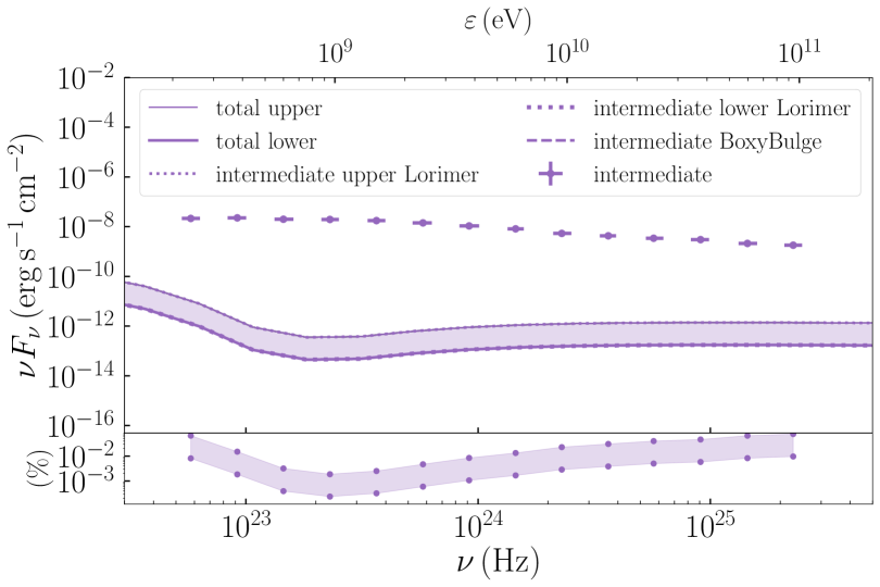
(a) Intermediate Galactic coordinates and BHJet

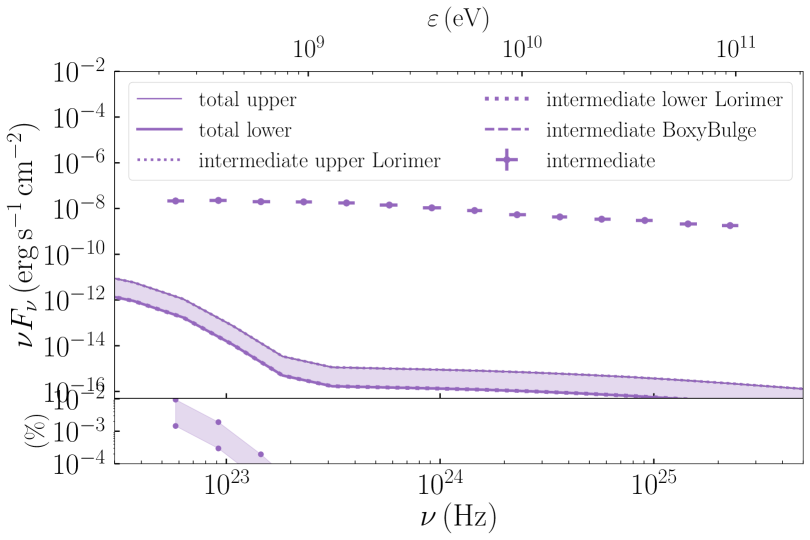
(b) Intermediate Galactic coordinates and MLJet

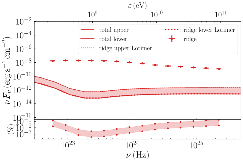
(c) The Galactic ridge and BHJet

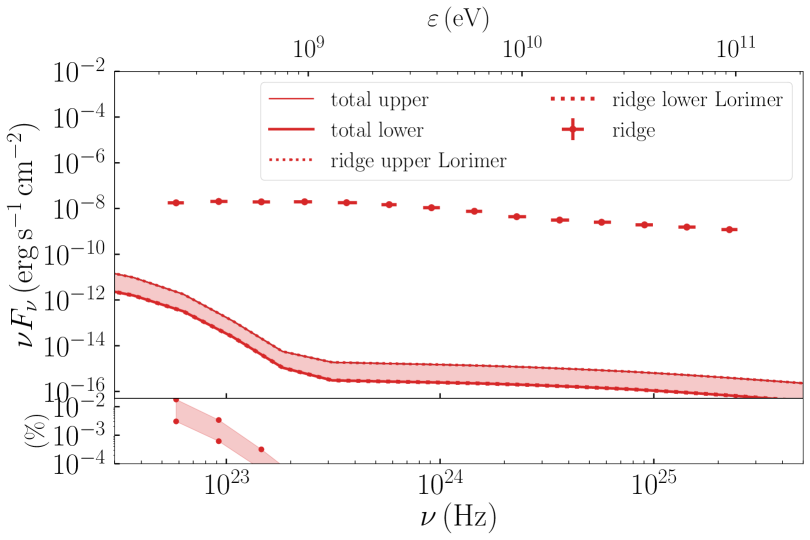
(d) The Galactic ridge and MLJet

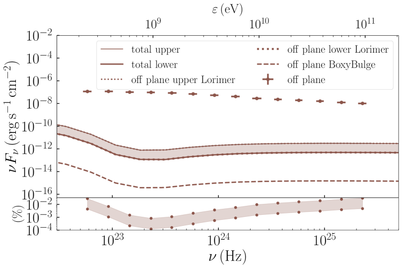
(e) Off the Galactic plane and BHJet

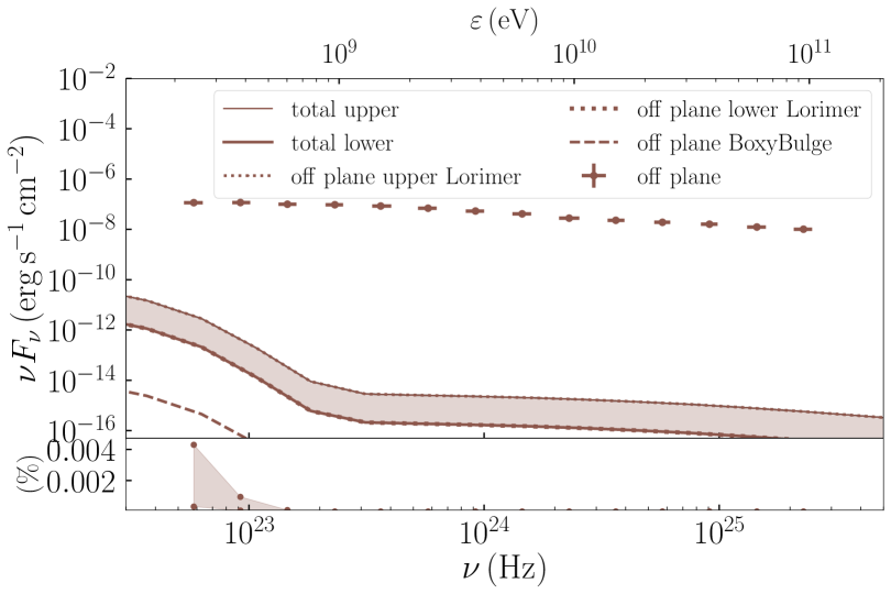
(f) Off the Galactic plane and MLJet

Figure 11: Similar to Fig. 7 but for the Fermi/LAT detection of intermediate Galactic coordinates $10^{\circ}\leq|b|\leq 20^{\circ}$ in the upper panels, for the Galactic ridge with $80^{\circ}\leq|l|\leq 180^{\circ}$ and $|b|\leq 8^{\circ}$ in the middle panels, and off plane $|b|\geq 8^{\circ}$ in the lower panels.

Appendix B DRAGON2 population setup

The total number of sources is the sum of the sources in the disc $N_{d}$, the sources located in the central parsec region $N_{c}$ add those in the bulge $N_{b}$:

$$N_{\rm total}=N_{d}+N_{c}+N_{b}.$$ (1)

Each population follows a distribution:

$$N=\int_{0}^{\infty}N_{0}\rho(R)\xi(z)dV,$$ (2)

where $N_{0}$ is the normalisation of each population, and $\rho(R)$ and $\xi(z)$ are the (unitless) number densities in the radial direction and perpendicular to the Galactic plane, respectively.

The disc sources follow the profile of the Lorimer distribution (Lorimer et al., 2006):

$$\rho_{d}(R)\xi_{d}(z)=\left(\frac{R}{R_{0}}\right)^{B}e^{-C(R-R_{0})/R_{0}}\,e^{-|z|/\varepsilon},$$ (3)

where $R_{0}=8.3$kpc, $B=1.9$, $C=5$, and $\varepsilon=0.18$kpc. The normalisation of the Lorimer distribution is hence given by:

$$\begin{split}N_{0,d}&=\frac{N_{d}}{\dfrac{2\pi R_{0}^{2}\varepsilon}{C^{B+2}e^{-C}}\bigintss_{\ 0}^{\infty}t^{B+1}e^{-t}dt,}\\ &=\frac{N_{d}C^{B+2}e^{-C}}{2\pi R_{0}^{2}\varepsilon\ \Gamma(B+2)Q(B+2,0)}.\end{split}$$ (4)

where we set $t=cR/R_{0}$, $\Gamma$ is the Euler (gamma) function and $Q$ is the generalized incomplete gamma function.

The sources of the Galactic centre follow a Gaussian distribution (Mori et al., 2021) whose the normalisation is:

$$N_{0,c}=\frac{N_{c}}{\sqrt{2\pi}\varepsilon\left[2\sigma_{c}e^{-\mu_{c}^{2}/4\sigma_{c}^{2}}+\sqrt{\pi}\mu_{c}\left(\textrm{erf}\left(\dfrac{\mu_{c}}{2\sigma_{c}}\right)+1\right)\right]},$$ (5)

where $\mu_{c}=2\,$pc, $\sigma_{c}=20\,$pc and erf is the error function. This normalisation yields $N_{0,c}=98040\times\dfrac{N_{c}}{1000}$.

Finally, the sources of the bulge follow a spherical distribution (Korol et al., 2018):

$$\rho_{b}(r)=e^{-r^{2}/2r_{b}^{2}},$$ (6)

where $r_{b}=0.5\,$kpc is the characteristic radius of the bulge and $r=\sqrt{R^{2}+z^{2}}$ is the spherical distance from the Galactic centre. The normalisation of this distribution is:

$$N_{0,b}=\frac{N_{b}}{4\pi\left(\sqrt{2}r_{b}\right)^{3}\bigintss_{\ 0}^{\infty}x^{2}e^{-x}dx}=\frac{N_{b}}{8\pi\left(\sqrt{2}r_{b}\right)^{3}}.$$ (7)

In a Cartesian 3D coordinate system, and for a more realistic distribution, we use the boxy bulge (Cao et al., 2013) that is described by the modified Bessel function of the second kind $K_{0}(r_{s})$ where

$$r_{s}=\left(\left(\left(\frac{x}{x_{0}}\right)^{2}+\left(\frac{y}{y_{0}}\right)^{2}\right)^{2}+\left(\frac{z}{z_{0}}\right)^{4}\right)^{1/4},$$ (8)

with $x_{0}=0.69\,$kpc, $y_{0}=0.29\,$kpc and $z_{0}=0.27\,$kpc. The normalisation for the 3D boxy bulge can be written as $N_{0,BB}=7420\times\frac{N_{BB}}{10000}$. For all the normalisations we assume the Milky Way to extend to some radius of 12 kpc and height 4 kpc.

We define the fraction of sources that are located in the GC with respect to the total number of sources:

$$\varepsilon=\frac{N_{c}}{N_{\rm total}},$$ (9)

which we allow to vary.

The total source luminosity is

$$\begin{split}L_{\rm CR}&=\int N_{0}\rho(R)\xi(z)dV\int G(p)Q_{0}(p)f(E,p)dEdp,\\ &=N_{\rm total}\int\phi(f_{\rm esc})f_{\rm esc}\ P_{\rm p}df_{\rm esc},\end{split}$$ (10)

where $f_{\rm esc}$ is the fraction of CRs escaped from the jets of each individual source, $\phi(f_{\rm esc})$ is the PDF of $f_{\rm esc}$ and $P_{\rm p}$ is the power carried by the protons, which according to A0620–00 is $8.9\times 10^{34}\,\rm erg\,s^{-1}$. We calculate $N_{0}$ from the total number of sources

$$\begin{split}N_{0}&=\frac{N_{\rm total}}{\bigintss\rho(R)\xi(z)2\pi RdRdz},\\ &=N_{\rm total}\left(\dfrac{N_{c}}{N_{0,c}}+\dfrac{N_{d}}{N_{0,d}}+\dfrac{N_{b}}{N_{0,b}}\right)^{-1},\end{split}$$ (11)

and $f(E)$ is the energy distribution of the particles of each source, which we assume to be a power-law $E^{-p}$ with an exponential cutoff at some maximum energy $E_{\rm max}$. The power-law index is around 2, and we assume that its probability density follows a Gaussian $G(p)$ with $\mu_{p}=2.0$ and $\sigma_{p}=0.3$ (cite particle acceleration papers here). In DRAGON2 we use as an input the quantity $N_{0}Q_{0}$ (Q0_custom), so we calculate $Q_{0}$ as

$$Q_{0}(p)=\dfrac{\bigintss\phi(f_{\rm esc})f_{\rm esc}\ P_{p}df_{\rm esc}}{\bigintss f(E,p)dE}.$$ (12)

For the case of a power law $f(E)=E^{-p}$ from $E_{p,\rm min}=1\,\rm GeV$ to $E_{p,\rm max}=36\,\rm TeV$ (see Section where we describe the jet model and how we calculate the maximum energy for protons)

Appendix C CR spectrum

In Fig. 12, we plot the proton CR spectrum where we show the contribution of the qBHXBs to the detected spectrum. We compare to AMS-02 proton spectrum (Aguilar et al., 2015), the ATIC proton data (Chang et al., 2008), the CREAMIII (Yoon et al., 2017), DAMPE (DAMPE collaboration et al., 2019), and KASCADE (Apel et al., 2011). The qBHXBs mainly from the disc (because the Boxy Bulge GeV-TeV protons are subdominant) contribute very insignificantly, with less than $10^{-10}$. In Fig. 13 we show the electron CR spectrum using the AMS-02 electron data (Aguilar et al., 2014), and similar to protons, the contribution is negligible. In the same plot, we show the contribution of both the primary electrons and those produced by the propagation of protons and their interaction with the Galactic gas. We see that the secondary electrons dominate over the primary, but still are not enough to contribute somehow to the detected electron spectrum.

Figure 12: The contribution of the qBHXBs of a Lorimer-like distribution in the Galactic disc to the proton CR spectrum as detected on Earth. For comparison, we include the contribution of the BHXBs in the hard state from Kantzas et al. (2023).

Figure 13: The contribution of a Lorimer-like distribution of qBHXBs in the Galactic disc to the electron CR spectrum detected on Earth. We plot both the primary electrons (dotted line), namely those that escape the qBHXBs and propagate in the Galaxy, and the secondary electrons that are formed after the inelastic collisions of the propagating proton CRs with the Galactic gas (dotted line).