Constrained dynamics and confinement in the two-dimensional quantum Ising model
Abstract
We investigate the dynamics of the quantum Ising model on two-dimensional square lattices up to spins. In the ordered phase, the model is predicted to exhibit dynamically constrained dynamics, leading to confinement of elementary excitations and slow thermalization. After demonstrating the signatures of confinement, we probe the dynamics of interfaces in the constrained regime through sudden quenches of product states with domains of opposite magnetization. We find that the nature of excitations can be captured by perturbation theory throughout the confining regime, and identify the crossover to the deconfining regime. We systematically explore the effect of the transverse field on the modes propagating along flat interfaces and investigate the crossover from resonant to diffusive melting of a square of flipped spins embedded in a larger lattice.
While interacting quantum systems typically relax to equilibrium relatively quickly, there are striking examples where this is not the case [1, 2]. Investigating the origins of the anomalously long prethermal regime of such systems has applications in understanding exotic phases of condensed matter [3, 4], phenomena like false vacuum decay [5] and quark confinement [6].
One possible reason for slow thermalization is the emergence of dynamical constraints which approximately restrict the time evolution to certain subspaces of the full Hilbert space. A prominent example are systems with confinement [7], where pairs of elementary excitations experience attraction which increases with increasing separation, and thus form long-lived bound states. This is, for example, the reason why quarks at low temperatures do not exist as isolated particles, but are bound in mesons or hadrons.
An analogous mechanism is also found in Ising spin chains [8]. At small transverse fields, the low energy excitations are domain walls, and pairs of them feel a confining force provided by the longitudinal field [9, 10, 11, 12, 13] or interactions beyond nearest neighbour [14]. The direct correspondence between confined domain walls in spin systems and pairs of charges confined by a gauge field in lattice gauge theories makes the Ising chain a useful toy model for studying thermalization of bound states via meson production [15, 16, 17, 18]. Domains of spins anti-aligned with the longitudinal field are bubbles of false vacuum, and probing their dynamics is crucial for understanding false vacuum decay [19, 20].
In two dimensions (2D), the confining potential comes from the lattice itself. An excitation has to flip neighbouring spins to propagate, thus adding domain walls. At small transverse fields such processes are very energetically costly, and thus strongly suppressed. Confinement has initially been studied in ladders [21, 22], by orthogonally coupling many chains described by the Ising field theory in the scaling limit [23, 7] and recently in a 2D lattice with infinite tensor network methods [24]. These approaches describe the system in the thermodynamic limit and hence cannot probe dynamics of inhomogeneous initial states and domain walls.
In this paper, we use tree tensor networks (TTNs) to explore the constrained dynamics of the quantum Ising model on 2D square lattices of up to spins, through quenches of product states to finite transverse fields. Starting with the completely polarized state, we demonstrate signatures of confinement and investigate the nature of low-energy excitations that drive the dynamics. Then, we turn our attention to two representative types of domain walls, a flat interface between two spin species and a square domain embedded in a larger lattice, to explore the melting of interfaces in the confining regime. We characterize the surface modes that are known to dominate the dynamics in the limit of small transverse field [25, 26], and investigate the crossover towards diffusive melting. We find that the crossover corresponds to the dynamical phase transition from the ordered to disordered phase and we characterize the nature of domain melting in both regimes. Finally, we discuss the feasibility of implementing our numerical calculations on quantum simulators and suggest an outlook of possible extensions of the presented work.
Model and methods - The Hamiltonian of the two-dimensional quantum Ising model is
| (1) |
with - and -Pauli matrices and , the interaction, and the transverse field strength. Sum indices run over sites of a square lattice, with indicating a sum over nearest neighbours. We choose to work with periodic boundary conditions throughout, but the physics observed here does not depend on this choice.
Throughout the paper, we investigate instantaneous quenches of product states with spins aligned in the -direction (eigenstates at ) to finite values of . We encode them into tree tensor networks [27, 28, 29] and propagated in real time using the time-dependent variational principle (TDVP) [30, 31], with a timestep of . Our results are generally sufficiently converged for the maximal bond dimension . See Supplemental Material (SM) for technical details and convergence analysis.
Broadly speaking, the accuracy of tensor network methods is bound by entanglement. After instantaneous quenches of product states it typically grows, at worst linearly with time [32]. This means that the resources required for accurate tensor network calculations grow exponentially. However, as shown in this work and elsewhere [9, 7, 24], the physical regime investigated here is noteworthy precisely because entanglement grows slowly in time. This makes TTNs a particularly apt tool to attack the present problem.
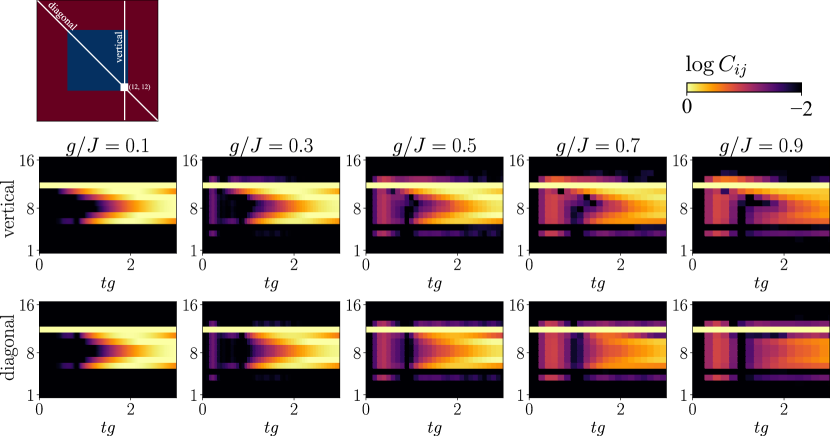
We characterize the physics through various observables. Aside from the local magnetization , we use the spin-spin correlation function where and are lattice sites of the two spins. When quenching from a product state where initially for all , the time evolution of quantifies the spread of an excitation in time.
The entanglement of two parts of the system is quantified through the von Neumann entropy , where are the singular values of the Schmidt decomposition of the chosen bipartition. is also a measure of the spread of excitations across the bipartition, as this process entangles the two parts of the system.
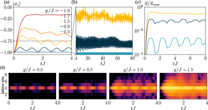
Confinement - Slow thermalization of a many-body system is reflected in persistent oscillations of local observables, like the magnetization of one spin. Additionally, a striking signature of confined dynamics is the suppression of the light-cone spread of correlations, and slow and non-monotonous growth of entanglement with time [9]. We start by demonstrating these properties after a quench of a completely polarized product state to finite . The time dependence of the magnetization is presented in Figs. 1(a,b). For small , we find persistent oscillations with no signs of suppression up to large times. However, when increasing towards , equilibrates on a timescale of . This indicates the onset of a regime of quick thermalization, in rough agreement with the critical value of the transverse field for a dynamical phase transition in the same model, [33].
The time evolution of the entanglement entropy is shown in Fig. 1(c). We choose a bipartition between two neighbouring spins and the rest of the system, but all other bipartitions produce similar results. At small , we observe an oscillatory pattern with the system periodically returning very close to a product state with a frequency of approximately . Interestingly, the frequency is half the frequency of the oscillations of . The oscillations are washed out as is increased and the density of excitations becomes large enough that they interact, leading to thermalization [34].
The spin-spin correlations also exhibit signatures of confinement, see Fig. 1(d), where we plot a vertical cut of with spin chosen in the fourth row. The spread of correlations is strongly suppressed for small . At , we find non-monotonous behaviour with the same frequency as the oscillations of entanglement. The light-cone component becomes more apparent as is increased, and at it is clearly the dominant contribution. It should be mentioned that the light-cone never vanishes completely, but is only suppressed. Its apparent disappearance is an artefact of the choice of a plotting scale [9, 14].
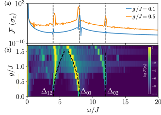
Nature of excitations - The oscillating behaviour of local observables implies that the dynamics is generated by repeated creation and annihilation of local excitations. Their nature can be inferred from the spectral density of local observables [9, 34, 14, 24]. In Fig. 2 we show the results of the Fourier transform of the magnetization from Fig. 1(b) between and , denoted by . We multiply the timeseries by the Hamming window to exclude possible transient events at the edges of the interval [35, 36]. An example of the spectral density for two values of is shown in Fig. 2(a), while a heatmap for a broader range is in Fig. 2(b).
The three peaks match the excitation energies of the dominant dynamical processes. The most prominent peak, starting at for , corresponds to the transition between the initial state and a state with one flipped spin, . The peak at corresponds to a transition between and , a state where two neighbouring spins are flipped, with a total domain wall length of . Finally, the peak at is produced by the transition between and .
The -dependence of the excitation energies can be captured by perturbative corrections to the product states. The expressions up to the second order in are:
| (2) |
Note that is the linear size of our system, which consists of sites in total. For complete calculations see the SM.
The black dashed lines in Fig. 2(b) indicate the transition energies obtained as differences of these energies, denoted . They match the positions of the spectral peaks to surprisingly large values of transverse field, up to . This is somewhat surprising for expressions which are technically only accurate up to the second order in , and indicates that the contribution of the higher excited modes is negligible throughout the confining regime.
Note that aside from the extensive correction common to all states, we do not find a second-order contribution to . An intuitive interpretation is that in second order the corrections that come from coupling to , and the ones coming from (superposition of connected three-spin clusters, total domain length of 8), originate from the same physical process, ie. adding or removing a spin from an existing cluster. Both add two domain walls, and being symmetric in this sense, they cancel out. The processes that couple to only appear at fourth order, and we expect that accounting for those would reproduce the curvature of the right and left peaks in Fig. 2(b).
The spectrum of excitations hints at the underlying reasons for quick thermalization beyond . The peak indicates the cost of flipping a spin next to an already existing spin flip – growing a spin cluster by one. Quenching to the point where this process is energetically as expensive as creating a single spin flip populates not only the first few but also higher excited states, resulting in the formation of larger clusters and thus thermalization on a timescale of .
Because the dynamics of confined systems is dominated by low energy excitations, it can be accurately described by a simple effective model [16, 14, 24]. This is typically done by projecting the Hamiltonian to a subspace of low-energy excitations (equivalents of our , and ). However, this approach leads to certain inconsistencies. Namely, the matrix element between the ground and first excited state is extensive (indeed, in our case we find ), while others are independent of . Therefore, an effective model including predicts a spectral gap (equivalent of that diverges with system size. To accurately reproduce the excitation energies, the initial vacuum state (equivalent of ) should be excluded from the low energy model, and its mass set exactly to zero.
Perturbative calculations imply that the origin of the problem is in the arbitrary truncation of the subspace of the effective model (see SM for details). We find that the extensive corrections come from a state coupling to an extensive number of excitations with one more and one fewer spin flip – it is always possible to flip a decoupled spin in approximately places for an energy penalty of . The contributions coming from the state with one more and one less spin flip cancel out in the perturbative calculations, and we only find an overall correction to all states, so that energy differences remain independent of system size. However, if the Hilbert space is first truncated into an effective model, the coupling between the last retained and the first truncated state is not taken into account, the extensive contributions do not cancel out, and the gaps grow with system size. While the two approaches produce a similar energy diagram, an advantage of the perturbative approach is that it can also provide corrections to the eigenstates.
Interfaces - Next, we probe the dynamics of interfaces by investigating quenches of inhomogeneous initial states. We consider two examples: the stripe, an initial state where two domains of opposite polarized spins are separated by a flat interface, and the square, where the flipped spins are arranged into a square domain.
Confinement importantly affects interface dynamics. Whereas interfaces are typically expected to diffusively melt, in the confining phase they tend to remain stable up to very long times. This is because classically resonant processes dominate the dynamics for small , ie. only spins with two neighbours of each spin species can flip, as the initial and final state have the same energy. These processes only locally reshape the domain wall, and thus its total length emerges as a dynamic constraint. The interface dynamics is well understood in the limit of infinite where non-resonant processes are explicitly forbidden [25, 26]. Slow thermalization comes as a consequence of the subsequent fragmentation of Hilbert space into sectors labeled by the domain wall length, and further into so-called dynamically decoupled Krylov subspaces; two domains cannot merge through local reshaping of the interface if they are separated by multiple lattice sites [37, 38].
Results for the stripe are presented in Fig. 3, with a sketch of the initial state shown in Fig. 3(a). Recall the periodic boundary conditions, which ensure that the interface is completely flat with no kinks.
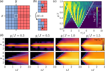
In this case, the lowest excitation above the initial state is a spin flip at the interface. It creates two additional domain walls and costs . However, once this excitation is present, flipping the neighbouring interface spin does not come with any additional energy penalty, see Fig. 3(b). Such excitations are thus allowed to freely propagate along the boundary, with the expected dispersion [39].
The spectral density of for a spin at the interface is shown in Fig. 3(b). The most prominent feature is the excitation which starts at for and fans out into a continuum with increasing , as expected of a freely propagating mode. White dashed lines correspond to the expected envelopes of the transition energies . The continuum is split into discrete peaks as a consequence of the finite size of the lattice.
Vertical and horizontal cuts of the connected correlation functions are shown in Fig. 3(c). Because of the interface, the spread of correlations is not the same in the horizontal and vertical directions. In the horizontal direction (orthogonal to the interface) correlations show signatures of confinement equivalent to results in Fig. 1. Interestingly, the correlation spread is symmetric, meaning that the confined excitations spread across the interface into the domain with opposite polarisation in the same way as within the domain. On the other hand, the vertical (y) cuts show very different behaviour. The freely propagating interface mode spreads the correlations along the interface with a velocity proportional to (blue dashed lines in Fig. 3(c)), even for . As is further increased the dynamics lose their - asymmetric nature, and at large correlations spread equally in either direction.
Finally, we consider the melting of an square of spins embedded in a lattice and surrounded by spins. Fig. 4(a) shows snapshots of magnetization for small and intermediate , while Fig. 4(b) shows the time dependence of magnetization for a set of spins close to a corner of the square. For extended plots of magnetization as well as correlation spread, see the SM.
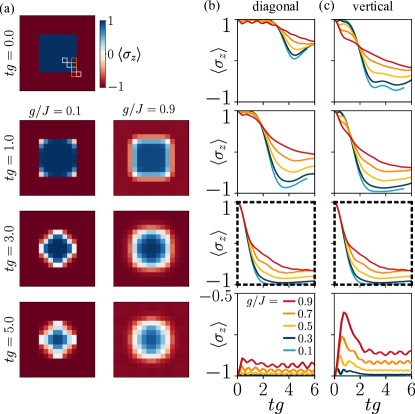
As shown in Refs. [25, 26], in the limit and for an infinitely large corner the melting process can be understood as a series of resonant spin-flip processes. Because the corner spin has two neighbours of each spin species it flips on a timescale set by . After the corner spin is flipped, its two neighbours can resonantly flip as well. This triggers a propagating edge mode in the same way as in Fig. 3. The process is illustrated in the magnetization snapshots for in Fig. 4(a), and results in the square melting into a cross-like shape.
A more quantitative view is presented in Figs. 4(b,c). At small the edge mode dominates. For spins along the interface shown in panel (c), the delay of melting is thus linear in the distance from the corner. Probing deeper into the square along the diagonal (Fig. 4(b)), we find that spins near the center stay inert up to relatively long times. Note that here we rescale time with , and find that the small curves in Fig. 4(b,c) follow the same trend. This indicates that the smaller energy scale dominantly drives the dynamics.
Increasing causes deviations from this simple picture and a crossover towards a regime where all spins at the interface melt simultaneously. The amplitude of magnetization oscillations is gradually reduced, and at we find a monotonous decrease of for all spins of the square simultaneously. The melting produces waves of magnetization radiating from sides of the square into the environment (see bottom panel of Fig. 4(c), and SM extended plots). This is a sign that the dynamics is no longer confined, and that the length of the domain wall is not conserved.
Realization on a quantum simulator - The Ising model is naturally realized in various quantum simulation platforms. However, being two-dimensional, the presented setup is most directly applicable to neutral atom arrays and within reach of existing experiments. More concretely, Ref. [40] demonstrates control over 2D arrays of hundreds of Rydberg atoms realizing a nearest-neighbour antiferromagnetic Ising model with the interaction on the order of MHz and coherence time of s. When driving the transition between the two spin states at around Mhz, the timescales shown in Fig. 4 correspond to experimental times of a few microseconds. If one chose to relax the nearest neighbour constraint the atoms could be moved much closer together, leading to stronger interactions and thus much faster dynamics. See for example Ref. [41] for an experimental and Ref. [42] for a similar theoretical proposal.
Outlook - We used tree tensor networks to study constrained dynamics in the ordered phase of the two-dimensional quantum Ising model. We showed the signatures of confinement of quasiparticles and extracted the spectrum of excitations from oscillations of the magnetization. The spectrum can be adequately reproduced by perturbation theory up to , while the failure at larger is related to thermalization. Then, we investigated the melting of interfaces of domains with opposite spins, how it depends on confinement and how it changes with increasing transverse field. We find a crossover between the constrained dynamics of classically resonant processes in the limit of small and diffusive melting at large .
An important implication of the presented work is the fact that these classical simulations are possible up to such long times. The underlying reason is slow entanglement growth and thus slow increase of bond dimension required to retain the accuracy of tensor network states. The confining regime is thus perfect for benchmarking quantum machines with tensor network calculations [24].
We see various other open questions that could be addressed either on a quantum simulator, or with minimal alterations of our setup. One interesting avenue is the exploration of Floquet dynamics through quenches with a time-dependent transverse field. Because relatively long timescales are reachable, it is possible to investigate the regime of small and intermediate frequencies, and thus explore the regime beyond the corrections of the Magnus expansion. Floquet dynamics have recently been studied in a related system, where a discrete time crystal was identified in the prethermal state [43].
Another option is to investigate false vacuum decay. In two dimensions, dynamical confinement and the presence of false vacuum are decoupled – confinement is provided by the lattice, while the false vacuum is invoked by a longitudinal field. A starting point would be to investigate how the melting in Fig. 4 depends on longitudinal field, which makes the square either a false or a true vacuum domain.
Expanding on this idea, it would be interesting to probe the scattering of false vacuum bubbles. Such calculations have been performed in one dimension [44], but many more scattering channels are expected to arise in two dimensions. However, to clearly discern scattering from lattice effects one would have to significantly increase the system size, possibly beyond the reach of classical simulations.
Acknowledgements.
We acknowledge enlightening discussions with Marcello Dalmonte, Roberto Verdel, Simone Notarnicola, Jernej Rudi Finžgar, and Sourav Nandy. The authors acknowledge funding from CN00000013 - Italian Research Center on HPC, Big Data and Quantum Computing (ICSC), the H2020 projects EuRyQa, QuantERA2017 project QuantHEP, QuantERA2021 project T-NiSQ, the Quantum Technology Flagship project PASQuanS2, the Italian Ministry of University and Research (MUR) via PRIN2022 project TANQU, the Departments of Excellence grant 2023-2027 Quantum Frontiers, the German Federal Ministry of Education and Research (BMBF) the funding program quantum technologies, project QRydDemo, and the World Class Research Infrastructure - Quantum Computing and Simulation Center (QCSC) of Padova University. The simulations were performed using the Quantum Green Tea software version 0.3.23 and Quantum Tea Leaves version 0.4.46 [45]. The authors acknowledge computational resources of the HPC center Vega at the Institute of Information Science (IZUM) in Maribor, Slovenia and HPC Leonardo by Cineca, Italy.References
- Polkovnikov et al. [2011] A. Polkovnikov, K. Sengupta, A. Silva, and M. Vengalattore, Colloquium: Nonequilibrium dynamics of closed interacting quantum systems, Reviews of Modern Physics 83, 863–883 (2011).
- De Roeck and Verreet [2019] W. De Roeck and V. Verreet, Very slow heating for weakly driven quantum many-body systems (2019).
- Yang [1989] C. N. Yang, pairing and off-diagonal long-range order in a hubbard model, Physical Review Letters 63, 2144–2147 (1989).
- Moudgalya et al. [2020] S. Moudgalya, N. Regnault, and B. A. Bernevig, -pairing in hubbard models: From spectrum generating algebras to quantum many-body scars, Physical Review B 102, 10.1103/physrevb.102.085140 (2020).
- Coleman [1977] S. Coleman, Fate of the false vacuum: Semiclassical theory, Physical Review D 15, 2929–2936 (1977).
- Greensite [2020] J. Greensite, An Introduction to the Confinement Problem (Springer International Publishing, 2020).
- James et al. [2019] A. J. A. James, R. M. Konik, and N. J. Robinson, Nonthermal states arising from confinement in one and two dimensions, Phys. Rev. Lett. 122, 130603 (2019).
- McCoy and Wu [1978] B. M. McCoy and T. T. Wu, Two-dimensional Ising field theory in a magnetic field: Breakup of the cut in the two-point function, Physical Review D 18, 1259–1267 (1978).
- Kormos et al. [2016] M. Kormos, M. Collura, G. Takács, and P. Calabrese, Real-time confinement following a quantum quench to a non-integrable model, Nature Physics 13, 246–249 (2016).
- Mazza et al. [2019] P. P. Mazza, G. Perfetto, A. Lerose, M. Collura, and A. Gambassi, Suppression of transport in nondisordered quantum spin chains due to confined excitations, Physical Review B 99, 10.1103/physrevb.99.180302 (2019).
- Vovrosh and Knolle [2021] J. Vovrosh and J. Knolle, Confinement and entanglement dynamics on a digital quantum computer, Scientific Reports 11, 10.1038/s41598-021-90849-5 (2021).
- Tan et al. [2021] W. L. Tan, P. Becker, F. Liu, G. Pagano, K. S. Collins, A. De, L. Feng, H. B. Kaplan, A. Kyprianidis, R. Lundgren, W. Morong, S. Whitsitt, A. V. Gorshkov, and C. Monroe, Domain-wall confinement and dynamics in a quantum simulator, Nature Physics 17, 742–747 (2021).
- Magoni et al. [2021] M. Magoni, P. P. Mazza, and I. Lesanovsky, Emergent bloch oscillations in a kinetically constrained Rydberg spin lattice, Physical Review Letters 126, 10.1103/physrevlett.126.103002 (2021).
- Liu et al. [2019] F. Liu, R. Lundgren, P. Titum, G. Pagano, J. Zhang, C. Monroe, and A. V. Gorshkov, Confined quasiparticle dynamics in long-range interacting quantum spin chains, Physical Review Letters 122, 10.1103/physrevlett.122.150601 (2019).
- Pichler et al. [2016] T. Pichler, M. Dalmonte, E. Rico, P. Zoller, and S. Montangero, Real-time dynamics in U(1) lattice gauge theories with tensor networks, Physical Review X 6, 10.1103/physrevx.6.011023 (2016).
- Verdel et al. [2020] R. Verdel, F. Liu, S. Whitsitt, A. V. Gorshkov, and M. Heyl, Real-time dynamics of string breaking in quantum spin chains, Physical Review B 102, 10.1103/physrevb.102.014308 (2020).
- Lerose et al. [2020] A. Lerose, F. M. Surace, P. P. Mazza, G. Perfetto, M. Collura, and A. Gambassi, Quasilocalized dynamics from confinement of quantum excitations, Physical Review B 102, 10.1103/physrevb.102.041118 (2020).
- Verdel et al. [2023] R. Verdel, G.-Y. Zhu, and M. Heyl, Dynamical localization transition of string breaking in quantum spin chains, Physical Review Letters 131, 10.1103/physrevlett.131.230402 (2023).
- Lagnese et al. [2021] G. Lagnese, F. M. Surace, M. Kormos, and P. Calabrese, False vacuum decay in quantum spin chains, Physical Review B 104, 10.1103/physrevb.104.l201106 (2021).
- Pomponio et al. [2022] O. Pomponio, M. A. Werner, G. Zaránd, and G. Takacs, Bloch oscillations and the lack of the decay of the false vacuum in a one-dimensional quantum spin chain, SciPost Physics 12, 10.21468/scipostphys.12.2.061 (2022).
- Ramos et al. [2020] F. B. Ramos, M. Lencsés, J. C. Xavier, and R. G. Pereira, Confinement and bound states of bound states in a transverse-field two-leg Ising ladder, Physical Review B 102, 10.1103/physrevb.102.014426 (2020).
- Lagnese et al. [2022] G. Lagnese, F. M. Surace, M. Kormos, and P. Calabrese, Quenches and confinement in a Heisenberg–Ising spin ladder, Journal of Physics A: Mathematical and Theoretical 55, 124003 (2022).
- Konik and Adamov [2009] R. M. Konik and Y. Adamov, Renormalization group for treating 2D coupled arrays of continuum 1D systems, Physical Review Letters 102, 10.1103/physrevlett.102.097203 (2009).
- Tindall and Sels [2024] J. Tindall and D. Sels, Confinement in the transverse field Ising model on the heavy hex lattice (2024).
- Balducci et al. [2022] F. Balducci, A. Gambassi, A. Lerose, A. Scardicchio, and C. Vanoni, Localization and melting of interfaces in the two-dimensional quantum Ising model, Physical Review Letters 129, 10.1103/physrevlett.129.120601 (2022).
- Balducci et al. [2023] F. Balducci, A. Gambassi, A. Lerose, A. Scardicchio, and C. Vanoni, Interface dynamics in the two-dimensional quantum Ising model, Physical Review B 107, 10.1103/physrevb.107.024306 (2023).
- Shi et al. [2006] Y.-Y. Shi, L.-M. Duan, and G. Vidal, Classical simulation of quantum many-body systems with a tree tensor network, Physical Review A 74, 10.1103/physreva.74.022320 (2006).
- Silvi et al. [2019] P. Silvi, F. Tschirsich, M. Gerster, J. Jünemann, D. Jaschke, M. Rizzi, and S. Montangero, The Tensor Networks Anthology: Simulation techniques for many-body quantum lattice systems, SciPost Physics Lecture Notes 10.21468/scipostphyslectnotes.8 (2019).
- Cataldi et al. [2021] G. Cataldi, A. Abedi, G. Magnifico, S. Notarnicola, N. D. Pozza, V. Giovannetti, and S. Montangero, Hilbert curve vs Hilbert space: exploiting fractal 2D covering to increase tensor network efficiency, Quantum 5, 556 (2021).
- Bauernfeind and Aichhorn [2020] D. Bauernfeind and M. Aichhorn, Time dependent variational principle for tree tensor networks, SciPost Physics 8, 10.21468/scipostphys.8.2.024 (2020).
- Haegeman et al. [2016] J. Haegeman, C. Lubich, I. Oseledets, B. Vandereycken, and F. Verstraete, Unifying time evolution and optimization with matrix product states, Physical Review B 94, 10.1103/physrevb.94.165116 (2016).
- Eisert and Osborne [2006] J. Eisert and T. J. Osborne, General entanglement scaling laws from time evolution, Physical Review Letters 97, 10.1103/physrevlett.97.150404 (2006).
- Hashizume et al. [2022] T. Hashizume, I. P. McCulloch, and J. C. Halimeh, Dynamical phase transitions in the two-dimensional transverse-field Ising model, Physical Review Research 4, 10.1103/physrevresearch.4.013250 (2022).
- Lin and Motrunich [2017] C.-J. Lin and O. I. Motrunich, Quasiparticle explanation of the weak-thermalization regime under quench in a nonintegrable quantum spin chain, Physical Review A 95, 10.1103/physreva.95.023621 (2017).
- win [2024] Window function — Wikipedia, the free encyclopedia (2024), [Online; accessed 28-May-2024].
- Harris [1978] F. Harris, On the use of windows for harmonic analysis with the discrete fourier transform, Proceedings of the IEEE 66, 51 (1978).
- Yoshinaga et al. [2022] A. Yoshinaga, H. Hakoshima, T. Imoto, Y. Matsuzaki, and R. Hamazaki, Emergence of hilbert space fragmentation in Ising models with a weak transverse field, Physical Review Letters 129, 10.1103/physrevlett.129.090602 (2022).
- Hart and Nandkishore [2022] O. Hart and R. Nandkishore, Hilbert space shattering and dynamical freezing in the quantum Ising model, Physical Review B 106, 10.1103/physrevb.106.214426 (2022).
- Mbeng et al. [2020] G. B. Mbeng, A. Russomanno, and G. E. Santoro, The quantum Ising chain for beginners (2020).
- Scholl et al. [2021] P. Scholl, M. Schuler, H. J. Williams, A. A. Eberharter, D. Barredo, K.-N. Schymik, V. Lienhard, L.-P. Henry, T. C. Lang, T. Lahaye, A. M. Läuchli, and A. Browaeys, Quantum simulation of 2D antiferromagnets with hundreds of Rydberg atoms, Nature 595, 233–238 (2021).
- Bluvstein et al. [2021] D. Bluvstein, A. Omran, H. Levine, A. Keesling, G. Semeghini, S. Ebadi, T. T. Wang, A. A. Michailidis, N. Maskara, W. W. Ho, S. Choi, M. Serbyn, M. Greiner, V. Vuletić, and M. D. Lukin, Controlling quantum many-body dynamics in driven Rydberg atom arrays, Science 371, 1355–1359 (2021).
- Samajdar and Huse [2024] R. Samajdar and D. A. Huse, Quantum and classical coarsening and their interplay with the Kibble-Zurek mechanism (2024).
- Shinjo et al. [2024] K. Shinjo, K. Seki, T. Shirakawa, R.-Y. Sun, and S. Yunoki, Unveiling clean two-dimensional discrete time quasicrystals on a digital quantum computer (2024).
- Milsted et al. [2022] A. Milsted, J. Liu, J. Preskill, and G. Vidal, Collisions of false-vacuum bubble walls in a quantum spin chain, PRX Quantum 3, 10.1103/prxquantum.3.020316 (2022).
- Ballarin et al. [2024] M. Ballarin, G. Cataldi, A. Costantini, D. Jaschke, G. Magnifico, S. Montangero, S. Notarnicola, A. Pagano, L. Pavešić, M. Rigobello, N. Reinić, S. Scarlatella, and P. Silvi, Quantum TEA: qtealeaves (2024).
Supplementary Material
Numerical details
The numerical calculations presented in this work are performed with tree tensor networks (TTNs) [27, 28]. In this appendix, we provide qualitative reasoning for the utility of TTNs compared to other tensor networks and technical aspects of the algorithm for time evolution that we apply, and present plots of magnetization and entanglement obtained for a set of maximal bond dimensions.
Tree tensor networks
In TTNs, the state is represented by a tensor network in the shape of a symmetric binary tree, where the bottom tensors (’leaves’ of the tree) carry the physical indices. The tree tensor network ansatz is particularly successful at describing states where distant sites are entangled, such as in chains with long-range interactions. The reason why can be understood through a qualitative picture of the way quantum states are encoded in tensor networks. Qualitatively, entanglement between two correlated physical states is transferred through bonds of the network that connect them. The more entanglement there is, the bigger the bond dimension required to accurately describe the state. Generally, this also means entangled states are better represented by tensor networks with a bigger number of links. An extreme example of this is the projected entangled-pair state (PEPS) ansatz, where the tensor network mimics the structure of the 2D lattice and each tensor is directly connected to its nearest neighbours. However, this introduces loops in the network, which leads to technical difficulties. Namely, it is not possible to define the isometry center of a network with loops. Therefore, the algorithms for contracting such networks cannot rely on the underlying symmetries. This leads to poor scaling of calculations of local observables with bond dimension, and limits PEPS to bond dimensions on the order of . The TTN ansatz is in between the MPS and PEPS in the sense that it is the best connected tensor network which by construction has no loops. Furthermore, because two physical sites separated by lattice sites in real space are only separated by in the TTN, the entanglement between them is captured more efficiently.
Time evolution
The most common way to evolve tensor network states in time is with the time-dependent variatonal principle (TDVP) [30, 31]. The most popular is the two-tensor version of the algorithm (TDVP2), where at each step two neighbouring tensors are contracted, evolved in time, and then split and truncated via SVD. This algorithm can grow the bond dimensions between tensors at each time step and is thus a natural choice for simulations starting from weakly entangled states, such as the product states we use. A much faster version of the same concept is the single-tensor TDVP (TDVP1), where each tensor is optimized without contractions with the neighbours. In this case, the bond dimension cannot change, which presents a problem if the initial state is a product state with .
However, we find that the calculations are much faster if one pads the initial product state with numerical noise on the order of up to bond dimension , and we perform the evolution with TDVP1, without truncation. We find a speedup in computational time of about for a system at . We also tried hybrid approaches (like performing TDVP2 every th time step and TDVP1 otherwise, with around 10). The advantage here is that the initial bond dimension is not but rather gradually increases every -th step. This speeds up the initial time steps, but the advantage is quickly lost once the bond dimension reaches a sizeable fraction of the one used for TDVP1. An advantage might be expected for the easiest cases (small limit) where the bond dimension never reaches the maximal allowed value. However, these cases can also be accurately simulated by a TDVP1 simulation with smaller , which is anyway much faster. Furthermore, on a technical level having a single convergence parameter () is more desirable compared to having two ( and the minimal truncation ) with non-trivial interplay.
Another advantage of TDVP1 compared to TDVP2 is that the error of the latter is non-monotonous in the size of the time step. In TDVP2, an SVD and a truncation are performed at each time step. This introduces a truncation error, and thus choosing a time step that is too small might actually increase the total error. In TDVP1, there is no truncation, and the truncation error is exactly zero. Consequently, TDVP1 also exactly conserves the energy and norm of the evolved state.
Convergence
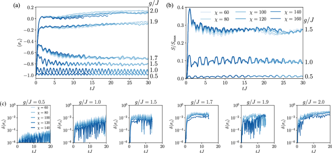
In Fig. 5, we show the convergence of (a) magnetization and (b) entanglement with increasing maximal bond dimension . The deviation of the magnetization at given with respect with the results obtained with are shown in Fig. 5(c).
The convergence is strongly dependent on the underlying physics. Deep in the confined phase at , results are well converged already for or less. At larger , larger is required to obtain well-converged results and the simulations become unreliable much sooner in simulated time.
We use for simulations of longer times, and find the magnetization results reliable up to . In simulations where we also want to ensure accurate convergence in entanglement and correlations, we use .
Perturbative corrections
This appendix contains calculations of the perturbative corrections up to the second order in for the first two excited states above the completely polarized ground state. We treat the interaction part as the unperturbed part
| (3) |
and the transverse field term as the perturbation
| (4) |
with running across the spins of the 2D system.
General remarks
The first-order perturbative corrections to energy of an unperturbed state are given by:
| (5) |
In our case, the unperturbed states are product states of spins polarized in , while only contains spin flipping terms . To obtain a non-zero overlap with the initial state, one has to flip at least two spins (or one spin twice), thus the first-order contributions will always be zero. The same argument applies to all odd-order corrections.
In the second order, the correction to a state is
| (6) |
where runs across all unperturbed eigenstates of the system that are not , being their unperturbed energy and the unperturbed energy of . In other words, is the sum of absolute values of all possible off-diagonal matrix elements weighted by the difference of the corresponding state’s energy with respect to .
In the case of the Ising model all off-diagonal matrix elements are the same, . To evaluate , we find all states which are a single spin flip away from , group them according to their energy , and count the number of such contributions.
Ground state
We are looking for the second order correction:
| (7) |
The matrix element is non-zero only for states with a single flipped spin, , with denoting the coordinates of the flip. Evidently, there are such states, each with the matrix element and excitation energy coming from the four domain walls.
The sum in Eq. (7) thus gives
| (8) |
First excited state
To find the -dependent correction to the excited states, we repeat the procedure for the state with one flipped spin. By examining the matrix elements , one notices that the only excited state coupled to is the zero-momentum superposition of spin flips
| (9) |
It is thus enough to evaluate the perturbative expansion only for this state. Again the first order correction , while in second order we have
| (10) |
with .
In this case, the non-zero contributions come from states with two spin flips:
| (11) |
Depending on the relative positions of and , there are three distinct classes of :
-
1.
; . There is exactly one such state, with intermediate energy .
-
2.
neighbours, denoted . There are such states (4 for each lattice site, but for double counting). Flipping neighbouring spins only creates 6 domain walls, thus the intermediate energy of this type of process is .
-
3.
neither neighbours nor equal, denoted . There are such states, again for double counting. The intermediate energy is .
Now, we compute the matrix elements for the three classes.
For , we have
| (12) |
and the total contribution to is
| (13) |
For the basis states with neighbouring flipped spins and , , we find
| (14) |
as the sum over and gives two ways to match the two flipped spins in . The total contribution of all such states to the energy shift is thus
| (15) |
Finally, for the matrix element is the same as above:
| (16) |
however, the intermediate energy is , and the number of states is bigger by a factor of , producing another extensive contribution to the energy shift:
| (17) |
The complete second-order energy correction is the sum of these terms:
| (18) |
Importantly, the extensive () contribution is the same as for the ground state, see Eq. (8), resulting in a -independent gap.
Second excited state
The second excited state is of type , with two neighbouring spins flipped. Again, it is enough to consider the zero-momentum superposition
| (19) |
with , neighbours.
The relevant classes of states coupled to have three spin flips over the ground state, . They are:
-
1.
two of , , equal, producing a state with a single flipped spin, . There is such states, and the intermediate energy is .
-
2.
, , and forming a connected three spin cluster, the state denoted . There are such clusters on a lattice. The intermediate energy comes from adding two domain walls, and is thus .
-
3.
disconnected from and , denoted . There are such states – for each , cluster the disconnected spin can be flipped on the remaining sites.
For the first case, we find the matrix element
| (20) |
In words, there are four ways to match any one flipped spin by starting from a superposition of all possible two-spin clusters and flipping one of them. The contribution to the correction is thus
| (21) |
In the second case, the matrix element is
| (22) |
Each connected three-spin cluster can be constructed by flipping a neighbouring spin of two distinct two-spin clusters. The total contribution is
| (23) |
Finally, the case of a decoupled flipped spin is similar to the third case of the corrections, but here with a different geometrical factor. The matrix element is
| (24) |
and thus the total contribution
| (25) |
When summing all contributions all -independent terms cancel out, and we obtain the second order correction to the energy of :
| (26) |
See the main text around Fig. 2 for a qualitative interpretation of the obtained result.
Additional results for the square
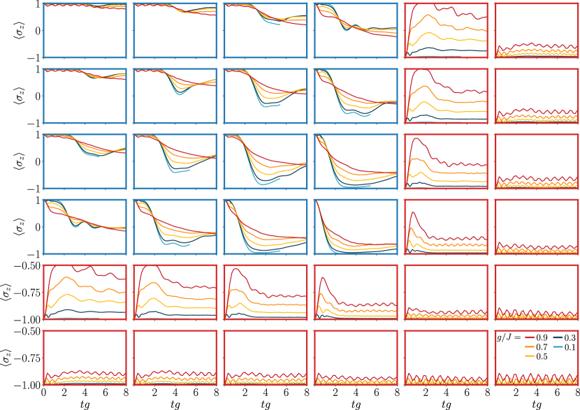
In this section, we provide additional results for the dynamics of the square. Fig. 6 shows a grid of magnetization for the lower right quadrant of the square (the panels with blue frames) and two surrounding rows and columns (red frames). Time is rescaled by , as in Fig. 4.
As discussed in the main text, we observe a crossover between two limiting behaviours; at small the dynamics consists of a sequence of resonant spin flips which originate from the corner, while with increasing the spins at the interface melt simultaneously. Spins within the square remain inert until the wave of melting reaches them. Interestingly, because the resonant process is a complete spin flip which propagates ballistically, the magnetization at intermediate times () generally reaches lower values for small , and the square seems to start melting more quickly. However, while the small- dynamics leads to multiple oscillations of magnetization, the large curves monotonously decay to their thermal value. Longer time simulations are required to accurately determine the nature of the thermalized state.
The diffusive dynamics at large spreads outside of the initial square, while it is confined to it at small . This is most apparent in the set of spins that neighbour the square, where we find a large initial jump of magnetization (note that the red-framed panels have a -scale from to ). Its magnitude increases approximately linearly with . For smaller the environment is effectively unperturbed at the scale shown here.
In Fig. 7, we show the correlations where is the spin in the corner of the square, and are taken along a vertical (top) or a diagonal (bottom) cut along the system. For we find the expected linear correlation spread along the side of the square, while it is somewhat slower along the diagonal. Interestingly, because the edge mode propagates much faster, the correlations with the spin in the opposite corner of the square begin growing approximately at the same time as the ones with the neighbouring spin along the diagonal.
As is increased, we find the expected light-cone spread, and the spread of correlations outside of the initial spread. An interesting feature that appears at larger are areas where decreases (at ). This is probably due to interference of signals propagating along different paths from the corner spin.