Edge Spin fractionalization in one-dimensional spin-$S$ quantum antiferromagnets

Abstract

We argue that the anisotropic quantum spin chain with spin $S$ (XXZ$-S$) exhibits exponentially localized fractional $\pm\frac{S}{2}$ edge modes in the gapped antiferromagnetic phase of the model. Moreover, we claim that this phenomenon is very general and exists in any $U(1)$ symmetric spin chain in its gapped antiferromagnetic regime with explicitly or spontaneously broken $\mathbb{Z}_{2}$ symmetry. We examine our argument for integrable and non integrable chains. By using the Bethe Ansatz method, we show that $XXZ-\frac{1}{2}$ and a $XXZ-1$ integrable chains have $\pm\frac{S}{2}$ fractionalized edge modes. Employing the density matrix renormalization group technique, we extend this analysis to generic XXZ-$S$ chains with $S\leq 3$ and demonstrate that these fractional spins emerge as robust quantum observables, substantiated by the observation of a variance of the associated fractional spin operators that is consistent with a vanishing functional form in the thermodynamic limit. Moreover, we find that the edge modes are robust to disorder that couples to the Néel order parameter.

Introduction: The concept of quantum fractionalization, initially demonstrated by Jackiw and Rebbi in continuous quantum field theory [1] and later extended to lattice systems by Su, Schrieffer, and Heeger [2], has now been found in various other systems. Notable manifestations include spin-charge separation [3, 4], fractional spin excitations in spin liquids [5, 6, 7, 8, 9, 10, 11], and the fractional quantum Hall effect [12, 13, 14, 15, 16, 17, 18]. It is well known theoretically that the exponentially localized fractional edge modes exist in systems with symmetry protected topological phases such as polyacetylene [2], the spin-1 Haldane chain [19, 20, 21], topological superconductors [22, 23, 24, 25, 26, 27, 28, 29], topological insulators [30, 31, 32, 33, 34, 35, 36, 37, 38, 39]. These topological edge modes and/or the fractional excitations have been experimentally observed in various natural and engineered systems including, fractional excitation in spin-$\frac{1}{2}$ antiferromagnet [40, 41], topological excitations in various systems [42, 43],topological edge modes in spin chains [44], topological edges state[45, 46, 47, 48], edge modes and surface states in topological insulators [49, 50, 51].

In this letter, we explicitly show that exponentially localized edge modes appear in other contexts that are associated with spontaneous or explicit breaking of discrete symmetries rather than topology. In particular, we consider the spin-$S$ quantum antiferromagnetic chain and we make the hypothesis that exponentially localized fractional spin $\pm\frac{S}{2}$ edge modes appear if the model satisfies (at least) the following three properties:

1. Antiferromagnetic order in the bulk due to explicitly or spontaneously broken $\mathbb{Z}_{2}$ symmetry,

2. $U(1)$ symmetry,

3. A finite bulk gap.

It is well known that strong zero modes exist in some spin chains [52, 53, 54, 55, 56]. Further, it was established that integrable anisotropic Heisenberg $XXZ-\frac{1}{2}$ chain with boundary fields in the gapped antiferromagnetic regime hosts fractionalized edge spins [57], which when projected onto the low energy subspace spanned by the ground state can be identified with the strong zero energy mode discussed in [53]. Here, we generalize it to arbitrary spin-$S$ chains which may or not be integrable and show that these edge modes are robust to short-ranged quenched disorder that couples to the order parameter. In the following, we consider the quantum Heisenberg spin-$S$ anisotropic chain defined by the Hamiltonian

$$H_{\Delta}=\sum_{i=1}^{N-1}(\vec{S}_{i}\cdot\vec{S}_{i+1})_{\Delta}=\sum_{i=1}^{N-1}S^{x}_{i}S^{x}_{i+1}+S^{y}_{i}S^{y}_{i+1}+\Delta S^{z}_{i}S^{z}_{i+1}.$$ (1)

where $S^{x}_{i},S^{y}_{i}$ and $S^{z}_{i}$ are the spin-$S$ operators that belong to the representation of $SU(2)$ at site $i$. We will consider several perturbations to this model that either satisfy or violate the three conditions defined in the introduction. The phase diagram of these models is well known [58] and is shown in Fig.1. Our hypothesis and focus applies to the antiferromagnetic regime i.e. $\Delta>1$ for half-integer $S$ and $\Delta>\Delta_{c_{2}}$ for integer $S$, where $\Delta_{c_{2}}>1$ is the boundary between the gapped Haldane phase and the gapped antiferromagnetic phase.

Figure 1: Phase diagrams of the XXZ-$S$ chains a) for integer spin and b) half-integer spin chain. In the integer chain there is a gapped topological phase between $\Delta_{c_{1}}<\Delta<\Delta_{c_{2}}>1$ between the gapless XY and gapped antiferromagnetic phase whereas in the half-integer chain there is a direct BKT transition from gapless XY phase to the gapped antiferromagnetic phase. As integer $S$ increases, $\Delta_{c_{2}}\to 1^{+}$ and $\Delta_{c_{1}}\to 1^{-}$ such that the value of $\Delta_{c_{2}}-\Delta_{c_{1}}$ decreases. Here we are only interested in the antiferromagnetic phase highlighted in the red color in each of the phase diagrams.

In the following, we first present two integrable cases for spin $1/2$ and $1$ that allow us to explicitly show the presence of fractionalized edge modes of spin $S/2$. We then use DMRG to further verify these edge modes are robust in XXZ spin chains up to spin $S=3$.

Integrable spin-1/2 and -1 Models: As a first example, we examine analytically tractable spin-1/2 $XX$ chain with a staggered magnetic field

$$H_{h}=\sum_{i=1}^{N-1}(-1)^{i}hS^{z}_{i}+(\vec{S}_{i}\cdot\vec{S}_{i+1})_{\Delta=0}.$$ (2)

Due to the staggered magnetic field, the model opens a gap and the antiferromagnetic order develops due to explicit breaking of the spin flip $\mathbb{Z}_{2}$ symmetry. Since this model can be mapped to free fermions via the Jordon-Wigner transformation, we can compute the spin profile $S^{z}_{j}$ exactly and establish that it fractionalizes in the ground state to $\pm\frac{1}{4}$ at the two edges (see supplement for details).

For the integrable $XXZ-\frac{1}{2}$ chain, as shown in [57], one can use the Bethe ansatz method [59, 60]. While it is difficult have direct access to the spin profile $S^{z}_{j}$ with Bethe ansatz, by carefully studying the role of the boundary string solutions it was established that the ground state has to have sharply localized fractional $\pm\frac{1}{4}$ edge modes (see supplementary material for details). The root distribution before adding the boundary string has total spin $\frac{1}{2}$ which upon adding the $0$ energy boundary string solution gives the ground state configuration with the total spin $S^{z}=0$. This indicates that the ground state possess fractional $\pm\frac{1}{4}$ spin, which was then confirmed through DMRG calculations.

We now now turn to another example and consider an integrable spin$-1$ chain that is constructed by fusion [61, 62] that yields the Hamiltonian

$$H_{1}=\sum_{i=1}^{N-1}(\vec{S}_{i}\cdot\vec{S}_{i+1})_{\Delta}+H^{I}$$ (3)

where $H^{I}$ is the integrable deformation whose explicit form is given in the supplementary material. We solve this model using Bethe Ansatz and show that just like in the $XXZ-\frac{1}{2}$ case, the model possesses fractionalized $\pm\frac{1}{2}$ edge modes. Since these models have a gap in the bulk and their correlations fall off exponentially, we argue that any perturbation in the bulk that respects the three conditions in the introduction does not destroy the edge modes. Thus, we expect that the $XXZ-1$ chain also exhibits this property for $\Delta>\Delta_{c_{2}}$ where antiferromagnetic order develops. To explicitly verify this claim independently we use DMRG where we can access the spin profile $S^{z}_{j}$ in the following.

In principle we can continue to construct very fine tuned integrable models with higher spin-$S$ using the fusion technique [63], and we expect that it is possible to continue to show that these models have $\pm\frac{S}{2}$ edge spin accumulation described by the boundary strings just like in the spin-$\frac{1}{2}$ and spin-$1$ case as they continue to satisfy the 3 conditions in the introduction. However, the Hamiltonian for these integrable models would have various higher order (cubic, quartic etc) spin-spin interactions taking us too far away from the original model.

Instead, we take a qualitatively distinct perspective to provide more insight into our conjecture. First we recall that the generic XXZ-$S$ chain can be constructed from $2S$ copies of spin-$\frac{1}{2}$ chains with fine tuned specific couplings between the chains [64, 3], where the spin $S$ operator in each site can be formally written as $S_{i}=\sum_{n=1}^{2S}\sigma_{n,i}$ with $\sigma_{n,i}$ being the spin-$\frac{1}{2}$ spin operators with $i$ being the site index and $n$ the chain index. Then, provided that these additional couplings satisfy the three conditions in the introduction, we expect that there exists $2S\times\left(\pm\frac{1}{4}\right)=\pm\frac{S}{2}$ edge modes. This is a natural presumption as models with a gap have exponentially decaying correlations such that the boundary physics can not be effected significantly by bulk perturbations that do not close the ground state energy gap. Hence, the edge modes in each of the copies are expected to contribute to form $\pm\frac{S}{2}$ total edge modes in the spin-$S$ chain. We now verify this perspective directly using DMRG.

XXZ-S chains up to $S=3$: We now turn to DMRG calculations to show that in the XXZ-$S$ chain in Eq. (1) models the $\pm\frac{S}{2}$ edge modes are sharply localized and verify they are robust against any perturbation satisfying the three conditions in the introduction. Moreover, we show that the operators associated with these edge spin accumulations have a variance whose functional form vanishes in the thermodynamic limit. This numerically demonstrates that these edge spins are not mere quantum averages but rather sharp quantum observables. We verify this claim by computing the spin profile for various values of anisotropy parameters $\Delta$ and system size $N$ for both half-integer and integer spin-$S$ chains for $1/2\leq S\leq 3$. All of our DMRG calculation are performed by using ITensors library [65] by setting truncation cut-off of the singular values at $10^{-10}$.

The spin profile $S_{i}^{z}=\langle S_{i}^{z}\rangle$ differs from the bulk antiferromagnetic order $\mathfrak{S}(\Delta)$ at the edges due to the presence of open boundaries. For sufficiently large $N$, following the notation of [57], we write the spin profile as

$$S^{z}_{j}=(-1)^{j}\mathfrak{S}(\Delta)+\Delta S^{z}(j)$$ (4)

where $\mathfrak{S}(\Delta)$ is the $\Delta$ dependent bulk antiferromagnetic order and $\Delta S_{j}^{z}$ is the deviation with respect to it, localized at the left and right edges i.e. $\Delta S^{z}(j)=\Delta S^{z}_{L}(j)+\Delta S^{z}_{R}(j)$ where the $\Delta S^{z}_{L}(j)$ is exponentially localized near the left boundary $j=1$ and $\Delta S^{z}_{R}(j)$ is exponentially localized near the right boundary $j=N$. We shall show that there exist fractionalized $S/2$ spin operators $\hat{S}^{z}_{L}$ and $\hat{S}^{z}_{R}$ associated with the left and right edges respectively which have well defined fractional eigenvalues [57]

$$\hat{S}^{z}_{L/R}\ket{g}=S^{z}_{L/R}\ket{g};\quad S^{z}_{L/R}=\pm\frac{S}{2},$$ (5)

and their sum is equal to the total $z-$component of the spin $\hat{S}^{z}=\sum_{j=1}^{N}S^{z}_{j}=\hat{S}^{z}_{L}+\hat{S}^{z}_{R}$.

Since $\hat{S}^{z}_{L/R}$ have fractional eigenvalues $\pm\frac{S}{2}$, the total spin operator $\hat{S}^{z}$ consequently exhibits an eigenvalue of 0 if $N$ is even and $\pm S$ if $N$ is odd. For these fractional edge spin operators to qualify as sharp quantum observables in the ground state, their expectation value must be $\pm\frac{S}{2}$, and their variance must vanish in the thermodynamic limit i.e.

$$\braket{\hat{S}^{z}_{L/R}}=S^{z}_{L/R},\quad\delta S^{2}_{L/R}\equiv\braket{(\hat{S}^{z}_{L/R})^{2}}-(S^{z}_{L/R})^{2}=0,$$ (6)

where the average is taken in the ground state.

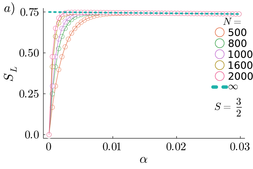
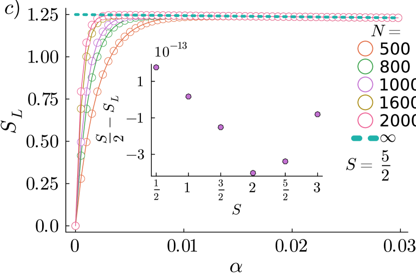
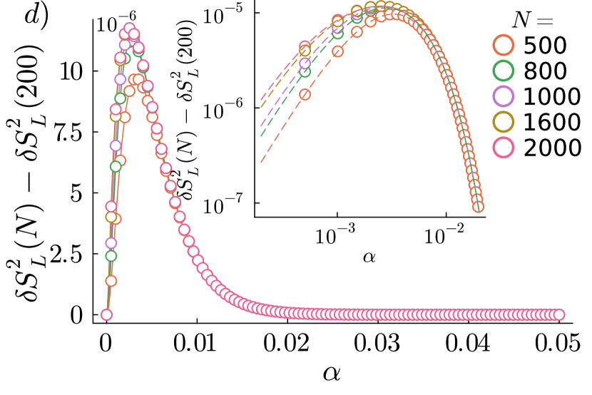
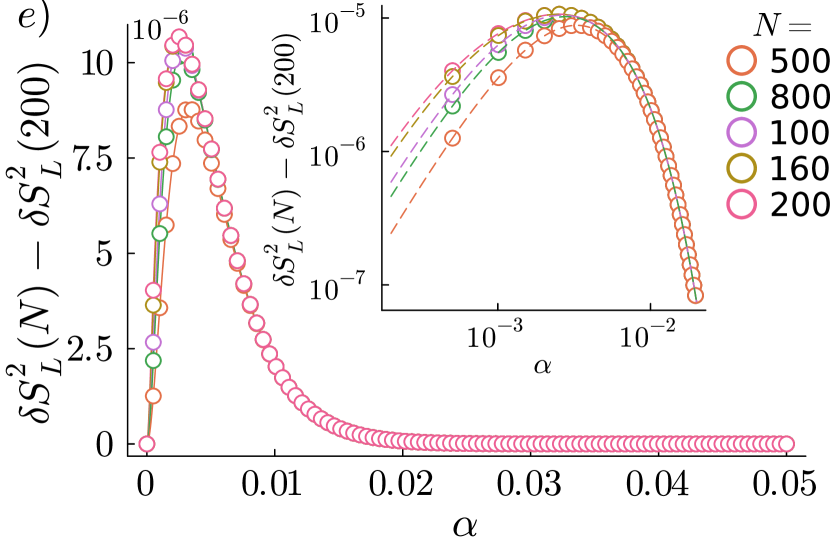
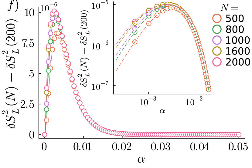
Figure 2: Spin accumulation and variance up to $S=3$: The finite size scaling of the left localized a) $\frac{3}{4}$ spin for $S=\frac{3}{2}$ and $\Delta=2$ $XXZ$ chain b) $1$ spin for $S=2$ and $\Delta=2$ $XXZ$ chain. The middle inset shows the DMRG result for $S\leq 3$ and extrapolation to higher spin by fitting the data c) $\frac{5}{4}$ spin for $S=\frac{5}{2}$ and $\Delta=2$ $XXZ$ chain. The right inset shows the difference between the expected outcome $\frac{S}{2}$ and DMRG result. The result is within the accuracy of the DMRG calculation. d) The variance of the edge spin operators $\delta S^{2}_{L}(N,\alpha)$ as well as their fit with the ansatz in Eq. (10) are shown in d), e) and f) for the edge spins shown in a), b) and c)respectively. The insets shows the fit with the ansatz for small values of $\alpha$.

Following [66, 67, 57], the fractional spin operators are defined as

$$\hat{S}^{z}_{L} =\lim_{\alpha\to 0}\lim_{N\to\infty}\sum_{j=1}^{N}e^{-\alpha j}S^{z}_{j};$$ (7)

and $\hat{S}^{z}_{R}$ is defined similarly but instead with the decay factor $e^{-\alpha(N+1-j)}$. Notice that in Eq. (7), the double limits are not interchangeable; The $N\to\infty$ limit has to be taken before taking $\alpha\to 0$ otherwise these equations give the total spin $S^{z}$ rather than the fractional edge spin. Numerically, it is often easier to compute $\hat{S}^{z}_{L/R}$ by plugging in Eq. (4) in Eq. (7) and using $\lim_{\alpha\to 0}(-1)^{j}e^{-\alpha j}=1/2$ results in the fractional spin being equal to the sum of the half chain spin profile and half of the bulk antiferromagnetic order[57].

Since it is difficult to take the thermodynamic limit $N\to\infty$ before taking $\alpha\to 0$ to evaluate Eq. (7) numerically, we determine its functional form through fitting that allows the limits to be taken after computing them for several values of $N$, $S$ and $\Delta$. We also computed the variance of the edge spin operators to validate the precise nature of the fractional spins identified thus far as sharp quantum observables. We define the spin variance for a finite size chain with sites $N$ as

$$\delta S^{2}_{L/R}(N,\alpha)=\braket{\hat{S}^{z}_{L/R}(N,\alpha)^{2}}-\braket{S^{z}_{L/R}(N,\alpha)}^{2}$$ (8)

where the average are taken in the ground state. Then, the variance defined in thermodynamic limit in Eq. (6) is obtained as

$$\delta S^{2}_{L/R}=\lim_{\alpha\to 0}\lim_{N\to\infty}\delta S^{2}_{L/R}(N,\alpha)$$ (9)

As mentioned earlier, taking the $N\to\infty$ limit numerically is a challenge which we circumvent by using the method introduced in [57] assuming that the variance at thermodynamic limit is related to the variance for finite size $N$ via

$$\delta S^{2}_{L/R}(N,\alpha)=\delta S^{2}_{L/R}(\infty,\alpha)-A\alpha e^{-B\alpha N}.$$ (10)

With the help of this ansatz, we can compute the variance in the thermodynamic limit as $\delta S^{2}_{L/R}=\lim_{\alpha\to 0}\delta S^{2}_{L/R}(\infty,\alpha)$. We verified the ansatz for various values of $N$ for Hamiltonian Eq. (1) as shown in the representative cases in Fig. 2 as it fits the data quite well.

We now compute the edge spin accumulation and the variance of the operators for Hamiltonian Eq. (1) for $S=\{\frac{1}{2},1,\frac{3}{2},2,\frac{5}{2},3\}$ and show that the fractional spin of magnitude $\frac{S}{2}$ exist in the edges and the variance of the spin operators vanish in each of these cases. The magnitude of localized edge modes for these cases are shown in Fig.2 and more plots for individual $S$ values are shown in the supplementary materials. In addition, more cases of perturbations that respect the three conditions and hence possessing the sharply localized edge modes are shown in the supplementary materials.

Breaking U(1) symmetry: To complete the argument we present some cases where the conditions outlined above are not satisfied. Consider the transverse field Ising model

$$H_{\mathrm{TFI}}=\sum_{i=1}^{N-1}\sigma_{i}^{z}\sigma_{i+1}^{z}+g\sum_{i=1}^{N}\sigma_{i}^{x}$$ (11)

in the antiferromagnetic phase. Since there is no $U(1)$ conservation, the criteria is violated. In such case, the spin accumulation is not quantized and the variance of the edge spin operators do not vanish as shown in Fig.3 for the representative case of $g=0.75$ for the spin accumulation in the left edge. A similar situation occurs in the XYZ model

$$H_{\mathrm{XYZ}}=\sum_{i=1}^{N-1}J_{x}S^{x}_{i}S^{x}_{i+1}+J_{y}S^{y}_{i}S^{y}_{i+1}+J_{z}S^{z}_{i}S^{z}_{i+1}$$ (12)

as shown in bottom panel of Fig.3 that as soon as the $U(1)$ symmetry is broken, the variance of the edge spin operator ceases to vanish. Let us start from the $XXZ-1$ with the couplings $J_{x}=J_{y}=1$ and $J_{z}=1.5$ where the edge spin is quantized to $\pm\frac{1}{2}$ and the variance of the edge spin vanishes. Now, we break the $U(1)$ symmetry by choosing the couplings $J_{x}=1,J_{y}=0.85$ and $J_{z}=1.5$. In this case, the variance of the edge spin operators do not vanish as shown in Fig.3. This shows that the $U(1)$ symmetry associated with the conservation of the $z-$component of the spin is essential for the existence of the robust edge spin. A detailed understanding of this effect we leave for future work.

Breaking Translational Symmetry: We break the translational symmetry in the system by adding disorder of the form $H_{D}=\sum_{j}(-1)^{j}W_{j}S^{z}_{j}$, where $W_{j}$ are random positive fields uniformly chosen from $[0,W]$, and the full Hamiltonian is now $H=H_{\Delta}+H_{D}$. This form of the disorder is chosen because it preserves the antiferromagnetic order in the bulk on average thereby satisfying all of our three criteria. We find that the edge mode is robust to this kind of disorder where not only the edge mode is quantized to $\pm\frac{S}{2}$ but also the variance of the edge spin operator vanishes in the thermodynamic limit. The effects of gap closing disorder are left for future work as they are more subtle because it induces spinon exciations in the bulk and its unclear, at present, how to analyze their contribution to the variance.

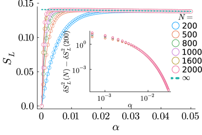
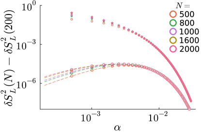
Figure 3: Breaking U(1) symmetry: The left panel shows that edge spin accumulation in the antiferromagnetic regime of transverse field Ising mode is not quantized to $\frac{S}{2}$. The inset shows that the variance of the edge spin operator does not vanish in the thermodynamic limit. The right figure shows that the variance of the left edge spin operator the spin-1 XYZ model (shown in circular marker) with couplings $J_{x}=1,J_{y}=0.85$ and $J_{z}=1.5$ does not vanish which is consistent with the fact that it does not satisfy the three conditions (shown with star marker) and the vanishing variance of the left edge spin operator the spin-1 XXZ model with couplings $J_{x}=J_{y}=1$ and $J_{z}=1.5$. The variance is fitted with the ansatz Eq. (10) for the latter case.

In conclusion, we found that in the ground state of spin$-S$ spin chains in the gapped antiferromagnetic phase there are fractional spin operators at the edges with eigenvalues $\pm\frac{S}{2}$. We presented two models where this argument was demonstrated exactly and further verified our argument up to spin $S=3$ XXZ chains with DMRG. Extensions to SU(N) magnets and systems with discrete symmetries is left to future work.

Acknowledgement: We thank T. Giamarchi for very useful discussions. J.H.P. is partially supported by NSF Career Grant No. DMR- 1941569.

In this supplementary material, we provide additional data and detailed analysis to support our main findings on ‘Edge spin fractionalization in one-dimensional spin-$S$ quantum antiferromagnets’. First, we present additional DMRG results for larger values of spin $S$ and demonstrate the spin accumulation in two-fold degenerate ground states with a representative example in Sec.I. We then explore various perturbations to the $XXZ-S$ model that respect the three conditions outlined in the main text, showing that these perturbations result in quantized edge spin accumulation and that the variance of the edge spin operator vanishes. Finally, we offer detailed analytical computations of the edge spin accumulation for three different models: the XX-$\frac{1}{2}$ model with a staggered magnetic field using the free fermion technique in Sec.III, the XXZ-$\frac{1}{2}$ chain using the Bethe Ansatz in Sec.IV, and the integrable deformation of the XXZ-1 chain using the Bethe Ansatz in Sec.V.

I Edge spin accumulation

For completeness, we have plotted the fractional edge spin accumulation $\frac{S}{2}$ for $XXZ-S$ model with $\Delta=2$ for $S=\left\{\frac{1}{2},1,\frac{3}{2},2,\frac{5}{2},3\right\}$ in Fig.4. The inset shows the vanishing variance for each of these cases.

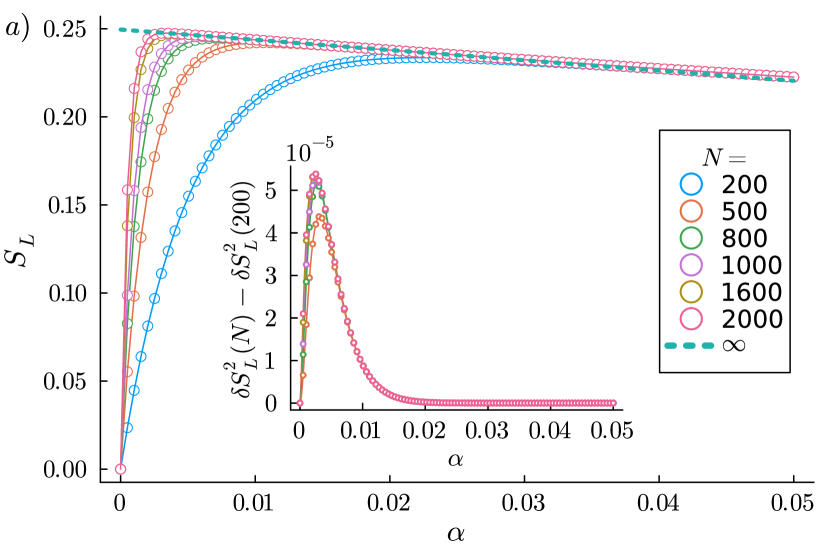
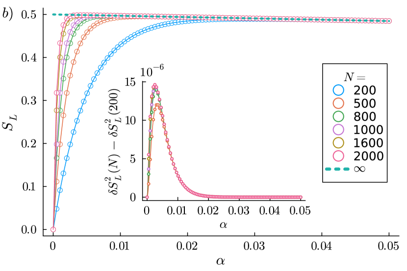
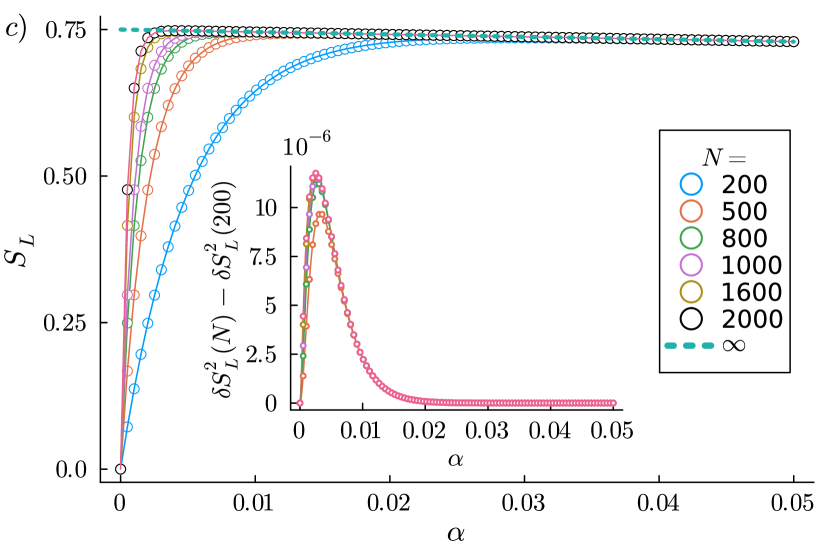
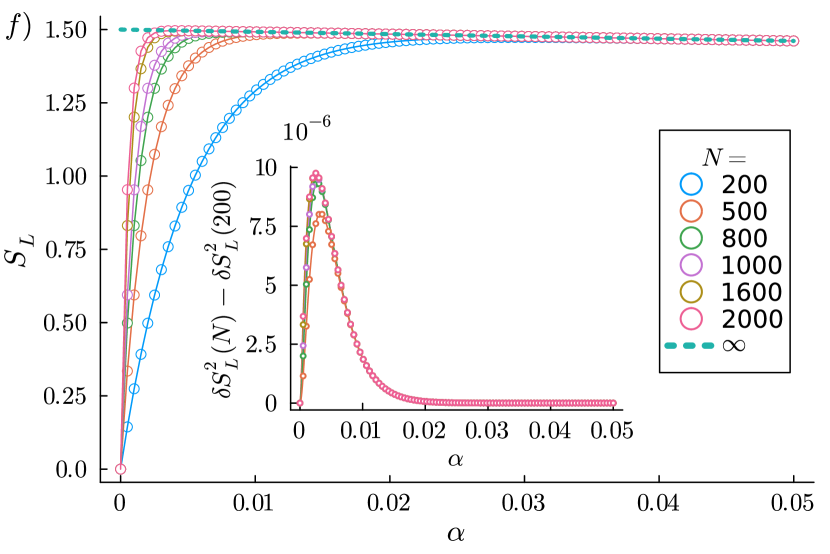
Figure 4: The fractionalized edge spin of magnitude $\frac{S}{2}$ for a) $S=\frac{1}{2}$, b) $S=1$, c) $S=\frac{3}{2}$, d) $S=2$, e) $S=\frac{5}{2}$ and f) $S=3$ and $\Delta=2$. The inset shows that ansatz for variance Eq. (10) fits the data very well. Thus, the variance vanishes for all of these cases in the thermodynamic limit thereby showing that edge spin is a well-defined quantum observable. Note that at the right edge there is $-\frac{S}{2}$ edge spin accumulation (not shown in the figures).

Notice that the $XXZ-S$ model for $\Delta>\Delta_{c_{2}}$ has spontaneous symmetry breaking which implies that there are two degenerate ground states. As claimed in the main text, for the odd total number of sites, the edge spin is of the form $\left|\frac{S}{2},\frac{S}{2}\right\rangle$ and $\left|-\frac{S}{2},-\frac{S}{2}\right\rangle$. We show the representative case for $S=1$ and $\Delta=2$ in Fig.5.

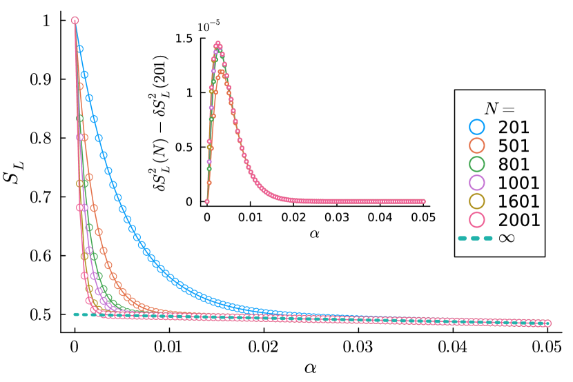
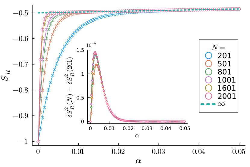
Figure 5: Left and right spin accumulation in the two degenerate ground state for $XXZ-1$ chain with $\Delta=2$ and odd number of sites. The inset shows that the variance fits well with the ansatz introduced in Eq. (10).

Moreover, we show that for some perturbation respecting the three conditions, the edge mode remains robust. As example cases of the perturbation that satisfy the three conditions, we consider the biquadratic deformation

$$H_{B}=\sum_{i=1}^{N-1}\cos(\theta)(\vec{S}_{i}\cdot\vec{S}_{i+1})_{\Delta}+\sin(\theta)\left(\vec{S}_{i}\cdot\vec{S}_{i+1}\right)^{2},$$ (1)

a perturbation by a uniform staggered magnetic field given by

$$H_{h}=\sum_{i=1}^{N-1}(\vec{S}_{i}\cdot\vec{S}_{i+1})_{\Delta}+\sum_{i=1}^{N}h(-1)^{i}S^{z}_{i},$$ (2)

a perturbation by a single-ion anisotropy term

$$H_{D}=\sum_{i=1}^{N-1}(\vec{S}_{i}\cdot\vec{S}_{i+1})_{\Delta}+D\sum_{i=1}^{N}(S^{z}_{i})^{2},$$ (3)

and a perturbation by next-near neighbor interaction

$$H_{J_{1}J_{2}}=J_{1}\sum_{i=1}^{N-1}(\vec{S}_{i}\cdot\vec{S}_{i+1})_{\Delta}-J_{2}\sum_{i=1}^{N-2}(\vec{S}_{i}\cdot\vec{S}_{i+2})_{\Delta}^{\prime},$$ (4)

in the antiferromagnetic regimes and show that the edge modes exist and the variance of the edge spin operator vanishes for representative cases in Fig.6.

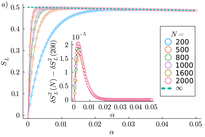
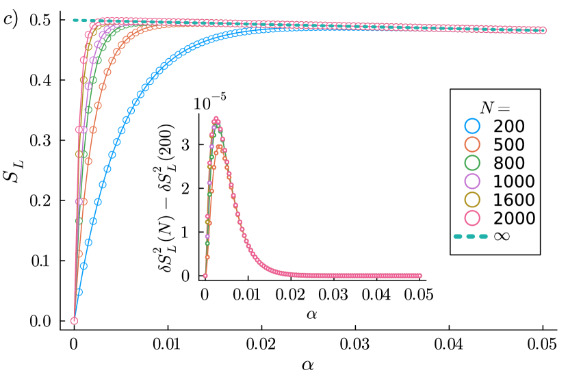
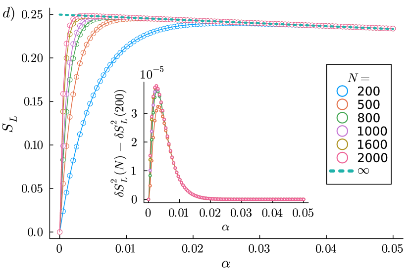
Figure 6: a) The fractional spin accumulation $\frac{1}{2}$ at the left end of the spin-1 anisotropic bilinear-biquadratic model for model Eq. (1) with parameter $\theta=\arctan\left(\frac{1}{3}\right)$ and $\Delta=1.5$. The inset shows the vanishing variance of the spin operator. b) The XXZ-$\frac{3}{2}$ chain with staggered magnetic field of magnitude $h=1.25$ at the isotropic point $\Delta=1$ given by Eq. (2) hosts $\frac{3}{4}$ fractional edge spin. As shown in the inset, the variance of the edge spin operator vanishes in the thermodynamic limit as it fits very well with the ansatz Eq. (10). c) The fractional spin accumulation of $\frac{1}{2}$ at the left edge of the XXZ-1 chain given by Eq. (3) with $\Delta=0.85$ and the single ion anisotropy $D=-1$. The inset shows the vanishing variance in the thermodynamic limit. d)The fractional spin accumulation of $\frac{1}{2}$ at the left edge of the XXZ-$\frac{1}{2}$ chain with next-near neighbor interaction given by Hamiltonian Eq. (4) with parameters $J_{1}=J_{2}=\Delta^{\prime}=1$ and $\Delta=1.75$. The inset shows the vanishing variance in the thermodynamic limit.

II Stability of the edge modes against weak disorder

As mentioned in the main text, the edge modes found in this work are stable against the weak disorder satisfying our three conditions.

In order to study the effect of disorder on the edge modes, we consider the Hamiltonian of the form

$$H=\sum_{i=1}^{N-1}S^{x}_{i}S^{x}_{i+1}+S^{y}_{i}S^{y}_{i+1}+\Delta S^{z}_{i}S^{z}_{i+1}+\sum_{j}(-1)^{j}W_{j}S^{z}_{j}$$ (5)

where $W_{j}$ are site dependent random positive magnetic fields. As shown in Fig.7 for the representative case of $S=\frac{1}{2}$ and $\Delta=2$, the edge modes are stable for weak disorder.

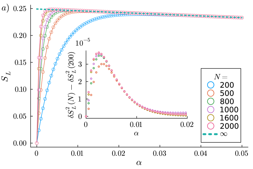
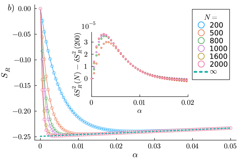
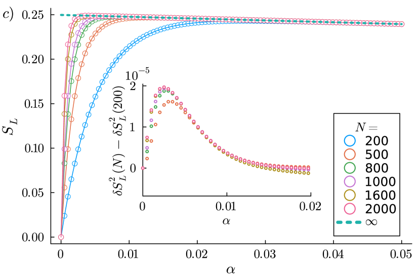
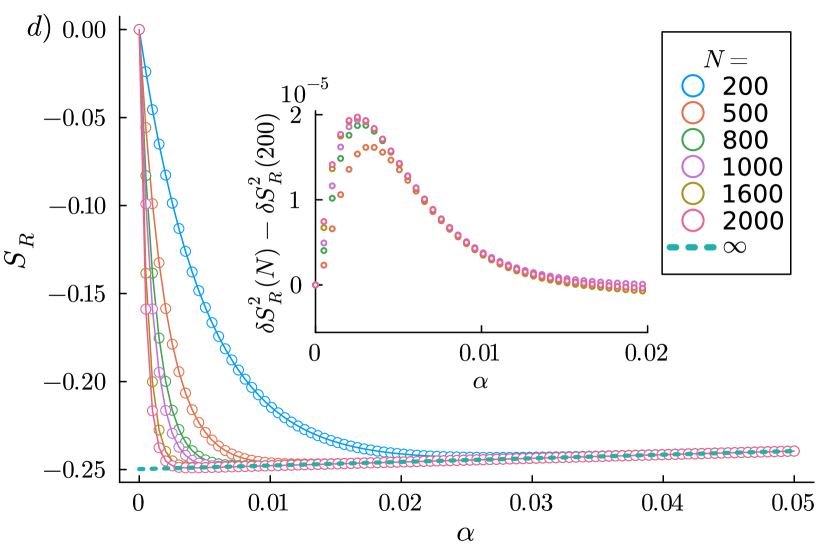
Figure 7: a) The left localized edge modes in the presence of weak disorder where each $W_{j}$ is randomly chosen from $[0,0.1]$ and $\Delta=2$. The data shown is averaged over 1000 samples. The inset shows that the variance vanishes in the thermodynamic limit. b) The right localized edge modes in the presence of weak disorder where each $W_{j}$ is randomly chosen from $[0,0.1]$ and $\Delta=2$. The inset shows that the variance vanishes in the thermodynamic limit. c) The left localized edge modes in the presence of disorder where each $W_{j}$ is randomly chosen from $[0,0.5]$ and $\Delta=2$. The inset shows that the variance vanishes in the thermodynamic limit. d) The right localized edge modes in the presence of disorder where each $W_{j}$ is randomly chosen from $[0,0.5]$ and $\Delta=2$. The inset shows that the variance vanishes in the thermodynamic limit.

III Free fermion case

Here, we construct a simple analytically tractable model with spin fractionalization which can be mapped to free Fermion via Jordon-Wigner transformation. The Hamiltonian under consideration is of the form:

$$H_{h}=\sum_{i=1}^{N-1}S^{x}_{i}S^{x}_{i+1}+S^{y}_{i}S^{y}_{i+1}+\sum_{i=1}^{N}h(-1)^{i}S^{z}$$ (6)

where $S^{i}$ are the spin matrices for the spin-$\frac{1}{2}$. Using Jordon-Wigner transformation, the Hamiltonian can be written as

$$H_{h}=\frac{1}{2}\left(\sum_{i=1}^{N-1}c_{i}^{\dagger}c_{i+1}+c_{i+1}^{\dagger}c_{i}\right)+\sum_{i=1}^{N}(-1)^{i}h(c_{i}^{\dagger}c_{i}-1/2)$$ (7)

When $h=0$ and $N$ is even, the normalized wafefunction is of the form

$$f_{n}(j)=\sqrt{\frac{2}{N+1}}\sum_{j}\sin\left(\frac{n\pi}{N+1}j\right)c_{j}^{\dagger}\ket{0}$$ (8)

and the eigenvalues are

$$E_{n}=\cos\left(k_{n}\right)$$ (9)

where $k_{n}=\frac{n\pi}{N+1}$ and $n=\{1,\cdots,N\}$

It is important to note that for $n=j$ and $n=N+1-j$, the energy eigenvalues are negative of each other and the amplitudes of the wavefunction are the same for these pairs.

The manybody ground state, thus, can be obtained by summing all the negative modes which corresponds to

$$E_{gs}=\sum_{n=\frac{N}{2}+1}^{N}\cos\left(\frac{n\pi}{N+1}\right)$$ (10)

Now, when $h\neq 0$, the eigenvalues are

$$E_{n}=\pm\sqrt{\cos^{2}(k)+h^{2}}$$ (11)

where $k=\frac{n^{\prime}\pi}{N+1}$ and $n^{\prime}=\{1,\cdots,{N}/{2}\}$

and the ground state is simply

$$E_{gs}(h)=-\sum_{n=1}^{\frac{N}{2}}\sqrt{h^{2}+\cos^{2}\left(\frac{n\pi}{N+1}\right)}$$ (12)

Now, we focus on the positive parity solutions, with eigen state

$$E_{n}=\sqrt{h^{2}+\cos^{2}\left(\frac{n\pi}{N+1}\right)}$$ (13)

whose corresponding normalized wavefunction, is

$$\psi_{n}(j)=\frac{1}{\sqrt{1+\left(\frac{h}{\cos(\frac{n\pi}{N+1})+\sqrt{h^{2}+\cos^{2}\left(\frac{n\pi}{N+1}\right)}}\right)^{2}}}\left(f_{n}(j)+\frac{h}{\cos(\frac{n\pi}{N+1})+\sqrt{h^{2}+\cos^{2}\left(\frac{n\pi}{N+1}\right)}}f_{N+1-n}(j)\right)$$ (14)

Notice, that $n$ runs from 1 to $N/2$ only. Thus, there are only half of the eigenvalues which corresponds to the positive parity solution.

Now, we consider the negative parity eigenvalues

$$E_{n}=-\sqrt{h^{2}+\cos^{2}\left(\frac{n\pi}{N+1}\right)}$$ (15)

Then, the eigenvalues are given by [68])

$$\chi_{n}(j)=\frac{1}{\sqrt{1+\left(\frac{\cos(\frac{n\pi}{N+1})+\sqrt{h^{2}+\cos^{2}\left(\frac{n\pi}{N+1}\right)}}{h}\right)^{2}}}\left(f_{n}(j)-\frac{\cos(\frac{n\pi}{N+1})+\sqrt{h^{2}+\cos^{2}\left(\frac{n\pi}{N+1}\right)}}{h}f_{N+1-n}(j)\right)$$ (16)

Again $n$ runs from 1 to $\frac{N}{2}$. Thus, there are only half of the solutions but there are precisely the one particle solutions that have negative energies! Thus, we have to use the $\chi$ solutions to do the ground state calculations!

The spin profile is simply given by

$$S^{z}_{j}=\left(\sum_{n=1}^{\frac{N}{2}}|\chi_{n}(j)|^{2}\right)-1/2$$ (17)

We can simplify Eq. (17) as

$$S^{z}_{j} =(-1)^{j}\sum_{n=1}^{\frac{N}{2}}\frac{2\sqrt{2}h\sin^{2}\left(\frac{\pi jn}{N+1}\right)}{(N+1)\sqrt{2h^{2}+\cos\left(\frac{2\pi n}{N+1}\right)+1}}$$

$$\stackrel{{\scriptstyle\lim_{N\to\infty}}}{{=}}(-1)^{j}\int_{0}^{\frac{1}{2}}\frac{2h\sin^{2}(\pi jx)}{\sqrt{h^{2}+\cos^{2}(\pi x)}}\,dx$$ (18)

Note that in the last step, we took $N\to\infty$ limit. Fortunately, this does not wash away the effect of the boundary in the left end. But indeed, it washes away the effect on the right boundary. However, if we recall $S^{z}_{j}=-S^{z}_{N+1-j}$ for even parity and $S^{z}_{j}=S^{z}_{N+1-1}$ for odd parity, we shall be able to construct the full profile of the chain.

It is now possible to find the bulk antiferromagnetic order as

$$\mathfrak{S}(h)=\int_{0}^{\frac{1}{2}}\frac{h}{\sqrt{h^{2}+\cos^{2}(\pi x)}}\mathrm{d}x=\frac{hK\left(\frac{1}{h^{2}+1}\right)}{\pi\sqrt{h^{2}+1}}$$ (19)

where $K$ is the complete elliptic integral of the first kind defined as

$$K(k)=\int_{0}^{\frac{\pi}{2}}\frac{d\theta}{\sqrt{1-k\cos^{2}\theta}}$$ (20)

Although, a closed form expression for Eq. (18) for generic $j$ seems difficult, it is not difficult to numerically observe that

$$\sum_{j=1}^{\frac{N}{2}}S^{z}_{j}-\frac{1}{2}\mathfrak{S}(h)=-\frac{1}{4}$$ (21)

irrespective of the value of $h$ for even $N$.

IV XXZ-1/2

The integrable spin-$\frac{1}{2}$ spin chain in the gapped antiferromagnetic phase is described by the Hamiltonian of the form

$$H_{\Delta}=\sum_{i=1}^{N-1}\frac{J}{2}(\sigma_{i}^{x}\otimes\sigma_{i+1}^{x}+\sigma_{i}^{y}\otimes\sigma_{i+1}^{y}+\Delta\sigma_{i}^{z}\otimes\sigma_{i+1}^{z})$$ (22)

which can be solved exactly by using Bethe Ansatz. The Bethe Ansatz equations are

$$\begin{gathered}\left(\frac{\sin\frac{1}{2}\left(\lambda_{j}-{i\eta}\right)}{\sin\frac{1}{2}\left(\lambda_{j}+{i\eta}\right)}\right)^{2N}\frac{\cos^{2}\frac{1}{2}\left(\lambda_{j}+{i\eta}\right)}{\cos^{2}\frac{1}{2}\left(\lambda_{j}-{i\eta}\right)}=\prod_{k=1(\neq j)}^{M}\frac{\sin\frac{1}{2}\left(\lambda_{j}-\lambda_{k}-2i\eta\right)\sin\frac{1}{2}\left(\lambda_{j}+\lambda_{k}-2i\eta\right)}{\sin\frac{1}{2}\left(\lambda_{j}-\lambda_{k}+2i\eta\right)\sin\frac{1}{2}\left(\lambda_{j}+\lambda_{k}+2i\eta\right)}\end{gathered}$$ (23)

where $\Delta=\cosh(\eta)$.

Taking $\log$ on both sides of Eq. (23), we write

$$(2N+1)\phi\left(\lambda_{j},\eta\right)-2\psi\left(\lambda_{j},\eta\right)+\psi(\lambda_{j},\eta)=\pi iI_{j}+\sum_{k}\left[\phi(\lambda_{j}+\lambda_{k},2\eta)+\phi(\lambda_{j}-\lambda_{k},2\eta)\right]$$ (24)

Where we introduced

$$\phi(a,b) =\log\left(\frac{\sin\frac{1}{2}(a-ib)}{\sin\frac{1}{2}(a+ib)}\right)$$ (25)

$$\psi(a,b) =\log\left(\frac{\cos\frac{1}{2}(a-ib)}{\cos\frac{1}{2}(a+ib)}\right)$$ (26)

We extract the density of roots in the ground state $\rho_{0}(\lambda)$ by subtracting Eq. (24) written for $\lambda_{j}$ from the same equation written for $\lambda_{j+1}$ and expanding in the difference $\Delta\lambda=\lambda_{j+1}-\lambda_{j}$. This gives

$$(2N+1) a(\lambda,\eta)-2a\left(\lambda-\pi,\eta\right)+a(\lambda-\pi,\eta)$$

$$=2\pi\rho(\lambda)+\int\rho(\lambda)\left[a(\lambda-\lambda^{\prime},2\eta)+a(\lambda+\lambda^{\prime},2\eta)\right]\mathrm{d}\lambda^{\prime}+2\pi\delta(\lambda)+2\pi\delta(\lambda-\pi),$$ (27)

where we introduced

$$a(x,y)=\frac{\sinh(y)}{\cosh(y)-\cos(x)}$$ (28)

and we added delta function at $\lambda=0$ and $\lambda=\pi$ to remove the two solutions which lead to vanishing wavefunction.

Using the following convention for Fourier transform

$$f(x)=\sum_{\omega=-\infty}^{\infty}\hat{f}(\omega)e^{i\omega x}\quad\quad\text{and}\quad\quad\hat{f}(\omega)=\frac{1}{2\pi}\int_{-\pi}^{\pi}f(x)e^{-i\omega x}dx,$$ (29)

we compute

$$\hat{a}(\omega,y)=\frac{1}{2\pi}\int_{-\pi}^{\pi}e^{-i\omega x}\sum_{k=-\infty}^{\infty}e^{ikx}\left(e^{-y}\right)^{|k|}=e^{-y|\omega|}$$ (30)

Now the solution of Eq. (27) is immediate in the Fourier space

$$\tilde{\rho}_{\ket{\frac{1}{2}}}(\omega)=\frac{(2N+1)e^{-\eta|\omega|}+(-1)^{\omega}e^{-\eta|\omega|}-2(-1)^{\omega}e^{-\eta|\omega|}-(1+(-1)^{\omega})}{4\pi(1+e^{-2\eta|\omega|})}$$ (31)

The total number of Bethe roots is given by

$$M_{\ket{\frac{1}{2}}}=\int_{-\pi}^{\pi}\rho_{\ket{\frac{1}{2}}}(\lambda)\mathrm{d}\lambda=2\pi\tilde{\rho}_{\ket{\frac{1}{2}}}(0)=\frac{N-1}{2}$$ (32)

Since the total number of Bethe roots is not an integer when $N$ is even.

However, if we were to treat it as a valid state and compute it’s spin, we find

$$S^{z}_{\ket{\frac{1}{2}}}=\frac{N}{2}-M_{\ket{\frac{1}{2}}}=\frac{1}{2}$$ (33)

It will be important later to understand the spin configuration of this configuration of the Bethe roots. The $\frac{1}{2}$ here comes from the two boundary terms equally contributing to this spin accumulation. Due to the gap in the bulk, this spin configuration has to be $\frac{1}{4}$ in each end of the chain. Moreover, because of the $SU(2)$ symmetry there is also configuration with spin $\pm\frac{1}{2}$ where each end has $\pm\frac{1}{4}$ sharply localized spin as shown in Fig.8.

Figure 8: Schematic of the edge localized spin quarter spin

To get the actual ground state We need to add the complex solution $\lambda_{bs}=\pi\pm i\eta$. Adding the complex solution $\lambda_{bs}$, we the Bethe equation becomes

$$\left(\frac{\sin\frac{1}{2}\left(\lambda_{j}-{i\eta}\right)}{\sin\frac{1}{2}\left(\lambda_{j}+{i\eta}\right)}\right)^{2N}\frac{\cos^{2}\frac{1}{2}\left(\lambda_{j}+{i\eta}\right)}{\cos^{2}\frac{1}{2}\left(\lambda_{j}-{i\eta}\right)}$$ (34)

$$=\prod_{k=1(\neq j)}^{M}\frac{\sin\frac{1}{2}\left(\lambda_{j}-\lambda_{k}-2i\eta\right)\sin\frac{1}{2}\left(\lambda_{j}+\lambda_{k}-2i\eta\right)}{\sin\frac{1}{2}\left(\lambda_{j}-\lambda_{k}+2i\eta\right)\sin\frac{1}{2}\left(\lambda_{j}+\lambda_{k}+2i\eta\right)}\frac{\cos\left(\frac{1}{2}\left(\lambda_{j}-i\eta\right)\right)\cos\left(\frac{1}{2}\left(\lambda_{j}-3i\eta\right)\right)}{\cos\left(\frac{1}{2}\left(\lambda_{j}+i\eta\right)\right)\cos\left(\frac{1}{2}\left(\lambda_{j}+3i\eta\right)\right)}$$ (35)

Taking $log$ on both sides of the equation, we obtain

$$(2N+1) \phi\left(\lambda_{j},\eta\right)-2\psi\left(\lambda_{j},\eta\right)$$

$$+\psi(\lambda_{j},\eta)=2\pi iI_{j}+\sum_{k}\left[\phi(\lambda_{j}+\lambda_{k},2\eta)+\phi(\lambda_{j}-\lambda_{k},2\eta)\right]+\psi(\lambda_{j},\eta)+\psi(\lambda_{j},3\eta)$$ (36)

Differentiating and removing $\lambda=0$ and $\lambda=\pi$ solution, we get

$$(2N+1)a(\lambda,\eta)-2a\left(\lambda-\pi,\eta\right)+a(\lambda-\pi,\eta)-2\pi\delta(\lambda)-2\pi\delta(\lambda-\pi$$

$$=2\pi\rho(\lambda)+\int\rho(\lambda)\left[a(\lambda-\lambda^{\prime},2\eta)+a(\lambda+\lambda^{\prime},2\eta)\right]\mathrm{d}\lambda^{\prime}+a(\lambda-\pi,\eta)+a(\lambda-\pi,3\eta))$$ (37)

solving for the solution density in Fourier space we obtain

$$\tilde{\rho}_{\ket{0}_{bs}}(\omega)=\frac{(2N+1)e^{-\eta|\omega|}+(-1)^{\omega}e^{-\eta|\omega|}-2(-1)^{\omega}e^{-\eta|\omega|}-(1+(-1)^{\omega})}{4\pi(1+e^{-2\eta|\omega|})}-\frac{(-1)^{\omega}}{4\pi}\frac{e^{-\eta|\omega|}+e^{-3\eta|\omega|}}{(1+e^{-2\eta|\omega|})}$$ (38)

The total number of Bethe roots is given by

$$M_{{\ket{0}_{bs}}}=1+\int_{-\pi}^{\pi}\rho_{\ket{0}}(\lambda)\mathrm{d}\lambda=1+2\pi\tilde{\rho}_{\ket{0}}(0)=\frac{N}{2}$$ (39)

Thus, the total spin is equal to

$$S^{z}_{{\ket{0}_{bs}}}=\frac{N}{2}-M_{{\ket{0}_{bs}}}=0$$ (40)

Which shows that the only logical way to explain it is that the two quarter spin localized at the edges in the root configuration described by Eq. (33) became $\frac{1}{4}$ at one end at $-\frac{1}{4}$ quarter at another end because the spin weight of the boundary string is $-\frac{1}{2}$. This is a natural interpretation because the bulk $2-$ string solution makes the two holes in triplet configuration to singlet pair. Hence, we expect that the boundary string solution makes two two edge modes into a singlet. Thus, the two fold degenerate ground state has the spin configuration where quarter edge modes are pointed in opposite direction as shown in figure Fig.9.

Figure 9: Cartoon depicting exponentially localized quarter spin in the ground state of XXZ-$\frac{1}{2}$ spin chain.

Recall that the bulk is gapped and hence the correlation in the model fall exponentially. Thus, any perturbation in the bulk which does not close the gap and change the symmetry can not change this edge physics. This is what we established numerically in the main text.

V Integrable spin-1 chain

Spin-$1$ XXZ chain is made up of two copies of spin-$\frac{1}{2}$ spin chain fused together. First consider the integrable Hamiltonian

$$H_{1}=\sum_{n}\sigma_{n}-(\sigma_{n})^{2}+2\sinh^{2}(\eta)\left[\sigma^{z}_{n}+(S^{z}_{n})^{2}+(S^{z}_{n+1})^{2}-(\sigma^{z}_{n})^{2}\right]-4\sinh^{2}\left(\frac{\eta}{2}\right)(\sigma^{\perp}_{n}\sigma^{z}_{n}+\sigma^{z}_{n}\sigma^{\perp}_{n})$$ (41)

Where:

$$\sigma_{n} =\vec{S}_{n}\cdot\vec{S}_{n+1}$$

$$\sigma^{\perp}_{n} =S^{x}_{n}S^{x}_{n+1}+S^{y}_{n}S^{y}_{n+1}$$

$$\sigma^{z}_{n} =S^{z}_{n}S^{z}_{n+1}$$

and $S_{n}^{i}$ for $i=\{x,y,z\}$ are the spin-1 represetation of $SU(2)$.

We can write the model as

$$H_{1}=H_{\Delta}+H^{I}$$ (42)

where

$$H_{\Delta}=\sum_{n}S^{x}_{n}S^{x}_{n+1}+S^{y}_{n}S^{y}_{n+1}+\Delta S^{z}_{n}S^{z}_{n+1},$$ (43)

with $\Delta=1+2\sinh^{2}\eta$ and the integrable deformation terms

$$H^{I}=\sum_{i}2\sinh^{2}(\eta)\left[(S^{z}_{n})^{2}+(S^{z}_{n+1})^{2}-(\sigma^{z}_{n})^{2}\right]-4\sinh^{2}\left(\frac{\eta}{2}\right)(\sigma^{\perp}_{n}\sigma^{z}_{n}+\sigma^{z}_{n}\sigma^{\perp}_{n})-(\sigma_{n})^{2}.$$ (44)

Using the fusion method described elsewhere [61, 62, 63], we obtain the BAE for spin-1 case

$$\begin{gathered}\left(\frac{\sin\frac{1}{2}\left(\lambda_{j}-{2i\eta}\right)}{\sin\frac{1}{2}\left(\lambda_{j}+{2i\eta}\right)}\right)^{2N}\frac{\cos^{2}\frac{1}{2}\left(\lambda_{j}+{2i\eta}\right)}{\cos^{2}\frac{1}{2}\left(\lambda_{j}-{2i\eta}\right)}=\prod_{k=1(\neq j)}^{M}\frac{\sin\frac{1}{2}\left(\lambda_{j}-\lambda_{k}-2i\eta\right)\sin\frac{1}{2}\left(\lambda_{j}+\lambda_{k}-2i\eta\right)}{\sin\frac{1}{2}\left(\lambda_{j}-\lambda_{k}+2i\eta\right)\sin\frac{1}{2}\left(\lambda_{j}+\lambda_{k}+2i\eta\right)}\end{gathered}$$ (45)

The ground state of spin-S chain is given by a vacuum of 2S string solution, thus, putting $\lambda_{j}\to\chi_{j}\pm i\eta$, we obtain

$$\left(\frac{\sin\left(\frac{1}{2}\left(\chi_{j}-3i\eta\right)\right)}{\sin\left(\frac{1}{2}\left(\chi_{j}+3i\eta\right)\right)}\right)^{2N}\left(\frac{\sin\left(\frac{1}{2}\left(\chi_{j}-i\eta\right)\right)}{\sin\left(\frac{1}{2}\left(\chi_{j}+i\eta\right)\right)}\right)^{2N}\left(\frac{\cos\left(\frac{1}{2}\left(\chi_{j}+3i\eta\right)\right)}{\cos\left(\frac{1}{2}\left(\chi_{j}-3i\eta\right)\right)}\right)^{2}\left(\frac{\cos\left(\frac{1}{2}\left(\chi_{j}+i\eta\right)\right)}{\cos\left(\frac{1}{2}\left(\chi_{j}-i\eta\right)\right)}\right)^{2}$$

$$\frac{\sin\left(\chi_{j}-i\eta\right)}{\sin\left(\chi_{j}+i\eta\right)}=\prod_{k=1}^{M}\frac{\sin\left(\frac{1}{2}\left(\chi_{j}-\chi_{k}-4i\eta\right)\right)}{\sin\left(\frac{1}{2}\left(\chi_{j}-\chi_{k}+4i\eta\right)\right)}\left(\frac{\sinh\left(\frac{1}{2}\left(\chi_{j}-\chi_{k}-2i\eta\right)\right)}{\sinh\left(\frac{1}{2}\left(\chi_{j}-\chi_{k}+2i\eta\right)\right)}\right)^{2}\times$$

$$\hskip 142.26378pt\frac{\sin\left(\frac{1}{2}\left(\chi_{j}+\chi_{k}-4i\eta\right)\right)}{\sin\left(\frac{1}{2}\left(\chi_{j}+\chi_{k}+4i\eta\right)\right)}\left(\frac{\sinh\left(\frac{1}{2}\left(\chi_{j}+\chi_{k}-2i\eta\right)\right)}{\sinh\left(\frac{1}{2}\left(\chi_{j}+\chi_{k}+2i\eta\right)\right)}\right)^{2}$$ (46)

Writing,

$$\frac{\sin\left(\chi_{j}-i\eta\right)}{\sin\left(\chi_{j}+i\eta\right)}=\frac{\sin\left(\frac{1}{2}\left(\chi_{j}-i\eta\right)\right)\cos\left(\frac{1}{2}\left(\chi_{j}-i\eta\right)\right)}{\sin\left(\frac{1}{2}\left(\chi_{j}+i\eta\right)\right)\cos\left(\frac{1}{2}\left(\chi_{j}+i\eta\right)\right)},$$ (47)

we rewrite the Bethe equations in the convenient logarithmic form as

$$(2N+1)\phi\left(\chi_{j},\eta\right)+2N\phi(\chi_{j},3\eta)-2\psi\left(\chi_{j},\eta\right)-2\psi(\chi_{j},3\eta)+\psi(\chi_{j},\eta)$$

$$=\pi iI_{j}+\sum_{k}\left[\phi(\chi_{j}+\chi_{k},4\eta)+\phi(\chi_{j}-\chi_{k},4\eta)+2\phi(\chi_{j}-\chi_{k},2\eta)+2\phi(\chi_{j}+\chi_{k},2\eta)\right]$$ (48)

Where we introduced

$$\phi(a,b) =\log\left(\frac{\sin\frac{1}{2}(a-ib)}{\sin\frac{1}{2}(a+ib)}\right)$$ (49)

$$\psi(a,b) =\log\left(\frac{\cos\frac{1}{2}(a-ib)}{\cos\frac{1}{2}(a+ib)}\right)$$ (50)

We extract the density of roots in the ground state $\rho_{0}(\lambda)$ by subtracting Eq. (48) written for $\lambda_{j}$ from the same equation written for $\lambda_{j+1}$ and expanding in the difference $\Delta\lambda=\lambda_{j+1}-\lambda_{j}$. This gives

$$(2N+1) a(\chi,\eta)+2Na(\chi,3\eta)-2a\left(\chi-\pi,\eta\right)-2a\left(\chi-\pi,3\eta\right)+a(\lambda-\pi,\eta)$$

$$=2\pi\rho(\lambda)+\int\rho(\lambda)\left[a(\lambda-\lambda^{\prime},4\eta)+a(\lambda+\lambda^{\prime},4\eta)+2a(\lambda-\lambda^{\prime},2\eta)+2a(\lambda+\lambda^{\prime},2\eta)\right]\mathrm{d}\lambda^{\prime}$$

$$+4\pi\delta(\lambda)+4\pi\delta(\lambda-\pi),$$ (51)

where we introduced

$$a(x,y)=\frac{\sinh(y)}{\cosh(y)-\cos(x)}$$ (52)

and we added delta function at $\lambda=0$ and $\lambda=\pi$ to remove the two solutions which lead to vanishing wavefunction.

Using the following convention for Fourier transform

$$f(x)=\sum_{\omega=-\infty}^{\infty}\hat{f}(\omega)e^{i\omega x}\quad\quad\text{and}\quad\quad\hat{f}(\omega)=\frac{1}{2\pi}\int_{-\pi}^{\pi}f(x)e^{-i\omega x}dx,$$ (53)

we compute

$$\hat{a}(\omega,y)=\frac{1}{2\pi}\int_{-\pi}^{\pi}e^{-i\omega x}\sum_{k=-\infty}^{\infty}e^{ikx}\left(e^{-y}\right)^{|k|}=e^{-y|\omega|}$$ (54)

Now the solution of Eq. (51) is immediate in the Fourier space

$$\tilde{\rho}_{\ket{1}}(\omega)=\frac{(2N+1)e^{-\eta|\omega|}+2Ne^{-3\eta|\omega|}+(-1)^{\omega}e^{-\eta|\omega|}-2(-1)^{\omega}e^{-\eta|\omega|}-2(-1)^{\omega}e^{-3\eta|\omega|}-(1+(-1)^{\omega})}{4\pi(1+e^{-4\eta|\omega|}+2e^{2\eta|\omega|})}$$ (55)

The total number of center of roots is given by

$$M_{\ket{1}}=\int_{-\pi}^{\pi}\rho_{\ket{\frac{1}{2}}}(\lambda)\mathrm{d}\lambda=2\pi\tilde{\rho}_{\ket{\frac{1}{2}}}(0)=\frac{N-1}{2}$$ (56)

However, this is not possible for even $N$. If this were a valid state, the spin of this state would be

$$N-2M=1$$ (57)

Once again due to the $SU(2)$ symmetry, there is also configuration with same Bethe roots with spin $-1$. These state are not valid state as the number of centers of the root is not integer. But, it is important to look at the spin configuration of these roots distribution which are exponentially localized $\frac{1}{2}$ spin at the two edges just as like in spin-$\frac{1}{2}$ case.

Now, to construct a valid ground state state, we need to add the boundary string. Adding the boundary string $\pi\pm 2i\eta$ the list of the solution in Eq. (45), we obtain the equation for ground state as

$$\left(\frac{\sin\left(\frac{1}{2}\left(\chi_{j}-3i\eta\right)\right)}{\sin\left(\frac{1}{2}\left(\chi_{j}+3i\eta\right)\right)}\right)^{2N} \left(\frac{\sin\left(\frac{1}{2}\left(\chi_{j}-i\eta\right)\right)}{\sin\left(\frac{1}{2}\left(\chi_{j}+i\eta\right)\right)}\right)^{2N}\left(\frac{\cos\left(\frac{1}{2}\left(\chi_{j}+3i\eta\right)\right)}{\cos\left(\frac{1}{2}\left(\chi_{j}-3i\eta\right)\right)}\right)^{2}\left(\frac{\cos\left(\frac{1}{2}\left(\chi_{j}+i\eta\right)\right)}{\cos\left(\frac{1}{2}\left(\chi_{j}-i\eta\right)\right)}\right)^{2}$$

$$\frac{\sin\left(\frac{1}{2}\left(\chi_{j}-i\eta\right)\right)\cos\left(\frac{1}{2}\left(\chi_{j}-i\eta\right)\right)}{\sin\left(\frac{1}{2}\left(\chi_{j}+i\eta\right)\right)\cos\left(\frac{1}{2}\left(\chi_{j}+i\eta\right)\right)} =\left(\frac{\cos\left(\frac{1}{2}\left(\chi_{j}-5i\eta\right)\right)}{\cos\left(\frac{1}{2}\left(\chi_{j}+5i\eta\right)\right)}\right)^{2}\left(\frac{\cos\left(\frac{1}{2}\left(\chi_{j}-3i\eta\right)\right)}{\cos\left(\frac{1}{2}\left(\chi_{j}+3i\eta\right)\right)}\right)^{2}$$

$$\prod_{k=1}^{M}\frac{\sin\left(\frac{1}{2}\left(\chi_{j}-\chi_{k}-4i\eta\right)\right)}{\sin\left(\frac{1}{2}\left(\chi_{j}-\chi_{k}+4i\eta\right)\right)}\left(\frac{\sinh\left(\frac{1}{2}\left(\chi_{j}-\chi_{k}-2i\eta\right)\right)}{\sinh\left(\frac{1}{2}\left(\chi_{j}-\chi_{k}+2i\eta\right)\right)}\right)^{2}\times$$

$$\frac{\sin\left(\frac{1}{2}\left(\chi_{j}+\chi_{k}-4i\eta\right)\right)}{\sin\left(\frac{1}{2}\left(\chi_{j}+\chi_{k}+4i\eta\right)\right)}\left(\frac{\sinh\left(\frac{1}{2}\left(\chi_{j}+\chi_{k}-2i\eta\right)\right)}{\sinh\left(\frac{1}{2}\left(\chi_{j}+\chi_{k}+2i\eta\right)\right)}\right)^{2}$$ (58)

Such that the solution for the root density is immediate in the Fourier space

$$\tilde{\rho}_{\ket{0}}(\omega) =\frac{(2N+1)e^{-\eta|\omega|}+2Ne^{-3\eta|\omega|}+(-1)^{\omega}e^{-\eta|\omega|}-2(-1)^{\omega}e^{-\eta|\omega|}-2(-1)^{\omega}e^{-3\eta|\omega|}-(1+(-1)^{\omega})}{4\pi(1+e^{-4\eta|\omega|}+2e^{2\eta|\omega|})}$$

$$-\frac{2(-1)^{\omega}e^{-5\eta|\omega|}+2(-1)^{\omega}e^{-3\eta|\omega|}}{{4\pi(1+e^{-4\eta|\omega|}+2e^{2\eta|\omega|})}}$$ (59)

The total number of center of bulk roots is given by

$$M_{\ket{0}}=\int_{-\pi}^{\pi}\rho_{\ket{0}}(\lambda)\mathrm{d}\lambda=2\pi\tilde{\rho}_{\ket{0}}(0)=\frac{N-2}{2}$$ (60)

And the total spin is given by

$$S^{z}=N-2\left(1+\frac{N-2}{2}\right)=0$$ (61)

The spin configuration is now made up of fractionalized spin$-\frac{1}{2}$ localized at the edges which point in opposite direction just like in the spin-$\frac{1}{2}$ as depicted in the fig.9 but with maginitude $\pm\frac{1}{2}$.

We showed that $\pm\frac{1}{2}$ spin is localized at the edge of this fine tuned model. However, it is important to understand that any perturbations that do not close the gap and change the symmetry can change the boundary physics. Thus, we expect the regular XXZ-1 spin chain with Hamiltonian

$$H_{\Delta}=\sum_{i=1}^{N=1}S^{x}_{i}S^{x}_{i+1}+S^{y}_{i}S^{y}_{i+1}+\Delta S^{z}_{i}S^{z}_{i+1}$$ (62)

has to have this edge mode as long as $\Delta>\Delta_{c_{2}}$. We prove this claim numerically in the main text. Moreover, we also test by adding next near neighbor interaction or biquadratic term that as long as we are in the gapped antiferromagnetic regime, the edge modes exist as robust quantum observables.

References

• JackiwΒ andΒ Rebbi [1976] R.Β JackiwΒ andΒ C.Β Rebbi,Β Solitons with fermion number Β½,Β Phys. Rev. DΒ 13,Β 3398 (1976).
• SuΒ etΒ al. [1979] W.Β P.Β Su, J.Β R.Β Schrieffer,Β andΒ A.Β J.Β Heeger,Β Solitons in polyacetylene,Β Phys. Rev. Lett.Β 42,Β 1698 (1979).
• Giamarchi [2003] T.Β Giamarchi,Β Quantum physics in one dimension,Β Vol.Β 121Β (Clarendon press,Β 2003).
• TynerΒ andΒ Goswami [2023] A.Β C.Β TynerΒ andΒ P.Β Goswami,Β Spin-charge separation and quantum spin hall effect of $\beta$-bismuthene,Β Scientific reportsΒ 13,Β 11393 (2023).
• KaneΒ andΒ Mele [2005a] C.Β L.Β KaneΒ andΒ E.Β J.Β Mele,Β Z 2 topological order and the quantum spin hall effect,Β Physical review lettersΒ 95,Β 146802 (2005a).
• Balents [2010] L.Β Balents,Β Spin liquids in frustrated magnets,Β natureΒ 464,Β 199 (2010).
• BroholmΒ etΒ al. [2020] C.Β Broholm, R.Β Cava, S.Β Kivelson, D.Β Nocera, M.Β Norman,Β andΒ T.Β Senthil,Β Quantum spin liquids,Β ScienceΒ 367,Β eaay0668 (2020).
• SavaryΒ andΒ Balents [2016] L.Β SavaryΒ andΒ L.Β Balents,Β Quantum spin liquids: a review,Β Reports on Progress in PhysicsΒ 80,Β 016502 (2016).
• ZhouΒ etΒ al. [2017] Y.Β Zhou, K.Β Kanoda,Β andΒ T.-K.Β Ng,Β Quantum spin liquid states,Β Reviews of Modern PhysicsΒ 89,Β 025003 (2017).
• BanerjeeΒ etΒ al. [2016] A.Β Banerjee, C.Β Bridges, J.-Q.Β Yan, A.Β Aczel, L.Β Li, M.Β Stone, G.Β Granroth, M.Β Lumsden, Y.Β Yiu, J.Β Knolle, etΒ al.,Β Proximate kitaev quantum spin liquid behaviour in a honeycomb magnet,Β Nature materialsΒ 15,Β 733 (2016).
• HermannsΒ etΒ al. [2018] M.Β Hermanns, I.Β Kimchi,Β andΒ J.Β Knolle,Β Physics of the kitaev model: fractionalization, dynamic correlations, and material connections,Β Annual Review of Condensed Matter PhysicsΒ 9,Β 17 (2018).
• Laughlin [1983] R.Β B.Β Laughlin,Β Anomalous quantum hall effect: an incompressible quantum fluid with fractionally charged excitations,Β Physical Review LettersΒ 50,Β 1395 (1983).
• StormerΒ etΒ al. [1999] H.Β L.Β Stormer, D.Β C.Β Tsui,Β andΒ A.Β C.Β Gossard,Β The fractional quantum hall effect,Β Reviews of Modern PhysicsΒ 71,Β S298 (1999).
• Stormer [1999] H.Β L.Β Stormer,Β Nobel lecture: the fractional quantum hall effect,Β Reviews of Modern PhysicsΒ 71,Β 875 (1999).
• EisensteinΒ andΒ Stormer [1990] J.Β EisensteinΒ andΒ H.Β Stormer,Β The fractional quantum hall effect,Β ScienceΒ 248,Β 1510 (1990).
• BernevigΒ etΒ al. [2006] B.Β A.Β Bernevig, T.Β L.Β Hughes,Β andΒ S.-C.Β Zhang,Β Quantum spin hall effect and topological phase transition in hgte quantum wells,Β scienceΒ 314,Β 1757 (2006).
• KaneΒ andΒ Mele [2005b] C.Β L.Β KaneΒ andΒ E.Β J.Β Mele,Β Quantum spin hall effect in graphene,Β Physical review lettersΒ 95,Β 226801 (2005b).
• Roy [2009] R.Β Roy,Β Topological phases and the quantum spin hall effect in three dimensions,Β Physical Review BΒ 79,Β 195322 (2009).
• Haldane [1983a] F.Β D.Β M.Β Haldane,Β Continuum dynamics of the 1-d heisenberg antiferromagnet: Identification with the o (3) nonlinear sigma model,Β Physics letters aΒ 93,Β 464 (1983a).
• Haldane [1983b] F.Β D.Β M.Β Haldane,Β Nonlinear field theory of large-spin heisenberg antiferromagnets: semiclassically quantized solitons of the one-dimensional easy-axis nΓ©el state,Β Physical review lettersΒ 50,Β 1153 (1983b).
• Affleck [1989] I.Β Affleck,Β Quantum spin chains and the haldane gap,Β Journal of Physics: Condensed MatterΒ 1,Β 3047 (1989).
• SatoΒ andΒ Ando [2017] M.Β SatoΒ andΒ Y.Β Ando,Β Topological superconductors: a review,Β Reports on Progress in PhysicsΒ 80,Β 076501 (2017).
• Kitaev [2001] A.Β Y.Β Kitaev,Β Unpaired majorana fermions in quantum wires,Β Physics-uspekhiΒ 44,Β 131 (2001).
• PasnooriΒ etΒ al. [2020] P.Β R.Β Pasnoori, N.Β Andrei,Β andΒ P.Β Azaria,Β Edge modes in one-dimensional topological charge conserving spin-triplet superconductors: Exact results from bethe ansatz,Β Physical Review BΒ 102,Β 214511 (2020).
• FrolovΒ etΒ al. [2020] S.Β Frolov, M.Β Manfra,Β andΒ J.Β Sau,Β Topological superconductivity in hybrid devices,Β Nature PhysicsΒ 16,Β 718 (2020).
• Alicea [2012] J.Β Alicea,Β New directions in the pursuit of majorana fermions in solid state systems,Β Reports on progress in physicsΒ 75,Β 076501 (2012).
• LeijnseΒ andΒ Flensberg [2012] M.Β LeijnseΒ andΒ K.Β Flensberg,Β Introduction to topological superconductivity and majorana fermions,Β Semiconductor Science and TechnologyΒ 27,Β 124003 (2012).
• WangΒ etΒ al. [2018] Y.Β Wang, M.Β Lin,Β andΒ T.Β L.Β Hughes,Β Weak-pairing higher order topological superconductors,Β Physical Review BΒ 98,Β 165144 (2018).
• FlensbergΒ etΒ al. [2021] K.Β Flensberg, F.Β von Oppen,Β andΒ A.Β Stern,Β Engineered platforms for topological superconductivity and majorana zero modes,Β Nature Reviews MaterialsΒ 6,Β 944 (2021).
• Moore [2009] J.Β Moore,Β The next generation,Β Nature PhysicsΒ 5,Β 378 (2009).
• Bernevig [2013] B.Β A.Β Bernevig,Β Topological insulators and topological superconductors (2013).
• MooreΒ andΒ Balents [2007] J.Β E.Β MooreΒ andΒ L.Β Balents,Β Topological invariants of time-reversal-invariant band structures,Β Physical Review BΒ 75,Β 121306 (2007).
• WadaΒ etΒ al. [2011] M.Β Wada, S.Β Murakami, F.Β Freimuth,Β andΒ G.Β Bihlmayer,Β Localized edge states in two-dimensional topological insulators: Ultrathin bi films,Β Physical Review BΒ 83,Β 121310 (2011).
• SchnyderΒ etΒ al. [2009] A.Β P.Β Schnyder, S.Β Ryu, A.Β Furusaki,Β andΒ A.Β W.Β Ludwig,Β Classification of topological insulators and superconductors,Β inΒ AIP conference proceedings,Β Vol.Β 1134Β (American Institute of Physics,Β 2009)Β pp.Β 10–21.
• QiΒ andΒ Zhang [2011] X.-L.Β QiΒ andΒ S.-C.Β Zhang,Β Topological insulators and superconductors,Β Reviews of modern physicsΒ 83,Β 1057 (2011).
• Moore [2010] J.Β E.Β Moore,Β The birth of topological insulators,Β NatureΒ 464,Β 194 (2010).
• HasanΒ andΒ Moore [2011] M.Β Z.Β HasanΒ andΒ J.Β E.Β Moore,Β Three-dimensional topological insulators,Β Annu. Rev. Condens. Matter Phys.Β 2,Β 55 (2011).
• FuΒ etΒ al. [2007] L.Β Fu, C.Β L.Β Kane,Β andΒ E.Β J.Β Mele,Β Topological insulators in three dimensions,Β Physical review lettersΒ 98,Β 106803 (2007).
• RanΒ etΒ al. [2009] Y.Β Ran, Y.Β Zhang,Β andΒ A.Β Vishwanath,Β One-dimensional topologically protected modes in topological insulators with lattice dislocations,Β Nature PhysicsΒ 5,Β 298 (2009).
• LakeΒ etΒ al. [2005] B.Β Lake, D.Β A.Β Tennant, C.Β D.Β Frost,Β andΒ S.Β E.Β Nagler,Β Quantum criticality and universal scaling of a quantum antiferromagnet,Β Nature materialsΒ 4,Β 329 (2005).
• KimΒ etΒ al. [2006] B.Β Kim, H.Β Koh, E.Β Rotenberg, S.-J.Β Oh, H.Β Eisaki, N.Β Motoyama, S.-i.Β Uchida, T.Β Tohyama, S.Β Maekawa, Z.-X.Β Shen, etΒ al.,Β Distinct spinon and holon dispersions in photoemission spectral functions from one-dimensional srcuo2,Β Nature PhysicsΒ 2,Β 397 (2006).
• SamajdarΒ etΒ al. [2023] R.Β Samajdar, D.Β G.Β Joshi, Y.Β Teng,Β andΒ S.Β Sachdev,Β Emergent z 2 gauge theories and topological excitations in rydberg atom arrays,Β Physical Review LettersΒ 130,Β 043601 (2023).
• DeΒ LΓ©sΓ©leucΒ etΒ al. [2019] S.Β DeΒ LΓ©sΓ©leuc, V.Β Lienhard, P.Β Scholl, D.Β Barredo, S.Β Weber, N.Β Lang, H.Β P.Β BΓΌchler, T.Β Lahaye,Β andΒ A.Β Browaeys,Β Observation of a symmetry-protected topological phase of interacting bosons with rydberg atoms,Β ScienceΒ 365,Β 775 (2019).
• MeierΒ etΒ al. [2016] E.Β J.Β Meier, F.Β A.Β An,Β andΒ B.Β Gadway,Β Observation of the topological soliton state in the su–schrieffer–heeger model,Β Nature communicationsΒ 7,Β 13986 (2016).
• ZhangΒ etΒ al. [2018] P.Β Zhang, K.Β Yaji, T.Β Hashimoto, Y.Β Ota, T.Β Kondo, K.Β Okazaki, Z.Β Wang, J.Β Wen, G.Β D.Β Gu, H.Β Ding, etΒ al.,Β Observation of topological superconductivity on the surface of an iron-based superconductor,Β ScienceΒ 360,Β 182 (2018).
• KanungoΒ etΒ al. [2022] S.Β Kanungo, J.Β Whalen, Y.Β Lu, M.Β Yuan, S.Β Dasgupta, F.Β Dunning, K.Β Hazzard,Β andΒ T.Β Killian,Β Realizing topological edge states with rydberg-atom synthetic dimensions,Β Nature communicationsΒ 13,Β 972 (2022).
• YanΒ etΒ al. [2019] B.Β Yan, J.Β Xie, E.Β Liu, Y.Β Peng, R.Β Ge, J.Β Liu,Β andΒ S.Β Wen,Β Topological edge state in the two-dimensional stampfli-triangle photonic crystals,Β Physical Review AppliedΒ 12,Β 044004 (2019).
• BarikΒ etΒ al. [2016] S.Β Barik, H.Β Miyake, W.Β DeGottardi, E.Β Waks,Β andΒ M.Β Hafezi,Β Two-dimensionally confined topological edge states in photonic crystals,Β New Journal of PhysicsΒ 18,Β 113013 (2016).
• KimΒ etΒ al. [2014] S.Β H.Β Kim, K.-H.Β Jin, J.Β Park, J.Β S.Β Kim, S.-H.Β Jhi, T.-H.Β Kim,Β andΒ H.Β W.Β Yeom,Β Edge and interfacial states in a two-dimensional topological insulator: Bi (111) bilayer on bi 2 te 2 se,Β Physical Review BΒ 89,Β 155436 (2014).
• ChenΒ etΒ al. [2009] Y.Β Chen, J.Β G.Β Analytis, J.-H.Β Chu, Z.Β Liu, S.-K.Β Mo, X.-L.Β Qi, H.Β Zhang, D.Β Lu, X.Β Dai, Z.Β Fang, etΒ al.,Β Experimental realization of a three-dimensional topological insulator, bi2te3,Β scienceΒ 325,Β 178 (2009).
• GongΒ etΒ al. [2019] Y.Β Gong, J.Β Guo, J.Β Li, K.Β Zhu, M.Β Liao, X.Β Liu, Q.Β Zhang, L.Β Gu, L.Β Tang, X.Β Feng, etΒ al.,Β Experimental realization of an intrinsic magnetic topological insulator,Β Chinese Physics LettersΒ 36,Β 076801 (2019).
• Fendley [2012] P.Β Fendley,Β Parafermionic edge zero modes in zn-invariant spin chains,Β Journal of Statistical Mechanics: Theory and ExperimentΒ 2012,Β P11020 (2012).
• Fendley [2016] P.Β Fendley,Β Strong zero modes and eigenstate phase transitions in the xyz/interacting majorana chain,Β Journal of Physics A: Mathematical and TheoreticalΒ 49,Β 30LT01 (2016).
• YatesΒ etΒ al. [2020] D.Β J.Β Yates, A.Β G.Β Abanov,Β andΒ A.Β Mitra,Β Dynamics of almost strong edge modes in spin chains away from integrability,Β Physical Review BΒ 102,Β 195419 (2020).
• YatesΒ andΒ Mitra [2021] D.Β J.Β YatesΒ andΒ A.Β Mitra,Β Strong and almost strong modes of floquet spin chains in krylov subspaces,Β Physical Review BΒ 104,Β 195121 (2021).
• VasiloiuΒ etΒ al. [2019] L.Β M.Β Vasiloiu, F.Β Carollo, M.Β Marcuzzi,Β andΒ J.Β P.Β Garrahan,Β Strong zero modes in a class of generalized ising spin ladders with plaquette interactions,Β Physical Review BΒ 100,Β 024309 (2019).
• PasnooriΒ etΒ al. [2023] P.Β R.Β Pasnoori, Y.Β Tang, J.Β Lee, J.Β Pixley, N.Β Andrei,Β andΒ P.Β Azaria,Β Spin fractionalization and zero modes in the spin-$\frac{1}{2}$ xxz chain with boundary fields,Β arXiv preprint arXiv:2312.05970Β  (2023).
• KjΓ€llΒ etΒ al. [2013] J.Β A.Β KjΓ€ll, M.Β P.Β Zaletel, R.Β S.Β Mong, J.Β H.Β Bardarson,Β andΒ F.Β Pollmann,Β Phase diagram of the anisotropic spin-2 xxz model: Infinite-system density matrix renormalization group study,Β Physical Review BΒ 87,Β 235106 (2013).
• Faddeev [1996] L.Β Faddeev,Β How algebraic bethe ansatz works for integrable model,Β arXiv preprint hep-th/9605187Β  (1996).
• Sklyanin [1988] E.Β K.Β Sklyanin,Β Boundary conditions for integrable quantum systems,Β Journal of Physics A: Mathematical and GeneralΒ 21,Β 2375 (1988).
• YangΒ etΒ al. [2006] W.-L.Β Yang, R.Β I.Β Nepomechie,Β andΒ Y.-Z.Β Zhang,Β Q-operator and t–q relation from the fusion hierarchy,Β Physics Letters BΒ 633,Β 664 (2006).
• FrappatΒ etΒ al. [2007] L.Β Frappat, R.Β I.Β Nepomechie,Β andΒ E.Β Ragoucy,Β A complete bethe ansatz solution for the open spin-s xxz chain with general integrable boundary terms,Β Journal of Statistical Mechanics: Theory and ExperimentΒ 2007,Β P09009 (2007).
• WangΒ etΒ al. [2015] Y.Β Wang, W.-L.Β Yang, J.Β Cao,Β andΒ K.Β Shi,Β Off-diagonal Bethe ansatz for exactly solvable modelsΒ (Springer,Β 2015).
• Schulz [1986] H.Β Schulz,Β Phase diagrams and correlation exponents for quantum spin chains of arbitrary spin quantum number,Β Physical Review BΒ 34,Β 6372 (1986).
• FishmanΒ etΒ al. [2022] M.Β Fishman, S.Β R.Β White,Β andΒ E.Β M.Β Stoudenmire,Β The ITensor Software Library for Tensor Network Calculations,Β SciPost Phys. CodebasesΒ ,Β 4 (2022).
• JackiwΒ etΒ al. [1983] R.Β Jackiw, A.Β Kerman, I.Β Klebanov,Β andΒ G.Β Semenoff,Β Fluctuations of fractional charge in soliton anti-soliton systems,Β Nuclear Physics BΒ 225,Β 233 (1983).
• KivelsonΒ andΒ Schrieffer [1982] S.Β KivelsonΒ andΒ J.Β Schrieffer,Β Fractional charge, a sharp quantum observable,Β Physical Review BΒ 25,Β 6447 (1982).
• DyachenkoΒ andΒ Tyaglov [2021] A.Β DyachenkoΒ andΒ M.Β Tyaglov,Β On the spectrum of the tridiagonal matrices with two-periodic main diagonal,Β arXiv preprint arXiv:2109.10771Β  (2021).
Supplementary information of β€˜Edge Spin fractionalization in one-dimensional spin-$S$ quantum antiferromagnets’
Pradip Kattel,1 Yicheng Tang,1 J.Β H.Β Pixley,1,2 and Natan Andrei1
1Department of Physics and Astronomy, Center for Material Theory, Rutgers University, Piscataway, New Jersey, 08854, United States of America
2Center for Computational Quantum Physics, Flatiron Institute, 162 5th Avenue, New York, NY 10010