Iterative or Innovative?
A Problem-Oriented Perspective for Code Optimization

Abstract

Large language models (LLMs) have demonstrated strong capabilities in solving a wide range of programming tasks. However, LLMs have rarely been explored for code optimization. In this paper, we explore code optimization with a focus on performance enhancement, specifically aiming to optimize code for minimal execution time. The recently proposed first PIE dataset for performance optimization constructs program optimization pairs based on iterative submissions from the same programmer for the same problem. However, this approach restricts LLMs to local performance improvements, neglecting global algorithmic innovation. Therefore, we adopt a completely different perspective by reconstructing the optimization pairs into a problem-oriented approach. This allows for the integration of various ingenious ideas from different programmers tackling the same problem. Experimental results demonstrate that adapting LLMs to problem-oriented optimization pairs significantly enhances their optimization capabilities. Meanwhile, we identified performance bottlenecks within the problem-oriented perspective. By employing model merge, we further overcame bottlenecks and ultimately elevated the program optimization ratio ($51.76\%\rightarrow 76.65\%$) and speedup ($2.65\times\rightarrow 5.09\times$) to new levels.

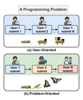
Figure 1: Comparison of User-Oriented and Problem-Oriented code optimization for the same problem.

⬇

#include <iostream>

#include <stdio.h>

using namespace std;

typedef long ll;

\parint main() {

int length;

ll arr[200000];

ll res[200000] = {0};

ll temp = 0;

ll m = 2147483647;

scanf("for (int i = 0; i < length; ++i) {

scanf("}

res[0] = arr[0];

for (int i = 1; i < length; ++i) {

res[i] += res[i - 1] + arr[i];

}

for (int i = 1; i < length; ++i) {

temp = abs(res[length - 1] - res[i - 1] * 2);

m = min(temp, m);

}

printf("return 0;

}

\par

(a) user1, initialization version.

⬇

#include <bits/stdc++.h>

using namespace std;

\par#define int long long

typedef vector<int> vi;

\parconst int INF = 1e18 + 5;

\parvoid solve() {

int n;

cin >> n;

vi v(n), pre(n);

int mn = INF, s = 0;

for(int i = 0; i < n; i++) cin >> v[i];

pre[0] = v[0];

for(int i = 1; i < n; i++) pre[i] = v[i] + pre[i - 1];

for(int i = n - 1; i >= 1; i–) {

s += v[i];

mn = min(mn, abs(pre[i - 1] - s));

}

cout << mn;

}

\parsigned main() {

speed;

int t = 1;

while(t–) solve();

}

(b) user1, iteration version.

⬇

#include<cstdio>

const int MAX = 2e5 + 5;

int a[MAX];

int main() {

int n;

long long sum = 0;

scanf("for (int i = 0; i < n; i++)

{

scanf("sum += a[i];

}

long long left,right,temp;

left = sum - a[n - 1];

right = a[n - 1];

long long min = left > right ? left - right : right - left;

left = 0;

for (int i = 0; i < n-2; i++) {

left += a[i];

right = sum - left;

temp = left > right ? left - right : right - left;

if (temp < min)

min=temp;

}

printf("return 0;

}

\par

(c) another user submitted version.

Figure 2: The three submitted code solutions all address problem "p03661", which asks for a split point in an array that minimizes the absolute difference between the sums of the two parts. Solutions (a) and (b) are different submissions from same user "u018679195". In (a), the prefix sum is calculated first, then the minimum difference is computed from start to finish. In (b), the prefix sum is also calculated first, but the minimum difference is computed from end to start, avoiding additional multiplication operations. Solution (c), from user "u353919145", calculates the difference between the left and right sums in real-time, requiring only one pass through the loop. It can be seen that solutions (a) and (b) only make local changes, while (c) constructs a more efficient algorithm.

1 Introduction

Code generation has become one of the most promising applications of LLMs and Code LLMs. Models such as GPT-4 Achiam et al. (2023), CodeLLama Roziere et al. (2023), StarCoder Li et al. (2023), WizardCoder Luo et al. (2024), and Deepseek-Coder Guo et al. (2024) have garnered great attention from academia and industry due to their remarkable code generation capabilities.

Despite their impressive code generation capabilities and high correct rate (Pass@k) in widely used benchmarks such as HumanEval Chen et al. (2021) and MBPP Austin et al. (2021), the code generated by these models is often not immediately usable in real-world scenarios. In practice, the code must also be optimized to meet specific constraints. For instance, in IoT applications where physical resources are limited, it is crucial to minimize code memory usage to ensure efficient operation Park and Kim (2024). Similarly, in low-latency scenarios such as high-frequency trading systems, the code must be optimized for time complexity and efficiency to handle large volumes of transactions swiftly and accurately Bilokon and Gunduz (2023). These practical scenarios highlight the need for code optimization to meet application requirements. Although low-level optimizing compilers and other performance engineering tools have made significant advancements Alfred et al. (2007); Wang and O’Boyle (2018), programmers still bear the primary responsibility for high-level performance considerations, including the selection of algorithms and APIs. However, automating high-level code optimization remains a significant challenge and has not been widely explored due to the need for understanding code semantics and performing optimizations accordingly.

Code optimization can proceed in many directions. In this paper, we focus on time performance optimization for practical considerations, aiming to minimize program execution time during the optimization process. Fortunately, Shypula et al. (2024) proposed the first program performance optimization dataset, PIE, which includes C++ programs designed to solve competitive programming problems, as C++ is a performance-oriented language. PIE tracks a single programmer’s submissions over time, identifying sequences of edits that lead to performance improvements. Each sample in the dataset consists of a pair of code solutions—a slow solution and a fast solution—submitted iteratively by the same user for the same problem. Meanwhile, Shypula et al. (2024) have preliminarily demonstrated the feasibility of adapting Code LLMs to code optimization through finetuning.

However, inspired by the iterative process of real software development and an in-depth observation and analysis of PIE, we found that this method of constructing code optimization pairs based on iterative submissions and optimizations by the same user for the same programming problem, although reflecting the direction of code optimization, is limited by the single programmer’s thought patterns. This often results in the program evolving and improving incrementally based on previous logic and paradigms. As shown in Figure 2, 2(a) and 2(b) are iterative submissions by the same user for the same problem. 2(b), compared to 2(a), did not change the overall algorithm but simply avoided some additional multiplication operations. In contrast, 2(c) is a submission by another user that presents a more efficient algorithm to solve the same problem.

In actual code review and refactoring processes, the original author of the code typically does not participate. Instead, these tasks are assigned to other programmers to avoid cognitive inertia, which can hinder significant improvements. In reality, it is often the clash of different perspectives that sparks innovation. When addressing the same programming problem, different programmers bring diverse viewpoints and approaches, leading to varied algorithms and paradigms. This insight inspired us to adopt a different approach. By shifting from an original author-oriented perspective to a problem-oriented perspective, we restructure the optimization pairs that were initially composed by the same programmer. The new problem-oriented optimization pairs integrate the diverse and innovative ideas of different programmers tackling the same problem. Experimental results show that adapting Code LLMs to problem-oriented optimization pairs significantly enhances their code optimization capabilities. However, while Code LLMs exhibit excellent optimization ratios and speedup under these pairs, further improvements are primarily constrained by correctness issues. To address this performance bottleneck, we draw inspiration from the idea that different models have their own strengths, and combining them can retain quality while providing additional benefits. Based on this idea, we utilize model merging to overcome this bottleneck, ultimately elevating the optimization ratio of from $51.76\%$ to $76.65\%$ and the speedup from $2.65\times$ to $5.09\times$, compared to the baseline.

To facilitate further exploration in code optimization, we have made the problem-oriented dataset, code, and evaluation scripts publicly available. In summary, our contributions are as follows:

• We thoroughly analyze the limitations of user-oriented program pairs and, for the first time, propose a problem-oriented perspective for code optimization.

• Adapting Code LLMs to problem-oriented program optimization pairs can significantly enhance the optimization ratio and Speedup across different Code LLMs and models with varying parameter scales.

• We identify the current performance bottlenecks in code optimization and achieve further breakthroughs through the method of model merging. Extensive experiments and analysis provide insights for the further development of the code optimization domain.

2 Related Works

2.1 LLMs for Code-Related Tasks.

LLMs pre-trained on extensive code corpora have exhibited impressive abilities in code generation and other code-related tasks Li et al. (2022); Nijkamp et al. (2023); Roziere et al. (2023); Wei et al. (2023); Guo et al. (2024). Numerous techniques and frameworks have been proposed to improve the accuracy of code generation, such as self-correction Chen et al. (2024); Zhong et al. (2024); Moon et al. (2024); Olausson et al. (2024). However, as mentioned earlier, the research of LLMs for code optimization, a domain that is both practically significant and highly challenging, has not yet been widely explored in both academia and industry.

2.2 Code Optimization.

Program optimization has been a major focus of software engineering for the past few decades Bacon et al. (1994); Kistler and Franz (2003). However, high-level optimizations such as algorithm changes remain elusive due to the difficulty of understanding the semantics of code. Previous machine learning has been applied to improve performance by identifying compiler transformations Bacon et al. (1994), optimizing GPU code Liou et al. (2020), and automatically selecting algorithms Kerschke et al. (2019). DeepPERF Garg et al. (2022) uses a transformer-based model fine-tuned to generate performance improvement patches for C# applications. Shypula et al. (2024) proposed the first new C++ dataset for program performance optimization. However, this dataset is user-oriented, which can lead to limitations due to localized optimization, overlooking the adoption of globally optimal algorithms and data structures.

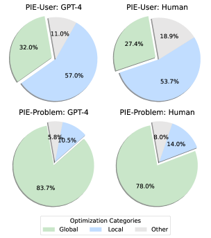
Figure 3: Statistical Analysis of Optimization Types.

3 Problem-Oriented Program Optimization Dataset

Shypula et al. (2024) constructed the PIE dataset, which focuses on optimizing program execution time based on human programmers’ submission for a range of competitive programming tasks from CodeNet Puri et al. (2021). The core idea behind the construction of PIE is that given a problem, programmers typically write an initial solution and iteratively improve it. Formally, $\mathbb{Y}^{u}_{x}=\left[y^{u}_{1},y^{u}_{2},...\right]$ be a chronologically sorted series of programs, written by user $u$ for the problem $x$. $\mathbb{Y}^{u}_{x}$ is removed for not accepted by the automated system, eliminating incorrect programs or take more than the allowed time to run, resulting in a trajectory of programs: $\mathbb{Y}^{u*}_{x}=[y^{u*}_{1},y^{u*}_{2},\ldots,y^{u*}_{n}]$. For each trajectory $\mathbb{Y}^{u*}_{x}$, construct pair $\mathbb{P}_{u}={(y^{u*}_{1},y^{u*}_{2}),(y^{u*}_{1},y^{u*}_{3}),(y^{u*}_{2},y^{u*}_{3})\ldots}$, and keep only pairs for which $\frac{\left(\texttt{time}\left({y_{i}}\right)-\texttt{time}\left({y_{>i}}\right)\right)}{\texttt{time}\left({y_{i}}\right)}>10\%$ where $\texttt{time}\left(y\right)$ is the measured latency of program $y$ (relative time improvements is more than 10%). Since all pairs in PIE are iterative versions submitted by the same user, we subsequently refer to this dataset as PIE-User. As shown in Figure 2, program optimization pairs in PIE-User, which consist of iterative submissions by the same user, can easily cause LLMs to focus on local performance improvements, neglecting global algorithmic advancements and innovations. Therefore, we restructured the PIE-User from a problem-oriented perspective. For each programming problem $x$, we collected valid submitted solutions by different users and sorted them based on benchmarked execution time (from slowest to fastest), resulting in another trajectory:

$$\mathbb{Y}^{p}_{x}=\left[y^{u_{1}}_{1},y^{u_{2}}_{1},y^{u_{3}}_{1},y^{u_{2}}_{2},y^{u_{3}}_{2},\ldots\right]$$

where $u_{1},u_{2},u_{3}$ represent different users, and $y^{u_{1}}_{1}$ represents the first valid submission by user $u_{1}$. It is evident that this trajectory interleaves submissions from different users. Based on the $\mathbb{Y}^{p}_{x}$, we reconstruct problem-oriented program performance optimization pairs as following:

$$\mathbb{P}_{p}= \{(y^{u_{1}}_{1},y^{u_{2}}_{1}),(y^{u_{1}}_{1},y^{u_{3}}_{1}),(y^{u_{1}}_{1},y^{u_{2}}_{2}),$$

$$(y^{u_{2}}_{1},y^{u_{2}}_{2}),(y^{u_{2}}_{1},y^{u_{3}}_{2}),\ldots\}$$

Dataset	Unique Problems	Pairs
PIE-User Train	1,135	56,086
PIE-Problem Train	336	14,051
Val	110	2,769
Test	80	1,422

Table 1: Number of unique problem ids and pairs.

t is important to note that we only retain program pairs in $\mathbb{P}_{p}$ that demonstrate a relative time improvement of greater than 90%. This is because, in code optimization engineering practice, an optimization that reduces the runtime by an order of magnitude compared to the pre-optimization runtime is generally considered global and significant Atwood (2012). We subsequently refer to this problem-oriented program optimization dataset as PIE-Problem. We retain the original validation and test sets without any changes to ensure fair comparisons in subsequent evaluations. The statistical results of the PIE-Problem are shown in the Table 1. We meticulously reviewed and ensured that any particular competitive programming problem appeared in only one of the train, validation, or test sets. It can be seen that the PIE-Problem program optimization pairs are fewer than the original PIE-User pairs. This is because problem-oriented program pairs have a high threshold, with each achieving at least a 90% relative time improvement.

Furthermore, we randomly selected 1,000 program optimization pairs from the PIE-User and PIE-Problem datasets for analysis by GPT-4, and 100 pairs for human analysis to identify the types of optimizations made. The results are categorized into three types: global algorithmic optimizations, local optimizations, and others (such as code cleanup), as shown in Figure 3 (details are provided in Appendix A). For PIE-User, true global algorithmic optimizations account for a relatively small proportion. In contrast, most of the program pairs in PIE-Problem fall into the "global algorithm optimization" category. Moreover, GPT-4 identifies a higher proportion of "global algorithm optimization" compared to human analysis. Upon observation and comparison, we find that this discrepancy is mainly because GPT-4 tends to classify program pairs with large changes as "global algorithm optimization".

Table 2: Main Results: Prompt and Fine-Tuning for various LLMs with best@1 and best@8.

Prompt		Best@1			Best@8
/ Dataset	Model	%Opt	Speedup	Correct	%Opt	Speedup	Correct
Instruct	CodeLlama 34B	0.70%	1.002$\times$	24.50%	5.70%	1.048$\times$	88.96%
Instruct	DeepSeek-Coder 33B	2.88%	1.016$\times$	16.17%	11.53%	1.091$\times$	68.00%
Instruct	GPT-3.5	7.10%	1.049$\times$	68.35%	11.60%	1.073$\times$	81.65%
Instruct	GPT-4	8.37%	1.062$\times$	65.33%	16.81%	1.149$\times$	93.74%
CoT	CodeLlama 34B	1.27%	1.017$\times$	16.17%	9.85%	1.103$\times$	79.75%
CoT	DeepSeek-Coder 33B	4.64%	1.042$\times$	14.91%	16.81%	1.178$\times$	61.89%
CoT	GPT-4	13.43%	1.173$\times$	48.65%	27.92%	1.246$\times$	84.53%
PIE-User	CodeLlama 7B	12.80%	1.452$\times$	30.45%	35.65%	2.051$\times$	78.27%
PIE-User	CodeLlama 13B	16.03%	1.402$\times$	31.79%	34.46%	1.998$\times$	77.36%
PIE-User	CodeLLama 34B	14.14%	1.435$\times$	36.57%	37.06%	2.089$\times$	81.79%
PIE-User	DeepSeek-Coder 7B	23.56%	1.596$\times$	51.27%	44.23%	2.327$\times$	86.23%
PIE-User	DeepSeek-Coder 33B	27.57%	1.770$\times$	59.49%	51.76%	2.649$\times$	91.14%
PIE-Problem	CodeLlama 7B	9.85%	1.468$\times$	10.27%	33.12%	2.616$\times$	34.23%
PIE-Problem	CodeLlama 13B	10.06%	1.485$\times$	10.62%	36.71%	2.886$\times$	38.05%
PIE-Problem	CodeLLama 34B	13.08%	1.686$\times$	13.57%	44.02%	3.401$\times$	45.29%
PIE-Problem	DeepSeek-Coder 7B	30.38%	2.558$\times$	31.08%	68.50%	4.679$\times$	70.18%
PIE-Problem	DeepSeek-Coder 33B	36.64%	2.963$\times$	37.41%	71.03%	4.812$\times$	72.50%

4 Experiment Setting

Code LLMs Selection.

We select CodeLLama (7B, 13B, 34B) Roziere et al. (2023) and DeepSeek-Coder (7B, 33B) Guo et al. (2024) for code optimization. CodeLLama is the most widely used Code LLM, while DeepSeek-Coder is currently the best-performing Code LLM. We use LoRA Hu et al. (2022), a parameter-efficient fine-tuning method, to adapt Code LLMs for code optimization. Detailed training parameters are provided in the Appendix B.

Test Cases and Execution Time Measurement.

We evaluate the correctness of the optimized programs through unit tests; any program that fails a single test is rejected. For PIE-Problem, we use the same test cases as PIE-User, averaging 88.1 per problem in the training set, 75 per problem in the validation set, and 104 per problem in the test set. Accurately evaluating the execution time of a program is a critical issue, as measurements of time on real hardware can significantly vary due to server workload and configuration problems. We measure the execution time of each program utilizing gem5 CPU simulators Binkert et al. (2011), which serves as the gold standard for CPU simulation in both academia and industry, ensuring entirely deterministic and reliable results and reproducibility.

Metrics.

To evaluate performance, we measure below metrics for functionally correct programs:

• Percent Optimized $\mathbf{[\textsc{\%Opt}]}$: The fraction of programs in the test set (out of 1422 unseen samples) improved by a certain method. A program must be at least 10% faster and correct to contribute.

• Speedup $\mathbf{[\textsc{Speedup}]}$: The absolute improvement in running time. If $o$ and $n$ are the “old” and “new” running times, then $\textsc{speedup(o, n)}=\left(\frac{o}{n}\right)$. A program must be correct to contribute.

• Percent Correct [Correct]: The proportion of programs in the test set that are at least functionally equivalent to the original program (included as an auxiliary analysis metric).

We count a program as functionally correct if it passes every test case. Notably, %Opt and Speedup are the main metrics, and they are calculated for the entire test set. While Correct is not our primary focus, we include it to aid interpreting our results. Additionally, we report our Speedup as the average speedup across all test set samples. For generated programs that are either incorrect or slower than the original, we use a speedup of 1.0 for that example, as the original program, in the worst case, has a speedup of 1.0. We benchmark performance using gem5 environment and all test cases. We compile all C++ programs with GCC version 9.4.0 and C++17 as well as the -O3 optimization flag; therefore, any reported improvements would be those on top of the optimizing compiler.

Figure 4: Instruct Prompt.

Decoding strategy.

Code generation benefits from sampling multiple candidate outputs for each input and selecting the best one; in our case, the "best" is the fastest program that passes all test cases. We use best@$k$ to denote this strategy with $k$ samples and a temperature of 0.7.

5 Main Results and Discussion

Table 2 presents the main results of using prompts and adapting Code LLMs for code optimization based on PIE-User and PIE-Problem, respectively.

Instruct and CoT prompting.

First, we adopt the most straightforward way by directly using an instruct prompt to have the LLMs generate optimized code. The instruct prompt is shown in Figure 4. Additionally, inspired by Chain-of-Thought (CoT) prompting Wei et al. (2022), we ask the LLMs to think about how to optimize the program before actually generating the optimized program (details of the CoT prompt are shown in the Appendix D). The result shows that using instruct prompt and CoT did not significantly improve %Opt and Speedup for code optimization. The best performance by GPT-4 (CoT) achieved 27.92 %Opt and 1.246$\times$ Speedup. Additionally, we observe that when LLMs perform optimization under CoT, generating an optimized program based on the strategy can lead to a certain degree of decline in correctness. This suggests that while CoT helps in Speedup, it may introduce complexities that affect the overall correctness of generated code.

Adapting Code LLMs on PIE-User and PIE-Problem.

When fine-tuning Code LLMs using PIE-User, we adopt the best performance-conditioned generation method proposed by (Shypula et al., 2024). This method involves informing the model in the instructions about the extent to which the current optimized code has achieved the best performance(details and our considerations are in Appendix C). In contrast, when fine-tuning using PIE-Problem, we opt for the simplest instruction, as shown in Figure 4, as we believe that "the simpler the better" in practice. From Table 2, it can be seen that for the two key metrics %Opt and Speedup, Code LLMs perform significantly better on PIE-Problem compared to PIE-User, with the only exception being the CodeLlama series, which shows a slight decline in %Opt under best@1. This is primarily due to the performance bottleneck issue (explained below). Among them, the best-performing Code LLM, DeepSeek-Coder 33B, increased %Opt from 51.76% to 71.03% and Speedup from 2.649$\times$ to 4.812$\times$ under best@8.

Table 3: Problem-Oriented experiments for various Code LLMs with best@1 and best@8.

		Best@1			Best@8
Model	Method	%Opt	Speedup	Correct	%Opt	Speedup	Correct
CodeLLama 34B	PIE-Problem	13.08%	1.686$\times$	13.57%	44.02%	3.401$\times$	45.29%
CodeLlama 34B	Self-Correct	13.85%	1.703$\times$	14.21%	45.35%	3.463$\times$	47.47%
CodeLlama 34B	Curriculum-Learning	12.45%	1.551$\times$	13.15%	43.74%	3.285$\times$	45.43%
CodeLlama 34B	Merge-Slerp	17.65%	1.805$\times$	19.13%	51.05%	3.613$\times$	54.85%
CodeLlama 34B	Merge-Linear	18.14%	1.832$\times$	21.21%	56.53%	3.830$\times$	64.28%
DeepSeek-Coder 7B	PIE-Problem	30.38%	2.558$\times$	31.08%	68.50%	4.679$\times$	70.18%
DeepSeek-Coder 7B	Self-Correct	32.13%	2.601$\times$	32.98%	68.97%	4.712$\times$	70.67%
DeepSeek-Coder 7B	Curriculum-Learning	27.11%	2.325$\times$	28.69%	63.43%	4.506$\times$	65.68%
DeepSeek-Coder 7B	Merge-Slerp	35.30%	2.477$\times$	44.80%	70.04%	4.638$\times$	74.68%
DeepSeek-Coder 7B	Merge-Linear	38.40%	2.770$\times$	43.53%	70.46%	4.732$\times$	75.53%
DeepSeek-Coder 33B	PIE-Problem	36.64%	2.963$\times$	37.41%	71.03%	4.812$\times$	72.50%
DeepSeek-Coder 33B	Self-Correct	37.76%	3.031$\times$	39.45%	73.12%	4.902$\times$	74.19%
DeepSeek-Coder 33B	Curriculum-Learning	31.15%	2.579$\times$	32.28%	68.14%	4.692$\times$	70.18%
DeepSeek-Coder 33B	Merge-Slerp	43.60%	3.095$\times$	45.71%	75.32%	5.037$\times$	77.22%
DeepSeek-Coder 33B	Merge-Linear	46.69%	3.432$\times$	48.03%	76.65%	5.087$\times$	78.76%

Insight of optimization pairs.

Tale 2 shows that transitioning program optimization pairs from User-Oriented to Problem-Oriented brings significant improvements in code optimization by Code LLMs. Despite being relatively small, PIE-Problem enables LLMs to learn better program optimization capabilities. This indicates that for program optimization, high-quality global program optimization pairs are more important than quantity.

Insight on different Code LLMs and parameter scales.

We observe significant differences in code optimization performance across various Code LLM series. The best CodeLlama model (CodeLlama 34B) lags behind the top-performing DeepSeek-Coder model (DeepSeek-Coder 33B) by 27.01% in %Opt and 1.411$\times$ in Speedup. Additionally, it is surprising that the DeepSeek-Coder 7B significantly outperforms CodeLlama 34B. We believe this disparity is mainly due to the high level of code semantic understanding required for code optimization tasks. Only when a Code LLM’s understanding of code reaches a certain level can it perform efficient optimization. Therefore, any differences in code comprehension among Code LLMs will further amplify their differences in code optimization capabilities. The relationship between code understanding and code optimization warrants further exploration.

Insight of correctness and performance bottleneck.

From the Correct column in Table 2, it can be seen that under PIE-Problem fine-tuning, Code LLMs experiences a noticeable decline in correctness compared to under PIE-User fine-tuning and prompt methods. Although correctness is not the main metric, it provides additional insights. It can be seen that under PIE-Problem fine-tuning, Code LLMs show very close performance metrics for %Opt and correctness, a phenomenon not observed under PIE-User fine-tuning and prompt methods. This indicates that with PIE-Problem fine-tuning, Code LLMs almost always achieve a speedup effect (95%+) as long as the generated optimized program is functionally correct. However, under PIE-User fine-tuning or prompt methods, this is not the case (%Opt and correctness show a large gap), resulting in many programs that are functionally correct but do not exhibit a significant speedup effect. Therefore, the performance bottleneck for code optimization in Code LLMs under PIE-Problem fine-tuning lies in correctness. To improve %Opt and Speedup, the focus should be on enhancing correctness.

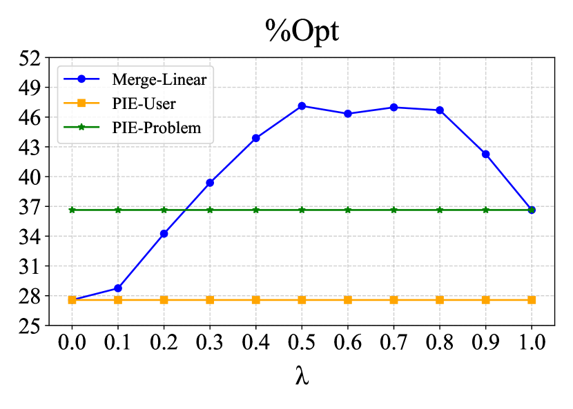
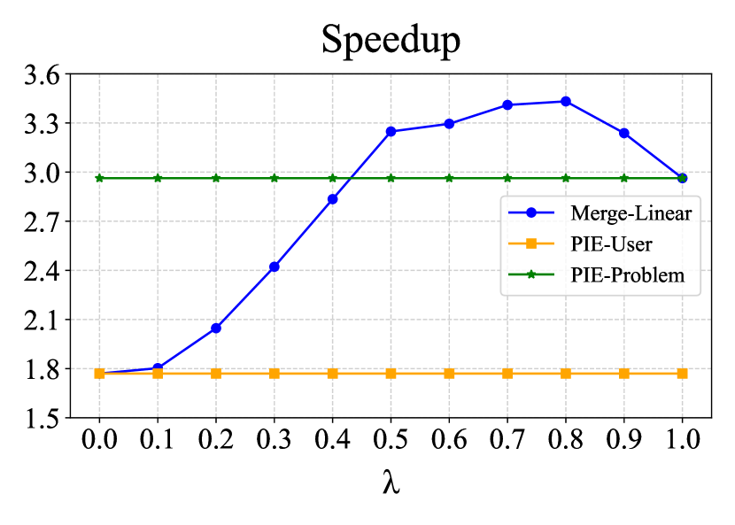
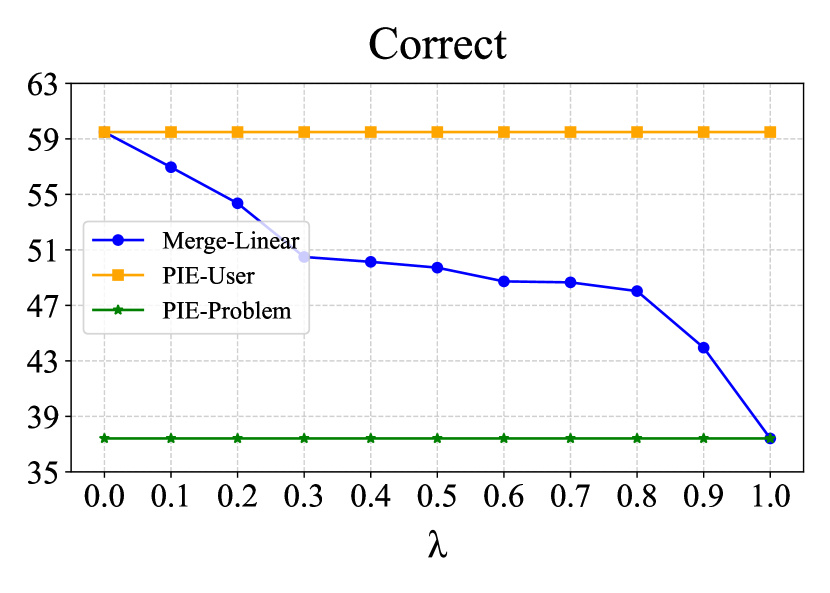
Figure 5: Analysis of Merge Weights for Deepseek-Coder 33B on best@1.

6 Overcoming Performance Bottlenecks

Considering that the correctness of Code LLMs remains at a high level under PIE-User fine-tuning, we believe this optimization direction is overly conservative. On the other hand, the performance bottleneck of Code LLMs under PIE-Problem fine-tuning lies in correctness, indicating an overly aggressive optimization direction. This suggests that the optimization directions of the two methods are different. This inspired us to combine the strengths of both by merging the two Code LLMs into a single Code LLM, thereby retaining the original capabilities while gaining additional benefits. We choose two main LLM merging methods for our experiment: Merge-Linear Wortsman et al. (2022) and Merge-Slerp. Additionally, we compared the model merge methods with two other intuitive approaches. The first is Self-Correct. In code generation, Self-Correct is an important method for improving correctness. This involves having Code LLMs review and debug their own generated programs to achieve self-correction Chen et al. (2024); Zhong et al. (2024). Furthermore, for the challenging task of code optimization, we apply curriculum learning Pattnaik et al. (2024). This approach involves the model first learning from easier samples and then progressing to more complex ones. Specifically, we fine-tune the Code LLMs on the easier PIE-User dataset first, and then move on to the harder PIE-Problem dataset.

Results on Code LLMs merge and baselines.

Table 3 presents the experimental results of model merging, Self-Correct, and curriculum learning. Firstly, the Self-Correct method provides limited improvement in correctness, which only relatively enhances %Opt and Speedup. Through manual analysis, we find that Code LLMs tend to focus on local areas of the code during self-debugging, leading to an insufficient understanding of the code’s overall semantics and, consequently, ineffective corrections. On the other hand, curriculum learning negatively impacts code optimization. We speculate that this is mainly because, in code optimization, the optimization spaces for simple user-oriented tasks and complex problem-oriented tasks can be entirely different. The optimization methods learned in the user-oriented perspective may not effectively apply to the problem-oriented perspective when continue finetuning. This may even limit the model’s flexibility and innovative capability when facing complex tasks due to fixed thinking patterns, leading to performance degradation. In contrast, model merge can avoid the drawbacks of fixed thinking patterns by fully leveraging the advantages of each model, resulting in the merged LLM with stronger overall capabilities. Particularly, Merge-Linear significantly improves correctness, thereby enhancing %Opt and Speedup. In Deepseek-Coder 33b (Merge-Linear), %Opt further increases from 36.64% to 46.69%, and Speedup improves from 2.96$\times$ to $3.43\times$ on best@1 compared to Deepseek-Coder 33B fine-tuned solely on PIE-Problem.

7 Detailed Analysis

7.1 Merge Weight Analysis

In model merging, there is a weight parameter $\lambda$, used to adjust the proportion of two LLMs’ parameters. To comprehensively analyze the impact of this weight on the final code optimization performance, we conduct a detailed study using Deepseek-Coder 33B. The parameter $\lambda$ represents the weight of Deepseek-Coder 33B fine-tuned on PIE-Problem, while $(1-\lambda)$ represents the weight of Deepseek-Coder 33B fine-tuned on PIE-User. The experimental results are shown in Figure 5. We find that within the range of $\lambda$ values from 0.5 to 0.8, the merged model shows significant improvements in %Opt and Speedup compared to fine-tuning solely on PIE-Problem. In this range, correctness remains relatively stable without significant fluctuations. However, when the $\lambda$ value is too large (> 0.8), correctness decreases significantly, leading to performance bottlenecks. Similarly, when the $\lambda$ value is too small (< 0.5), the model weights under PIE-User fine-tuned dominate, which also negatively impacts %Opt and Speedup.

Table 4: Error analysis.

Result	Percentage
Failed to compile	24.70%
Compiled, but test cases wrong	66.27%
Correct, but slower	3.01%
Correct, but not $>$1.1$\times$ Speedup	6.02%

7.2 Error Analysis

We performed an error analysis on the Deepseek-Coder 33B with Merge-Linear version, examining the generated programs that failed to optimize and identifying the cause of each failure. Table 4 shows that $\sim$25% of the programs failed to compile, and a significant portion ($\sim$66%) failed because the optimized program broke a test case. Additionally, about 3% of the programs are slower, and 6% did not meet the speedup threshold of 10%. These findings suggest a potential future direction where techniques from more powerful program repair could be combined with PIE-Problem for better optimization performance.

8 Conclusion

In this paper, we propose shifting the perspective of code optimization from User-Oriented to Problem-Oriented and introduce the PIE-Problem dataset. This new perspective brings significant improvements in the optimization ratio and speedup. Additionally, we identified current performance bottlenecks in code optimization and achieved further breakthroughs through model merging. Our approach and insights pave an exciting and feasible path for enhancing program efficiency.

9 Limitation

This paper focuses on optimizing the time efficiency of given code, without considering other optimization directions. However, in real-world scenarios, there are many other optimization directions, such as memory optimization. Additionally, the code optimization in this paper is based on a given code, whereas directly generating the most time-efficient program from a natural language problem is a more natural and challenging issue that warrants further research.

Appendix A Categories of Optimization Types.

We categorize code optimization into three main categories: global algorithmic optimizations, local optimizations, and other optimizations.

• Global Algorithmic Optimizations: This type of optimization involves altering the algorithm itself to achieve significant performance improvements. Such changes can effectively reduce time complexity and enhance the speed of code execution. Examples include transforming recursive solutions into dynamic programming approaches, leveraging advanced mathematical theories, and restructuring complex data processing logic. These optimizations can lead to substantial gains in efficiency and scalability.

• Local Optimizations: These optimizations focus on improving specific parts of the code without changing the overall algorithm. They include enhancing I/O functions, optimizing read/write patterns to minimize runtime delays, and reducing computational complexity in certain sections of the code. By addressing these localized issues, programs can achieve more efficient execution and better resource utilization, ultimately leading to faster and more responsive applications.

• Other Optimizations: This category involves general code cleanup and refactoring aimed at improving code readability, maintainability, and overall quality. Examples include removing unnecessary initializations and redundant code, cleaning up outdated comments, and organizing the code structure more logically.

We randomly selected 1,000 pairs of program optimizations from the PIE-User and PIE-Problem datasets for analysis by GPT-4, and 100 pairs for analysis by humans. The classification process followed the three types mentioned above, and the results are shown in Figure 3.

Appendix B Training Details.

We fine-tuned the CodeLlama series (7B, 13B, 34B) and the Deepseek-Coder series (7B, 33B) on a server with 4$\times$A100 GPUs (NVIDIA A100 80GB). During the fine-tuning process, we used LoRA Hu et al. (2022) (lora_rank=8, lora_target=$\left[q\_proj,v\_proj\right]$), and for both PIE-User and PIE-Problem dataset, we only trained for 2 epochs. All experiments were conducted using AdamW Loshchilov and Hutter (2019) optimizer with an initial learning rate of 5e-5.

Appendix C Performance-conditioned Generation.

Shypula et al. (2024) introduced performance tags during training by associating each "fast" program with a tag indicating the optimal achievable performance across all solutions in the PIE-User dataset, as shown in Figure 6. This approach has demonstrated the best fine-tuning results. Therefore, we adopted this method for fine-tuning Code LLMs on the PIE-User dataset, and the experimental results for PIE-User are reported using performance-conditioned generation by default. However, we believe that this performance tag approach relies on the ranking of the current solution among existing solutions. For a given problem, the current solutions may not necessarily be optimal, and thus, introducing performance tags could lead to incorrect associations. Therefore, when fine-tuning the PIE-Problem dataset, we used the simplest and most straightforward instruction, as shown in Figure 4.

Figure 6: Training (top) and inference (bottom) prompts for performance-conditioned generation.

Appendix D CoT Prompting.

Inspired by Chain-of-Thought (CoT) prompting Wei et al. (2022), we first have the LLMs propose improvement strategies based on the slow program, and then generate the optimized program using both the slow program and the proposed strategies. The specific CoT prompt is shown in Figure 7.

Figure 7: Chain-of-thought prompting.

Appendix E More Inspiring Examples.

We provide additional examples, as shown in Figure 8, Figure 9, and Figure 10, to illustrate that in the original PIE-User, program optimization pairs are constructed through iterative submissions and optimizations by the same user for the same programming problem, which can be limited by the single programmer’s thought patterns.

⬇

#include <bits/stdc++.h>

\parusing namespace std;

\par#define int long long

\parconst int N = 1e5 + 5, M = 5, inf = 1e15;

\parint dp[N][M], a[N];

\parchar op[N];

\parint Sign(int x) {

if (x return 1;

}

\parint32_t main() {

for (int i = 0; i < N; i++) for (int j = 0; j < M; j++) dp[i][j] = -inf;

int n; cin >> n >> a[0];

for (int i = 1; i < n; i++) cin >> op[i] >> a[i];

dp[0][0] = a[0];

for (int i = 1; i < n; i++) for (int j = M - 1; j >= 0; j–) {

if (op[i] == ’+’) dp[i][j] = dp[i - 1][j] + a[i] * Sign(j);

else if (j) dp[i][j] = dp[i - 1][j - 1] + a[i] * Sign(j);

if (j + 1 < M) dp[i][j] = max(dp[i][j], dp[i][j + 1]);

}

cout << dp[n-1][0] << "\n";

}

\par

(a) user1, initialization version.

⬇

#include <bits/stdc++.h>

using namespace std;

\par#define int long long

const int N = 1e5 + 5, M = 3, inf = 1e15;

\parint dp[N][M], a[N];

char op[N];

\parint Sign(int x) {

if (x return 1;

}

\parint32_t main() {

ios::sync_with_stdio(0), cin.tie(0), cout.tie(0), cout.tie(0);

for (int i = 0; i < N; i++) for (int j = 0; j < M; j++) dp[i][j] = -inf;

int n; cin >> n >> a[0];

for (int i = 1; i < n; i++) cin >> op[i] >> a[i];

dp[0][0] = a[0];

for (int i = 1; i < n; i++) for (int j = M - 1; j >= 0; j–) {

if (op[i] == ’+’) dp[i][j] = dp[i - 1][j] + a[i] * Sign(j);

else if (j) dp[i][j] = dp[i - 1][j - 1] + a[i] * Sign(j);

if (j + 1 < M) dp[i][j] = max(dp[i][j], dp[i][j + 1]);

}

cout << dp[n-1][0] << "\n";

}

\par\par

(b) user1, iteration version.

⬇

#include<cstdio>

#include<algorithm>

using namespace std;

const int MAXN=int(1e5+5);

typedef long long LL;

#define INF LL(1e15)

LL s1,s2,as,n;

LL sz[MAXN],fh[MAXN];

char c[5];

int main()

{

scanf("scanf("getchar();

for(LL i=1;i<=n-1;i++) {

scanf("scanf("fh[i]=c[0];

}

s1=s2=-INF;

for(LL i=1;i<=n-1;i++) {

if(fh[i]==’-’) {

as-=sz[i];

s1-=sz[i];

s2+=sz[i];

s1=max(s1,s2);

s2=max(as,s2);

}

else {

as+=sz[i];

s1+=sz[i];

s2-=sz[i];

}

s2=max(s1,s2);

as=max(s2,as);

}

printf("}

\par\par\par\par

(c) another user submitted version.

Figure 8: The above three code snippets all come from the problem "p03580", which involves maximizing the evaluated value of a given formula by adding an arbitrary number of pairs of parentheses and outputting the maximum possible value. (a) and (b) are from the same user "u1821171064", both employing dynamic programming algorithms with a time complexity of $\mathcal{O}\left(N*M\right)$, where N is the length of the sequence and M is the number of states. In (b), the number of states M is reduced, and input and output are optimized. (c) is from user "u863370423" and uses a greedy algorithm, which is suitable for problems with fewer current states where the global optimal solution can be achieved through local optimization, with a time complexity of $\mathcal{O}\left(N\right)$.

⬇

#include <iostream>

#include <cstring>

using namespace std;

typedef long long LL;

#define F(i) for(int i=0;i<n;i++)

\parint d[555][555] = {0}, c[555][555] = {0};

\parint qu(int l, int r) {

if (l > r) return 0;

if (d[l][r] != -1) return d[l][r];

return d[l][r] = c[l][r] + qu(l + 1, r) + qu(l, r - 1) - qu(l + 1, r - 1);

}

\parint main() {

memset(d, -1, sizeof(d));

int n, m, q;

cin >> n >> m >> q;

while (m–) {

int l, r;

cin >> l >> r;

c[l][r]++;

}

while (q–) {

int l, r;

cin >> l >> r;

cout << qu(l, r) << endl;

}

return 0;

}

\par

(a) user1, initialization version.

⬇

#include <bits/stdc++.h>

using namespace std;

\par#define int long long

#define pb push_back

#define faster ios::sync_with_stdio(0)

\parconst int N = 509;

vector<int> v[N + 5];

\parint32_t main() {

faster;

int n, p, q;

cin >> n >> p >> q;

int x, y;

for (int i = 1; i <= p; i++) {

cin >> x >> y;

v[x].pb(y);

}

for (int i = 1; i <= n; i++) {

sort(v[i].begin(), v[i].end());

}

while (q–) {

cin >> x >> y;

int ans = 0;

for (int i = x; i <= y; i++) {

ans += upper_bound(

v[i].begin(), v[i].end(), y)

- v[i].begin();

}

cout << ans << "\n";

}

return 0;

}

\par

(b) user1, iteration version.

⬇

#include <cstdio>

#define int long long

#define dotimes(i, n) for (int i = 0; i < (n); i++)

\parusing namespace std;

\parint rint() {

int n;

scanf("return n;

}

\parvoid wint(int n) {

printf("}

\parsigned main() {

int N = rint();

int M = rint();

int Q = rint();

int S[N + 1][N + 1];

dotimes(R, N + 1)

dotimes(L, N + 1)

S[R][L] = 0;

dotimes(i, M) {

int L = rint();

int R = rint();

S[R][L]++;

}

dotimes(R, N)

dotimes(L, N)

S[R + 1][L + 1] += S[R + 1][L] + S[R][L + 1] - S[R][L];

dotimes(i, Q) {

int p = rint() - 1;

int q = rint();

wint(S[q][q] + S[p][p] - S[q][p] - S[p][q]);

}

return 0;

}

\par\par

(c) another user submitted version.

Figure 9: The above three code segments all come from the same problem "p03283", which deals with cumulative sum queries in a 2D matrix. (a) and (b) are different submission versions from the same user "u816631826". In (a), the problem is solved using recursion and dynamic programming, but the query time complexity is high, $\mathcal{O}\left(N^{2}\right)$. In (b), the STL-provided binary search function is used, reducing the time complexity to $\mathcal{O}\left(N*\log(N)\right)$. (c) comes from another user "u281670674" and solves the problem using a 2D prefix sum matrix. The preprocessing time complexity is $\mathcal{O}\left(N^{2}\right)$, but the query time complexity for each query is $\mathcal{O}\left(1\right)$, making it more efficient.

⬇

#include <bits/stdc++.h>

\parusing namespace std;

\parinline void rd(int &x) {

char ch;

for(;!isdigit(ch=getchar()););

for(x=ch-’0’;

isdigit(ch=getchar());)

x=x*10+ch-’0’;

}

\partypedef long long LL;

\parconst int MAXN = 300005;

\parint N, n, a[MAXN], cnt[MAXN];

\parLL sum[MAXN];

\parint ans[MAXN];

\parinline bool chk(int k, int x) {

int pos = upper_bound(a + 1, a + n + 1, x) - a;

return sum[pos-1] + 1ll*(n-pos+1)*x >= 1ll*k*x;

}

\parint main() {

rd(N);

for(int i = 1, x; i <= N; ++i) rd(x), ++cnt[x];

for(int i = 1; i <= 300000; ++i) if(cnt[i]) a[++n] = cnt[i];

sort(a + 1, a + n + 1);

for(int i = 1; i <= n; ++i) sum[i] = sum[i-1] + a[i];

int now = 0;

for(int k = n; k >= 1; –k) {

while(now < N && chk(k, now+1)) ++now;

ans[k] = now;

}

for(int i = 1; i <= N; ++i) printf("}

\par\par

(a) user1, initialization version.

⬇

#include <bits/stdc++.h>

\parusing namespace std;

\parinline void rd(int &x) {

char ch;

for(;!isdigit(ch=getchar()););

for(x=ch-’0’;

isdigit(ch=getchar());)

x=x*10+ch-’0’;

}

\partypedef long long LL;

\parconst int MAXN = 300005;

\parint n, cnt[MAXN];

\parLL sum[MAXN];

\parint ans[MAXN];

\parinline bool chk(int k, int x) { return sum[x] >= 1ll*k*x; }

\parint main() {

rd(n);

for(int i = 1, x; i <= n; ++i) rd(x), ++cnt[x], ++sum[cnt[x]];

for(int i = 1; i <= n; ++i) sum[i] += sum[i-1];

int now = 0;

for(int k = n; k >= 1; –k) {

while(now < n && chk(k, now+1)) ++now;

ans[k] = now;

}

for(int i = 1; i <= n; ++i) printf("}

\par\par\par

(b) user1, iteration version.

⬇

#include<bits/stdc++.h>

#include<cstdio>

using namespace std;

typedef long long ll;

#define rep(i, n) for(int i = 0; i < (n); i++)

#define rep1(i, n) for(int i = 1; i <= (n); i++)

\parint hist[300002], cnt[300001];

const int cm = 1 << 17;

char cn[cm], * ci = cn + cm, ct;

\parinline char getcha() {

if (ci - cn == cm) { fread_unlocked(cn, 1, cm, stdin); ci = cn; }

return *ci++;}

inline int getint() {

int A = 0;

if (ci - cn + 16 > cm) while ((ct = getcha()) >= ’0’) A = A * 10 + ct - ’0’;

else while ((ct = *ci++) >= ’0’) A = A * 10 + ct - ’0’;

return A;}

\parconst int dm = 1 << 21;

char dn[dm], * di = dn;

inline void putint(int X) {

int keta = 0;

char C[10];

while (X) {

*(C + keta) = ’0’ + X X /= 10;

keta++;

}

for (int i = keta - 1; i >= 0; i–)* di++ = (*(C + i));

*di++ = ’\n’;}

\parint main() {

int N = getint();

rep(i, N) hist[getint()]++;

rep1(i, N) cnt[hist[i]]++;

int k = 1;

rep(i, N + 1) rep(j, cnt[i]) hist[k++] = i

\park = N + 1;

int ruiseki = N;

int mae = 0;

for (int i = N; i >= 1; i–) {

while (hist[k - 1] >= i) {

ruiseki -= hist[–k];

}

int kei = N - k + 1 + ruiseki / i;

\parfor (int j = mae + 1; j <= kei; j++) putint(i);

mae = kei;

}

for (int j = mae + 1; j <= N; j++) {

*di++ = ’0’;

*di++ = ’\n’;

}

fwrite(dn, 1, di - dn, stdout);

return 0;

}

\par\par\par

(c) another user submitted version.

Figure 10: The above three code snippets all come from the problem "p02890", which requires calculating, for each possible K value (from 1 to N), the maximum number of times K cards with different numbers can be selected and removed from N cards. (a) and (b) are from the same user "u990400947" and utilize prefix sum calculation and searching. The latter employs condition checking with a time complexity of $\mathcal{O}\left(N*\log(N)\right)$. (c) uses a difference array, reducing the time complexity to $\mathcal{O}\left(N\right)$.

References

- Achiam et al. (2023) Josh Achiam, Steven Adler, Sandhini Agarwal, Lama Ahmad, Ilge Akkaya, Florencia Leoni Aleman, Diogo Almeida, Janko Altenschmidt, Sam Altman, Shyamal Anadkat, et al. 2023. Gpt-4 technical report. arXiv preprint arXiv:2303.08774.
- Alfred et al. (2007) V Aho Alfred, S Lam Monica, and D Ullman Jeffrey. 2007. Compilers Principles, Techniques & Tools. pearson Education.
- Atwood (2012) Jeff Atwood. 2012. Effective Programming: More Than Writing Code: Your one-stop shop for all things programming. Hyperink Inc.
- Austin et al. (2021) Jacob Austin, Augustus Odena, Maxwell Nye, Maarten Bosma, Henryk Michalewski, David Dohan, Ellen Jiang, Carrie Cai, Michael Terry, Quoc Le, et al. 2021. Program synthesis with large language models. arXiv preprint arXiv:2108.07732.
- Bacon et al. (1994) David F. Bacon, Susan L. Graham, and Oliver J. Sharp. 1994. Compiler transformations for high-performance computing. ACM Comput. Surv., 26(4):345–420.
- Bilokon and Gunduz (2023) Paul Bilokon and Burak Gunduz. 2023. C++ design patterns for low-latency applications including high-frequency trading.
- Binkert et al. (2011) Nathan Binkert, Bradford Beckmann, Gabriel Black, Steven K Reinhardt, Ali Saidi, Arkaprava Basu, Joel Hestness, Derek R Hower, Tushar Krishna, Somayeh Sardashti, et al. 2011. The gem5 simulator. ACM SIGARCH computer architecture news, 39(2):1–7.
- Chen et al. (2021) Mark Chen, Jerry Tworek, Heewoo Jun, Qiming Yuan, Henrique Ponde de Oliveira Pinto, Jared Kaplan, Harri Edwards, Yuri Burda, Nicholas Joseph, Greg Brockman, et al. 2021. Evaluating large language models trained on code. arXiv preprint arXiv:2107.03374.
- Chen et al. (2024) Xinyun Chen, Maxwell Lin, Nathanael Schärli, and Denny Zhou. 2024. Teaching large language models to self-debug. In The Twelfth International Conference on Learning Representations.
- Garg et al. (2022) Spandan Garg, Roshanak Zilouchian Moghaddam, Colin B. Clement, Neel Sundaresan, and Chen Wu. 2022. Deepperf: A deep learning-based approach for improving software performance.
- Guo et al. (2024) Daya Guo, Qihao Zhu, Dejian Yang, Zhenda Xie, Kai Dong, Wentao Zhang, Guanting Chen, Xiao Bi, Y Wu, YK Li, et al. 2024. Deepseek-coder: When the large language model meets programming–the rise of code intelligence. arXiv preprint arXiv:2401.14196.
- Hu et al. (2022) Edward J Hu, yelong shen, Phillip Wallis, Zeyuan Allen-Zhu, Yuanzhi Li, Shean Wang, Lu Wang, and Weizhu Chen. 2022. LoRA: Low-rank adaptation of large language models. In International Conference on Learning Representations.
- Kerschke et al. (2019) Pascal Kerschke, Holger H. Hoos, Frank Neumann, and Heike Trautmann. 2019. Automated algorithm selection: Survey and perspectives. Evolutionary Computation, 27(1):3–45.
- Kistler and Franz (2003) Thomas Kistler and Michael Franz. 2003. Continuous program optimization: A case study. ACM Trans. Program. Lang. Syst., 25(4):500–548.
- Li et al. (2023) Raymond Li, Loubna Ben allal, Yangtian Zi, Niklas Muennighoff, Denis Kocetkov, Chenghao Mou, Marc Marone, Christopher Akiki, Jia LI, Jenny Chim, Qian Liu, Evgenii Zheltonozhskii, Terry Yue Zhuo, Thomas Wang, Olivier Dehaene, Joel Lamy-Poirier, Joao Monteiro, Nicolas Gontier, Ming-Ho Yee, Logesh Kumar Umapathi, Jian Zhu, Ben Lipkin, Muhtasham Oblokulov, Zhiruo Wang, Rudra Murthy, Jason T Stillerman, Siva Sankalp Patel, Dmitry Abulkhanov, Marco Zocca, Manan Dey, Zhihan Zhang, Urvashi Bhattacharyya, Wenhao Yu, Sasha Luccioni, Paulo Villegas, Fedor Zhdanov, Tony Lee, Nadav Timor, Jennifer Ding, Claire S Schlesinger, Hailey Schoelkopf, Jan Ebert, Tri Dao, Mayank Mishra, Alex Gu, Carolyn Jane Anderson, Brendan Dolan-Gavitt, Danish Contractor, Siva Reddy, Daniel Fried, Dzmitry Bahdanau, Yacine Jernite, Carlos Muñoz Ferrandis, Sean Hughes, Thomas Wolf, Arjun Guha, Leandro Von Werra, and Harm de Vries. 2023. Starcoder: may the source be with you! Transactions on Machine Learning Research. Reproducibility Certification.
- Li et al. (2022) Yujia Li, David Choi, Junyoung Chung, Nate Kushman, Julian Schrittwieser, Rémi Leblond, Tom Eccles, James Keeling, Felix Gimeno, Agustin Dal Lago, et al. 2022. Competition-level code generation with alphacode. Science, 378(6624):1092–1097.
- Liou et al. (2020) Jhe-Yu Liou, Xiaodong Wang, Stephanie Forrest, and Carole-Jean Wu. 2020. Gevo: Gpu code optimization using evolutionary computation. ACM Trans. Archit. Code Optim., 17(4).
- Loshchilov and Hutter (2019) Ilya Loshchilov and Frank Hutter. 2019. Decoupled weight decay regularization. In International Conference on Learning Representations.
- Luo et al. (2024) Ziyang Luo, Can Xu, Pu Zhao, Qingfeng Sun, Xiubo Geng, Wenxiang Hu, Chongyang Tao, Jing Ma, Qingwei Lin, and Daxin Jiang. 2024. Wizardcoder: Empowering code large language models with evol-instruct. In The Twelfth International Conference on Learning Representations.
- Moon et al. (2024) Seungjun Moon, Hyungjoo Chae, Yongho Song, Taeyoon Kwon, Dongjin Kang, Kai Tzu iunn Ong, Seung won Hwang, and Jinyoung Yeo. 2024. Coffee: Boost your code llms by fixing bugs with feedback.
- Nijkamp et al. (2023) Erik Nijkamp, Bo Pang, Hiroaki Hayashi, Lifu Tu, Huan Wang, Yingbo Zhou, Silvio Savarese, and Caiming Xiong. 2023. Codegen: An open large language model for code with multi-turn program synthesis. In The Eleventh International Conference on Learning Representations.
- Olausson et al. (2024) Theo X. Olausson, Jeevana Priya Inala, Chenglong Wang, Jianfeng Gao, and Armando Solar-Lezama. 2024. Is self-repair a silver bullet for code generation? In The Twelfth International Conference on Learning Representations.
- Park and Kim (2024) Soohyun Park and Joongheon Kim. 2024. Quantum neural network software testing, analysis, and code optimization for advanced iot systems: Design, implementation, and visualization.
- Pattnaik et al. (2024) Pulkit Pattnaik, Rishabh Maheshwary, Kelechi Ogueji, Vikas Yadav, and Sathwik Tejaswi Madhusudhan. 2024. Curry-dpo: Enhancing alignment using curriculum learning & ranked preferences.
- Puri et al. (2021) Ruchir Puri, David S Kung, Geert Janssen, Wei Zhang, Giacomo Domeniconi, Vladimir Zolotov, Julian Dolby, Jie Chen, Mihir Choudhury, Lindsey Decker, et al. 2021. Codenet: A large-scale ai for code dataset for learning a diversity of coding tasks. arXiv preprint arXiv:2105.12655.
- Roziere et al. (2023) Baptiste Roziere, Jonas Gehring, Fabian Gloeckle, Sten Sootla, Itai Gat, Xiaoqing Ellen Tan, Yossi Adi, Jingyu Liu, Tal Remez, Jérémy Rapin, et al. 2023. Code llama: Open foundation models for code. arXiv preprint arXiv:2308.12950.
- Shypula et al. (2024) Alexander G Shypula, Aman Madaan, Yimeng Zeng, Uri Alon, Jacob R. Gardner, Yiming Yang, Milad Hashemi, Graham Neubig, Parthasarathy Ranganathan, Osbert Bastani, and Amir Yazdanbakhsh. 2024. Learning performance-improving code edits. In The Twelfth International Conference on Learning Representations.
- Wang and O’Boyle (2018) Zheng Wang and Michael O’Boyle. 2018. Machine learning in compiler optimization. Proceedings of the IEEE, 106(11):1879–1901.
- Wei et al. (2022) Jason Wei, Xuezhi Wang, Dale Schuurmans, Maarten Bosma, brian ichter, Fei Xia, Ed Chi, Quoc V Le, and Denny Zhou. 2022. Chain-of-thought prompting elicits reasoning in large language models. In Advances in Neural Information Processing Systems, volume 35, pages 24824–24837. Curran Associates, Inc.
- Wei et al. (2023) Yuxiang Wei, Zhe Wang, Jiawei Liu, Yifeng Ding, and Lingming Zhang. 2023. Magicoder: Source code is all you need. arXiv preprint arXiv:2312.02120.
- Wortsman et al. (2022) Mitchell Wortsman, Gabriel Ilharco, Samir Ya Gadre, Rebecca Roelofs, Raphael Gontijo-Lopes, Ari S Morcos, Hongseok Namkoong, Ali Farhadi, Yair Carmon, Simon Kornblith, and Ludwig Schmidt. 2022. Model soups: averaging weights of multiple fine-tuned models improves accuracy without increasing inference time. In Proceedings of the 39th International Conference on Machine Learning, volume 162 of Proceedings of Machine Learning Research, pages 23965–23998. PMLR.
- Zhong et al. (2024) Li Zhong, Zilong Wang, and Jingbo Shang. 2024. Ldb: A large language model debugger via verifying runtime execution step-by-step. arXiv preprint arXiv:2402.16906.