QoE Maximization for Multiple-UAV-Assisted Multi-Access Edge Computing: An Online Joint Optimization Approach
Abstract
In disaster scenarios, conventional terrestrial multi-access edge computing (MEC) paradigms, which rely on fixed infrastructure, may become unavailable due to infrastructure damage. With high-probability line-of-sight (LoS) communication, flexible mobility, and low cost, unmanned aerial vehicle (UAV)-assisted MEC is emerging as a new promising paradigm to provide edge computing services for ground user devices (UDs) in disaster-stricken areas. However, the limited battery capacity, computing resources, and spectrum resources also pose serious challenges for UAV-assisted MEC, which can potentially shorten the service time of UAVs and degrade the quality of experience (QoE) of UDs without an effective control approach. To this end, in this work, we first present a hierarchical architecture of multiple-UAV-assisted MEC networks that enables the coordinated provision of edge computing services by multiple UAVs. Then, we formulate a joint task offloading, resource allocation, and UAV trajectory planning optimization problem (JTRTOP) to maximize the QoE of UDs while considering the energy consumption constraints of UAVs. Since the problem is proven to be a future-dependent and NP-hard problem, we propose a novel online joint task offloading, resource allocation, and UAV trajectory planning approach (OJTRTA) to solve the problem. Specifically, the JTRTOP is first transformed into a per-slot real-time optimization problem (PROP) using the Lyapunov optimization framework. Then, a two-stage optimization method based on game theory and convex optimization is proposed to solve the PROP. Simulation results provide empirical evidence supporting the superior system performance of the proposed OJTRTA in comparison to alternative approaches.
Index Terms:
UAV-assisted MEC network, task offloading, resource allocation, trajectory planning, game theory.1 Introduction
With the advancements in artificial intelligence and wireless communication technologies, many intelligent applications with strict requirements on computing resources and latency have emerged rapidly, such as real-time video analysis [2], virtual and augmented realities [3], and interactive online games [4]. However, the limited battery capacity and computing capability of user devices (UDs) make it difficult to maintain high-level quality of experience (QoE) for these intelligent applications [5]. To overcome this challenge, multi-access edge computing (MEC) has emerged as a promising paradigm to provide reliable edge computing services by deploying MEC servers at the edge of the network [6]. Specifically, UDs can offload latency-sensitive and computation-hungry tasks to nearby MEC servers to improve the QoE. However, conventional terrestrial MEC heavily relies on the deployment of ground infrastructure, which can become unavailable in the event of a disaster where ground-based infrastructure may be damaged.
The limitations of conventional terrestrial MEC have prompted a paradigm shift toward unmanned aerial vehicle (UAV)-assisted MEC due to the high probability line-of-sight (LoS) communication, flexible mobility, and low cost [7, 8]. Specifically, the high probability of LoS links for UAVs enhances the communication coverage, network capacity, and reliable connectivity [9, 10]. Moreover, the flexible mobility of UAVs enables rapid and on-demand deployment, which is crucial in disaster scenarios. Besides, the low cost makes the UAV-assisted MEC system feasible and scalable. Therefore, UAV-assisted MEC holds tremendous potential for providing edge computing services to UDs in disaster-stricken areas.
However, there exist several fundamental challenges that need to be addressed to fully exploit the benefits of UAV-enabled MEC. i) Resource Allocation. Various tasks of UDs are generally heterogeneous and time-varying, and they have stringent requirements for the computing service. However, the limited computing and spectrum resources of UAV-enabled MEC and the stringent demands of UDs could lead to the competition for resources inside the MEC server, especially during peak times. Consequently, devising an efficient resource allocation strategy to fulfill the diverse task demands under resource constraints poses a significant challenge for the MEC server. ii) Task Offloading. Due to resource competition, the offloading decisions of each UD depends not only on its own offloading requirements but also on the offloading decisions of the other UDs, resulting in coupled and complex offloading decision-making among UDs. iii) Trajectory Planning. While the mobility of UAVs augments the flexibility and elasticity of MEC, it also presents notable challenges in terms of UAV trajectory planning. iv) Energy Constraint. The limited onboard battery capacity of UAVs leads to finite service time, which makes it challenging to balance the service time of UAVs and QoE of UDs. In addition, within the resource and energy limitations of UAVs, the interdependencies among resource allocation decisions, task offloading decisions, and trajectory planning introduce intricate coupling relationships that contribute to the complexity of the decision-making process.
To address the challenges described above, we present a novel online approach that integrates task offloading, resource allocation, and UAV trajectory planning for the purpose of maximizing the QoE of UDs while adhering to the energy consumption constraint of UAVs. The key contributions of this work are outlined as follows:
-
•
System Architecture. We propose a hierarchical architecture for the multiple-UAV-assisted MEC network to efficiently coordinate multiple UAVs in providing aerial edge computing services for UDs. Furthermore, we take into account the dynamic mobility and time-varying computational demands of UDs to accurately capture the features of real-world edge computing scenarios within the proposed system.
-
•
Problem Formulation. We formulate a novel joint task offloading, resource allocation, and UAV trajectory planning optimization problem (JTRTOP), with the aim of maximizing the QoE of UDs under the UAV energy consumption constraint. Specifically, the QoE of UDs is theoretically quantified by synthesizing the task completion delay and UD energy consumption. Moreover, the optimization problem is proved to be future-dependent and NP-hard.
-
•
Algorithm Design. To solve the formulated problem, we propose an online joint task offloading, resource allocation, and UAV trajectory planning approach (OJTRTA). Specifically, we first transform the JTRTOP into a per-slot real-time optimization problem (PROP) by using the Lyapunov optimization framework. Then, we propose a two-stage method to optimize the task offloading, resource allocation and UAV position of PROP by using convex optimization and game theory.
-
•
Validation. The effectiveness and performance of the proposed OJTRTA are validated through both theoretical analysis and simulation experiments. In particular, the theoretical analysis establishes that the proposed OJTRTA satisfies both the energy consumption constraint of UAVs and achieves convergence to a sub-optimal solution within polynomial time. Additionally, the simulation results affirm the superiority of OJTRTA over alternative approaches.
The subsequent sections of this work are structured as follows. In Section 2, an overview of the related work is provided. Section 3 details the relevant system models and problem formulation. Section 4 describes the Lyapunov-based problem transformation. Section 5 presents the two-stage optimization method and theoretical analysis. In Section 6, simulation results are displayed and analyzed. Finally, this work is concluded in Section 7.
2 Related Work
In this section, we provide a comprehensive review of the relevant studies pertaining to UAV-enabled MEC architecture, formulation of joint optimization problems, and online optimization approach. Moreover, we outline the distinctions between this work and the related works in Table I.
2.1 UAV-enabled MEC Architecture
UAV-enabled MEC is a promising paradigm to dynamically expand the computational capabilities of MEC networks and facilitating emergency scenarios. From the perspective of network architecture, the existing works can primarily be categorized into single UAV-enabled MEC architecture and multiple-UAV-enabled MEC architecture.
For single UAV-assisted MEC networks, Lin et al. [11] explored the maximization of UAV energy efficiency while simultaneously considering fairness in task offloading within a single UAV-assisted MEC network. Yu et al. [12] presented a novel single UAV-assisted MEC network, where a UAV is deployed to provide MEC services to Internet of Things (IoT) devices in areas that are inaccessible to the edge cloud due to ground signal blockage or shadowing. However, a single UAV possesses insufficient coverage range and resources, making it challenging to provide effective services in large-scale areas or areas with a high density of users.
Multiple-UAV-enabled MEC networks, which harnesses the computational and communication capabilities of multiple UAVs, has been increasingly gaining attention. For example, Li et al. [13] investigated a multiple-UAV-assisted MEC system and devised a robust approach for optimizing computation offloading and trajectory planning. Shidrokh et al. [14] conducted a study on task offloading and resource allocation in a multiple-UAV-enabled MEC network, and proposed a two-layer collaborative evolution model to reduce energy consumption and task computation time. Bai et al. [15] proposed a multiple-UAV-enabled edge-cloud computing system that leverages the collaboration between UAVs and remote clouds to deliver exceptional computational capabilities.
Although multiple-UAV architectures show more significant advantages compared to single-UAV architectures, effective control is required for the collaboration among multiple UAVs, which has not been extensively studied yet. In this paper, we propose a hierarchical multiple-UAV-assisted MEC architecture to address the shortcomings of existing research.
2.2 Formulation of Joint Optimization Problems
The formulation of a joint optimization problem is crucial for enhancing the performance of UAV-assisted MEC networks due to the constraints imposed by multi-dimensional resources. Next, we will provide an overview of existing research from two perspectives, i.e., optimization objectives and optimization variables, while highlighting the novelty of this work.
2.2.1 Optimization Objectives
Several studies are dedicated to minimizing task completion latency. For instance, Luan et al. [16] formulated a joint optimization problem for topology reconstruction and subtask scheduling to minimize the average completion time of subtasks in a UAV-assisted MEC emergency system. Deng et al. [17] investigated the minimization of task service latency in air-ground integrated wireless networks, considering constraints on learning accuracy and energy consumption.
Several studies focus on minimizing the energy consumption. For example, in the context of an multiple-UAV-assisted two-stage MEC system, Ei et al. [18] aimed to minimize the energy consumption of both mobile devices and UAVs under constraints of task tolerance latency and available resources. Liu et al. [19] conducted a study on a multi-input single-output UAV-assisted MEC network and presented a system energy minimization problem.
There are also the studies that consider the combination of task completion latency and energy consumption as the optimization objective. For example, Tong et al. [20] introduced a UAV-enabled multi-hop cooperative paradigm and formulated an optimization problem to maximize the system utility. The system utility was constructed by jointly considering task completion latency and UAV energy consumption. Hao et al. [21] explored the problem of maximizing the long-term average system gain in a UAV-assisted MEC system, where the system gain was theoretically constructed by combining task completion latency and system energy consumption.
This work differs from the aforementioned studies in the following aspects. Firstly, this work considers a more comprehensive set of performance metrics, including task completion latency, UD energy consumption, and UAV energy consumption, which aligns better with the practical characteristics of UAV-assisted MEC networks. Secondly, we combine task completion latency and UD energy consumption into a UD cost function as the optimization objective, while treating UAV energy consumption as a constraint. By formulating the optimization problem in this manner, we can simultaneously enhance the QoE of UDs and ensure reliable service time for UAVs.
2.2.2 Optimization Variables
Researchers have extensively explored various aspects of UAV-assisted MEC systems, with particular emphasis on task offloading, resource allocation, and UAV trajectory planning. For example, Chen et al. [22] conducted research on task offloading for IoT nodes and trajectory planning for multiple UAVs to reduce UAV energy consumption. Song et al. [23] focused on investigating task offloading and UAV trajectory control problems to improve the performance of UAV-assisted MEC systems. To minimize energy consumption and latency, Pervez et al. [24] jointly optimized task offloading, CPU frequency allocation, transmission power, and UAV trajectory. Seid et al. [25] explored the joint optimization of task offloading, age of information, computation resource allocation, and communication resource allocation to enhance the performance of UAV-enabled Internet of Medical Things networks.
These previous studies have several limitations. First, task offloading, resource allocation, and UAV trajectory planning are key factors in enhancing the performance of UAV-assisted MEC networks. However, the aforementioned studies did not comprehensively optimize these factors, which hinders the full exploitation of the advantages of UAV-assisted MEC. Furthermore, these studies consider resource allocation from either the communication or the computation aspects, which may lead to severe performance degradation in practical UAV-enabled MEC systems where both communication and computing resources are insufficient. Motivated by these issues, in this work, we jointly optimize task offloading, communication and computation resource allocation, as well as UAV trajectory planning.
|
Optimization objectives | Optimization variables | Online approach design | ||||||||||||||||||||||
| Reference |
|
Latency |
|
|
|
|
|
|
|
||||||||||||||||
| [11] | ✕ | ✕ | ✓ | ✓ | ✕ | ✓ | ✕ | ✕ | ✓ | ||||||||||||||||
| [12] | ✕ | ✕ | ✓ | ✓ | ✓ | ✕ | ✕ | ✕ | ✓ | ||||||||||||||||
| [13] | ✕ | ✕ | ✓ | ✓ | ✓ | ✓ | ✕ | ✕ | ✕ | ||||||||||||||||
| [14] | ✕ | ✕ | ✓ | ✓ | ✓ | ✕ | ✕ | ✕ | ✕ | ||||||||||||||||
| [15] | ✕ | ✓ | ✕ | ✓ | ✕ | ✕ | ✓ | ✕ | ✓ | ||||||||||||||||
| [16] | ✕ | ✓ | ✕ | ✓ | ✕ | ✕ | ✕ | ✓ | ✕ | ||||||||||||||||
| [17] | ✕ | ✓ | ✕ | ✓ | ✓ | ✓ | ✕ | ✕ | ✓ | ||||||||||||||||
| [18] | ✕ | ✕ | ✓ | ✓ | ✓ | ✕ | ✕ | ✕ | ✓ | ||||||||||||||||
| [19] | ✕ | ✕ | ✓ | ✕ | ✓ | ✓ | ✕ | ✕ | ✓ | ||||||||||||||||
| [20] | ✕ | ✓ | ✓ | ✓ | ✓ | ✕ | ✕ | ✕ | ✓ | ||||||||||||||||
| [21] | ✕ | ✓ | ✓ | ✓ | ✓ | ✓ | ✕ | ✕ | ✕ | ||||||||||||||||
| [22] | ✕ | ✕ | ✓ | ✓ | ✕ | ✓ | ✕ | ✕ | ✕ | ||||||||||||||||
| [23] | ✕ | ✓ | ✓ | ✓ | ✕ | ✓ | ✕ | ✕ | ✕ | ||||||||||||||||
| [24] | ✕ | ✓ | ✓ | ✓ | ✓ | ✓ | ✕ | ✓ | ✓ | ||||||||||||||||
| [25] | ✕ | ✓ | ✓ | ✓ | ✓ | ✕ | ✕ | ✕ | ✕ | ||||||||||||||||
| [26] | ✕ | ✕ | ✓ | ✕ | ✓ | ✓ | ✕ | ✕ | ✓ | ||||||||||||||||
| [27] | ✕ | ✕ | ✓ | ✕ | ✕ | ✓ | ✕ | ✕ | ✓ | ||||||||||||||||
| [28] | ✕ | ✓ | ✕ | ✕ | ✕ | ✓ | ✕ | ✕ | ✓ | ||||||||||||||||
| [29] | ✕ | ✓ | ✕ | ✓ | ✕ | ✓ | ✓ | ✕ | ✓ | ||||||||||||||||
| [30] | ✕ | ✕ | ✓ | ✓ | ✓ | ✓ | ✕ | ✕ | ✓ | ||||||||||||||||
| [31] | ✕ | ✕ | ✓ | ✕ | ✓ | ✕ | ✓ | ✕ | ✕ | ||||||||||||||||
| [32] | ✕ | ✕ | ✓ | ✕ | ✓ | ✓ | ✕ | ✕ | ✕ | ||||||||||||||||
| [33] | ✕ | ✓ | ✓ | ✓ | ✓ | ✓ | ✕ | ✕ | ✓ | ||||||||||||||||
| This work | ✓ | ✓ | ✓ | ✓ | ✓ | ✓ | ✓ | ✓ | ✓ | ||||||||||||||||
2.3 Online Optimization Approach
To tackle the intricate joint optimization problems of task offloading, resource allocation, and trajectory planning for UAV-assisted MEC systems, numerous works have employed offline approaches for system design. These offline approaches formulate solutions under the assumption that the user’s location remains unchanged and the user’s demands are either fixed or known in advance [26, 27, 28]. However, in many edge computing scenarios, such as online games and real-time video analysis, computation demands arrive in a stochastic manner, and user locations exhibit dynamic changes. Therefore, it is necessary to develop online approaches for UAV-enabled MEC to make real-time decisions without knowing future information.
Several studies have also explored online approaches. For example, Zhou et al. [29] developed a two time-scale online approach for caching and task offloading by leveraging the Lyapunov optimization framework. Considering the time-varying computing requirements of user equipment, Wang et al. [30] jointly optimized the user association, resource allocation and trajectory of UAVs with the aim of minimizing energy consumption of all user equipment. To minimize the average power consumption of the system with randomly arriving user tasks, Hoang et al. [31] developed a Lyapunov-guided deep reinforcement learning (DRL) framework. Miao et al. [32] proposed a deep deterministic policy gradient (DDPG)-based algorithm to optimize the computational resources allocation and UAV flight trajectory for UAV-assisted MEC. Xu et al. [33] formulated a long-term optimization problem for the joint optimization of UAV trajectory and computation resource allocation and proposed a trajectory planning algorithm based on proximal policy optimization (PPO).
The Lyapunov-based optimization framework and DRL represent two viable methodologies for developing online approaches. While DRL is a powerful technique for training agents to make real-time decisions, it necessitates a substantial amount of sample data to learn optimal strategies and suffers from a lack of interpretability. In contrast, the Lyapunov-based optimization framework does not depend on sample data and provides stable performance guarantees. Therefore, we employ the Lyapunov-based optimization framework to devise our online approach. In a departure from existing research, we propose a novel two-stage optimization algorithm based on game theory and convex optimization within the Lyapunov-based optimization framework. This algorithm demonstrates both low computational complexity and superior performance.
3 System Model and Problem Formulation
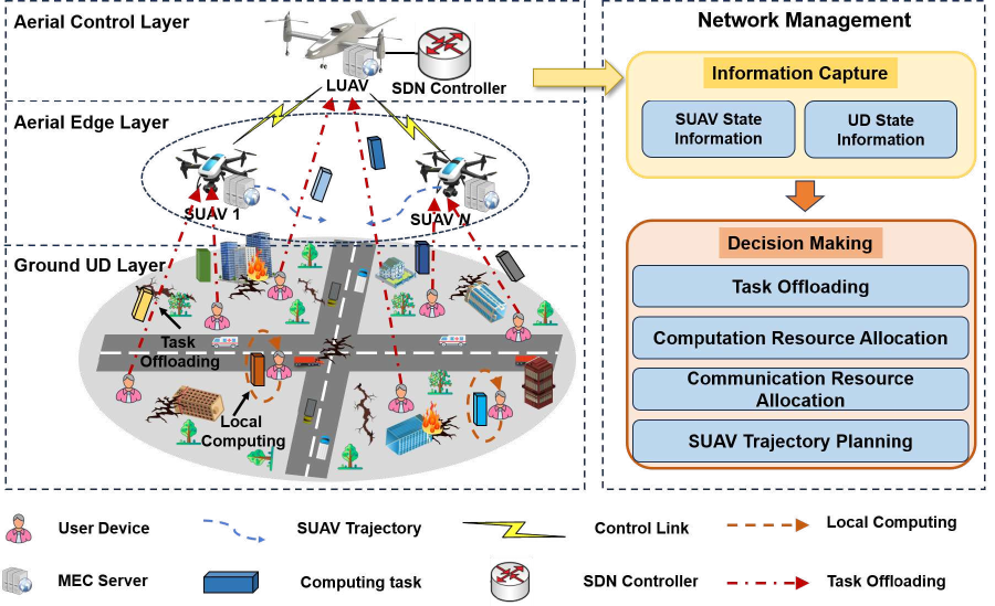
As illustrated in Fig. 1, we consider a hierarchical multiple-UAV-assisted MEC system, where multiple UAVs collaborate to provide aerial edge computing services to ground UDs in a disaster-stricken area. Specifically, in the spatial dimension, the hierarchical system comprises an aerial control layer, an aerial edge layer, and a ground UD layer.
At the aerial control layer, a large rotary-wing UAV (LUAV) is deployed above the service area center to serve as a regional software-defined networking (SDN) controller. It performs the following essential functions: 1) offering wireless communication coverage for UAVs at the aerial edge layer and UDs at the ground UD layer; 2) provisioning reliable edge computing services for UDs; and 3) acting as a regional controller, on which our algorithm runs, to make real-time decisions based on the collected channel state information (CSI), as well as the state information of UDs and UAVs. At the aerial edge layer, a set of small rotary-wing UAVs (SUAVs) is equipped with MEC computing capabilities to provide flexible edge computing services to UDs at the ground user layer. At the ground UD layer, a set of UDs moving within the considered area periodically generates computing tasks with varying requirements.
In the temporal dimension, the system operates in a discrete time slot manner with equal time slots, i.e., , wherein each time slot has a duration of . Here, is chosen to be sufficiently small such that each time slot can be considered as quasi-static. Furthermore, within each time slot, the state information of both UDs and SUAVs, as well as the CSI, are captured and updated. The task offloading, resource allocation and UAV trajectory planning are determined by running our algorithm.
3.1 Basic Models
The basic models define the state information of various entities in the proposed system.
UD Model. We consider that each UD generates one computing task per time slot [30, 34]. For UD , the attributes of the UD at time slot can be characterized as , where denotes the local computing capability of UD . The computing task generated by UD is characterized as at time slot , wherein represents the input data size (in bits), denotes the computation intensity (in cycles/bit), and is the maximum tolerable delay (in s). represents the location coordinates of UD at time slot .
UD Mobility Model. Similar to [35], the mobility of UDs is modeled as a Gauss-Markov mobility model, which is widely employed in cellular communication networks. Specifically, the velocity of UD at time slot can be updated as follows:
| (1) |
where denotes the velocity vector at time slot . represents the memory level, which reflects the temporal-dependent degree. is the asymptotic means of velocity. is the uncorrelated random Gaussian process , where denotes the asymptotic standard deviation of velocity. Therefore, the mobility of UD can be updated as follows:
| (2) |
SUAV Model. Each SUAV is characterized by , wherein and represent the horizontal coordinates and flight height of SUAV at time slot , respectively. Moreover, denotes the total computing resources of SUAV .
SUAV Mobility Model. Similar to [13], we consider that each SUAV flies at a fixed altitude to avoid additional energy consumption caused by frequent ascent and descent. For each SUAV , its trajectory can be expressed as a sequence of optimal positions for each time slot, i.e., . In addition, the trajectory of each SUAV needs to satisfy the following several practical constraints:
| (3a) | |||
| (3b) | |||
| (3c) | |||
where is the initial position of SUAV , denotes the maximum flight speed of SUAV , and denotes the minimum safe distance to avoid collision. Constraint (3a) defines the initial position of each SUAV. Constraint (3b) indicates that the flight distance of each time slot does not exceed the maximum allowable distance, and constraint (3c) ensures the safe flight of SUAVs to avoid collisions.
LUAV Model. LUAV is characterized by , wherein and represent the horizontal coordinates and flight height, respectively. Moreover, denotes the total computing resources.
3.2 Communication Model
The UDs can offload tasks to aerial servers111Note that an aerial server and a UAV will be used interchangeably. via ground-to-air (G2A) links. To mitigate unreliable communication caused by interference, we assume that each aerial server utilizes different frequency band resources to provide edge computing services [33]. Furthermore, the widely used orthogonal frequency-division multiple access (OFDMA) technology can be employed to serve multiple UDs simultaneously [36]. Therefore, there is no communication interference in the system. Assuming UD offloads tasks to server at time slot , the communication rate of the UD can be calculated using Shannon’s formula as follows:
| (4) |
where represents the resource allocation coefficient of UD , denotes the bandwidth resources available to server , is the transmission power of UD , represents the channel gain between UD and server at time slot , and is the noise power.
The probabilistic line-of-sight (LoS) channel model is employed to model the communication between the aerial servers and UDs [37]. First, the LoS probability between server and UD at time slot can be defined as [38]
| (5) |
where and are the constants depending on the propagation environment, denotes the elevation angle, and represents the straight-line distance between server and UD . Similar to [39], the path loss between server and UD can be given by
| (6) | ||||
where represents the carrier frequency of server , and is the speed of light. Moreover, and denote the additional losses for LoS and nLoS links, respectively. Without loss of generality, the channel gain can be calculated as
| (7) |
3.3 Computation Model
For task generated by UD , the task can be processed either locally on the UD or remotely on the aerial servers, which is determined by the offloading decision of the UD. To be more specific, we define a variable to represent the task offloading decision of UD at time slot , where indicates that the task is executed locally, represents that the task is offloaded to the LUAV for execution, and means the task is offloaded to SUAV for execution.
3.3.1 Local Computing Model
If UD processes task locally (i.e., ), the task completion delay and UD energy consumption for local computing are given as follows.
Task Completion Delay. The local completion latency of the task can be calculated as
| (8) |
where represents the computing resources of UD .
UD Energy Consumption. Accordingly, the energy consumption of UD to execute task locally at time slot can be calculated as [27]
| (9) |
where represents the effective switched capacitance coefficient that depends on the hardware architecture [40].
3.3.2 Edge Computing Model
When task is offloaded to aerial server for processing (i.e., ), the server allocates computing resources to perform the task and returns the processing results to the UD. Note that the latency of result feedback has been disregarded when considering the task completion latency, as for most mobile applications, the size of the processing results is typically significantly smaller than the size of the input data.
Task Completion Delay. For edge computing, the task completion delay mainly includes task transmission delay and edge execution delay, which can be calculated as
| (10) |
where denotes the computing resources allocated by server to UD at time slot .
UD Energy Consumption. The task offloading of the UD incurs transmission energy consumption at time slot , which can be calculated as
| (11) |
where represents the transmission power of UD .
SUAV Energy Consumption. If task is offloaded to SUAV , the SUAV incurs computation energy consumption to execute the task, which can be given as [34]
| (12) |
where represents the energy consumption per unit CPU cycle of SUAV . Therefore, the total computational energy consumption of SUAV at time slot can be given as
| (13) |
where is an indicator function defined such that when event is true, and otherwise. Furthermore, the trajectory planning of SUAV incurs corresponding propulsion energy consumption at time slot . Similar to [41, 42], the propulsion power consumption of SUAV at time slot can be expressed as
| (14) | ||||
where represents the velocity of SUAV at time slot , refers to the rotor’s tip speed, and , , , and are the constants described in [43]. Therefore, the energy consumption of SUAV at time slot can be given as
| (15) |
where denotes the propulsion energy consumption at time slot . To guarantee service time, we define the SUAV energy consumption constraint as follows:
| (16) |
where is the energy budget of the SUAV per time slot.
Note that if task is offloaded to server , we ignore the energy consumption of server . This is because server is a large UAV with a more sufficient energy supply, which can provide a longer service time compared to server .
3.4 QoE Evaluation Model
In this paper, we consider that the cost of each UD at time slot consists of the task completion delay and the UD energy consumption, which reflects the QoE of the UD. The completion delay of task can be presented as
| (17) |
Then, the energy consumption of UD can be given as
| (18) |
where and respectively represent the weight coefficients of task completion delay and energy consumption for UD , which can be flexibly set based on the preference of the UD for delay and energy consumption. Clearly, minimizing the cost of UDs is equivalent to maximizing the QoE of UDs.
3.5 Problem Formulation
The objective of this work is to minimize the average cost of all UDs over time (i.e., the time-averaged UD cost), by jointly optimizing the task offloading , computing resource allocation , communication resource allocation , and trajectory planning . Therefore, the problem can be formulated as follows:
| (20) | ||||
| s.t. | (20a) | |||
| (20b) | ||||
| (20c) | ||||
| (20d) | ||||
| (20e) | ||||
| (20f) | ||||
| (20g) | ||||
| (20h) |
Constraint (20a) is the long-term energy consumption constraint of the SUAVs. Constraint (20b) indicates that each UD can only select one strategy as its offloading decision. Constraint (20c) means that the completion delay of edge computing should not exceed the maximum tolerance delay. Constraints (20d) and (20e) imply that the allocated computing resources should be a positive value and not exceed the total amount of computing resources owned by server . Constraints (20f) and (20g) limit the allocation of communication resources.
Challenges. There are two main challenges to obtain the optimal solution of problem P. i) Future-dependent. Optimally solving problem P requires complete future information, e.g., task computing demands and locations of all UDs across all time slots. However, obtaining the future information is very challenging in the considered time-varying scenario. ii) Non-convex and NP-hard. Problem P contains both continuous variables (i.e., resource allocation and trajectory planning ) and binary variables (i.e., task offloading decision ) is a mixed-integer non-linear programming (MINLP) problem, which is non-convex and NP-hard [46, 47].
4 Lyapunov-Based Problem Transformation
In this section, we first explain the motivation behind utilizing the Lyapunov design for online approach. Subsequently, we elaborate on the framework of the proposed Lyapunov-based online approach.
4.1 Motivation
Since problem P is future-dependent, an online approach is necessary to make real-time decisions without foreseeing the future. The Lyapunov-based optimization framework and DRL are two practical tools for designing online approaches. However, DRL typically requires a substantial number of samples to acquire optimal policies and faces challenges in achieving convergence. Furthermore, DRL requires significant computational resources, making it costly in the resource-constrained MEC system. Compared to DRL, the Lyapunov-based optimization framework offers the following advantages:
-
•
Simplicity and Interpretability: The Lyapunov-based optimization framework usually has a simpler structure and are easier to interpret compared to DRL. Furthermore, the Lyapunov-based optimization framework does not introduce additional complexity to the algorithm design.
-
•
Stability: The Lyapunov-based optimization framework provides stability guarantees, which ensures convergence and boundedness of system dynamics.
-
•
Model-free Nature: The Lyapunov-based optimization framework does not require explicit knowledge of the system dynamics, making it suitable for the considered scenario where obtaining future information about system dynamics is challenging and impractical.
Therefore, we adopt the Lyapunov-based optimization framework for online approach design. Furthermore, in the simulation experiments, we compare the proposed Lyapunov-based online approach with DRL-based approaches to verify its suitability for the considered scenarios.
4.2 Problem Transformation
Firstly, to satisfy the SUAV energy consumption constraint (20a), we define two virtual energy queues and to represent the computing energy queue and the propulsion energy queue at time slot based on Lyapunov optimization technique, respectively. We assume that the queues are set as zero at the initial time slot, i.e., and . Therefore, the virtual energy queues can be updated as
| (21) |
where and denote the computation and propulsion energy budgets per slot, respectively, and . Secondly, we define the Lyapunov function , which represents a scalar measure of the queue backlogs, i.e.,
| (22) |
where is the vector of current queue backlogs. Thirdly, we define the conditional Lyapunov drift for time slot as
| (23) |
where is the total cost of all UDs at time slot , and is a parameter to trade off the total cost and the queue stability. Next, we provide an upper bound on the drift-plus-penalty, as stated in Theorem 1.
Theorem 1.
For all and all possible queue backlogs , the drift-plus-penalty is upper bounded as
| (25) | ||||
where is a finite constant.
Proof.
From the inequality , we can know
| (26) |
Then, the following inequality holds, i.e.,
| (27) |
which also applies to queue . Therefore, we can obtain
| (28) | ||||
where is a constant, and and are the upper bounds of computing energy consumption and propulsion energy consumption, respectively. Therefore, we have
| (29) | ||||
According to the Lyapunov optimization framework, we minimize the right-hand side of inequality (25). Therefore, problem P relying on future information is transformed into the real-time optimization problem solvable with only current information, which is given as follows:
| (30) | ||||
| s.t. |
However, problem is still a MINLP problem, with interdependencies among the decision variables. Consequently, the computational burden associated with finding the optimal solution for may not be suitable for real-time decision making. Therefore, we propose a two-stage optimization method that achieves a sub-optimal solution within a polynomial time complexity. Additionally, for the sake of convenience in subsequent discussions, we adopt a notation where the time index is omitted [49].
5 Two-Stage Optimization method
In this section, a two-stage optimization method is proposed to solve the transformed problem . In the first stage, assuming a feasible , we optimize the task offloading and resource allocation . In the second stage, based on the obtained task offloading and resource allocation , we optimize the positions of SUAVs.
5.1 Stage 1: Task Offloading and Resource Allocation
Assuming a feasible and removing irrelevant constant terms, can be transformed into the subproblem P1 to decide task offloading and resource allocation, which is given as follows:
| (31) | ||||
| s.t. |
Problem P1 is still a MINLP problem, and the decisions of task offloading and resource allocation are coupled with each other. Considering that the UAVs are service providers in the considered UAV-assisted MEC system, we prioritize resource allocation strategies for the UAVs. Then, based on the resource allocation strategies, we optimize the offloading decisions of UDs.
5.1.1 Resource Allocation
Given an arbitrary task offloading decision profile of the UDs, the servers decides resource allocation strategies to minimize problem P1. Define and remove irrelevant constant terms, the resource allocation problem can be formulated as
| (32) | ||||
| s.t. | (32a) | |||
| (32b) | ||||
| (32c) | ||||
| (32d) |
where , , and represents the set of UDs that offload tasks to server , which is determined by the offloading decisions .
To solve problem P1.1, we first prove that the problem is a convex optimization problem through Lemma 1. Then, based on Lemma 1, we can obtain the optimal resource allocation by Theorem 2.
Lemma 1.
Problem P1.1 is a convex optimization problem.
Proof.
First, we define to denote the objective function (32). Taking the second-order partial derivative of , we have
| (33) |
Theorem 2.
The optimal resource allocation coefficient, i.e., the solution of problem P1.1, can be given as follows:
| (34) |
Proof.
First, the Lagrange function of Problem P1.1 can be defined as:
| (35) |
where , , and represent the Lagrange multipliers of constraints (32a)-(32d) and are non-negative, respectively. Then, we can obtain the following Karush–Kuhn–Tucker (KKT) conditions.
| Stationarity: | , |
|---|---|
| , | |
| Primal feasibility: | |
| Dual feasibility: | |
| Complementary | |
| slackness: | |
5.1.2 Task Offloading
For UD , let us define as the utility of local computing, as the utility of SUAV-assisted computing, and as the utility of LUAV-assisted computing, which can be given as follows:
| (36) | |||
| (37) | |||
| (38) |
Therefore, we can design the utility function of UD as follows:
| (39) |
According to the optimal resource allocation policy and removing irrelevant constant terms, problem P1 can be reformulated into a task offloading subproblem P1.2 as follows:
| (40) | ||||
| s.t. |
However, the task offloading decision for UD is influenced by not only its individual demand but also the offloading decisions made by other UDs. Given the competitive dynamics inherent in task offloading among UDs, we utilize game theory to address this subproblem.
(1) Game Formulation. We first model the task offloading subproblem as a multi-UDs task offloading game (MUD-TOG). Specifically, the MUD-TOG can be defined as a triplet , which is detailed as follows:
-
•
denotes the set of players, i.e., all UDs.
-
•
denotes the strategy space, wherein is the set of offloading strategies for player , denotes the offloading decision of player , and is the strategy profile.
-
•
represents the utility of player , which maps each strategy profile to a real number.
Every player strives to minimize its utility by selecting an appropriate offloading strategy. Therefore, the MUD-TOG can be described by the following distributed optimization problem mathematically:
| (41) |
where denotes the offloading decisions of the other players except player .
(2) The solution to MUD-TOG. For MUD-TOG, the concept of Nash equilibrium holds great significance as a solution paradigm for predicting the outcome of this game. A Nash equilibrium signifies a strategic profile wherein no individual player possesses the motivation to unilaterally deviate from their current strategy. It can be formally defined as Definition 1.
Definition 1.
If and only if a strategy profile satisfies the following condition, it can be considered as a Nash equilibrium of game
| (42) |
Next, we introduce an important framework called the exact potential game [50] through Definitions 2 and 3, to help us analyze the existence of Nash equilibrium and determine a Nash equilibrium solution for MUD-TOG.
Definition 2.
A game is regarded as an exact potential game if and only if a potential function exists such that
| (43) |
Definition 3.
The FIP implies that a Nash equilibrium can be obtained in a finite number of iterations by any best-response correspondence. Specifically, the best-response correspondence can be formally defined as follows:
Definition 4.
For each player , their best response correspondence corresponds to a set-valued mapping : such that
| (44) |
Therefore, by demonstrating that the MUD-TOG is an exact potential game, we can obtain a Nash equilibrium solution for it. The proof for this is provided in Theorem 3.
Theorem 3.
The MUD-TOG is an exact potential game where the potential function can be given as
| (45) | ||||
where , and .
Proof.
and
| (47) | ||||
Let and , where and . Furthermore, for an arbitrary ordering of UDs, let us introduce the following notation:
where represents the set of UDs who offload tasks to server .
Suppose UD updates its current decision to the decision that leads to a change in its utility function, i.e., . Based on the definition of the potential function, i.e., Definition 2, we demonstrate through the following four cases which also leads to an equal change in the potential function.
Case 1: Suppose that and . According to (45), we can obtain the following conclusion
| (48) | ||||
Case 2: Suppose that and , . According to (45), we can obtain the following conclusion
| (49) | ||||
Case 3: Suppose that and , . According to (45), we can obtain the following conclusion
| (50) | ||||
Case 4: Suppose that and , and . According to (45), we can obtain the following conclusion
| (51) | ||||
Therefore, we can conclude that the MUD-TOG is an exact potential game.
Finally, let us consider the effect of constraint (20c) on the game. We can infer that imposing the constraint may render some strategy profiles infeasible. Suppose is the feasible strategy space, this leads to a new game . Theorem 4 demonstrates that the game is also an exact potential game.
Theorem 4.
is also an exact potential game and has the same potential function as .
Proof.
Since is an exact potential game, the equality (43) holds. Therefore, it remains valid if we restrict and to the new strategy space , which is a subset of . This provides evidence for the validity of this theorem.
The key idea of the MUD-TOG is to utilize the FIP to update the offloading strategies of the players iteratively until a Nash equilibrium is attained, which is outlined in Algorithm 1. The main steps are described as follows. i) All UDs choose local computing for the initial setting (Line 1). ii) Each iteration is partitioned into decision slots (Lines 4-15). Within each decision slot, one UD is chosen to update its offloading decision using the best response correspondence, while the offloading decisions of the remaining UDs remain unchanged. iii) If a lower utility is achieved and constraint (20c) is satisfied, the offloading decision of the UD is updated. Otherwise, the original offloading decision is retained. iv) When no UD changes its offloading decision, the MUD-TOG reaches the Nash equilibrium.
5.2 Stage 2: SUAV Trajectory Planning
Given the optimal task offloading decisions and resource allocation , while removing irrelevant constant terms, problem can be converted into subproblem to decide trajectory planning for SUAVs, which is expressed as follows:
| (52) | |||
where , , , and . Clearly, the objective function in (52) is non-convex with respect to due to the following non-convex terms
| (53) |
Therefore, it is difficult to directly solve problem P2. Next, we transform the objective function into a convex function by introducing slack variables.
For the non-convex term , we introduce the slack variable such that and add the following constraint:
| (54) |
For the non-convex term , we introduce the slack variable such that and add the following constraint:
| (55) |
According to the above-mentioned relaxation transformation, problem P2 can be equivalently transformed as follows:
| (56) | ||||
| s.t. |
where , and .
Note that problem is equivalent to problem , which can be demonstrated by Theorem 3.
Theorem 5.
Problem is equivalent to problem .
Proof.
Suppose is the optimal solution of problem . The following equation holds:
| (57) | ||||
For problem , the optimization objective (56) is convex but constraints (54), (55) and (3c) are still non-convex. Similar to [43, 27], the successive convex approximation (SCA) method is adopted to solve the non-convexity of above constraints, as demonstrated in the following Theorems 6, 7, and 8.
Theorem 6.
For constraint (54), let and given a local point at the -th iteration, we can obtain a global concave lower bound for as
| (58) |
where is defined as
| (59) |
Proof.
Since is a convex quadratic form, the first-order Taylor expansion of at local point is a global concave lower bound.
Theorem 7.
For constraint (55), let and given a local point at the -th iteration, we can obtain a global concave lower bound for as
| (60) |
Proof.
We first consider the function , where , and . The first-derivative of can be calculated as:
| (61) |
Accordingly, the second-order derivative of can be calculated as:
| (62) |
Clearly, since , is a convex function. Therefore, the first-order Taylor expansion of at a local point is a global concave under-estimator of , i.e., the following inequality holds for any
| (63) |
Substituting , and into the inequality (63), we can prove the theorem.
Theorem 8.
For constraint (3c), let and given a local point at the -th iteration, we can obtain a global concave lower bound for as
| (64) |
Proof.
Since the Hessian matrix of is positive semidefinite, is a convex function. Therefore, the first-order Taylor expansion of at local point is a global concave lower bound.
According to Theorems 6, 7, and 8, at the -th iteration, constraints (54), (55), and (3c) can be approximated as:
| (65) | ||||
| (66) | ||||
| (67) |
which are convex. Therefore, problem is converted into a convex optimization problem, which can be efficiently resolved by off-the-shelf optimization tools such as CVX [52]. We summarize the second stage algorithm in Algorithm 2.
5.3 Main Steps of OJTRTA and Performance Analysis
In this section, the main steps of OJTRTA are described in Algorithm 3, and the corresponding analyses are provided in Theorems 9, 10, and 11.
Theorem 9.
Assume that the proposed algorithm results in an optimality gap in solving and denotes the optimal time-averaged UD cost that problem can achieve over all policies given full knowledge of the future computing demands and locations for all UDs, the time-averaged UD cost achieved by the proposed algorithm is bounded by
| (68) |
where is defined in Theorem 1.
Proof.
According to Lemma 4.11 in [48], the T-slot drift-plus-penalty achieved by the proposed algorithm ensures that:
| (69) |
Using the fact that and , and dividing by for the above inequality, we complete the proof of the theorem.
Theorem 10.
The proposed algorithm can satisfy the SUAV energy consumption constraint defined in (16).
Proof.
According to Theorem 4.13 of [48], we can conclude that all virtual queues are rate stable. Therefore, we have
| (70) |
Using the sample path property (Lemma 2.1 of [48]), we have
| (71) |
Theorem 11.
The proposed OJTRTA has a polynomial worst-case complexity in each time slot, i.e., , where represents the number of iterations required for Algorithm 1 to converge to the Nash equilibrium, denotes the number of UDs and is the accuracy of SCA for solving problem .
Proof.
OJTRTA contains two phases in each time slot, i.e., Algorithm 1 and Algorithm 2. In Algorithm 1, assuming that the outer iteration (i.e., Lines ) converges after iterations, the computational complexity can be calculated as . In Algorithm 2, problem can contain at most variables and constraints. According to the analysis in [30], the number of iterations required is , where is the accuracy of SCA. Therefore, the computational complexity of Algorithm 2 can be calculated as , which is equivalent to . As a result, the computational complexity of OJTRTA is in the worst case.
Accordingly, it is proven that the proposed approach can effectively guarantee the performance of the system and meet the SUAV energy consumption constraint with the feasible computational complexity.
6 Simulation Results
In this section, we conduct simulation experiments to validate the effectiveness of the proposed OJTRTA.
6.1 Simulation Setup
We first describe the settings related to the simulation experiments, including the scenario, parameters, comparative approaches, and performance evaluation metrics.
6.1.1 Scenario
We consider a multiple-UAV-assisted MEC system, where one LUAV and four SUAVs are deployed to collaboratively provide edge computing services for ground UDs in a rectangular service area. The system timeline is divided into equal time slots, and the duration of each time slot is set to .
6.1.2 Parameters
| Symbol | Meaning | Value (Unit) |
|---|---|---|
| Task size | Mb | |
| Computation intensity of tasks | cycles/bit | |
| Maximum tolerable delay of tasks | s | |
| Memory level of velocity | ||
| the velocity of UD | m/s [43] | |
| The asymptotic standard deviation of velocity | [43] | |
| Computation resources of SUAVs | GHz | |
| Maximum flight speed of SUAVs | m/s [43] | |
| Minimum safety distance | m | |
| Computation resources of LUAV | GHz | |
| Bandwidth of MEC server |
MHz ,
MHz |
|
| Transmission power of UD | dBm | |
| Noise power | dBm | |
| , | Parameters for LoS probability | 10, 0.6 [53, 41] |
| Additional losses for LoS and nLoS links | 1.0 dB, 20 dB [53] | |
| CPU parameters | ||
| Energy consumption per unit CPU cycle of SUAVs | J [34] | |
| , , , | UAV propulsion power consumption parameters | 80, 22, 263.4, 0.0092 [43] |
| Energy budget per time slot for SUAV | 220 J | |
| Tip speed of the rotor | 120 m/s | |
| , | The weight coefficients of task completion delay and energy consumption for UD | 0.7, 0.3 |
For the LUAV, the fixed horizontal position and altitude are set as and , respectively. For the SUAVs, the fixed altitude is set as , and the initial positions are set as , , , and , respectively. For the UDs, the computing capacity of each UD is randomly taken from . The default values for the remaining parameters can be found in Table II.
6.1.3 Comparative Approaches
To validate the effectiveness of the proposed OJTRTA, this work compares OJTRTA with the following approaches.
-
•
Entire offloading (EO) [54]: All UDs offload their tasks to aerial servers for execution. This approach does not consider local computing.
-
•
Equal resource allocation (ERA) [55]: The communication and computing resources of each edge server are equally allocated to the requested UDs.
-
•
Fixed location deployment (FLP) [30]: The SUAV are deployed at fixed positions within the service area to provide edge computing services.
-
•
Only consider QoE (OCQ) [34]: Ignoring the SUAV energy consumption constraint, all decisions are made only to minimize the time-averaged UD cost.
-
•
DDPG-based joint optimization (DDPG-JO) [32]: The decisions of task offloading, resource allocation, and trajectory planning are decided by the DDPG algorithm.
-
•
PPO-based joint optimization (PPO-JO) [33]: The decisions of task offloading, resource allocation, and trajectory planning are determined by the PPO algorithm.
6.1.4 Performance Metrics
We evaluate the overall performance of the proposed approach based on the following performance metrics. 1) Time-averaged UD cost , which represents the average cumulative cost of all UDs per unit time. 2) Average task completion latency , which indicates the average latency for completing a task. 3) Cumulative UD energy consumption , which signifies the cumulative energy consumption of UDs over the system timeline. 4) Time-averaged SUAV energy consumption , which means the average energy consumption of each SUAV per unit time.
6.2 Evaluation Results
In this section, we first evaluate the system performance of the proposed OJTRTA over time with default parameters. Subsequently, we compare the impacts of different parameters on the performance of the proposed OJTRTA and the benchmark approaches.
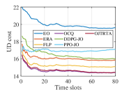
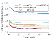
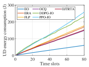
6.2.1 Online Offloading Performance Evaluation
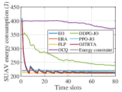
Figs. 2(a), 2(b), 2(c) and 2(d) show the dynamics of time-averaged UD cost, average task completion latency, cumulative UD energy consumption, and time-averaged SUAV energy consumption, respectively among the seven approaches. It can be observed that the time-averaged UD cost exhibits some fluctuations over time. This is primarily attributed to the time-varying computational demands of UDs. Additionally, OCQ slightly outperforms the proposed OJTRTA in terms of time-averaged UD cost, average task completion latency, and overall UD energy consumption. This is because OCQ does not consider the energy constraints of SUAVs and thus consumes more SUAV energy. Furthermore, the proposed OJTRTA outperforms EO, ERA, and FLP in terms of time-averaged UD cost and average task completion latency. This is due to the combined local and edge offloading strategy, optimal resource allocation strategy, and trajectory planning strategy of OJTRTA. Moreover, compared to DRL-based approaches, i.e., DDPG-JO and PPO-JO, the proposed OJTRTA exhibits significant advantages in terms of time-averaged UD cost, average task completion delay, and cumulative UD energy consumption. This further exemplifies the effectiveness of the proposed approach. Finally, as shown in Fig. 2(d), the proposed OJTRTA ensures long-term energy constraints satisfaction for SUAVs under the real-time guidance of the Lyapunov-based energy queue, which is consistent with the analysis in Theorem 10. In conclusion, the set of simulation results demonstrates the effectiveness of the proposed approach in achieving better overall performance while satisfying the long-term energy consumption constraint of SUAVs.
6.2.2 Impact of Parameters
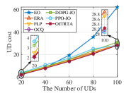
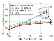
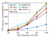
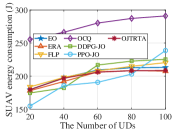
Impact of UD Numbers. Figs. 3(a), 3(b), 3(c), and 3(d) illustrate the impact of varying numbers of UDs on the time-averaged UD cost, average task completion delay, cumulative UD energy consumption, and time-averaged SUAV energy consumption, respectively. It can be observed that the time-averaged UD cost, cumulative UD energy consumption and time-averaged SUAV energy consumption of all approaches show an upward trend as the number of UDs increases, since more computation tasks need to be processed. Furthermore, as the number of UDs increases, EO exhibits the poorest performance in terms of average task completion latency, while demonstrating optimal performance in cumulative UD energy consumption. This is primarily due to EO offloading all tasks to edge servers, resulting in lower UD energy consumption but higher server loads. Additionally, compared to the proposed approach, FLP shows inferior performance in terms of average task completion latency and cumulative UD energy consumption. This highlights the importance of optimizing the trajectory of UAVs. Besides, when the number of UDs reaches 100, OCQ and PPO-JO slightly outperform the proposed approach in terms of time-averaged UD cost. This can be attributed to the fact that OCQ and PPO-JO do not consider SUAV energy consumption constraints. As shown in Fig. 3(d), OCQ and PPO-JO exhibit higher time-averaged SUAV energy consumption.
Lastly, the proposed OJTRTA approach demonstrates superior performance in terms of time-averaged UD cost and average task completion latency compared to other approaches, while also exhibiting favorable performance in terms of cumulative UD energy consumption and time-averaged SUAV energy consumption. Specifically, compared with EO, ERA, FLP, and DDPG-JO, the proposed approach can respectively reduce the time-averaged UD cost by 54.7%, 2.3%, 1.7%, 8.8% and can respectively reduce the average task completion latency 58.1%, 0.4%, 2.6%, 4.2% in the relative dense scenario (). In conclusion, the set of simulation results indicates that the proposed OJTRTA has better scalability with an increasing number of UDs.
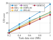
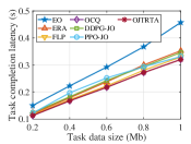
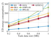
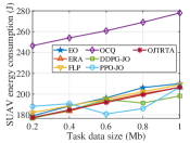
Impact of Task Data Size. Figs. 4(a), 4(b), 4(c), and 4(d) show the impact of task data sizes on the time-averaged UD cost, average task completion latency, cumulative UD energy consumption, and time-averaged SUAV energy consumption. It can be seen that with the increase in task data sizes, there is an upward trend in terms of the time-averaged UD cost, average task completion latency, cumulative UD energy consumption, and time-averaged SUAV energy consumption. This is expected as the larger task data size leads to higher overheads on computing, communication, and energy consumption for UDs and UAVs. In addition, EO exhibits a significant growth trend in terms of the time-averaged UD cost and average task completion latency compared to other approaches. This is due to the increased competition for the limited computational and communication resources of aerial servers caused by the entire offloading of EO as the task data size increases.
Finally, compared with EO, ERA, FLP, DDPG-JO and PPO-JO, the proposed OJTRTA achieves performance improvements of approximately 27.6%, 9.1%, 3.4%, 9.3%, and 6.8% in terms of time-averaged UD cost, as well as 30%, 9.2%, 2.8%, 7.5%, and 3.3% in terms of average task completion latency when the task data size reaches 1 Mb. The set of simulation results indicates that the proposed OJTRTA is able to adapt to the heavy-loaded scenarios with overall superior performances.
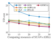
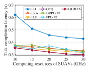
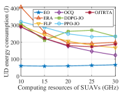
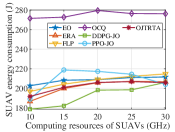
Impact of Computing Resources of SUAVs. Figs. 5(a), 5(b), 5(c), and 5(d) depict the impact of different SUAV computing resources on the time-averaged UD cost, average task completion delay, cumulative UD energy consumption, and time-averaged SUAV energy consumption. It can be observed that with the increase of SUAV computing resources, all approaches show a decreasing trend in terms of the time-averaged UD cost and average task completion latency, and EO and OJTRTA demonstrate gradually decreasing performance improvements. The reasons can be explained as follows. The increase of SUAV computational resources provides more computing resource allocation for task execution, reducing the task execution latency. However, as SUAV computing resources further increase, communication resources and the energy constraints of SUAV become bottlenecks that limit the improvement of system performance. Furthermore, EO maintains nearly constant performance in terms of the cumulative UD energy consumption regardless of the variations in the computing resources of SUAVs. This is mainly because the entire offloading of EO primarily incurs transmission energy consumption for UDs, which is independent of the computing resources of SUAVs.
Finally, OJTRTA outperforms EO, ERA, FLP, DDPG-JO and PPO-JO in terms of the time-averaged UD cost and average task completion delay, which illustrates the proposed approach enables sustainable utilization of computing resources and prevents resource over-utilization.
6.2.3 UAV Trajectory Planning
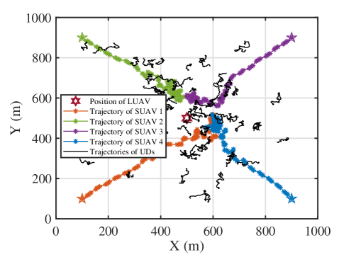
Fig. 6 shows the mobility of UDs and the flight trajectories of SUAVs controlled by the proposed OJTRTA approach. It can be observed that the flight trajectories of SUAVs are in accordance with intuition. Specifically, SUAVs tend to fly towards areas with dense UDs to serve a greater number of UDs and provide improved communication conditions, thereby enhancing the QoE of the serviced UDs. After reaching the dense UD area, SUAVs adjust their positions to accommodate the dynamic computing demands of the UDs. Besides, it is worth noting that the proposed approach incorporates collision avoidance, effectively ensuring the safe flight of SUAVs in dense UD areas. In conclusion, the simulation results demonstrate that the trajectory control of the proposed OJTRTA approach can effectively regulate the trajectories of SUAVs according to the dynamic computing requirements to improve the QoE of UDs.
7 Conclusion
In this work, we studied the task offloading, resource allocation, and UAV trajectory planning in an energy-constrained UAV-enabled MEC system. A JTRTOP was formulated to maximize the QoE of all UDs while satisfying the UAV energy consumption constraint. Since the JTRTOP is future-dependent and NP-hard, we proposed the OJTRTA to solve the problem. Specifically, the future-dependent JTRTOP was first transformed into the PROP by using Lyapunov optimization methods. Furthermore, a two-stage optimization algorithm was proposed to solve the PROP. Simulation results show that OJTRTA outperforms the comparative approaches in terms of time-averaged UD cost while meeting the SUAV energy consumption constraint. Furthermore, JTRTOP exhibits superior adaptability in heavy-loaded scenarios and demonstrates good scalability with an increasing number of MDs. In the future, we will integrate satellite networks into our work to explore the integration of space-air-ground MEC networks.
References
- [1] L. He, G. Sun, Z. Sun, P. Wang, J. Li, S. Liang, and D. Niyato, “An online joint optimization approach for QoE maximization in UAV-enabled mobile edge computing,” in Proc. IEEE INFOCOM, 2024.
- [2] B. Hou, S. Yang, F. A. Kuipers, L. Jiao, and X. Fu, “EAVS: Edge-assisted adaptive video streaming with fine-grained serverless pipelines,” in Proc. IEEE INFOCOM, 2023, pp. 1–10.
- [3] L. Liu, H. Li, and M. Gruteser, “Edge assisted real-time object detection for mobile augmented reality,” in Proc. ACM MobiCom, 2019, pp. 25:1–25:16.
- [4] W. Shi, J. Cao, Q. Zhang, Y. Li, and L. Xu, “Edge computing: Vision and challenges,” IEEE Internet Things J., vol. 3, no. 5, pp. 637–646, Oct. 2016.
- [5] A. Hekmati, P. Teymoori, T. D. Todd, D. Zhao, and G. Karakostas, “Optimal mobile computation offloading with hard deadline constraints,” IEEE Trans. Mob. Comput., vol. 19, no. 9, pp. 2160–2173, Sep. 2020.
- [6] Y. Mao, C. You, J. Zhang, K. Huang, and K. B. Letaief, “A survey on mobile edge computing: The communication perspective,” IEEE Commun. Surv. Tutorials, vol. 19, no. 4, pp. 2322–2358, Fourthquarter 2017.
- [7] J. Li, G. Sun, L. Duan, and Q. Wu, “Multi-objective optimization for UAV swarm-assisted IoT with virtual antenna arrays,” IEEE Trans. Mob. Comput., vol. 23, no. 5, pp. 4890–4907, May 2024.
- [8] J. Li, G. Sun, H. Kang, A. Wang, S. Liang, Y. Liu, and Y. Zhang, “Multi-objective optimization approaches for physical layer secure communications based on collaborative beamforming in UAV networks,” IEEE/ACM Trans. Netw., vol. 31, no. 4, pp. 1902–1917, Aug. 2023.
- [9] P. A. Apostolopoulos, G. Fragkos, E. Tsiropoulou, and S. Papavassiliou, “Data offloading in UAV-assisted multi-access edge computing systems under resource uncertainty,” IEEE Trans. Mob. Comput., vol. 22, no. 1, pp. 175–190, Jan. 2023.
- [10] P. Vamvakas, E. Tsiropoulou, and S. Papavassiliou, “On the prospect of UAV-assisted communications paradigm in public safety networks,” in Proc. IEEE INFOCOM, 2019, pp. 762–767.
- [11] N. Lin, H. Tang, L. Zhao, S. Wan, A. Hawbani, and M. Guizani, “A PDDQNLP algorithm for energy efficient computation offloading in UAV-assisted MEC,” IEEE Trans. Wirel. Commun., vol. 22, no. 12, pp. 8876–8890, Dec. 2023.
- [12] Z. Yu, Y. Gong, S. Gong, and Y. Guo, “Joint task offloading and resource allocation in UAV-enabled mobile edge computing,” IEEE Internet Things J., vol. 7, no. 4, pp. 3147–3159, Apr. 2020.
- [13] B. Li, R. Yang, L. Liu, J. Wang, N. Zhang, and M. Dong, “Robust computation offloading and trajectory optimization for multi-UAV-assisted MEC: A multiagent DRL approach,” IEEE Internet Things J., vol. 11, no. 3, pp. 4775–4786, Feb. 2024.
- [14] S. Goudarzi, S. A. Soleymani, W. Wang, and P. Xiao, “UAV-enabled mobile edge computing for resource allocation using cooperative evolutionary computation,” IEEE Trans. Aerosp. Electron. Syst., vol. 59, no. 5, pp. 5134–5147, Oct. 2023.
- [15] Z. Bai, Y. Lin, Y. Cao, and W. Wang, “Delay-aware cooperative task offloading for multi-UAV enabled edge-cloud computing,” IEEE Trans. Mob. Comput., vol. 23, no. 2, pp. 1034–1049, Feb. 2024.
- [16] Q. Luan, H. Cui, L. Zhang, and Z. Lv, “A hierarchical hybrid subtask scheduling algorithm in UAV-assisted MEC emergency network,” IEEE Internet Things J., vol. 9, no. 14, pp. 12 737–12 753, Jul. 2022.
- [17] C. Deng, X. Fang, and X. Wang, “UAV-enabled mobile-edge computing for AI applications: Joint model decision, resource allocation, and trajectory optimization,” IEEE Internet Things J., vol. 10, no. 7, pp. 5662–5675, Apr. 2023.
- [18] N. N. Ei, M. Alsenwi, Y. K. Tun, Z. Han, and C. S. Hong, “Energy-efficient resource allocation in multi-UAV-assisted two-stage edge computing for beyond 5G networks,” IEEE Trans. Intell. Transp. Syst., vol. 23, no. 9, pp. 16 421–16 432, Sep. 2022.
- [19] B. Liu, Y. Wan, F. Zhou, Q. Wu, and R. Q. Hu, “Resource allocation and trajectory design for MISO UAV-assisted MEC networks,” IEEE Trans. Veh. Technol., vol. 71, no. 5, pp. 4933–4948, May 2022.
- [20] S. Tong, Y. Liu, J. V. Misic, X. Chang, Z. Zhang, and C. Wang, “Joint task offloading and resource allocation for fog-based intelligent transportation systems: A UAV-enabled multi-hop collaboration paradigm,” IEEE Trans. Intell. Transp. Syst., vol. 24, no. 11, pp. 12 933–12 948, Nov. 2023.
- [21] H. Hao, C. Xu, W. Zhang, S. Yang, and G.-M. Muntean, “Joint task offloading, resource allocation, and trajectory design for multi-UAV cooperative edge computing with task priority,” IEEE Trans. Mob. Comput., pp. 1–16, Early Access, 2024, doi:10.1109/TMC.2024.3350078.
- [22] X. Chen, Y. Bi, G. Han, D. Zhang, M. Liu, H. Shi, H. Zhao, and F. Li, “Distributed computation offloading and trajectory optimization in multi-UAV-enabled edge computing,” IEEE Internet Things J., vol. 9, no. 20, pp. 20 096–20 110, Oct. 2022.
- [23] F. Song, H. Xing, X. Wang, S. Luo, P. Dai, Z. Xiao, and B. Zhao, “Evolutionary multi-objective reinforcement learning based trajectory control and task offloading in UAV-assisted mobile edge computing,” IEEE Trans. Mob. Comput., vol. 22, no. 12, pp. 7387–7405, Dec. 2023.
- [24] F. Pervez, A. Sultana, C. Yang, and L. Zhao, “Energy and latency efficient joint communication and computation optimization in a multi-UAV-assisted MEC network,” IEEE Trans. Wirel. Commun., vol. 23, no. 3, pp. 1728–1741, Mar. 2024.
- [25] A. M. Seid, A. Erbad, H. N. Abishu, A. Albaseer, M. Abdallah, and M. Guizani, “Multiagent federated reinforcement learning for resource allocation in UAV-enabled internet of medical things networks,” IEEE Internet Things J., vol. 10, no. 22, pp. 19 695–19 711, Nov. 2023.
- [26] Y. Xu, T. Zhang, Y. Liu, D. Yang, L. Xiao, and M. Tao, “UAV-assisted MEC networks with aerial and ground cooperation,” IEEE Trans. Wirel. Commun., vol. 20, no. 12, pp. 7712–7727, Dec. 2021.
- [27] X. Zhang, J. Zhang, J. Xiong, L. Zhou, and J. Wei, “Energy-efficient multi-UAV-enabled multiaccess edge computing incorporating NOMA,” IEEE Internet Things J., vol. 7, no. 6, pp. 5613–5627, Jun. 2020.
- [28] Q. Hu, Y. Cai, G. Yu, Z. Qin, M. Zhao, and G. Y. Li, “Joint offloading and trajectory design for UAV-enabled mobile edge computing systems,” IEEE Internet Things J., vol. 6, no. 2, pp. 1879–1892, Apr. 2019.
- [29] R. Zhou, X. Wu, H. Tan, and R. Zhang, “Two time-scale joint service caching and task offloading for UAV-assisted mobile edge computing,” in Proc. IEEE INFOCOM, 2022, pp. 1189–1198.
- [30] L. Wang, K. Wang, C. Pan, W. Xu, N. Aslam, and A. Nallanathan, “Deep reinforcement learning based dynamic trajectory control for UAV-assisted mobile edge computing,” IEEE Trans. Mob. Comput., vol. 21, no. 10, pp. 3536–3550, Oct. 2022.
- [31] L. T. Hoang, C. T. Nguyen, and A. T. Pham, “Deep reinforcement learning-based online resource management for UAV-assisted edge computing with dual connectivity,” IEEE/ACM Trans. Netw., vol. 31, no. 6, pp. 2761–2776, Dec. 2023.
- [32] J. Miao, S. Bai, S. Mumtaz, Q. Zhang, and J. Mu, “Utility-oriented optimization for video streaming in UAV-aided MEC network: A DRL approach,” IEEE Trans. Green Commun. Netw., vol. 8, no. 2, pp. 878–889, Jun. 2024.
- [33] W. Xu, T. Zhang, X. Mu, Y. Liu, and Y. Wang, “Trajectory planning and resource allocation for multi-UAV cooperative computation,” IEEE Trans. Wirel. Commun., pp. 1–1, Early Access, 2024, doi: 10.1109/TCOMM.2024.3361536.
- [34] H. Jiang, X. Dai, Z. Xiao, and A. Iyengar, “Joint task offloading and resource allocation for energy-constrained mobile edge computing,” IEEE Trans. Mob. Comput., vol. 22, no. 7, pp. 4000–4015, Jul. 2023.
- [35] B. Liang and Z. J. Haas, “Predictive distance-based mobility management for PCS networks,” in Proc. of IEEE INFOCOM, 1999, pp. 1377–1384.
- [36] Z. Wei, Y. Cai, Z. Sun, D. W. K. Ng, J. Yuan, M. Zhou, and L. Sun, “Sum-rate maximization for IRS-assisted UAV OFDMA communication systems,” IEEE Trans. Wirel. Commun., vol. 20, no. 4, pp. 2530–2550, Apr. 2021.
- [37] L. Zhang, Z. Zhang, L. Min, C. Tang, H. Zhang, Y. Wang, and P. Cai, “Task offloading and trajectory control for UAV-assisted mobile edge computing using deep reinforcement learning,” IEEE Access, vol. 9, pp. 53 708–53 719, Apr. 2021.
- [38] G. Sun, X. Zheng, Z. Sun, Q. Wu, J. Li, Y. Liu, and V. C. M. Leung, “UAV-enabled secure communications via collaborative beamforming with imperfect eavesdropper information,” IEEE Trans. Mob. Comput., vol. 23, no. 4, pp. 3291–3308, Apr. 2024.
- [39] Y. Chen, K. Li, Y. Wu, J. Huang, and L. Zhao, “Energy efficient task offloading and resource allocation in air-ground integrated MEC systems: A distributed online approach,” IEEE Trans. Mob. Comput., pp. 1–14, Early Access, 2023, doi: 10.1109/TMC.2023.3346431.
- [40] Y. Pan, C. Pan, K. Wang, H. Zhu, and J. Wang, “Cost minimization for cooperative computation framework in MEC networks,” IEEE Trans. Wirel. Commun., vol. 20, no. 6, pp. 3670–3684, Jun. 2021.
- [41] Y. Zeng, J. Xu, and R. Zhang, “Energy minimization for wireless communication with rotary-wing UAV,” IEEE Trans. Wirel. Commun., vol. 18, no. 4, pp. 2329–2345, Apr. 2019.
- [42] H. Pan, Y. Liu, G. Sun, J. Fan, S. Liang, and C. Yuen, “Joint power and 3D trajectory optimization for UAV-enabled wireless powered communication networks with obstacles,” IEEE Trans. Commun., vol. 71, no. 4, pp. 2364–2380, Apr. 2023.
- [43] Z. Yang, S. Bi, and Y. A. Zhang, “Online trajectory and resource optimization for stochastic UAV-enabled MEC systems,” IEEE Trans. Wirel. Commun., vol. 21, no. 7, pp. 5629–5643, Jul. 2022.
- [44] Y. Chen, J. Zhao, Y. Wu, J. Huang, and X. Shen, “QoE-aware decentralized task offloading and resource allocation for end-edge-cloud systems: A game-theoretical approach,” IEEE Trans. Mob. Comput., vol. 23, no. 1, pp. 769–784, Jan. 2024.
- [45] Y. Ding, K. Li, C. Liu, and K. Li, “A potential game theoretic approach to computation offloading strategy optimization in end-edge-cloud computing,” IEEE Trans. Parallel Distributed Syst., vol. 33, no. 6, pp. 1503–1519, Jun. 2022.
- [46] S. Boyd, S. P. Boyd, and L. Vandenberghe, Convex optimization. Cambridge university press, 2004.
- [47] P. Belotti, C. Kirches, S. Leyffer, J. Linderoth, J. Luedtke, and A. Mahajan, “Mixed-integer nonlinear optimization,” Acta Numerica, vol. 22, pp. 1–131, Apr. 2013.
- [48] M. J. Neely, Stochastic Network Optimization with Application to Communication and Queueing Systems, ser. Synthesis Lect. Commun. Netw. Morgan & Claypool Publishers, 2010.
- [49] G. Cui, Q. He, X. Xia, F. Chen, F. Dong, H. Jin, and Y. Yang, “OL-EUA: Online user allocation for NOMA-based mobile edge computing,” IEEE Trans. Mob. Comput., vol. 22, no. 4, pp. 2295–2306, Apr. 2023.
- [50] D. Monderer and L. S. Shapley, “Potential Games,” Games Econ. Behav., vol. 14, no. 1, pp. 124–143, 1996.
- [51] D. L. Quang, Y. H. Chew, and B. H. Soong, “Potential games,” Springer International Publishing, 2016.
- [52] M. Grant and S. Boyd, “CVX: Matlab software for disciplined convex programming, version 2.1,” http://cvxr.com/cvx, Mar. 2014.
- [53] A. Al-Hourani, K. Sithamparanathan, and S. Lardner, “Optimal LAP altitude for maximum coverage,” IEEE Wirel. Commun. Lett., vol. 3, no. 6, pp. 569–572, Dec. 2014.
- [54] L. Zhang and N. Ansari, “Latency-aware IoT service provisioning in UAV-aided mobile-edge computing networks,” IEEE Internet Things J., vol. 7, no. 10, pp. 10 573–10 580, Oct. 2020.
- [55] S. Josilo and G. Dán, “Selfish decentralized computation offloading for mobile cloud computing in dense wireless networks,” IEEE Trans. Mob. Comput., vol. 18, no. 1, pp. 207–220, Jan. 2019.
![[Uncaptioned image]](/html/2406.11918/assets/x19.png) |
Long He received a BS degree in Computer Science and Technology from Chengdu University of Technology, Sichuan, China, in 2019. He is currently working toward the PhD degree in Computer Science and Technology at Jilin University, Changchun, China. His research interests include vehicular networks and edge computing. |
![[Uncaptioned image]](/html/2406.11918/assets/x20.png) |
Geng Sun (Senior Member, IEEE) received the B.S. degree in communication engineering from Dalian Polytechnic University, and the Ph.D. degree in computer science and technology from Jilin University, in 2011 and 2018, respectively. He was a Visiting Researcher with the School of Electrical and Computer Engineering, Georgia Institute of Technology, USA. He is an Associate Professor in College of Computer Science and Technology at Jilin University, and his research interests include wireless networks, UAV communications, collaborative beamforming and optimizations. |
![[Uncaptioned image]](/html/2406.11918/assets/x21.png) |
Zemin Sun received a BS degree in Software Engineering, an MS degree and a Ph.D degree in Computer Science and Technology from Jilin University, Changchun, China, in 2015, 2018, and 2022, respectively. Her research interests include vehicular networks, edge computing, and game theory. |
![[Uncaptioned image]](/html/2406.11918/assets/x22.png) |
Qingqing Wu (Senior Member, IEEE) received the B.Eng. and the Ph.D. degrees in Electronic Engineering from South China University of Technology and Shanghai Jiao Tong University (SJTU) in 2012 and 2016, respectively. From 2016 to 2020, he was a Research Fellow in the Department of Electrical and Computer Engineering at National University of Singapore. He is currently an Associate Professor with Shanghai Jiao Tong University. His current research interest includes intelligent reflecting surface (IRS), unmanned aerial vehicle (UAV) communications, and MIMO transceiver design. He has coauthored more than 100 IEEE journal papers with 26 ESI highly cited papers and 8 ESI hot papers, which have received more than 18,000 Google citations. He was listed as the Clarivate ESI Highly Cited Researcher in 2022 and 2021, the Most Influential Scholar Award in AI-2000 by Aminer in 2021 and World’s Top 2% Scientist by Stanford University in 2020 and 2021. |
![[Uncaptioned image]](/html/2406.11918/assets/x23.png) |
Jiawen Kang (Senior Member, IEEE) received the Ph.D. degree from Guangdong University of Technology, China, in 2018. He was a Post-Doctoral Researcher with Nanyang Technological University, Singapore, from 2018 to 2021. He is currently a Professor with Guangdong University of Technology. His main research interests include blockchain, security, and privacy protection in wireless communications and networking. |
![[Uncaptioned image]](/html/2406.11918/assets/x24.png) |
Dusit Niyato (Fellow, IEEE) received the B.Eng. degree from the King Mongkuts Institute of Technology Ladkrabang (KMITL), Thailand, in 1999, and the Ph.D. degree in electrical and computer engineering from the University of Manitoba, Canada, in 2008. He is currently a Professor with the School of Computer Science and Engineering, Nanyang Technological University, Singapore. His research interests include the Internet of Things (IoT), machine learning, and incentive mechanism design. |
![[Uncaptioned image]](/html/2406.11918/assets/x25.png) |
Zhu Han (Fellow, IEEE) received the B.S. degree in electronic engineering from Tsinghua University, in 1997, and the M.S. and Ph.D. degrees in electrical and computer engineering from the University of Maryland, College Park, in 1999 and 2003, respectively. Currently, he is a John and Rebecca Moores Professor in the Electrical and Computer Engineering Department as well as in the Computer Science Department at the University of Houston, Texas. Dr. Han’s main research targets on the novel game-theory related concepts critical to enabling efficient and distributive use of wireless networks with limited resources. His other research interests include wireless resource allocation and management, wireless communications and networking, quantum computing, data science, smart grid, carbon neutralization, security and privacy. Dr. Han received an NSF Career Award in 2010, the Fred W. Ellersick Prize of the IEEE Communication Society in 2011, the EURASIP Best Paper Award for the Journal on Advances in Signal Processing in 2015, IEEE Leonard G. Abraham Prize in the field of Communications Systems (best paper award in IEEE JSAC) in 2016, IEEE Vehicular Technology Society 2022 Best Land Transportation Paper Award, and several best paper awards in IEEE conferences. Dr. Han was an IEEE Communications Society Distinguished Lecturer from 2015 to 2018 and ACM Distinguished Speaker from 2022 to 2025, AAAS fellow since 2019, and ACM Fellow since 2024. Dr. Han is a 1% highly cited researcher since 2017 according to Web of Science. Dr. Han is also the winner of the 2021 IEEE Kiyo Tomiyasu Award (an IEEE Field Award), for outstanding early to mid-career contributions to technologies holding the promise of innovative applications, with the following citation: “for contributions to game theory and distributed management of autonomous communication networks.” |
![[Uncaptioned image]](/html/2406.11918/assets/x26.png) |
Victor C. M. Leung (Life Fellow, IEEE) is a Distinguished Professor of computer science and software engineering with Shenzhen University, China. He is also an Emeritus Professor of electrial and computer engineering and the Director of the Laboratory for Wireless Networks and Mobile Systems at the University of British Columbia (UBC). His research is in the broad areas of wireless networks and mobile systems. He has co-authored more than 1300 journal/conference papers and book chapters. Dr. Leung is serving on the editorial boards of IEEE Transactions on Green Communications and Networking, IEEE Transactions on Cloud Computing, IEEE Access, and several other journals. He received the IEEE Vancouver Section Centennial Award, 2011 UBC Killam Research Prize, 2017 Canadian Award for Telecommunications Research, and 2018 IEEE TCGCC Distinguished Technical Achievement Recognition Award. He co-authored papers that won the 2017 IEEE ComSoc Fred W. Ellersick Prize, 2017 IEEE Systems Journal Best Paper Award, 2018 IEEE CSIM Best Journal Paper Award, and 2019 IEEE TCGCC Best Journal Paper Award. He is a Life Fellow of IEEE, and a Fellow of the Royal Society of Canada, Canadian Academy of Engineering, and Engineering Institute of Canada. He is named in the current Clarivate Analytics list of Highly Cited Researchers. |