Towards Better Benchmark Datasets
for Inductive Knowledge Graph Completion
Abstract
Knowledge Graph Completion (KGC) attempts to predict missing facts in a Knowledge Graph (KG). Recently, there’s been an increased focus on designing KGC methods that can excel in the inductive setting, where a portion or all of the entities and relations seen in inference are unobserved during training. Numerous benchmark datasets have been proposed for inductive KGC, all of which are subsets of existing KGs used for transductive KGC. However, we find that the current procedure for constructing inductive KGC datasets inadvertently creates a shortcut that can be exploited even while disregarding the relational information. Specifically, we observe that the Personalized PageRank (PPR) score can achieve strong or near SOTA performance on most inductive datasets. In this paper, we study the root cause of this problem. Using these insights, we propose an alternative strategy for constructing inductive KGC datasets that helps mitigate the PPR shortcut. We then benchmark multiple popular methods using the newly constructed datasets and analyze their performance. The new benchmark datasets help promote a better understanding of the capabilities and challenges of inductive KGC by removing any shortcuts that obfuscate performance.
1 Introduction
Knowledge Graph Completion (KGC) attempts to predict unseen facts on an existing knowledge graph (KG). KGC has numerous applications including drug discovery [1], personalized medicine [2], and recommendations [3]. Traditionally, most research on KGC has focused on the transductive setting, where the same entities and relations are seen during training and testing. Most methods [4, 5, 6] generally focus on learning embeddings for all entities and relations to facilitate the prediction of new facts.
In recent years, interest in KGC has shifted towards designing methods that can generalize to new entities or relations not seen during training. This task, known as “inductive KGC”, requires a method to train on a graph and perform inference on a different graph , where the inference graph contains either new entities, relations, or both. Because of this, methods for inductive KGC don’t rely on fixed embeddings for entities or relations, instead opting for more flexible techniques that can inductively learn representations based on a given graph [7, 8, 9]. To asses the ability of methods for this task, new datasets have been constructed that require the ability to reason inductively. All inductive datasets [7, 10, 9] are constructed from existing transductive KGC datasets. This is done by sampling two graphs that contain disjoint entities, one each for train and inference. Multiple methods [8, 11, 9] have reported tremendous promise on these newer benchmark datasets.
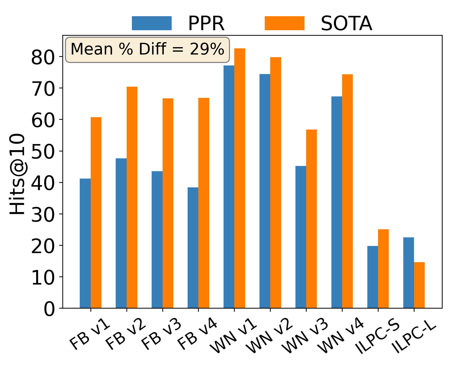
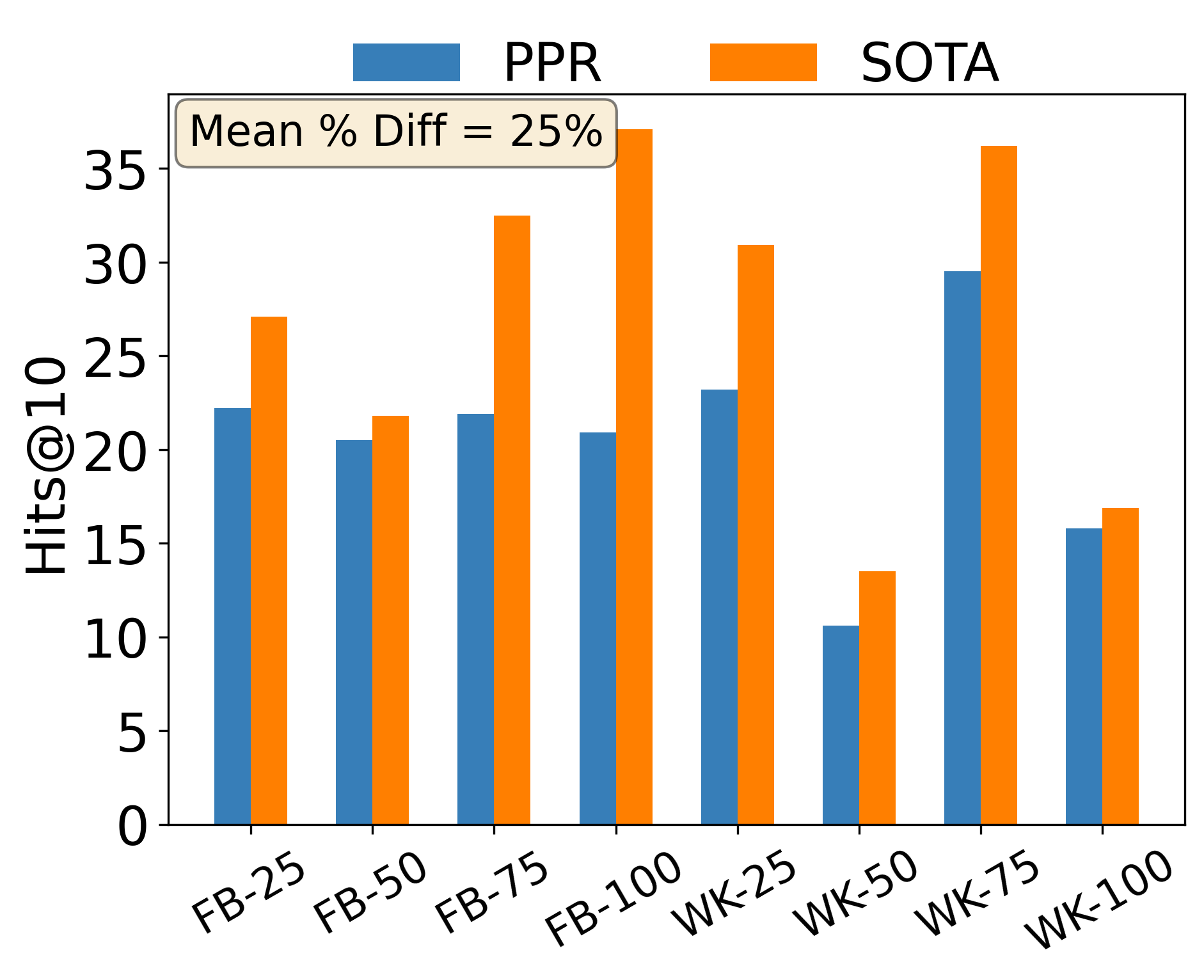
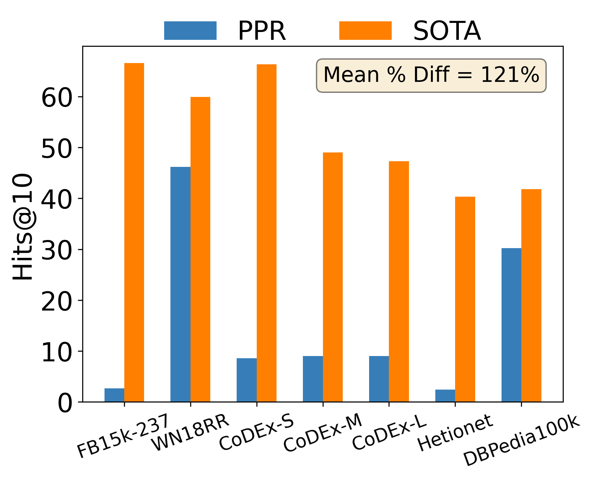
However, we find that on almost all inductive datasets, we can achieve competitive performance by using the Personalized PageRank [12] (PPR) score to perform inference. We note that PPR is a non-learnable heuristic and ignores the relational information in the graph. In Figure 1, we compare the performance of PPR against the supervised SOTA performance on both inductive and transductive datasets. We can see that when performing KGC on inference graphs with either new entities (E) or new entities and relations (E, R), PPR performs only roughly 25% worse than SOTA. However, this is generally not true for transductive datasets, where PPR usually performs poorly. Interestingly, this observation is true for inductive datasets even when the transductive dataset that it is created from has poor PPR performance. For example, while PPR performs very poorly on FB15k-237, it achieves higher performance on it’s inductive derivatives (denoted by “FB”). These findings are problematic as PPR has no basis in literature as a heuristic for KGC, since it completely overlooks the relational aspect of KGs. Therefore, this suggests the potential existence of a shortcut that allows a simple non-learnable method like PPR to achieve high performance on almost all inductive datasets . This also brings into question how successful most methods are in inductive reasoning, as a large portion of their performance may be due to this shortcut.
This finding naturally motivates us to ask – why can PPR perform so well on existing inductive datasets? In Section 3 we discover that the high performance of PPR is due to how the inductive datasets are created from transductive datasets. Specifically, we observe that the current procedure creates graphs where the shortest path distance (SPD) between entities in positive test samples is much lower than the SPD between those in negative samples. This allows for a method like PPR, which gives a higher weight to shorter walks, to distinguish between the positive and negative samples based solely on the distance. To account for this problem, in Section 4 we propose a new strategy for sampling inductive datasets that uses graph partitioning to create the train and inference graphs. This allows us to sample subgraphs that retain the general properties of the original graph. We then demonstrate that this procedure can indeed create inductive datasets that limit the performance ability of PPR. Lastly, we benchmark common inductive KGC methods on our newly constructed datasets. Our key contributions can be summarized as follows:
-
•
We observe that on existing inductive KGC datasets, we can achieve competitive performance when ranking entities using only the Personalized PageRank score.
-
•
Through empirical study, we find that the strong performance of PPR on inductive datasets is due to the current procedure for constructing those datasets, which allows for a shortcut to distinguish between positive and negative samples.
-
•
We propose a new strategy for sampling inductive KGC datasets from their transductive counterparts that uses graph partitioning. We show that our proposed method can substantially mitigate the shortcut. We then benchmark popular inductive KGC method on our newly created datasets. Compared to the older datasets, previous SOTA tend to decrease in performance.
The remaining paper is structured as follows. In Section 2, we provide background on inductive KGC methods, datasets, and PPR. In Section 3, we study in detail when and why PPR can perform well on inductive KGC. We then introduce our new strategy for creating inductive datasets in Section 4 and benchmark popular methods on these newly created datasets in Section 5.
2 Background
Throughout this study we denote a knowledge graph as where is a set of entities (i.e., nodes), the set of relations (i.e., edge types), and the set of edges (i.e., triples) of the form where and are entities and a relation. Lastly, we note that the task of KGC is formulated as the following where given a query , we attempt to predict the correct entity .
Inductive KGC Datasets: In inductive KGC, we are given a training graph and an inference graph . A method is trained on and evaluated on . Most datasets consider the setting that is only disjoint on the entities such that and . This setting is referred to as the (E) setting. Another setting, which we denote as (E, R) further allows to contain relations not in .
All existing inductive datasets are sampled from existing transductive datasets. Furthermore, the majority of inductive datasets [7, 9] are further created via the same procedure introduced by [7]. We give brief overview of this procedure below. Given a transductive dataset, which we denote as , seed entities are randomly chosen from . The 2-hop neighborhood is then extracted around each individual seed entity. To prevent exponential growth, the number of neighbors sampled at any hop is capped at 50 for each individual seed entity. The resulting edges are then combined to create and are subsequently removed from the original graph. The inference graph is then sampled in a similar manner from the resulting graph . We note that the one exception to this procedure are the ILPC datasets, introduced by [10], which instead sample of the nodes from and use them to create . The rest of the nodes are then used to construct . In practice, we find that both sampling methods tend to produce similar graphs.
Inductive KGC Methods: Both NeurlLP [13] and DRUM [14] consider combining the path representations of different length between both entities in a triple. However, since they explicitly consider each path, they are often limited to only considering paths of up to length 2 or 3. Conditional MPNNs [15] are a more efficient alternative to encoding higher-order path information. They work by conditioning the message passing mechanism on the known entity, allowing the implicit aggregation of all paths up to a length (which is equal to the number of GNN layers). The value of is typically . Prominent examples include NBFNet [8] and RED-GNN [11]. More scalable alternatives have been proposed that prune the propagated messages [16, 17, 18]. NodePiece [19] is concerned with parameter efficiency, using an anchor-based approach to learn a more compact set of entity and relation representations. All previous methods assume that a fixed set of relations exist between the train and inference graphs. To account for new relations in inference, InGRAM [9] introduces the concept of a “relation graph”, which inductively encodes the representation of each relation. Note that we omit subgraph methods that have been to shown to prohibitively expensive [7, 20, 21, 22, 23] or those that require the use of external textual information [24].
Personalized PageRank: PageRank [12] computes the probability of finishing a random walk of arbitrary length at some node , when there is equal probability of beginning the walk at any node in the graph. Personalized PageRank (PPR) [12] is a version of PageRank that is “personalized" to some root node , where at each step there is a probability of teleporting to . The set of PPR scores for a root node is given by and can be formulated as the weighted sum of all random walk probabilities between two nodes [25]:
| (1) |
where is the random walk matrix and is a one-hot vector at node . Intuitively, we can see that weight given to a walk decays with the increase in length due to . As such, the PPR score will often be higher for those nodes of shorter distance to . Note that for a KG, we obtain the PPR matrix by first converting the inference graph, , to an undirected graph. We note that this is common practice in KGC [26] whereby inverse relations are added to the graph. We further assume an edge weight of 1 for all edges.
3 Preliminary Study
In this section, we examine the performance on common inductive KGC datasets. We first show that the Personalized PageRank (PPR) can often serve as a good baseline on most datasets. From this observation, we attempt to answer two important questions: (1) When can the PPR scores perform well on KGC? and (2) Why can PPR sometimes perform well for KGC?
3.1 Personalized Pagerank (PPR) is a Strong Baseline for Inductive KGC
We begin by obtaining the PPR matrix of the inference graph for use in evaluation. See Section 2 for more details on how this is done. Given this new graph, for a query , we calculate the PPR score for all possible entities . Using these scores, we can obtain the rank of the true entity for the query and compute the performance in terms of Hits@10.
In Figure 1, we show the performance when using the PPR versus the SOTA performance among supervised methods. We split the datasets by transductive, (E), and (E, R) inductive. We include those datasets most often used in each task, comprising 25 in total. See Appendix B.1 for more details on the datasets chosen. The full set of results can be found in Appendix A.1. We observe that on both types of inductive datasets, the PPR score does reasonably well, performing on average only 25-29% less than SOTA. Also, on some datasets like the WN or ILPC inductive splits, the performance nearly matches or exceeds the supervised performance. On the other hand, for the transductive datasets, the performance disparity is often much larger. Interestingly, PPR still performs well on some transductive datasets, including the popular WN18RR. This tells us that this phenomenon is not unique to inductive datasets. However, this phenomenon is far less common on transductive datasets.
Curiously, for the inductive datasets, their performance using PPR is much higher than their transductive parents. For example, on the inductive datasets derived from FB15k-237, the performance of PPR increases by an average of 1,186%. Furthermore, for those derived from WN18RR, they see an average increase of 43%. This suggests that there is some change in the underlying inductive graphs that are causing the performance of PPR to increase.
3.2 When Does PPR Perform Well and Why?
In the previous section we detailed that PPR score performs well on the inductive setting. Furthermore, the performance of PPR on inductive datasets is much higher than their transductive counterparts of which they’re derived from. This raises the question – why can PPR perform well on some datasets but not others?
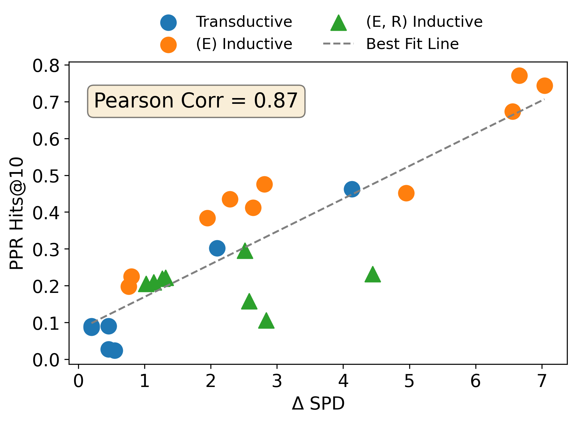
We find that the answer lies in comparing the mean shortest path distance (SPD) between positive and negative samples. For a query , let denote the correct answer and as the set of negative answers for the query. We compute the SPD on the inference graph for both and . This is repeated for each test sample . We then calculate the mean SPD across all positive and negative test samples, which we denote as and , respectively. The different in mean SPD is correspondingly given by . This tells us, on average, how much shorter the distance between entities in positive samples are relative to those in negatives.
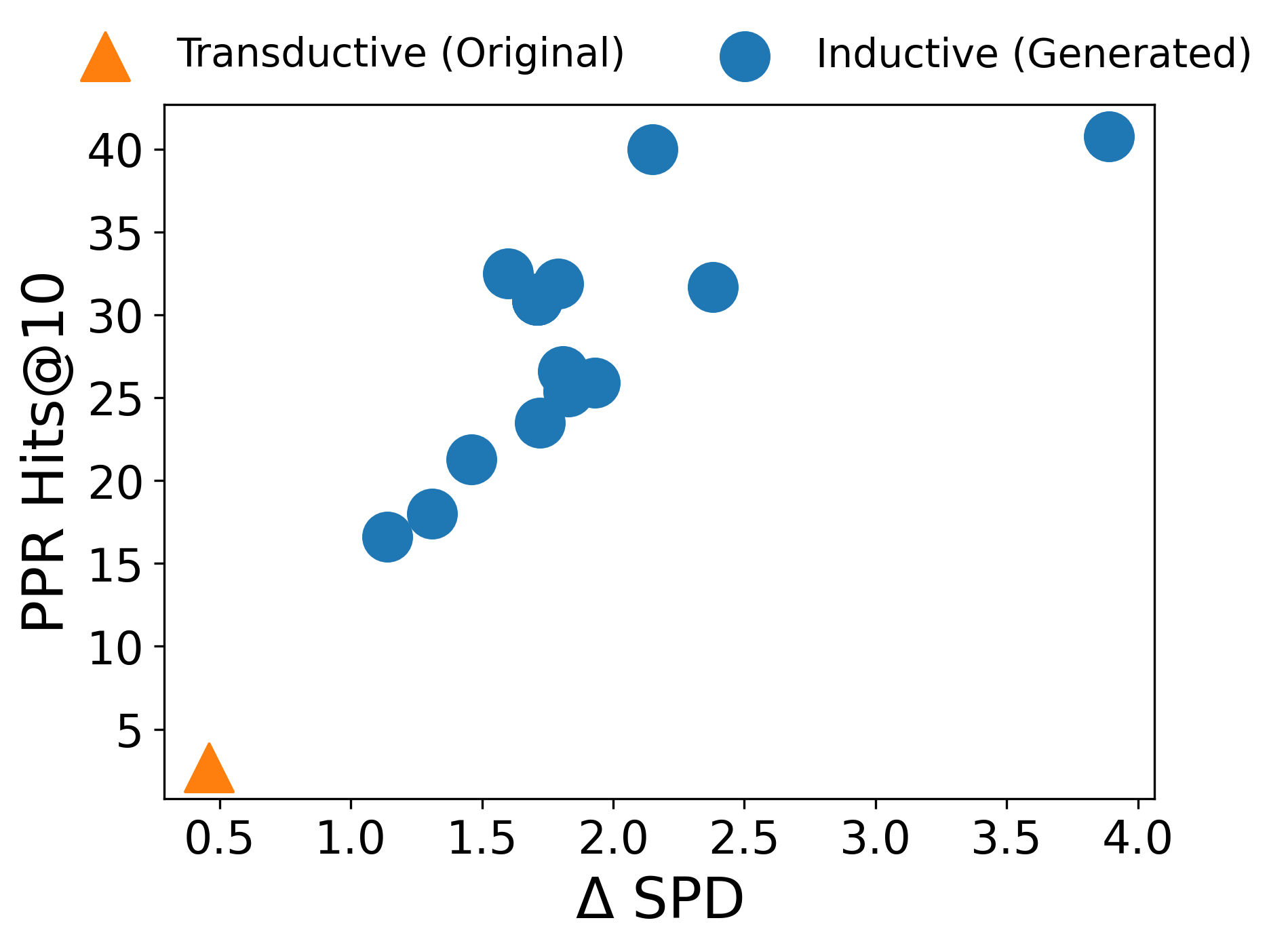
In Figure 2 we show the relationship between and the Hits@10 when using PPR. The results are across 25 different datasets, for both inductive and transductive KGC. Calculating the Pearson correlation, we can observe it is 0.87, which indicates a strong relationship between the two metrics. Therefore, there exists a basic pattern to distinguish positive and negative samples in many KGC datasets. Put simply, the SPD between entities in positive test samples tend to be lower than that in negative samples. The larger the discrepancy between the mean distances, the better PPR can perform. This suggests that the PPR scores can exploit this distance disparity in the datasets to achieve good performance, even while completely ignoring the relational information.
But, why can PPR exploit this pattern? As shown in Eq. (1), the PPR score between two nodes is the weighted sum of random walk probabilities between them. Furthermore, walks of shorter length are weighed more heavily than those of longer length. Therefore, nodes with a shorter distance between them will be able to benefit from these highly-weighted walks, while those of larger distance will not. For example, when , the weight of a walk with is while when it is . As such, the PPR score will invariably favor those node pairs with a lower SPD.
Note that we use PPR as opposed to SPD in our experiments since all-pairs SPD is costly to calculate and the full PPR matrix can be efficiently approximated via [27]. Furthermore, as we show in Section 3.3, even when controlling for the SPD, the PPR score can help differentiate between positive and negative samples.
3.3 Why is This So Common on Inductive Datasets?
In the last section, we covered when PPR can perform well on KGC and why. However, one remaining question is – why is this trend so pervasive on inductive datasets but rarely on their transductive counterparts? For example, on FB15k-237 [28], a transductive dataset, the Hits@10 of PPR is 2.7%. However, across eight different inductive versions of FB15k-237, the mean PPR performance is 32%. We find that this can be explained by the following two observations.
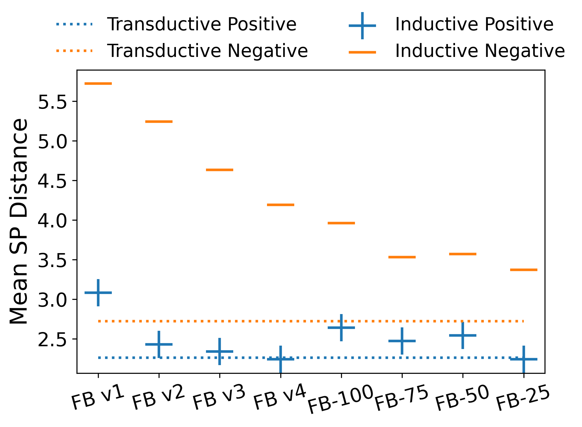
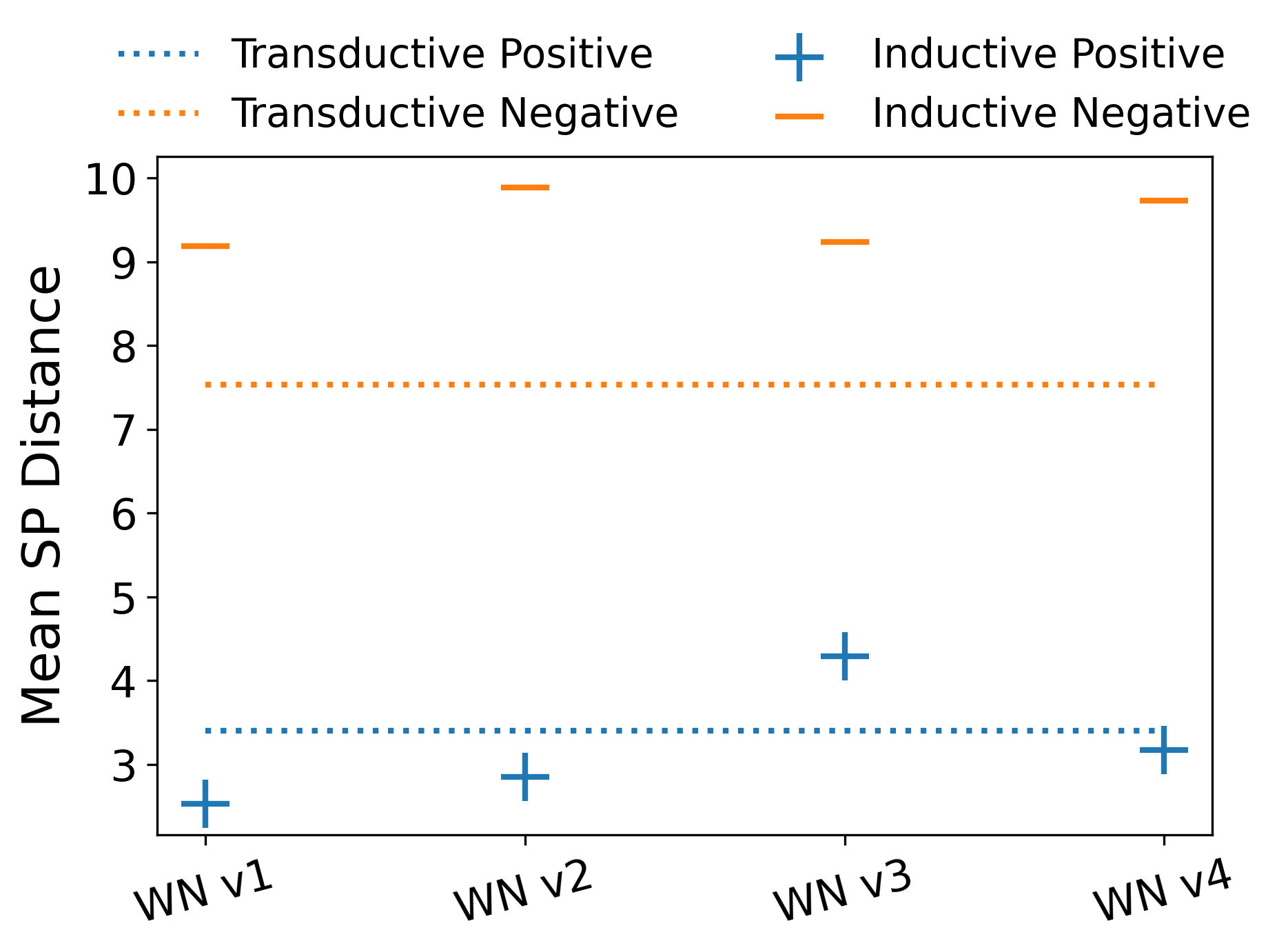
Observation 1: The current procedure for creating inductive datasets increases the and thereby the performance of PPR. As noted earlier, all common inductive datasets are created from existing transductive datasets. See Section 2 for a detailed overview of the construction process. In a nutshell, the training and inference graph are constructed sequentially by sampling a number of subgraphs from a graph. In Figure 3 we show the mean SPD of both positive and negative samples for 12 inductive datasets and their parent transductive dataset. We limit our analysis to those datasets derived from FB15k-237 and WN18RR, as the majority of inductive datasets are derived from them. We observe that for all inductive datasets, while the mean SPD for negative samples sharply rises, the mean SPD for positive samples stay roughly the same. This creates the shortcut described in Section 3.2, where the SPD can easily differentiate between positive and negative samples. Since the gap between the distances is almost always larger than the original transductive dataset, this shortcut becomes more pronounced, thereby leading to a better PPR performance (see Appendix A.1 for detailed results).
But why does the mean SPD drastically change for negative samples but not positive? We find that this is due to the fact that entities in positive samples are more well-connected those those in negatives. In Table 1, we show the % difference in mean PPR score between positive and negative samples when controlling for the SPD on two inductive datasets.
| SPD Range | WN18RR v4 | FB15k-237 v4 |
| +17% | +5% | |
| +29% | +200% | |
| +82% | +328% | |
| +2837% | +44% |
We can see that the PPR score is much greater for positive samples, even for higher values of SPD. Therefore, the SPD of positive samples are better able to “withstand" changes in the underlying graph better than negatives, as they typically contain additional shorter walks between samples. However, negatives samples are typically much less well-connected, so they are more affected by removing a portion of edges from the original graph.
Observation 2: Constructing a good inductive dataset is difficult. In Section 2 we discuss the general algorithm used to create inductive datasets. Multiple parameters exist that guide the construction process. It is tempting to think that by simply trying different combinations, one can happen upon a split that doesn’t suffer from high PPR performance. However, in practice, we find that this is difficult, as there are multiple factors to contend with.
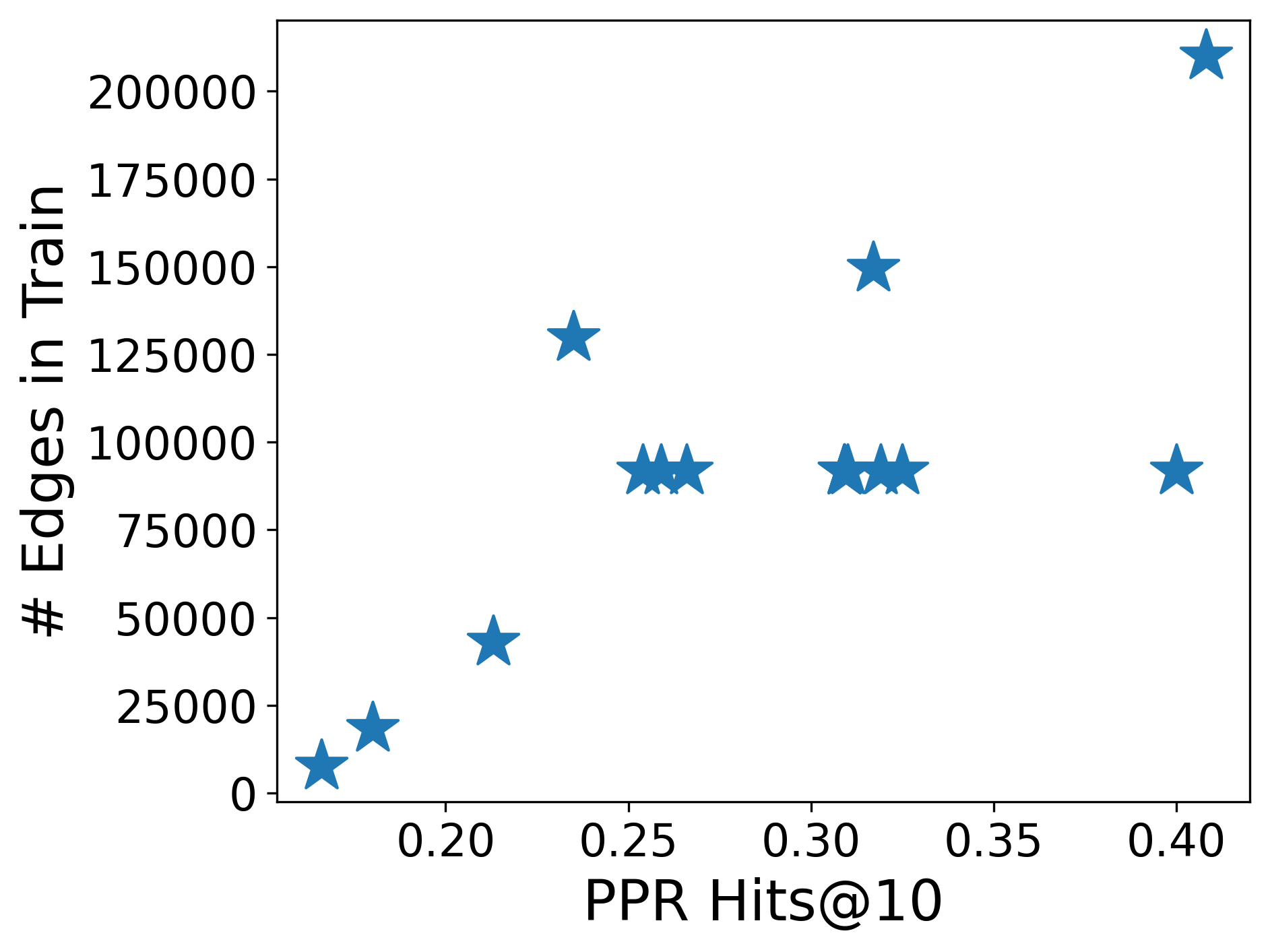
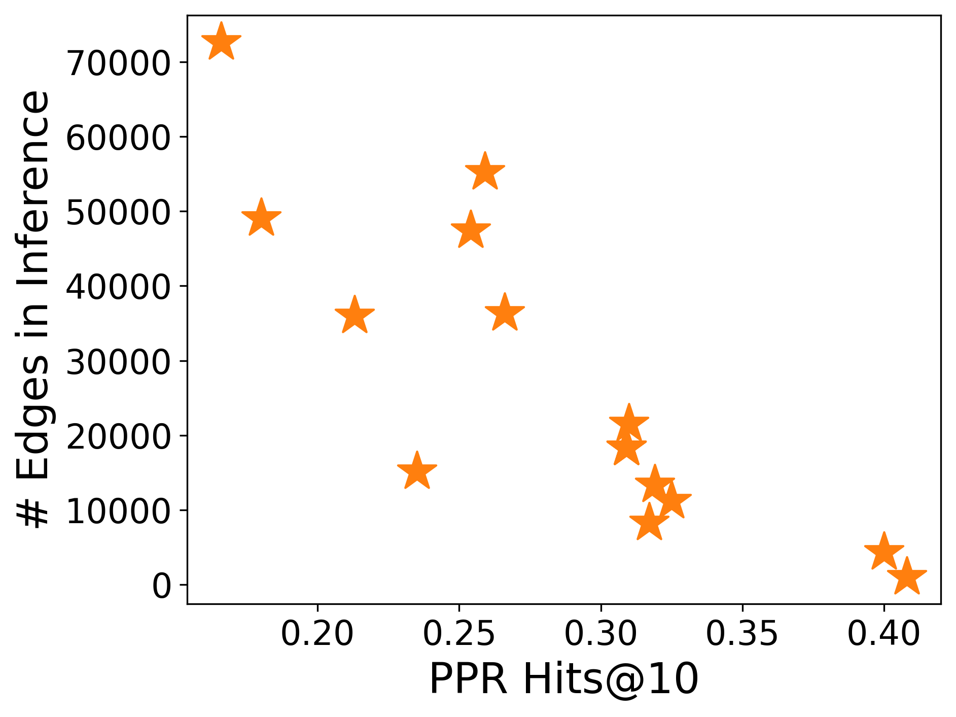
We demonstrate this by attempting to generate inductive datasets from FB15k-237. We generate a number of different inductive datasets by modifying the (a) # of seed entities for train and inference and (b) the maximum neighborhood size for train and inference. For different combination of values, we generate three different datasets using different random seeds. For each of the generated datasets, we calculate the size of both the train and inference graphs, the , and the PPR performance. These values are then averaged across seeds. A more detailed discussion is given in Appendix C. In Figure 4(a) we plot the vs. the PPR performance. Despite searching across a wide variety of parameters, both and the PPR performance remain much higher for the inductive datasets compared to the transductive dataset. Furthermore, we show the relationship between the size of the train and inference graphs and the PPR performance in Figures 4(b) and 4(c). We observe that when the performance of PPR is at its lowest, the size of the train graph is noticeably small. However, fixing this problem, results in a sharp increase in the performance of PPR. Furthermore, there is an inverse relationship between the size of the train and inference graph, making it hard to find a “sweet spot” where the PPR performance is low and both graphs aren’t too small.
The studies in this section show that the current strategy for constructing inductive datasets from existing transductive datasets is liable to introduce a well-performing shortcut into the existing graph. Currently, it almost always leads to a sharp increase in the PPR performance. Furthermore, attempting to limit the severity of this issue is very difficult while also generating train and inference graphs of reasonable sizes. This suggests that a new strategy is needed for sampling graphs for inductive KGC from transductive datasets.
4 Constructing Inductive Datasets through Graph Partitioning
In the previous section, we showed that the PPR score can achieve strong performance on most inductive KGC datasets. Furthermore, we demonstrate that this is due to how inductive datasets are sampled from existing transductive datasets. This sampling strategy engenders a shift in the underlying properties of the graph that allows for PPR to perform well. This naturally causes us to ask – How can we mitigate this problem when constructing newer inductive datasets? In the next subsection, we introduce our strategy which utilizes graph partitioning to alleviate this problem.
4.1 Partition-Based Dataset Sampling
We’ve previously covered in Section 3 that the existing procedure for creating inductive datasets leads to suboptimal subgraphs. This is because the resulting subgraphs tend to have much different properties than the original graph, such as the distance distribution, which can potentially lead to shortcuts when performing KGC.
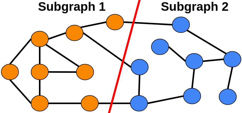
We note that the task of constructing inductive datasets from an existing graph can be framed as a graph partitioning problem. Formally, we want to sample two non-overlapping partitions from the graph such that . Given the analysis in Section 3.2, we hope to sample subgraphs such that ). But, how do we find subgraphs that satisfy this property? Intuitively, we want to sample each subgraph so that it’s removal has little effect on the initial graph’s structure. We give an example in Figure 5 where we sample two subgraphs from an existing graph. As we can see, even though the graph is partitioned, the relationship between entities in the same partition remain roughly the same before and after the partition. This is because there already exists little relationship between the two partitions in the original graph.
| Task | Dataset | PPR Hits@10 | |||||
| Trans. | Ind. New | Ind. Old | Trans. | Ind. New | Ind. Old | ||
| (E) | WN18RR | 46.2 | 45.1 | 66.0 | 4.1 | 3.2 | 6.3 |
| CoDEx-M | 9.0 | 11.2 | 21.1 | 0.2 | 0.24 | 0.78 | |
| HetioNet | 2.7 | 2.4 | NA | 0.55 | 0.29 | NA | |
| (E, R) | FB15k-237 | 2.7 | 10.8 | 21.4 | 0.46 | 0.48 | 2.42 |
| CoDEx-M | 9.0 | 13.2 | NA | 0.20 | 0.42 | NA | |
Multiple popular approaches [29, 30] exist that attempt to divide the graph into optimal partitions. The guiding principle in these approaches is that the partitions should be internally dense but only sparsely connected to one another. Because of this, the entities in different partitions should only be weakly connected and have little impact on one another. Therefore, the relationship between entities in the same partition are minimally affected by outside entities or edges. As such, removing this partition from the graph should then have little effect on the entities in that partition. Also, since the partitions are created at the same time, we avoid sampling the inference graph after the training, which can be suboptimal.
In practice, we consider using Spectral Clustering [29] or the Louvain method [30], as dependent on the dataset. Once the original graph is partitioned into partitions, we sample of those to be used. The partitions are chosen such that they display similar properties to the original graph (see Section 4.2 for more). Of the partitions, one is chosen as the training graph while the other are designated as separate inference graphs. This is an important advantage of using partitioning to sample the graphs, as it allows us to avoid having to sample multiple different train and inference pairs as in [7, 9], thereby allowing for more efficient benchmarking. Lastly, we note that when sampling graphs for the (E) inductive task, we further remove new relations from the inference graph. In practice, we find that we can easily find partitions where this amounts to little or no change in the inference graph. See Section B.2 for more details on the dataset creation process.
4.2 Analysis of New Datasets
In this section we analyze the new inductive datasets created following the partition-based procedure outlined in Section 4.1. We create (E) inductive datasets, from WN18RR [26], CoDEx-M [31], and HetioNet [32]. For the (E, R) datasets, we use CoDEx-M [31] and FB15k-237 [28]. Each dataset has two separate inference graph except for CoDEx-M on the (E) task which has one. Note that some datasets are only suitable for one task or another. For example, WN18RR and HetioNet have very few relations, making it nearly impossible to sample two partitions with significantly different relations for the (E, R) task. On the other hand, FB15k-237 contains too many relations to sample multiple graphs for the (E) task without removing many edges from either the train or inference graph.
In Table 2 we show the PPR Hits@10 and for the inductive datasets and their original transductive dataset. We note that when multiple inference graphs exist, we take the mean across each inference graph. When possible, we also include a comparison against those inductive datasets that already exist. For example, for WN18RR in the (E) task, 4 datasets exist from [7]. As compared to the old inductive datasets, the PPR performance for the new inductive datasets is much lower. On average, the performance of PPR is 78% lower for the new inductive datasets. Furthermore, the PPR performance of the new inductive datasets is very similar to the performance on the original transductive dataset. A similar trend can be found when comparing the . This analysis shows that newer sampling procedure can indeed sample inductive datasets that are much more similar to the original transductive graph. Furthermore, it greatly helps mitigate the PPR shortcut.
5 Experiments
5.1 Experimental Settings
Datasets: We use the new datasets created in Section 4.1. For the (E) setting, this includes WN18RR, HetioNet, and CoDEx-M. For the (E, R) setting, it is FB15k-237 and CoDEx-M. We sample 2 inference graphs for each dataset, except for CoDEx-M on the (E) setting where we could only find 1 suitable graph for inference. For each inference graph, 10% of edges are randomly removed for testing. For validation 10% of edges are removed from the training graph. It is necessary that the validation samples are extracted from the train graph as the inference graphs must remain unobserved during training. The statistics for each dataset can be found in Appendix B.2.
Baseline Methods: We consider prominent KGC methods including NBFNet [8], RED-GNN [11], NodePiece [19], and InGram [9]. We also consider the recent foundation model ULTRA [33].
Hyperparameters: The exact hyperparameters and their ranges differ by method due to difference in implementations. For each method, we tried to follow the recommended ranges used by the authors. For InGram [9] we tuned the learning rate in and the number of entity layers in . For NodePiece [19] we tuned the learning rate from and the loss margin from . For RED-GNN [11], we tuned the learning rate from and the dropout from . In their experiments, NBFNet [8] uses the same hyperparameters across all datasets. We therefore do the same.
The full set of experimental settings can be found in Appendix D.
5.2 Results
| Models | CoDEx-M | WN18RR | HetioNet | ||
| Inference 1 | Inference 1 | Inference 2 | Inference 1 | Inference 2 | |
| PPR | 11.2 | 66.2 | 24 | 3.2 | 2.2 |
| NodePiece | 6.8 ± 0.8 | 29.6 ± 0.8 | 4.8 ± 0.6 | 10.2 ± 0.9 | 15.4 ± 0.9 |
| InGram | 20.1 ± 3.5 | 38.0 ± 2.4 | 8.0 ± 2.9 | 21.9 ± 1.1 | 22.3 ± 2.8 |
| RED-GNN | 35.6 ± 2.3 | 72.9 ± 0.4 | 27.7 ± 0.3 | 68.3 ± 3.0 | 85.1 ± 2.7 |
| NBFNet | 43.6 ± 0.2 | 75.5 ± 0.2 | 29.4 ± 2.5 | 72.8 ± 3.8 | 77.2 ± 0.4 |
Models FB15k-237 CoDEx-M Inference 1 (27%) Inference 2 (63%) Inference 1 (10%) Inference 2 (57%) MRR Hits@10 MRR Hits@10 MRR Hits@10 MRR Hits@10 PPR 3.8 9.1 4.7 12.4 3.3 10.9 7.1 15.4 NodePiece 1.4 ± 0.1 3.0 ± 0.6 2.6 ± 0.2 4.7 ± 0.5 1.5 ± 0.2 3.1 ± 0.6 1.6 ± 0.4 2.5 ± 1.0 InGram 11.2 ± 1.9 23.8 ± 3.0 9.2 ± 0.9 20.2 ± 2.0 10.3 ± 1.2 20.4 ± 3.3 7.2 ± 4.2 15.9 ± 10.0 RED-GNN 11.8 ± 2.8 21.6 ± 5.8 19.8 ± 2.2 33.3 ± 4.2 16.8 ± 1.6 29.2 ± 2.9 14.7 ± 5.3 26.5 ± 10.4 NBFNet 15.8 ± 0.9 27.5 ± 1.8 15.9 ± 0.2 26.2 ± 0.3 27.9 ± 8.8 47.7 ± 11.8 8.5 ± 4.8 17.6 ± 10.0
Main Results: The main results for supervised methods can be found in Tables 3 and 4. We observe that on nearly every dataset, NBFNet and RED-GNN are the two best models. This indicates that conditional MPNNs [15], the class of model in which both belong to, are necessary for strong performance in inductive KGC. Interestingly, we observe that InGram struggles in the (E, R) setting. This is even true when the % of new relations is high. This run counters to the results on older inductive datasets [9] where InGram excelled over NBFNet and RED-GNN. Lastly, outside of NodePiece, each method is usually able to significantly outperform PPR.
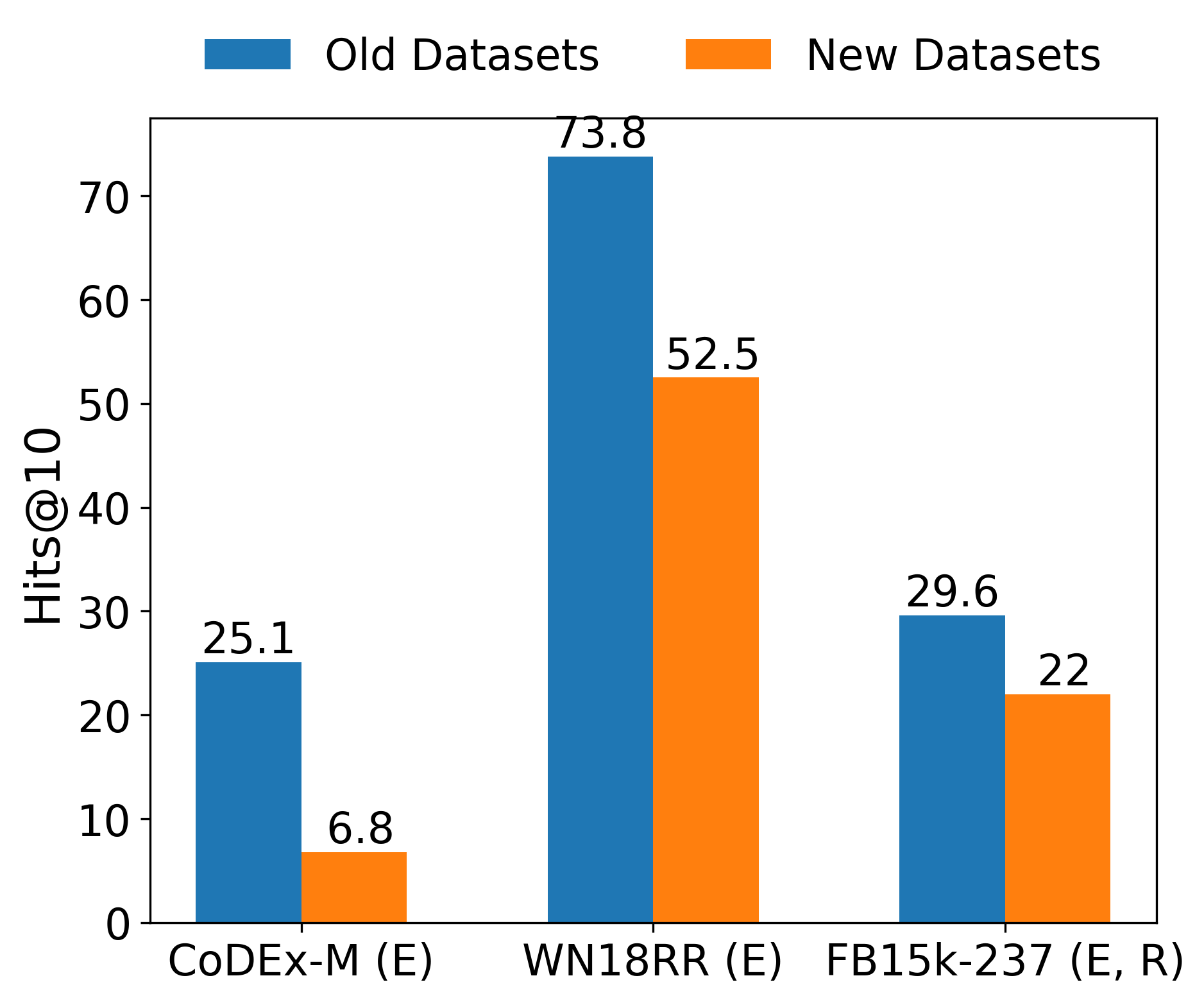
Performance Comparison on New and Old Inductive Datasets: We compare the change in performance from the previous inductive datasets to our new datasets. Note that we only compare when there is a corresponding dataset sampled from the same transductive dataset and for the same task. For the (E) task, this includes CoDEx-M (ILPC-S [10]) and WN18RR (v1-v4 [7]). For the (E, R) task it is only FB15k-237 (25-100 [9]). For each, we compare the performance of the SOTA on the older dataset to their corresponding performance on the new datasets. This is NBFNet [8] for WN18RR and FB15k-237 and NodePiece [19] for CoDEx-M. We only compare the performance of the old SOTA as not all methods were tested on the older datasets or guranteed to be well-tuned. The results are shown in Figure 6(a). We find that performance on each of the new datasets drops significantly. This suggests that removing the shortcut has a large negative effect on the performance.
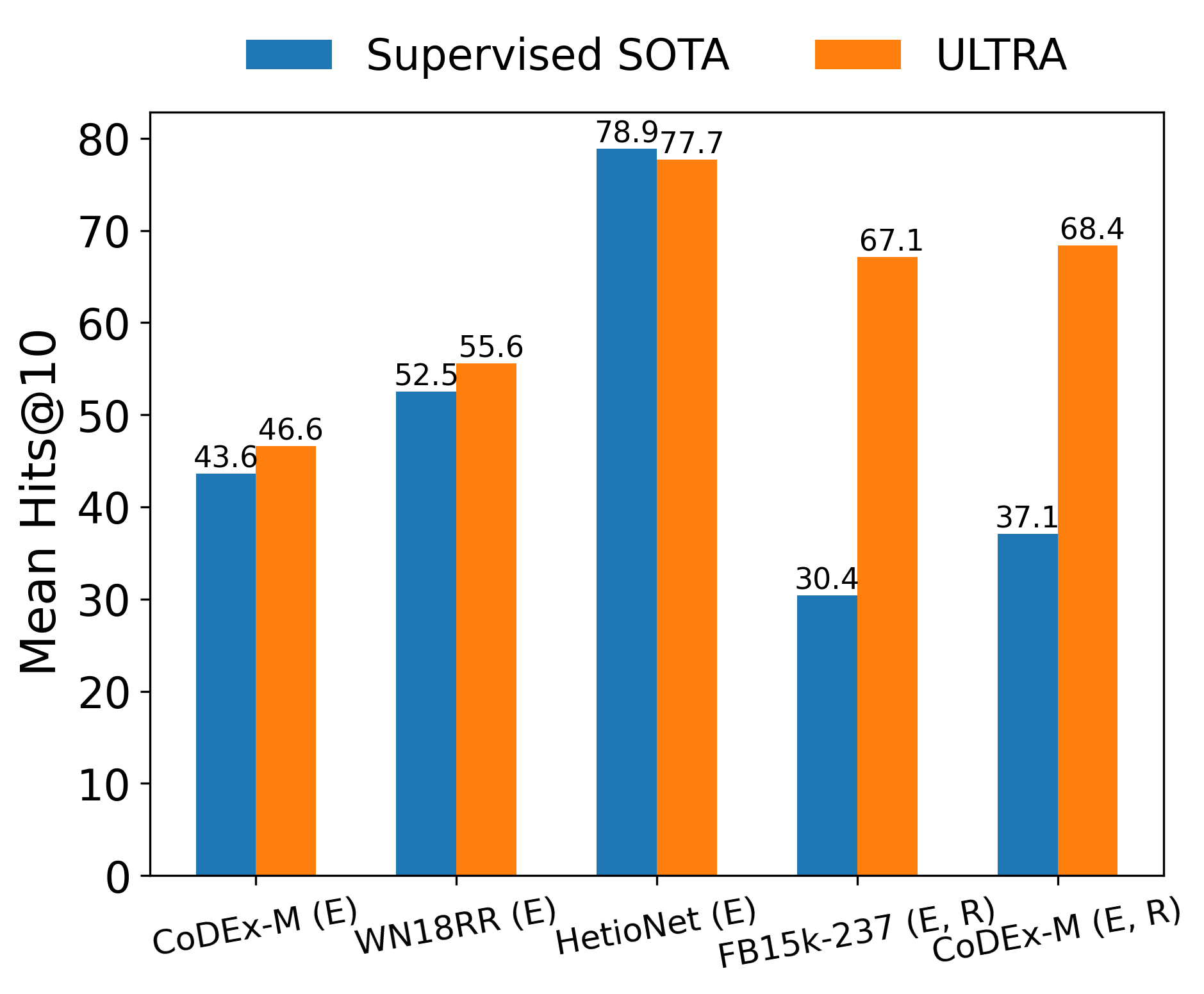
Performance of ULTRA [33]: We further compare against ULTRA, a recent foundation model designed for fully inductive KGC. We evaluate ULTRA under the 0-shot setting. See Appendix E for more details on the version of ULTRA used. The results are in Figure 6(b) where for each dataset, we average the results across the different inference graphs (full results in Appendix A.2). On the (E) task, ULTRA is comparable to the supervised SOTA. However, on the (E, R) task, ULTRA significantly outperforms other methods. This suggests that ULTRA contains a much greater ability to generalize to unseen relations than existing supervised methods.
6 Conclusion
In this paper we study the problem of constructing datasets for inductive knowledge graph completion. Upon examination, we find that we can achieve competitive performance on most inductive datasets through the use of Personalized PageRank [12], which ignores the relational structure of the graph. Through our study, we uncover that this shortcut is due to how inductive datasets are created. To remedy this problem, we propose a new dataset construction process based on graph partitioning that helps mitigate the impact of the studied shortcut. We then construct new benchmark datasets using this new procedure and benchmark various methods.
References
- [1] Xiangxiang Zeng, Xinqi Tu, Yuansheng Liu, Xiangzheng Fu, and Yansen Su. Toward better drug discovery with knowledge graph. Current opinion in structural biology, 72:114–126, 2022.
- [2] Payal Chandak, Kexin Huang, and Marinka Zitnik. Building a knowledge graph to enable precision medicine. Scientific Data, 10(1):67, 2023.
- [3] Xiang Wang, Tinglin Huang, Dingxian Wang, Yancheng Yuan, Zhenguang Liu, Xiangnan He, and Tat-Seng Chua. Learning intents behind interactions with knowledge graph for recommendation. In Proceedings of the web conference 2021, pages 878–887, 2021.
- [4] Antoine Bordes, Nicolas Usunier, Alberto Garcia-Duran, Jason Weston, and Oksana Yakhnenko. Translating embeddings for modeling multi-relational data. Advances in neural information processing systems, 26, 2013.
- [5] Théo Trouillon, Johannes Welbl, Sebastian Riedel, Éric Gaussier, and Guillaume Bouchard. Complex embeddings for simple link prediction. In International conference on machine learning, pages 2071–2080. PMLR, 2016.
- [6] Michael Schlichtkrull, Thomas N Kipf, Peter Bloem, Rianne Van Den Berg, Ivan Titov, and Max Welling. Modeling relational data with graph convolutional networks. In European semantic web conference, pages 593–607. Springer, 2018.
- [7] Komal Teru, Etienne Denis, and Will Hamilton. Inductive relation prediction by subgraph reasoning. In International Conference on Machine Learning, pages 9448–9457. PMLR, 2020.
- [8] Zhaocheng Zhu, Zuobai Zhang, Louis-Pascal Xhonneux, and Jian Tang. Neural bellman-ford networks: A general graph neural network framework for link prediction. Advances in Neural Information Processing Systems, 34:29476–29490, 2021.
- [9] Jaejun Lee, Chanyoung Chung, and Joyce Jiyoung Whang. Ingram: Inductive knowledge graph embedding via relation graphs. In International Conference on Machine Learning, pages 18796–18809. PMLR, 2023.
- [10] Mikhail Galkin, Max Berrendorf, and Charles Tapley Hoyt. An open challenge for inductive link prediction on knowledge graphs. arXiv preprint arXiv:2203.01520, 2022.
- [11] Yongqi Zhang and Quanming Yao. Knowledge graph reasoning with relational digraph. In Proceedings of the ACM Web Conference 2022, pages 912–924, 2022.
- [12] Lawrence Page, Sergey Brin, Rajeev Motwani, and Terry Winograd. The pagerank citation ranking: Bringing order to the web. Technical report, Stanford InfoLab, 1999.
- [13] Fan Yang, Zhilin Yang, and William W Cohen. Differentiable learning of logical rules for knowledge base reasoning. Advances in neural information processing systems, 30, 2017.
- [14] Ali Sadeghian, Mohammadreza Armandpour, Patrick Ding, and Daisy Zhe Wang. Drum: End-to-end differentiable rule mining on knowledge graphs. Advances in Neural Information Processing Systems, 32, 2019.
- [15] Xingyue Huang, Miguel Romero, Ismail Ceylan, and Pablo Barceló. A theory of link prediction via relational weisfeiler-leman on knowledge graphs. Advances in Neural Information Processing Systems, 36, 2024.
- [16] Zhaocheng Zhu, Xinyu Yuan, Louis-Pascal Xhonneux, Ming Zhang, Maxime Gazeau, and Jian Tang. Learning to efficiently propagate for reasoning on knowledge graphs. arXiv preprint arXiv:2206.04798, 2022.
- [17] Yongqi Zhang, Zhanke Zhou, Quanming Yao, Xiaowen Chu, and Bo Han. Adaprop: Learning adaptive propagation for graph neural network based knowledge graph reasoning. In KDD, 2023.
- [18] Harry Shomer, Yao Ma, Juanhui Li, Bo Wu, Charu Aggarwal, and Jiliang Tang. Distance-based propagation for efficient knowledge graph reasoning. In Proceedings of the 2023 Conference on Empirical Methods in Natural Language Processing, pages 14692–14707, 2023.
- [19] Mikhail Galkin, Etienne Denis, Jiapeng Wu, and William L Hamilton. Nodepiece: Compositional and parameter-efficient representations of large knowledge graphs. In International Conference on Learning Representations, 2021.
- [20] Shuwen Liu, Bernardo Grau, Ian Horrocks, and Egor Kostylev. Indigo: Gnn-based inductive knowledge graph completion using pair-wise encoding. Advances in Neural Information Processing Systems, 34:2034–2045, 2021.
- [21] Sijie Mai, Shuangjia Zheng, Yuedong Yang, and Haifeng Hu. Communicative message passing for inductive relation reasoning. In Proceedings of the AAAI Conference on Artificial Intelligence, volume 35, pages 4294–4302, 2021.
- [22] Xiaohan Xu, Peng Zhang, Yongquan He, Chengpeng Chao, and Chaoyang Yan. Subgraph neighboring relations infomax for inductive link prediction on knowledge graphs. arXiv preprint arXiv:2208.00850, 2022.
- [23] Yuxia Geng, Jiaoyan Chen, Jeff Z Pan, Mingyang Chen, Song Jiang, Wen Zhang, and Huajun Chen. Relational message passing for fully inductive knowledge graph completion. In 2023 IEEE 39th International Conference on Data Engineering (ICDE), pages 1221–1233. IEEE, 2023.
- [24] Genet Asefa Gesese, Harald Sack, and Mehwish Alam. Raild: Towards leveraging relation features for inductive link prediction in knowledge graphs. In Proceedings of the 11th International Joint Conference on Knowledge Graphs, pages 82–90, 2022.
- [25] Fan Chung. The heat kernel as the pagerank of a graph. Proceedings of the National Academy of Sciences, 104(50):19735–19740, 2007.
- [26] Tim Dettmers, Pasquale Minervini, Pontus Stenetorp, and Sebastian Riedel. Convolutional 2d knowledge graph embeddings. In Proceedings of the AAAI conference on artificial intelligence, volume 32, 2018.
- [27] Reid Andersen, Fan Chung, and Kevin Lang. Local graph partitioning using pagerank vectors. In 2006 47th Annual IEEE Symposium on Foundations of Computer Science (FOCS’06), pages 475–486. IEEE, 2006.
- [28] Kristina Toutanova and Danqi Chen. Observed versus latent features for knowledge base and text inference. In Proceedings of the 3rd workshop on continuous vector space models and their compositionality, pages 57–66, 2015.
- [29] Jianbo Shi and Jitendra Malik. Normalized cuts and image segmentation. IEEE Transactions on pattern analysis and machine intelligence, 22(8):888–905, 2000.
- [30] Vincent D Blondel, Jean-Loup Guillaume, Renaud Lambiotte, and Etienne Lefebvre. Fast unfolding of communities in large networks. Journal of statistical mechanics: theory and experiment, 2008(10):P10008, 2008.
- [31] Tara Safavi and Danai Koutra. Codex: A comprehensive knowledge graph completion benchmark. In Proceedings of the 2020 Conference on Empirical Methods in Natural Language Processing (EMNLP), pages 8328–8350, 2020.
- [32] Daniel Scott Himmelstein, Antoine Lizee, Christine Hessler, Leo Brueggeman, Sabrina L Chen, Dexter Hadley, Ari Green, Pouya Khankhanian, and Sergio E Baranzini. Systematic integration of biomedical knowledge prioritizes drugs for repurposing. Elife, 6:e26726, 2017.
- [33] Mikhail Galkin, Xinyu Yuan, Hesham Mostafa, Jian Tang, and Zhaocheng Zhu. Towards foundation models for knowledge graph reasoning. In The Twelfth International Conference on Learning Representations, 2023.
- [34] Yihong Chen, Pasquale Minervini, Sebastian Riedel, and Pontus Stenetorp. Relation prediction as an auxiliary training objective for improving multi-relational graph representations. In 3rd Conference on Automated Knowledge Base Construction, 2021.
- [35] Zhiqing Sun, Zhi-Hong Deng, Jian-Yun Nie, and Jian Tang. Rotate: Knowledge graph embedding by relational rotation in complex space. In International Conference on Learning Representations, 2019.
- [36] Boyang Ding, Quan Wang, Bin Wang, and Li Guo. Improving knowledge graph embedding using simple constraints. In Proceedings of the 56th Annual Meeting of the Association for Computational Linguistics (Volume 1: Long Papers), pages 110–121, 2018.
- [37] Farzaneh Mahdisoltani, Joanna Biega, and Fabian M Suchanek. Yago3: A knowledge base from multilingual wikipedias. In CIDR, 2013.
- [38] Farahnaz Akrami, Mohammed Samiul Saeef, Qingheng Zhang, Wei Hu, and Chengkai Li. Realistic re-evaluation of knowledge graph completion methods: An experimental study. In Proceedings of the 2020 ACM SIGMOD International Conference on Management of Data, pages 1995–2010, 2020.
- [39] Adam Paszke, Sam Gross, Francisco Massa, Adam Lerer, James Bradbury, Gregory Chanan, Trevor Killeen, Zeming Lin, Natalia Gimelshein, Luca Antiga, Alban Desmaison, Andreas Kopf, Edward Yang, Zachary DeVito, Martin Raison, Alykhan Tejani, Sasank Chilamkurthy, Benoit Steiner, Lu Fang, Junjie Bai, and Soumith Chintala. Pytorch: An imperative style, high-performance deep learning library. In H. Wallach, H. Larochelle, A. Beygelzimer, F. d'Alché-Buc, E. Fox, and R. Garnett, editors, Advances in Neural Information Processing Systems 32, pages 8024–8035. Curran Associates, Inc., 2019.
- [40] Matthias Fey and Jan E. Lenssen. Fast graph representation learning with PyTorch Geometric. In ICLR Workshop on Representation Learning on Graphs and Manifolds, 2019.
- [41] Wenhan Xiong, Thien Hoang, and William Yang Wang. Deeppath: A reinforcement learning method for knowledge graph reasoning. In Proceedings of the 2017 Conference on Empirical Methods in Natural Language Processing, pages 564–573, 2017.
Appendix A Additional Results
A.1 Supervised SOTA vs. PPR Performance
In this section we show the performance in terms of Hits@10 for the SOTA supervised method vs. the Personalized PageRank (PPR) score. We further include the % difference in performance and which method is considered SOTA. These are shown in Tables 5, 6, and 7 for the (E), (E, R), and transductive datasets, respectively. For an overview of SOTA performance on additional KG datasets, please see [33].
| Dataset | Supervised SOTA | PPR | % Difference | SOTA Method |
| WN v1 | 82.6 | 77.1 | 7% | NBFNet [8] |
| WN v2 | 79.8 | 74.4 | 12% | NBFNet [8] |
| WN v3 | 56.8 | 45.2 | 26% | NBFNet [8] |
| WN v4 | 74.3 | 67.3 | 10% | A*Net [16] |
| FB v1 | 60.7 | 41.2 | 47% | NBFNet [8] |
| FB v2 | 70.4 | 47.6 | 48% | NBFNet [18] |
| FB v3 | 66.7 | 43.5 | 53% | NBFNet [8] |
| FB v4 | 66.8 | 38.4 | 74% | NBFNet [8] |
| ILPC-S | 25.1 | 19.8 | 27% | NodePiece [19] |
| ILPC-L | 14.6 | 22.5 | -35% | NodePiece [19] |
| Dataset | Supervised SOTA | PPR | % Difference | SOTA Method |
| FB-100 | 37.1 | 22.2 | 67% | InGram [9] |
| FB-75 | 32.5 | 21.9 | 48% | InGram [9] |
| FB-50 | 21.8 | 20.5 | 6% | InGram [9] |
| FB-25 | 27.1 | 20.9 | 30% | InGram [9] |
| WK-100 | 16.9 | 15.8 | 7% | InGram [9] |
| WK-75 | 36.2 | 29.5 | 23% | InGram [9] |
| WK-50 | 13.5 | 10.6 | 27% | InGram [9] |
| WK-25 | 30.9 | 23.2 | 33% | InGram [9] |
| Dataset | Supervised SOTA | PPR | % Difference | SOTA Method |
| FB15k-237 | 66.6 | 2.7 | 2367% | NBF+TAGNet [18] |
| WN18RR | 59.9 | 46.2 | 30% | NBF+TAGNet [18] |
| CoDEx-M | 49.0 | 9.0 | 444% | ComplEx RP [34] |
| CoDEx-S | 66.3 | 8.6 | 671% | ComplEx RP [34] |
| CoDEx-L | 47.3 | 9.0 | 426% | ComplEx RP [34] |
| Hetionet | 40.3 | 2.4 | 1579% | RotatE [35] |
| DBPedia100k | 41.8 | 30.2 | 38% | ComplEx-NNE+AER [36] |
A.2 Performance of ULTRA
We include the full results of ULTRA [33] on each dataset and inference graph. The result on the (E) datasets are in Table 8 while those for the (E, R) datasets are in Table 9.
| Metric | CoDEx-M | WN18RR | HetioNet | ||
| Inference 1 | Inference 1 | Inference 2 | Inference 1 | Inference 2 | |
| MRR | 30.2 | 64.7 | 21.4 | 57.9 | 72.7 |
| Hits@10 | 46.6 | 72.7 | 38.5 | 69.1 | 86.3 |
| Metric | FB15k-237 | CoDEx-M | ||
| Inference 1 | Inference 2 | Inference 1 | Inference 2 | |
| MRR | 45.7 | 38 | 30.4 | 73.7 |
| Hits@10 | 69.6 | 64.5 | 45.7 | 91.3 |
Appendix B Datasets
B.1 Existing Datasets
We detail the statistics of all existing transductive and inductive datasets in Tables 10, 11, and 12, respectively. We further include the licenses for each in Table 13. Note that we omit YAGO3-10 [37] as [38] show that the dataset is dominated by two duplicate relations, making most triples trivial to classify. Also, we omit NELL-995 and any inductive datasets derived from it due to findings by [31] that show that most triples in the dataset are either too generic or meaningless.
| Dataset | #Entities | #Relations | #Train | #Validation | #Test |
| FB15k-237 [28] | 14,541 | 237 | 272,115 | 17,535 | 20,466 |
| WN18RR [26] | 40,943 | 11 | 86,835 | 3,034 | 3,134 |
| CoDEx-S [31] | 2,034 | 42 | 32,888 | 1,827 | 1,828 |
| CoDEx-M [31] | 17,050 | 51 | 185,584 | 10,310 | 10,311 |
| CoDEx-L [31] | 77,951 | 69 | 551,193 | 30,622 | 30,622 |
| HetioNet [32] | 45,158 | 24 | 2,025,177 | 112,510 | 112,510 |
| DBpedia100k [36] | 99,604 | 470 | 597,572 | 50,000 | 50,000 |
| Dataset | #Relations | Train Graph | Validation Graph | Test Graph | |||||
| #Entities | #Triples | #Entities | #Triples | #Valid | #Entities | #Triples | #Test | ||
| FB15k-237 v1 [7] | 180 | 1,594 | 4,245 | 1,594 | 4,245 | 489 | 1,093 | 1,993 | 205 |
| FB15k-237 v2 [7] | 200 | 2,608 | 9,739 | 2,608 | 9,739 | 1,166 | 1,660 | 4,145 | 478 |
| FB15k-237 v3 [7] | 215 | 3,668 | 17,986 | 3,668 | 17,986 | 2,194 | 2,501 | 7,406 | 865 |
| FB15k-237 v4 [7] | 219 | 4,707 | 27,203 | 4,707 | 27,203 | 3,352 | 3,051 | 11,714 | 1,424 |
| WN18RR v1 [7] | 9 | 2,746 | 5,410 | 2,746 | 5,410 | 630 | 922 | 1,618 | 188 |
| WN18RR v2 [7] | 10 | 6,954 | 15,262 | 6,954 | 15,262 | 1,838 | 2,757 | 4,011 | 441 |
| WN18RR v3 [7] | 11 | 12,078 | 25,901 | 12,078 | 25,901 | 3,097 | 5,084 | 6,327 | 605 |
| WN18RR v4 [7] | 9 | 3,861 | 7,940 | 3,861 | 7,940 | 934 | 7,084 | 12,334 | 1,429 |
| ILPC-S [10] | 48 | 10,230 | 78,616 | 6,653 | 20,960 | 2,908 | 6,653 | 20,960 | 2902 |
| ILPC-L [10] | 65 | 46,626 | 202,446 | 29,246 | 77,044 | 10,179 | 29,246 | 77,044 | 10,184 |
| Dataset | Train Graph | Validation Graph | Test Graph | ||||||||
| #Entities | #Rels | #Triples | #Entities | #Rels | #Triples | #Valid | #Entities | #Rels | #Triples | #Test | |
| FB-25 [9] | 5,190 | 163 | 91,571 | 4,097 | 216 | 17,147 | 5,716 | 4,097 | 216 | 17,147 | 5,716 |
| FB-50 [9] | 5,190 | 153 | 85,375 | 4,445 | 205 | 11,636 | 3,879 | 4,445 | 205 | 11,636 | 3,879 |
| FB-75 [9] | 4,659 | 134 | 62,809 | 2,792 | 186 | 9,316 | 3,106 | 2,792 | 186 | 9,316 | 3,106 |
| FB-100 [9] | 4,659 | 134 | 62,809 | 2,624 | 77 | 6,987 | 2,329 | 2,624 | 77 | 6,987 | 2,329 |
| WK-25 [9] | 12,659 | 47 | 41,873 | 3,228 | 74 | 3,391 | 1,130 | 3,228 | 74 | 3,391 | 1,131 |
| WK-50 [9] | 12,022 | 72 | 82,481 | 9,328 | 93 | 9,672 | 3,224 | 9,328 | 93 | 9,672 | 3,225 |
| WK-75 [9] | 6,853 | 52 | 28,741 | 2,722 | 65 | 3,430 | 1,143 | 2,722 | 65 | 3,430 | 1,144 |
| WK-100 [9] | 9,784 | 67 | 49,875 | 12,136 | 37 | 13,487 | 4,496 | 12,136 | 37 | 13,487 | 4,496 |
| Datasets | License |
| FB15k-237 | CC-BY-4.0 |
| WN18RR | MIT License |
| CoDEx-S/M/L | MIT License |
| HetioNet | CC0 1.0 Universal |
| DBpedia100k | None |
| FB15k-237 v1/v2/v3/v4 | None |
| WN18RR v1/v2/v3/v4 | None |
| ILPC-S/L | MIT License |
| FB-25/50/75/100 | None |
| WK-25/50/75/100 | None |
B.2 New Datasets
The raw data for the new datasets introduced in Section 4, can be found at https://github.com/HarryShomer/Better-Inductive-KGC/tree/master/new_data. Please see the README for more information on how to load the data.
| Dataset | Graph | # Edges | # Entities | # Rels | # Valid/Test | |
| CoDEx-M | Train | 76,960 | 8,362 | 47 | 8,552 | NA |
| Inference 1 | 69,073 | 8,003 | 40 | 7,674 | 0.24 | |
| WN18RR | Train | 24,584 | 12,142 | 11 | 2,458 | NA |
| Inference 1 | 18,258 | 8,660 | 10 | 1,831 | 4.87 | |
| Inference 2 | 5,838 | 2975 | 8 | 572 | 1.47 | |
| HetioNet | Train | 101,667 | 3,971 | 14 | 11,271 | NA |
| Inference 1 | 49,590 | 2,279 | 11 | 5,490 | 0.38 | |
| Inference 2 | 37,927 | 2455 | 12 | 4,187 | 0.19 |
| Dataset | Graph | # Edges | # Entities | # Rels | # Valid/Test | % New Rels | |
| FB15k-237 | Train | 45,597 | 2,869 | 105 | 5,062 | NA | NA |
| Inference 1 | 35,937 | 1,835 | 143 | 3,992 | 62.8% | 0.63 | |
| Inference 2 | 51,693 | 2,606 | 143 | 5,735 | 27.1% | 0.34 | |
| CoDex-M | Train | 29,634 | 4,038 | 36 | 3293 | NA | NA |
| Inference 1 | 70,137 | 7,938 | 39 | 7,794 | 9.9% | 0.24 | |
| Inference 2 | 8,821 | 2,606 | 28 | 979 | 56.8% | 0.60 |
Appendix C Inductive Generation Experiments
We give more details on the experiments conducted in Section 3.3 and shown in Figures 4. Given the transductive dataset FB15k-237 [28], we generate a number of different inductive datasets using the common procedure used by [7, 9]. We describe this procedure in detail in Section 2. Note that for simplicity, we only created datasets for the (E) inductive task. However, the same conclusions should hold for (E, R). Lastly, we only create one graph for inference as is done in previous work.
We generate the inductive datasets by modifying the following set of parameters:
-
•
# of Initial Train Entities: This is the number of entities that are first assigned to the train graph.
-
•
# of Initial Inference Entities: This is the number of entities that are first assigned to the inference graph.
-
•
Max Train Neighborhood Size: We extract the 2-hop neighborhood for each of the initial train entities. To avoid exponential growth, we limit the number of entities selected in each hop to 50. For example, if node 1 has 30 1-hop neighbors and 120 2-hop neighbors, then entities are added through the expansion of node 1.
-
•
Max Inference Neighborhood Size: This follows the same logic as for train but for inference.
The default neighborhood size is set to 50 for the inductive datasets created by [7] and [9]. For [9] they consider 10 and 20, initial entities for train and inference, respectively. This information is not reported for [7].
To simulate the effect of the different parameter values, we create inductive datasets by using a number of different combinations of parameters. For each parameter, we modify it while holding the others constant. This allows us to explore the effect of just that variable. It allows us to avoid running an excessive amount of experiments. The default values are those used in [9] and noted above. In total, there are 17 parameter configurations. For each parameter configuration, we create 3 different datasets through the use of 3 different random seeds. This results in a total of 51 inductive datasets. We then evaluate the performance of PPR on each inference graph and calculate the . The results for those datasets with the same configuration are then averaged together. All possible configurations and their resulting mean statistics can be found in Table 16. These results are visualized in the main content in Figures 4.
| # Train Ents | # Inf. Ents | Max Train | Max Inf. | # Train Edges | # Test Edges | PPR Hits@10 | |
| 10 | 20 | 10 | 50 | 7,599 | 72,688 | 1.14 | 0.166 |
| 10 | 20 | 15 | 50 | 18,518 | 49,057 | 1.31 | 0.180 |
| 10 | 20 | 25 | 50 | 43,077 | 36,054 | 1.46 | 0.213 |
| 10 | 20 | 50 | 50 | 91,843 | 18,370 | 1.71 | 0.309 |
| 10 | 20 | 100 | 50 | 129,782 | 15,179 | 1.72 | 0.235 |
| 10 | 20 | 50 | 10 | 91,843 | 4,304 | 2.15 | 0.400 |
| 10 | 20 | 50 | 25 | 91,843 | 13,374 | 1.79 | 0.319 |
| 10 | 20 | 50 | 50 | 91,843 | 18,370 | 1.71 | 0.309 |
| 10 | 20 | 50 | 100 | 91,843 | 21,512 | 1.71 | 0.310 |
| 10 | 20 | 50 | 50 | 91,843 | 18,370 | 1.71 | 0.309 |
| 20 | 20 | 50 | 50 | 149,635 | 8,258 | 2.38 | 0.317 |
| 40 | 20 | 50 | 50 | 210,109 | 973 | 3.89 | 0.408 |
| 10 | 10 | 50 | 50 | 91,843 | 11,177 | 1.6 | 0.325 |
| 10 | 20 | 50 | 50 | 91,843 | 18,370 | 1.71 | 0.309 |
| 10 | 40 | 50 | 50 | 91,843 | 36,353 | 1.81 | 0.266 |
| 10 | 80 | 50 | 50 | 91,843 | 47,419 | 1.83 | 0.254 |
| 10 | 160 | 50 | 50 | 91,843 | 55,233 | 1.93 | 0.259 |
Appendix D Additional Experimental Settings
Training Settings: Each model was trained on either a: Tesla V100 32Gb, NVIDIA RTX A6000 48Gb, NVIDIA RTX A5000 24Gb, or Quadro RTX 8000 48Gb. All models were implemented in PyTorch [39] and Torch-Geometric [40].
Evaluation: For a given test triple , we strive to predict both and individually. This is framed as a ranking problem where we want the probability of the correct entity (e.g., ) to rank higher than all possible negative entities. We can calculate the rank of the true entity over all negatives by the following where denotes the model probability for a triple:
| (2) |
We note that a lower rank, indicates better performance. In practice, some of the negative entities will be true triples observed during training. As such, following [4] we use the filtered setting and remove those entities from the ranking. Once we obtain the rank of the true entity (i.e., “how many negative entities does it have a higher probability than”) we compute two metrics – the mean reciprocal rank (MRR) and Hits@K. MRR is given by such that when Eq. 2 holds true for it will be equal to 1. Hits@K computes whether .
Appendix E ULTRA Settings
When evaluating ULTRA [33] we use the 0-shot setting. By default, we use the checkpoint they provided that was trained on the transductive datasets: FB15k-237 [28], WN18RR [26], CoDEx-M [31], and NELL-995 [41]. However, since we create our own inductive splits from FB15k-237, CoDEx-M, and WN18RR, there is risk of test leakage. That is, some triples that may have been in the transductive training graph, may now be a test sample in one of our splits. This gives ULTRA an unfair advantage as it has already seen that triple.
To combat this issue, we train three different versions of ULTRA that omits the transductive dataset used to created that specific inductive dataset. This includes:
-
•
w/o FB15k-237: Trained using WN18RR, CoDEx-M, and NELL-995.
-
•
w/o WN18RR: Trained using FB15k-237, CoDEx-M, and NELL-995.
-
•
w/o CoDEx-M: Trained using FB15k-237, WN18RR, and NELL-995.
We follow the same settings used to train the original checkpoints provided by the authors of ULTRA. Lastly, since HetioNet is not one of the four datasets used, no additional model is needed.
The results are shown in Table 17, where the “W/o” column represents the results when removing the parent transductive dataset and “With” corresponds to the original pre-trained checkpoint provided by the authors of ULTRA [33]. In practice, we observe a small but noteworthy decrease in performance when removing the offending transductive dataset from the pre-trained model.
| Dataset | Inference Graph | W/o | With | % Difference |
| CoDEx-M (E) | 0 | 46.6 | 50.2 | -7.2% |
| WN18RR (E) | 0 | 71.9 | 72.7 | +1.1% |
| 1 | 38.8 | 38.5 | -0.8% | |
| FB15k-237 (E, R) | 0 | 69.6 | 72.1 | -4.5% |
| 1 | 64.5 | 64.8 | -0.5% | |
| CoDEx-M (E) | 0 | 45.7 | 50.4 | -9.3% |
| 1 | 91.1 | 91.3 | -0.2% |
Appendix F Implementation
All code used for experiments in this study can be found in the following repository – https://github.com/HarryShomer/Better-Inductive-KGC. Please see the README in the repository for more information on how to run the different experiments.
Appendix G Limitations
One potential limitation of our study is that the new inductive datasets are still being created from existing transductive datasets. While our method can help create better and more realistic inductive scenarios, this is limiting as we are still reliant on good quality transductive datasets. Future work can focus on creating inductive KGC datasets directly from existing large-scale knowledge graphs, thereby bypassing the need to sample from existing transductive datasets.
Appendix H Impact Statement
Our method contributed positively to the field of knowledge graph reasoning. By introducing newer and better inductive datasets, we better align the task of KGC to it’s real-world applications. This is essential, because if we want to perform inductive KGC in real-world tasks, we have to be certain that the methods actually work well. As such, the new datasets can serve as a stronger barometer of actual performance on inductive KGC and will help spur the development of newer and more effective KGC techniques. Since KGC has applications in many different fields including question answering, biology, and recommender systems, there is a strong need for methods that can perform well. We have also carefully considered the broader impact of our work from different perspectives and find that there is no apparent risk.