Simultaneous comparisons of the variances of k treatments with that of a control: a Levene-Dunnett type procedure
Abstract
There are some global tests for heterogeneity of variance in k-sample one-way layouts, but few consider pairwise comparisons between treatment levels. For experimental designs with a control, comparisons of the variances between the treatment levels and the control are of interest - in analogy to the location parameter with the Dunnett (1955) procedure. Such a many-to-one approach for variances is proposed using the Levene transformation, a kind of residuals. Its properties are characterized with simulation studies and corresponding data examples are evaluated with R code.
1 A Levene-Dunnett type test
Several tests (or pre-tests) on variance homogeneity in completely randomized one-way layouts exists for independent pairwise ratios, for global tests [4] or for ordered alternatives [6]. In clinical dose-finding studies and toxicological bioassays, simultaneous comparisons of the variances of treatments with that of a control are of interest in a design with treatment levels , i.e. is commonly used, where represents a placebo or a negative control group. In principle the closed testing procedure can be used to achieve simultaneous, pairwise comparisons against control [1]. Whereas adjusted p-values are easy to estimated, simultaneous confidence intervals are complicated [3]. A straightforward approach is the use of Levene transformed variables directly within the standard Dunnett procedure [2]. The common Dunnett test [2] can be formulated as a multiple contrast test: where are standardised contrast tests: where are the contrast coefficients. For a balanced design with the contrast matrix is simple, e.g. for the one-tailed Dunnett test:
| C | ||||
|---|---|---|---|---|
| -1 | 0 | 0 | 1 | |
| -1 | 0 | 1 | 0 | |
| -1 | 1 | 0 | 0 |
The quantiles of the max-T test are monotonic with which provides elementary inference, i.e. adjusted p-values and/or simultaneous confidence intervals. As in the Dunnett original procedure, one- or two-sided hypothesis formulations are easily possible.
The empirical behavior of familywise error rate (FWER) and power of this new Levene-Dunnett test (LevDun) is characterized by means of a simulation study, whereby the behavior with the usual small is of interest. The estimation of both adjusted p-values and simultaneous confidence intervals is demonstrated using an example.
2 Simulations
2.1 Simulations under global
First, a balanced design is considered.
| 3 | 0.001 |
|---|---|
| 5 | 0.010 |
| 10 | 0.042 |
| 20 | 0.044 |
| 30 | 0.046 |
| 50 | 0.045 |
This test, based on an asymptotic transformation, controls the FWER from about on.
Second, selected unbalanced designs for are considered.
| 10,10,10,10 | 0.042 |
| 16,8,8,8,8 | 0.033 |
| 8,8,8,12 | 0.041 |
For selected unbalanced designs, the test becomes slightly conservative
2.2 Simulations under partial
Different patterns of variance heterogeneity are considered in a balanced design.
| const | const | const | 0.806 | 0.002 | 0.000 | 0.806 | |
| const | const | 0.847 | 0.000 | 0.617 | 0.598 | ||
| const | 0.789 | 0.417 | 0.403 | 0.413 | |||
| const | const | 0.849 | 0.598 | 0.597 | 0.000 | ||
| const | const | const | 0.822 | 0.820 | 0.004 | 0.001 | |
| const | const | const | 0.810 | 0.001 | 0.810 | 0.003 | |
| const | const | 0.836 | 0.593 | 0.000 | 0.584 | ||
| const | const | 0.049 | 0.000 | 0.000 | 0.049 |
The power estimates depend on the particular variance pattern, the elementary power estimates are correct with respect to the underlying pattern, as are the elementary . The one-sided version provides a correct directional testing.
Patterns of variance heterogeneity are also considered for selected unbalanced designs.
| 10 | 10 | 10 | 10 | 0.806 | 0.002 | 0.000 | 0.806 |
|---|---|---|---|---|---|---|---|
| 16 | 8 | 8 | 8 | 0.799 | 0.002 | 0.799 | 0.001 |
| 16 | 10 | 4 | 10 | 0.607 | 0.010 | 0.599 | 0.006 |
Hardly any different power for a design with a higher sample sizes in the control (i.e., an optimal design for location effects), but, as expected, a significant drop in power when the group with the increased variance uses a significantly lower sample size (still for a constant total sample size N).
3 A modified Levene transformation
For designs with small sample sizes , in treatment groups with odd the value occur which cause conservativeness [1]. A one-sided trimmed test version, omitting this single value zero, (modLevDun) avoid this.
| LevDun | modLevDun | |
|---|---|---|
| 15 | 0.036 | 0.051 |
| 11 | 0.029 | 0.048 |
| 7 | 0.019 | 0.050 |
| 5 | 0.010 | 0.040 |
| 3 | 0.001 | 0.047 |
| LevDun | modLevDun | ||||||||||
|---|---|---|---|---|---|---|---|---|---|---|---|
| const | const | const | 0.845 | 0.001 | 0.000 | 0.845 | 0.869 | 0.001 | 0.000 | 0.869 | |
| const | const | const | 0.867 | 0.000 | 0.866 | 0.001 | 0.883 | 0.000 | 0.882 | 0.001 | |
| const | const | const | 0.848 | 0.848 | 0.000 | 0.000 | 0.878 | 0.878 | 0.001 | 0.000 | |
| const | const | const | 0.000 | 0.000 | 0.000 | 0.000 | 0.000 | 0.000 | 0.000 | 0.000 | |
| const | const | 0.879 | 0.000 | 0.620 | 0.637 | 0.911 | 0.000 | 0.688 | 0.698 | ||
| const | 0.861 | 0.444 | 0.452 | 0.451 | 0.910 | 0.521 | 0.531 | 0.541 |
The control of the FWER even at small and thus the higher power are impressive, although this modification uses a biased test statistic.
4 A global test for any heterogeneity
Sometimes global test results are of interest in unstructured k-sample designs. Instead the Dunnett many-to-one comparison contrasts, the multiple contrasts against the grand mean can be used [5]. While conventional F-tests use the sum of the quadratic deviation from the overall mean, the maximum test using linear deviations is used here. Such an approach allows both global claims (using the approach) and adjusted p-values or simultaneous confidence intervals for the pairwise comparisons against the grand mean. This approach is demonstrated by an example below.
5 Examples
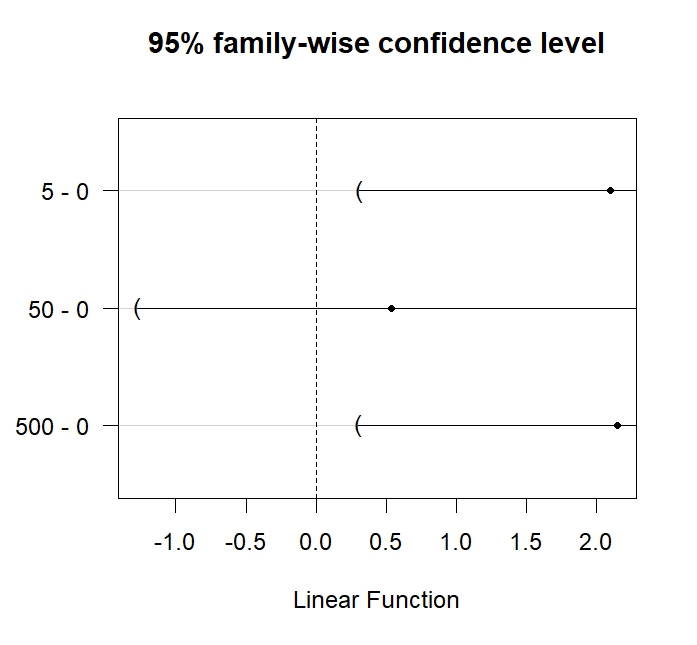
The first example uses the litter weight data in a toxicological bioassay (data available in library(multcomp)) [7]. The R-code is simple to estimate adjusted p-value or simultaneous confidence intervals
library(multcomp)
data(litter)
medrs<-tapply(litter$weight, litter$dose, median) ¯¯¯# group-specific medians
medrsV<-medrs[as.integer(litter$dose)] ¯¯¯¯¯¯¯¯¯# median for each subject
litter$tresponse<- abs(litter$weight-medrsV) ¯¯¯¯¯¯# Levene transformation
mod2<-lm(tresponse~dose, data=litter)¯¯¯¯¯¯¯¯¯¯# linear model¯
summary(glht(mod2, linfct = mcp(dose ="Dunnett"), alternative="greater"))
plot(glht(mod2, linfct = mcp(dose ="Dunnett"), alternative="greater"))
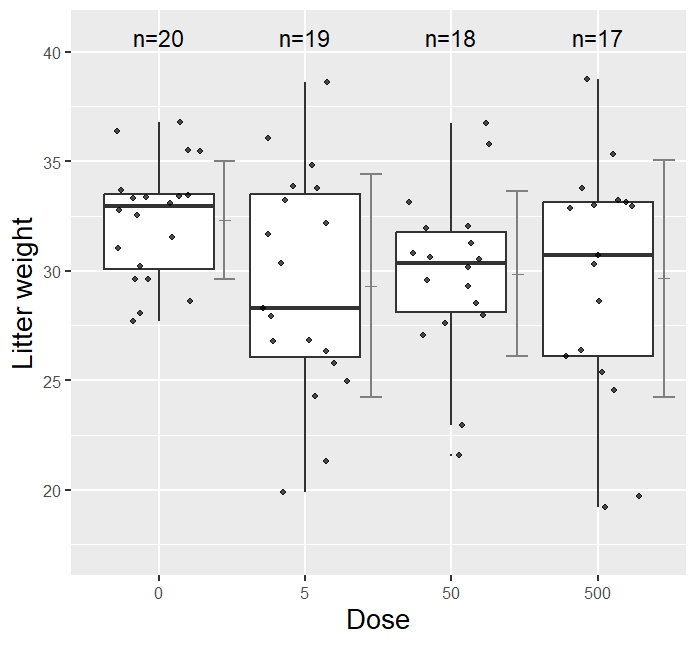
| Comparisons | p-value LevDun |
|---|---|
| 5 - 0 | 0.022 |
| 50 - 0 | 0.491 |
| 500 - 0 | 0.022 |
The second example uses the survival time data in [1] as an example for unstructured k-sample design:
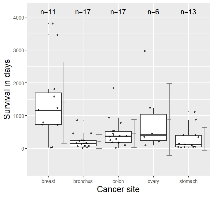
boos<-data.frame(survival, group=as.factor(grp))
library(multcomp)
medrs<-tapply(boos$survival, boos$group, median) # group-specific medians
medrsV<-medrs[(boos$group)] # median for each subject
boos$tresponse<- abs(boos$survival-medrsV) # Levene transformation
mod3<-lm(tresponse~group, data=boos)
summary(glht(mod3, linfct = mcp(group="GrandMean")))
library(GLDEX)
no0<-fun.zero.omit(boos$tresponse)
boos0<-data.frame(no0, group0=as.factor(grp0))
mod4<-lm(no0~group0, data=boos0)
summary(glht(mod4, linfct = mcp(group0="GrandMean")))
| Cancer site | LevDun | modLevDun |
|---|---|---|
| breast | 0.002 | 0.002 |
| bronchus | 0.999 | 0.13 |
| colon | 0.999 | 0.78 |
| ovary | 0.31 | 0.54 |
| stomach | 0.99 | 0.79 |
| global Levene min(p)-test | 0.002 | 0.002 |
| global Levene F-test | 0.027 | - |
The advantage of the new heterogeneity test compared to the F-test variant (in library(misty)) is obvious: not only is a global p-value is available (i.e. ’variance heterogeneity exists’), but the statement ’the variance at the tumor site=’breast’ is increased with respect to the overall variance’ is also available.
6 Summary
The proposed Levene-Dunnett test can be recommended for randomized designs with a control or placebo group for the analysis of possible variance heterogeneity, whereby the modified version should be used for small sample sizes. An analogous heterogeneity test for unstructured designs is also possible. Two data examples were used to illustrate the simple R code and the problem-adapted interpretation.
References
- [1] Dennis DB, Kaiyuan D., and Xiaoni L. Pairwise comparisons for levene-style variability parameters. Comm. Stat- B, 52(4):1562–1576, APR 3 2023.
- [2] C. W. Dunnett. A multiple comparison procedure for comparing several treatments with a control. J. Amer. Statist. Assoc., 50(272):1096–1121, 1955.
- [3] L.A. Hothorn. Comparisons of multiple treatment groups with a negative control or placebo group: Dunnett test vs. closed test procedure. arXiv:2012.04277 (2020), 2020.
- [4] Katsileros A., Antonetsis N. A comparison of tests for homoscedasticity using simulation and empirical data. Comm. Stats-A, 31(1), JAN 2024.
- [5] F. Konietschke, S. Bosiger, E. Brunner, and L. A. Hothorn. Are multiple contrast tests superior to the anova? Intern. J. Biostat., 9(1):63–73, May 2013.
- [6] Pallmann P., Hothorn LA., and Djira GD. A Levene-type test of homogeneity of variances against ordered alternatives. Comput Stat., 29(6):1593–1608, DEC 2014.
- [7] P. H. Westfall. Multiple testing of general contrasts using logical constraints and correlations. J. Amer. Statist. Assoc., 92(437):299–306, March 1997.