A non-autonomous framework for climate change and extreme weather events increase in a stochastic energy balance model
Abstract
We develop a three-timescale framework for modelling climate change and introduce a space-heterogeneous one-dimensional energy balance model. This model, addressing temperature fluctuations from rising carbon dioxide levels and the super-greenhouse effect in tropical regions, fits within the setting of stochastic reaction-diffusion equations. Our results show how both mean and variance of temperature increase, without the system going through a bifurcation point. This study aims to advance the conceptual understanding of the extreme weather events frequency increase due to climate change.
1 Introduction
The purpose of this paper is twofold: to describe a scheme for three-timescale non-autonomous dynamical system suitable for the description of climate change and to present a new example of an energy balance model (EBM) with spatial structure. This model fits into our abstract framework and may contribute to a conceptual explanation of the increase in the frequency of extreme events. The non-autonomous nature of this example is crucial, making its connection to the foundational scheme particularly interesting.
From the viewpoint of climate change analysis, our goal is to provide a simplified model that demonstrates how temperature fluctuations increase with rising carbon dioxide () concentrations. Probably the most dramatic example nowadays of climate change is the increased frequency of extreme events. As pointed out by the IPCC Report [HDG+01], this can result from both an increase in the mean temperature and an increase in the variance of temperature, as shown in Figure 1, not only by the increase of the mean value but also by the increase in the variance of a climatic variable.
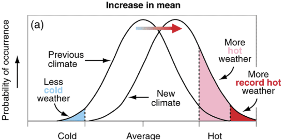
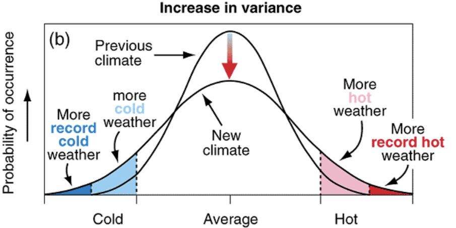
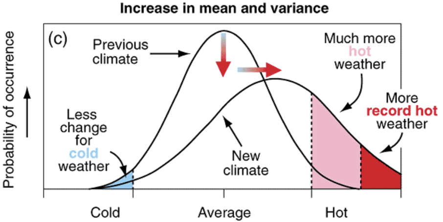
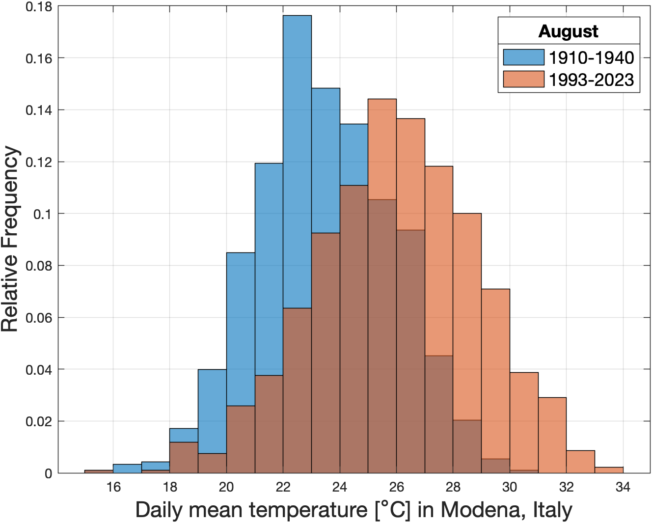
This phenomenon is not just speculative and can be observed by looking at real data, as can be done in Figure 2(a). It shows the histogram of the daily mean temperature recorded in August in two different periods, from to in blue, and from to in red. In our opinion, being able to explain the joint increase of mean value and variance is a challenging and, at the moment, a completely open question. Indeed, a classical paradigm to explain the increase in the frequency of extreme events is given by a dynamical system approaching a bifurcation point, a system subject to random fluctuations, which are amplified near the bifurcation point [DSvN+08, SBB+09, AWVC12, LL+12, GL20]. But the main question then is whether the Earth, nowadays, is close to a bifurcation point or not, an issue which is speculated but not proven. Looking to the far past, it is rather clear that bifurcations took place connecting a moderate climate like our own today with glacial climates. But a clear indication that now we are close to a new bifurcation point in the direction of a warmer climate is missing. Except for certain data near the Tropics: localised in space at that latitude, there is experimental evidence of a potential bistability and therefore of the possibility of a fast transition to a warmer climate [DG18]. But far from the Tropics, the data are different. Therefore we have developed a space-dependent model which incorporates this difference. Seen globally, as an infinite dimensional dynamical system on the whole globe, the Tropics bistability does not add a new bifurcation to the model.
We focus on the class of EBMs, which give an elementary, yet useful, representation of Earth’s climate by capturing the fundamental mechanisms governing its behaviour [Bud69, Sel69, Nor75, Ghi76, Día97, GL20, CLM+23]. This type of models, which describes temperature evolution, assumes that it evolves according to the radiation balance of the budget, i.e. the difference in the radiation absorbed and emitted by the planet. Other key factors, such as solar insolation, atmospheric composition, and surface properties, are considered in EBMs in order to get a radiation budget as accurate as possible.
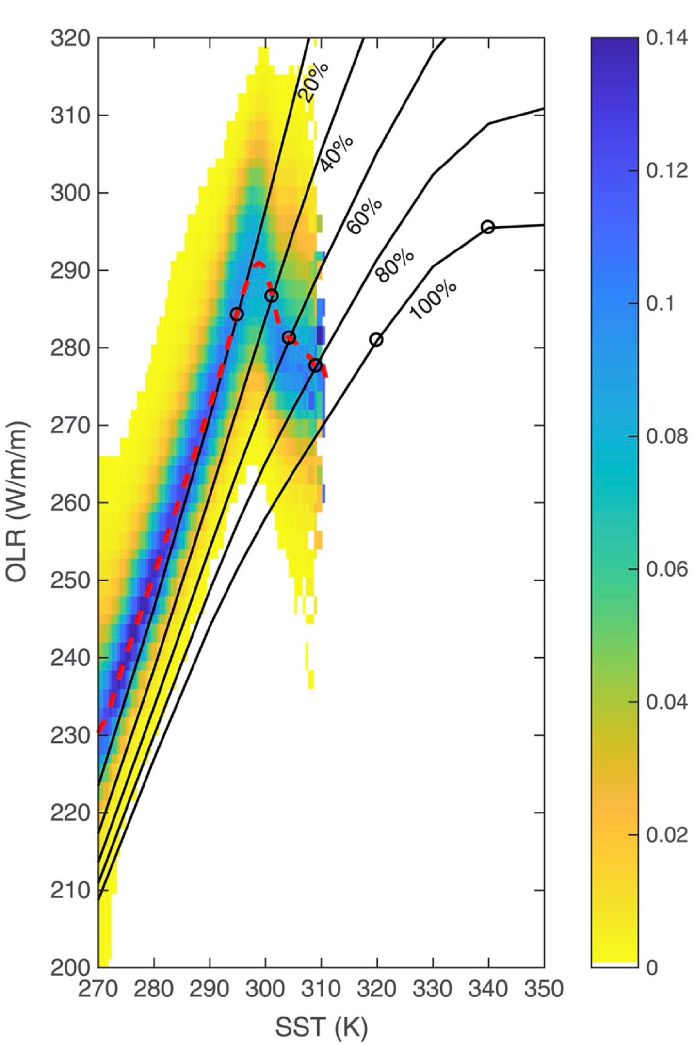
More in detail, we work with a Budyko-Sellers one-dimensional energy balance model (1D EBM), in which a diffusion term modelling meridional heat transport is added as a driver of temperature evolution [NK17]. The novelty of our model consists in adding, for the first time, a particular phenomenon that may happen at the Tropics. Indeed, one of the key mechanisms to stabilize Earth’s temperature is the Planck feedback. It consists of an increase of outgoing longwave radiation (OLR) as surface temperature increases, thanks to the Stefan-Boltzmann law. But there exist cases, and our model highlights one of them, where this feedback can fail, as in the super-greenhouse effect (SGE) [EWV14, BC16, DG18]. This phenomenon is a feedback between water vapour, surface temperature and greenhouse effect. Once the sea surface temperature or greenhouse gas concentration reaches a certain level, the increase in absorbed thermal radiation from the surface due to augmented evaporation with rising sea surface temperature (SST) outweighs the concurrent elevation in OLR, causing OLR to decline as SST increases.
From the mathematical viewpoint, the EBM proposed here is a non-autonomous stochastic partial differential Equation (SPDE) of reaction-diffusion type [DPZ96, DPZ14]. The non-autonomy stands in a slowly varying term corresponding to concentration. We clarify the link between such a scheme and a more classical adiabatic approach where the slowly varying term is kept constant and the long-term behaviour of the corresponding autonomous dynamical system is investigated. It is worth pointing out that the timescale of our model is intermediate between the daily timescale of weather and the centurial timescale of climate. It is sometimes called macroweather and it is of the order of a month to one year. For this reason, the abstract framework of a two-timescale separation of a non-autonomous dynamical system is introduced to describe the macroweather-climate dichotomy, interpreting the weather as a faster timescale than macroweather which is averaged out by looking at the temperature on time interval of months.
This paper is organized as follows. In Section 2, we introduce the non-autonomous framework for weather, macroweather, and climate, with a particular focus on the latter two. We outline the scale separation between them and provide their tentative definitions. This first, abstract part culminates in a link between macroweather and climate, justifying an adiabatic approach to studying the former in the presence of a non-autonomous dependence, such as concentration in the atmosphere. In Section 3, we begin by recalling the key concepts of EBMs, starting with the zero-dimensional version in Section 3.1. We discuss why EBMs are suitable for describing macroweather and how they can explain the increase in global mean temperature (GMT) due to rising concentrations. In Section 3.2, we introduce our new 1D EBM, detailing the parametrization of all the terms of the parabolic partial differential equation (PDE). Section 3.3 describes the deterministic properties of the model, such as the existence of one or more steady-state solutions and their dependence on the parameter. In Section 3.4, we discuss the stochastic extension of the model and its properties, including the existence of an explicit invariant measure. Section 3.5 presents the main results of the second part. We demonstrate how our model predicts an increase in the variance of temperature fluctuations under in the current climate configuration, without introducing new bifurcation points. We use both numerical tools and theoretical arguments to explain and understand this phenomenon. Finally, Section 4 summarizes our findings, while Appendix A details the finite-difference scheme used for numerical simulations and some spectral properties needed to deduce the existence of the invariant measure for the stochastic problem.
2 The non-autonomous scheme with three timescales
In Section 3 below we introduce a stochastic EBM with suitable space dependence, and a slowly varying parameter corresponding to concentration, in order to investigate the time-change of fluctuations, as discussed also in the Introduction. There are three different timescales involved in this modelling. We could skip the first one by just mentioning [Has76], and restrict ourselves to two timescales only, but at the same time we want to insist on the non-autonomous structure of the modelling, hence it is convenient to enlarge the discussion a bit.
In the modelling we have in mind there are three timescales, called:
-
•
weather, or meteo, where variations are visible at the timescale of hours/day (variables will be denoted by , etc.);
-
•
macroweather, where variations are visible at the timescale of months/year (variables will be denoted by , etc.);
-
•
climate, changing at the timescale of dozens of years (probability measures and their expected values characterize this level, still changing in time).
Subdivision and attribution of a precise timescale are not strict.
Remark 1
The reader will realize that, for the purpose of Section 3, we could start from Subsection 2.5 Let us then explain why we think that Subsections 2.1-2.4 are also very important. As already said, a main purpose of this work is to identify possible explanations for an increase in variance, when a parameter changes. In a sentence, the two main ingredients are a noise in the system equations and a suitable nonlinearity which amplifies the variations of the noise in a different way for different values of the parameter. The noise, then, is crucial. Subsections 2.1-2.4 are devoted to explaining its origin.
2.1 The weather timescale
Following [Has76], it is natural to model the weather scale by deterministic equations, ordinary equations for simplicity of notation (but the ideas are the same for PDEs); randomness can be introduced but it is not strictly necessary, except maybe for a description of the uncertainty about initial conditions and parameters, not included in the present discussion. Following [Has76], we distinguish the main physical variables in fast and slow ones, according to a system of the form
for a small . Here changes in unitary time (corresponding to hours/day), and varies very slowly (monthly, say). In addition, the slow variable is influenced by a slow time-change of structure, described by the time-varying parameters . The function is assumed to be slowly varying, hence is super-slowly varying (from here the three timescales arise).
The parameter corresponds to the typical reaction time of the slow variables, measured in the unitary time of . Appreciable changes of happen in a time of order , at the meteo-scale.
With great simplification, we may think that collects the fluid dynamic variables (the fluid Velocity plus other related variables), which are very unstable and rapidly changing at the daily level, while represents Temperature. In this case, the unit of time at the meteo level is of the order of hours, and is of the order of a few months, hence e.g. of order 100. On the contrary, the time-change of concentration, call it , is of the order of a dozen of years, hence e.g. of order 10000 in the meteo scale. With these figures, has a relaxation time of and of order .
2.2 Macroweather timescale for
Then we change the scale and set
so that we observe variations of in unitary time. We call this the macroweather timescale. It holds
Let us recall that, at this timescale, varies very slowly. Let us look for a simplification of this equation, where does not appear anymore.
2.3 The averaging approximation
Let us heuristically describe the averaging approximation, which can be made rigorous under proper assumptions for suitable systems, see [FW12].
At the integral level, we have
If is small, let us use the reasonable approximation
Then, if , we heuristically invoke an ergodic theorem and approximate
where is invariant for
Setting
we may write
and then again approximate it to
Hence we get the simplified model
2.4 Hasselmann’s proposal
However, in our case, this simplification is not realistic. If is of order , then is of order one, because we need the validity of the approximation
But on a time of order one, we observe variations of , we said above, hence the approximation
is not so strict (on the contrary, it is excellent for the approximation).
We need to keep fluctuations into account at the macroweather scale. A phenomenological way (Hasselmann proposal) is to replace the model above by
for a suitable ”volatility” (Stratonovich integral looks more appropriate). In [Has76], heuristic justifications are given, inspired for instance the random displacements of a Brownian particle in a fluid of molecules (which on their own are subject to a deterministic fast dynamics, coupled with the slow deterministic dynamic of the bigger particle). The Bremen school on Random Dynamical Systems and other research groups explored for some time rigorous justifications for this proposal, but a final answer is not known, see for instance [Arn01, Kif01]. However, the observation of temperature time series at the timescale of month-year clearly shows some form of stochasticity and thus Hasselmann’s proposal looks very appealing.
For our purposes below, adhering to Hasselmann’s proposal is essential, since our results are the consequence of random perturbations of a nonlinear system representing climate dynamics at the macroweather timescale, namely a stochastic version of the EBM. Random perturbations are often accepted just based on the generic justification of an unknown coupling with other segments of the physical system (which at the end of the story is the reason also here, namely the coupling with the fast variables) but Hasselmann’s proposal is more precise explanation.
Let us however advise the reader that we shall start, in our example below, from a stochastic PDE for the temperature macroweather-scale, given a priori, not derived precisely from the weather scale as described above. We want to concentrate on the consequences of particular nonlinearities. Our model will have the simplified form
with constant .
2.5 Macroweather and climate
As announced at the end of the last subsection, our investigation starts from an equation of the form (stochastic differential equation or SPDE)
| (1) | ||||
where we skip the subscripts but keep in mind that it is a macroweather model, we have skipped the factor but we shall choose a small diffusion coefficient , and the nonlinear function will be chosen by means of typical arguments related to EBM’s. The slowly varying function will describe the effect, in the model, of slowly varying -concentration, appreciated on a timescale of dozens of years.
The climate is a collection of statistical information from the time series of this model. If it were an autonomous system ( equal to a constant), we would invoke invariant measures. Due to the time-change in , we have to use the formalism of time-varying invariant measures. However, at the simulation level, we approximate this time-varying system by an adiabatic system parametrized by a parameter :
and investigate its invariant measures, parametrized by . The slow change of statistics for the true non-autonomous system is mimicked by the change of statistics when the parameter is changed.
Concerning precisely the concept of climate, let us introduce some formalism. We again limit ourselves to stochastic differential equations (SDEs) on an Euclidean space (e.g. the space-discretization of a stochastic partial differential equation, as in our main example below) but the concepts can be widely generalized, see for instance [FPT22] for a non-autonomous abstract random dynamical system framework related to the weather-climate dichotomy (that we improve here by introducing a third level, the macroweather). Call the set of probability measures on Borel sets of . Consider the SDE (1) on the full real line of time. Assume that is a -dimensional two-sided Brownian motion defined on a Probability space with expectation . Assume that, for the Cauchy problem on the half line with initial condition at time , with arbitrary and , at least weak global existence and uniqueness in law holds, and denote the solution by , ; assume is Borel measurable from to endowed with the weak convergence of measures.
For all introduce the Markov semigroup mapping into defined by the identity
for every and every bounded continuous test function on . One can prove that
Moreover, one can link the Markov operator for equation (1) to the Fokker-Planck equation
but we do not stress the rigorous results here.
With these notations, a time-varying invariant measure is a family
such that
Under suitable assumptions for the stochastic equations, there are results of existence (easy) and also uniqueness (more difficult) for such invariant families. This part of the theory is in progress. When the invariant measure is unique, we call it ”the climate”.
When uniqueness does not hold or it is not known, the idea could be to look for families not only invariant but also with additional properties of interest for physical sciences or other reasons. A typical one could be a pull-back version of ”convergence to equilibrium”:
| (2) |
where is a ”natural” measure, like a rotation invariant centered Gaussian measure on .
If varies very slowly, we expect that also varies accordingly, and thus an adiabatic approach to the numerical computation of is reasonable, as already remarked above.
3 Energy balance models
3.1 The macroweather timescale and the global mean temperature increase due to concentration
EBMs are elementary climate models where, in the simplest form, the temperature of the planet evolves according to the balance of the radiation absorbed and emitted by the Earth [Bud69, Sel69, Nor75, Ghi76, GL20]. Their ability to capture the essential dynamics of Earth’s climate system while remaining computationally tractable makes EBMs valuable tools for understanding a wide range of climate phenomena, from the onset of ice ages to the impacts of greenhouse gas emissions on global temperatures [DF11, BDvdH22]. There exists a spectrum of complexity for this kind of model, starting from the zero-dimensional (0D) case, moving to the one-dimensional (1D) case, and arriving at higher-dimensional models [NK17]. Before delving into the details of our 1D EBM with space heterogeneous radiation balance, we illustrate (i) why an EBM has a macroweather timescale, and (ii) why an increase of concentration in a stochastic 0D EBM leads to an increase of GMT, but not the variance of the solution.
First, we consider a 0D EBM for the global mean temperature which given a positive initial condition , is an ODE of the form
| (3) |
In this model, the radiation emitted by the planet is assumed, according to Budyko empirical radiation formula [Bud69], of the form
where are positive constants that can be derived by a best-fit estimate with real data observations; denotes the heat capacity per square meter, while and are respectively the global mean radiation and coalbedo. Lastly, the additive parameter the effect of concentration on the radiation balance [NK17, BDvdH22, DSBFK24]. Denoting by the unique stable fixed point of the model, i.e.
the solution of (3) is given by
where is the relaxation time, i.e. the timescale at which a deviation from the equilibrium temperature is reabsorbed. Considering an all-land planet, it is reasonable to consider the heat capacity as half the heat capacity at constant pressure of the column of dry air over a square meter, as pointed out in [NK17], leading to
On the other hand, satellite data suggest [NK17, GLN93]
This leads to a relaxation time of the other of one month, as
It is worth pointing out that the hypothesis of an all-land planet is a huge simplification of reality. Indeed, the Earth’s system has various components capable of storing heat efficiently, each with its own unique capacity [GL20]. The value for we have considered corresponds to the capacity of the atmospheric column. But, even considering a planet with a mixed-layer only ocean, the heat capacity would be times larger ([NK17]), i.e. in the order of a few years, remaining thus in the macro weather timescale.
Second, we force the model with a stochastic noise modelling the effect of fast terms with respect to the slow radiation balance terms of equation (3). Denote by a Brownian motion, and consider the SDE given by:
| (4) |
where is the noise intensity. Denoting by the solution can be explicitly written, using a variation of parameters technique ([Bal17]) as
The solution is a Gaussian process with a mean value
| (5) |
and variance
| (6) |
Further, the stochastic EBM in (4) has a unique gaussian invariant measure , whose mean and variance , can be obtained taking the limit for the time that tends to infinity in (5) and (6), leading to
Thus, a change in the concentration leads to a change in the mean value of the climate, i.e. the invariant measure, but not in its variability. Usually, the variability increase results from a critical transition, such as a saddle-node bifurcation, which arises in the model. This is the concept of bifurcation-induced tipping point, which leads to the critical slowing down behaviour of the system, resulting in an increase of variance and autocorrelation close to the bifurcation point [DSvN+08, SBB+09, AWVC12, LL+12]. However, the presence of a bifurcation point for the global scale climate is questionable, and the presence of bistable regimes for climate components, sometimes called tipping elements such for Atlantic meridional overturning circulation or polar ice sheets, is localized in space. For all these reasons, in the next section, we will describe a new one-dimensional model with a local in-space change in the non-linear term that is able to explain the variance increase.
3.2 Model formulation
In this section, we propose a 1D EBM with space-dependent radiation balance with local bistability in the outgoing radiation term. The new term does not lead to the addition of a new bifurcation in the model, even if results in a non-linear change in the global mean temperature w.r.t. concentration, in comparison with a linear increase in the case of the non-space dependent emitted radiation case. However, by adding a noise component to the model, we detect an increase of fluctuations over time for those values of concentration in which the non-linear behaviour of GMT is triggered. We connect the increase in fluctuations over time, that we denote time variance, to a local (in space) notion of relaxation time. The latter indicator in a sense gives information about the local stability of a space point for, in our case, a global stable temperature configuration.
The main characteristics of a 1D EBM are that the temperature , depending on time and space , where denotes latitude, are that it evolves according to the diffusion of heat, and the planet energy balance [Bud69, Sel69, Ghi76, CLM+23]. Our model, which is an extension of the one considered in [DSBFK24], assumes that the temperature satisfies the non-linear parabolic partial differential equation (PDE)
| (7) |
The heat capacity is considered uniform over the whole planet, which we assume is an all-land planet, as the one presented at the beginning of Section 3. The PDE is a reaction-diffusion type [Tem97, Smo12]. In the following, we are going to describe the terms governing its time evolution, while the values of the constants appearing in the parametrizations can be found in Table 1.
In scientific modelling, heat diffusion is often depicted assuming the planet as a thin shell. This leads to a non-constant diffusion coefficient of the form , with , where the term arises due to the spherical setting [NK17, Chapter 5]. However, this choice introduces difficulties for the mathematical treatment, resulting in degenerate problems [Flo14, CMM20]. For instance, proving the existence of steady-state solutions requires the use of weighted Sobolev spaces. To address this issue, we introduce a simplifying perturbation that removes the singularity at the border [DSBFK24]. We consider the diffusion function given by:
with and , if , even and non-decreasing in . The radiation absorbed by the planet, denoted as , is the product of a spatially dependent solar radiation function , where , and a temperature-dependent co-albedo . The co-albedo , where is parameterized by a smooth, non-increasing, bounded function [BDvdH22, DSBFK24]
| (8) |
with , denotes ice albedo, denotes water albedo, , and is a parametrization constant.
Third, we describe the modelization of the radiation emitted , which is the main innovation of our model. Local bistability in the Outgoing Longwave Radiation (OLR) may arise in tropical regions due to a positive feedback loop involving surface temperature and moisture. This feedback, above a threshold of sea level pressure and GHG concentration, causes the atmosphere to become optically thick, thus reducing OLR [DG18].
To model this effect, we choose a space-dependent, latitude-symmetric Outgoing Longwave Radiation (OLR) of the form:
| (9) |
where and denote respectively the OLR at the pole and the equator. The convex combination between and Figure 3 shows the space-dependent , using different colours to represent distinct latitude points.
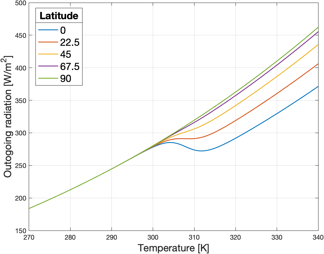
We define them as:
| (10) |
where is the emissivity constant, is the Stefan-Boltzmann constant. On the other hand, at the poles, we reproduce the super-greenhouse effect by considering:
| (11) |
where is a smooth transition function of the form
where K and are respectively a reference temperature and a constant in the transition velocity involved in the SGE parametrization. Further, is an emissivity constant at the equator taking into account the OLR reduction due to the SGE. Note that the OLR at the poles and at the equator in (10)-(11) has been defined, just for mathematical convenience, in the physical meaningless range of negative Kelvin temperature.
Lastly, the additive positive parameter models the effect of concentration on the energy budget [MMS01, BDvdH22]. A higher leads to lower radiation emitted back to space from the surface. We emphasize the reason behind considering a constant value for the parameter . Greenhouse gas concentration can be regarded as constant at a macroweather, i.e., monthly, timescale, by avoiding seasonality insertion since it evolves on a much larger timescale. For instance, the concentration has increased by around from to , moving from parts per million (ppm) to ppm [oCCI23]. In a first approximation, we assume that the spatial distribution of greenhouse gases is uniform over the globe. This assumption, although no longer the state of the art, was widespread at the turn of the century and is based on the well-mixing property of GHG. This means that since most GHGs, such as , have a large lifetime, many studies have been conducted using global average values for the spatial distribution [MHSS98, MMS01, HDG+01].
| Symbol | Meaning | Value |
|---|---|---|
| Diffusivity constant | ||
| Mean solar radiation | ||
| Emissivity at the poles | ||
| Emissivity at the equator | ||
| Boltzmann’s constant | ||
| Ice albedo | ||
| Water albedo | ||
| Constant rate - albedo parametrization | ||
| Constant rate - SGE parametrization | ||
| Reference temperature - albedo parametrization | ||
| Reference temperature - SGE parametrization | ||
| Heat capacity |
3.3 Deterministic properties of the model
In this section, we describe the deterministic properties of our model, as the number of steady-state solutions and their stability. The new feature of our model is the rise of a strong non-linear increase of GMT with respect to the greenhouse parameter , in the proximity of the model configuration describing the actual climate of the Earth.
In general, in dynamical system theory, huge information are given by the study of the steady-state solutions of the model, which are, in a sense, the long-time behaviour solutions. More in detail, four our model consists of the non-negative solutions of the following elliptic PDE:
| (12) |
A common way to prove the existence of at least one stable steady-state solution involves a variational approach by studying the minimization problem
| (13) |
where:
| (14) |
with and denoting the Sobolev space of order and exponent [Nor75, NHPW79, Nor90, Bre11]. Applying the results [DSBFK24, Theorem 1 and Theorem 1], it is possible to gain information about the existence and uniqueness of a steady state solution.
Proposition 2
Note how the second part of the previous result gives qualitative information on the behaviour of the GMT. Furthermore, if the diffusion coefficient is sufficiently large and the 0D EBM, obtained by removing the diffusion term and averaging in space the radiation balance, is bistable, it can be rigorously proven the existence of a second stable steady-state solution and a third unstable one [DSBFK24, Theorem 2].
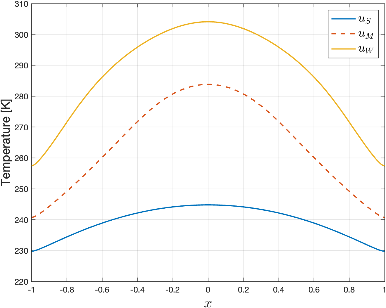
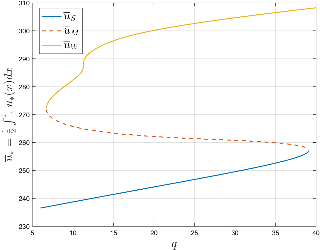
Given the non-linear nature of the problem, a rigorous demonstration of all properties of the model is not always possible. In this case, the problem can be overcome by using numerical simulations. In particular, for each fixed , we numerically simulated the solutions of (12). As varies, we obtained, according to the large literature on this kind of model, that there can be either 1 or 3 stationary solutions. In the former case, the solution is stable. In the latter case, two solutions are stable, one describing a ”snowball” configuration for Earth’s temperature with ice all over its surface. The other describes a warm climate , similar to the one in which we are living. Additionally, an unstable solution , whose average global mean temperature (GMT) lies between the GMT of and also arises. See Figure 4(a) for a graphical representation of the steady-state solutions in the bistable case.
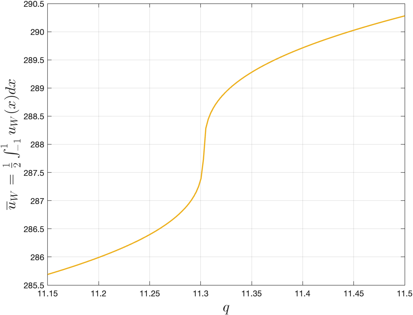
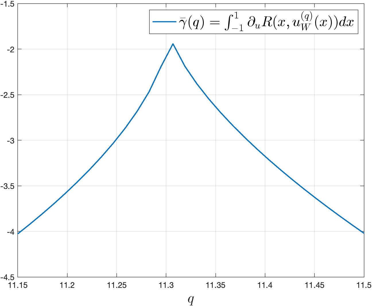
In general, proving theoretically the results for such kinds of models is non-trivial due to the presence of nonlinear terms in the energy budget parametrization. The bifurcation diagram of the model in the plane, where denotes a solution of the elliptic PDE, and is its GMT, is depicted in Figure 4(b). We highlight how the addition of a space-dependent OLR with tropics bistability does not introduce a new bifurcation. Thus, no new steady-state solutions are added or the stability of the already existing ones is altered. However, as highlighted in Figure 4(c), a strong non-linear behaviour of the GMT for the warm solution appears for the value of in the neighbourhood of , a thing that does not happen if we remove the bistability in [DSBFK24]. Our aim is to focus on that phenomenon, when a noise component, describing the weather effect is added to the model. This is the main topic of the next section.
3.4 Stochastic properties of the model
As discussed in the previous paragraphs, the EBM presented in this work corresponds to a macroweather timescale. However, as far as it has been introduced, it lacks in taking into account the effect of fast components of Earth’s system, such as atmospheric pressure, wind, and precipitation. In literature, this has been achieved in an elementary way by adding a stochastic term, such as white noise, to the radiation budget [Has76, Imk01, DLV09, DD22]. Note that this addition is necessary to describe the increase in the frequency of rare events. In fact, while a deterministic EBM is useful for obtaining information on global mean temperature, it is not able to investigate fluctuations around it due to all phenomena, such as weather, not included in the radiation balance of the model.
We consider and the stochastic EBM given by:
| (15) |
where denotes a cylindrical Wiener process on , is a non-negative initial condition and is the operator
| (16) |
We would like to apply the invariant measure theory for gradient systems to deduce the existence, and uniqueness of an invariant measure and its explicit formula. This can not be applied to the operator since it is invertible on For this reason, we consider the operator
| (17) |
where is a positive constant. By exploiting the Sturm-Liouville theory, it can be proved that is a self-adjoint, negative definite operator, with eigenvalue , such that the trace of , for some . See Appendix A.2 for a sketch of the proof of these facts. In this way, it is possible to deduce the following result [DP06, DPZ14, DSBFK24].
Proposition 3
Let Then, there exists an unique -a.s. -valued mild solution of the SPDE (15). Further, there exists an unique Gibbs invariant measure , and with explicit formula
| (18) |
where and
We remark that the invariant measure is the object, in our context of stochastic EBM, that in Section 2.5 has been taken as the definition of climate. Then, it is worth pointing out the link between the invariant measure and the functional building up the variational problem (13). Indeed, at least formally, we can write the Gaussian measure as
where is a normalization constant, is the covariance operator of , denotes the scalar product on and is the formal notation for the Lebesgue measure on . By an integration of parts, we deduce
Hence, substituting back the formal expression for in (18), we conclude
From this expression, we can deduce two important facts. First, the invariant measure of the stochastic EBM is concentrated on the global minimum points of the functional . Second, the study of and its spread depending on is as difficult as understanding how the functional changes. For this reason, in the next section, we will use numerical simulation to investigate how changes, depending on the adiabatic parameter , as the lies in the critical interval in Figure 4(c).
3.5 Variance and extreme weather events increase
It is widely acknowledged that greenhouse gas emissions from human activities have led to more frequent and intense weather and climate extremes since the pre-industrial era, particularly temperature extremes [oCCI23]. Despite numerous definitions proposed to assess what constitutes an extreme event, there is currently no universally accepted definition [SDM08]. One commonly used definition considers an extreme weather event as one that exceeds a predefined threshold for a climate variable.
As it is well understood that such occurrences become more likely as the variance of that climate variable increases, we consider the time variance as a proxy indicator of extreme weather events for our EBM setting. As explained in Section 3.4, an explicit formula for the invariant measure of the stochastic EBM (4) exists. However, due to the presence of a non-linear term inside the Gibbs factor in (18), obtaining theoretical information is challenging. Thus, we rely on numerical simulations to capture the behaviour of the variance.
Specifically, given a fixed value of and the warm steady-state solution , we numerically integrate the stochastic PDE:
| (19) |
The simulation runs for years to capture the properties of the invariant measure around the warm climate , and we chose a noise intensity The finite difference method applied to simulate the equation is detailed in Appendix A.1. Here, we describe what we mean by variance, its properties detected by numerical experiments, and our observations.
Given a space point and a realization of the solution of the equation (19), we consider the variance of the process . We denote the numerical approximation of the solution by , where , and and represent the spatial and temporal meshes, respectively, over the domain and . The time-variance is calculated as
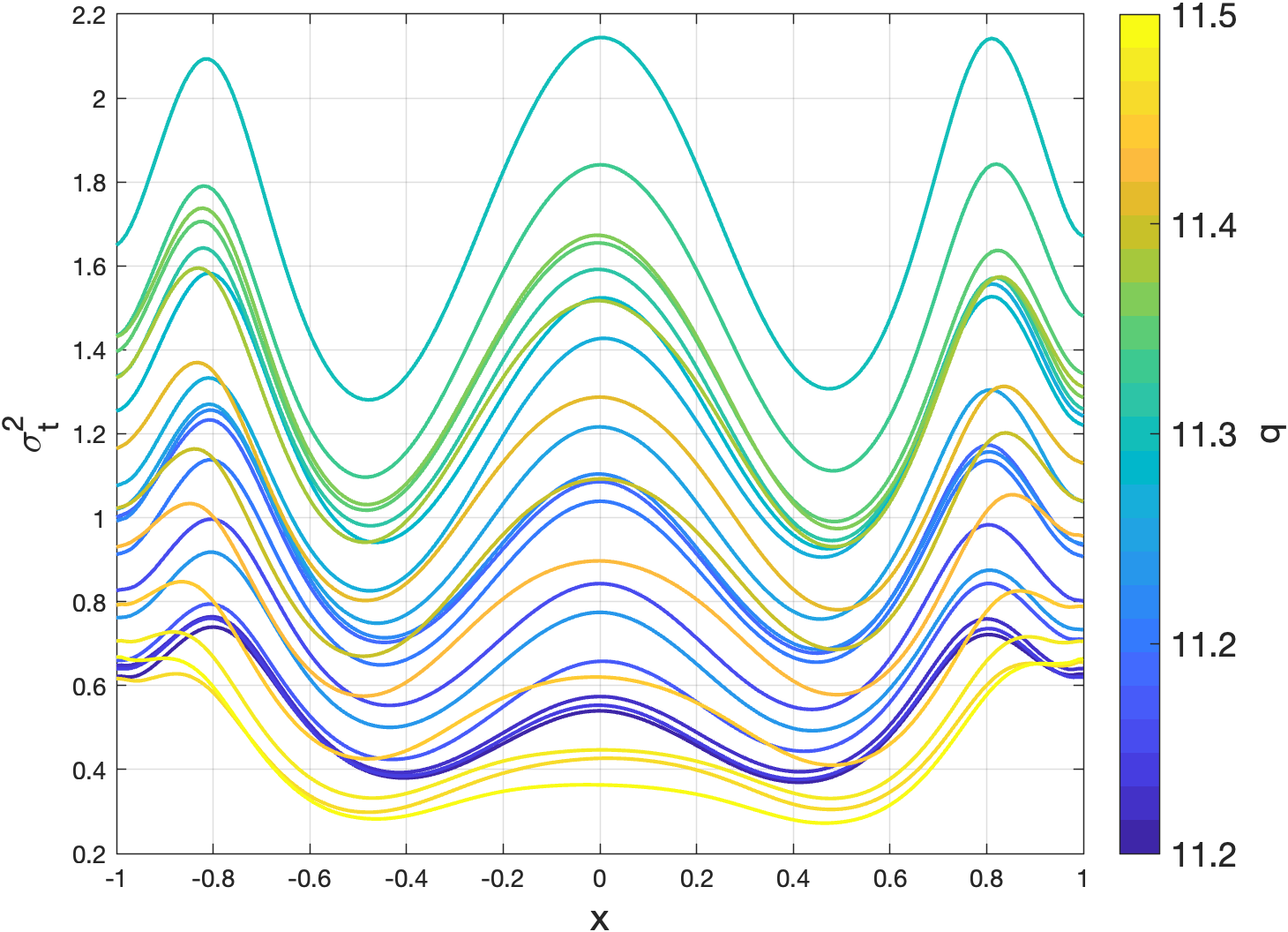
where . Figure 5(a) illustrates the time-variance indicator, with different colours representing different values of the parameter .
We observe two distinct behaviours of the variance. First, depending on , there is an increase in , peaking around , followed by a decrease. This peak corresponds to the value that results in the largest increase in GMT, as shown in Figure 4(c). Second, as expected, for a given value of , the spatial profile of is symmetric with respect to . Additionally, three local maximum points emerge one at and the others at . Our interpretation is that identifies the highest fluctuating regions as those where the freezing water temperature is crossed (sub-arctic regions, ), or where the SGE triggers bistability (tropical areas, ).
To support this interpretation, it is useful to introduce the local stability indicator
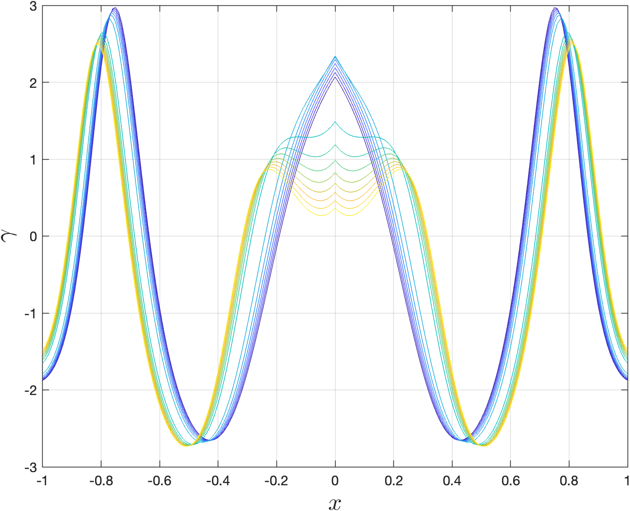
where . If the model were a simple Ordinary Differential Equation (ODE) without the coupling diffusion term, would be the eigenvalue obtained by linearizing the reaction term around the stable steady-state temperature . Positive values of indicate local instability, while negative values indicate stability if the diffusion term is removed. Figure 5(b) presents the local stability indicator , with colours denoting different values of the parameter . Notably, there is a clear relationship between time-variance and the local stability indicator: regions with high time-variance coincide with areas of positive . This explains the spatial profile of for a fixed value of .
The reason for at some points is due to the presence of the diffusion term. If , then is not a minimizer of , but instead solves the problem
| (20) |
where . Here, , and since is a minimum point, it follows . But with , no longer satisfies (20), but instead is a minimizer of , where the diffusion term appears in the second term on the right-hand side of (14). This term, which intuitively minimizes the temperature gradient, allows for some points to fluctuate around a mean value that would be unstable if .
To understand why, given , the map increases until around and then decreases, we offer the following explanation. As increases, the temperature of the warm climate increases, as can be checked by numerical simulations and partially understandable from Proposition 2. This leads the temperature, especially in the tropical area, to approach the region where instability due to the SGE arises. Once the tropical temperature surpasses this region, the instability, and thus the variance, decreases. We support our statements as follows.
-
(i)
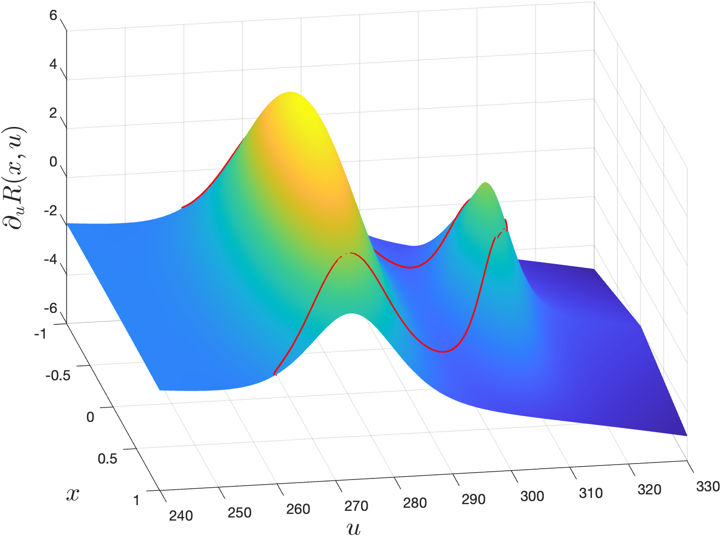
Figure 6 shows how the steady-state solution approaches unstable areas, defined by points where . For , , and , the map is presented, with the curve depicted in red. When the time variance peaks (i.e., ), the steady-state solution values around the equator are close to the local maximum of , approximately close to . For and , the equatorial steady-state value is smaller and larger than , respectively.
-
(ii)
We consider the local mean stability indicator
Its plot is shown in Figure 7(a). Although providing only average information, it exhibits behaviour qualitatively similar to that of for each fixed value of , peaking around .


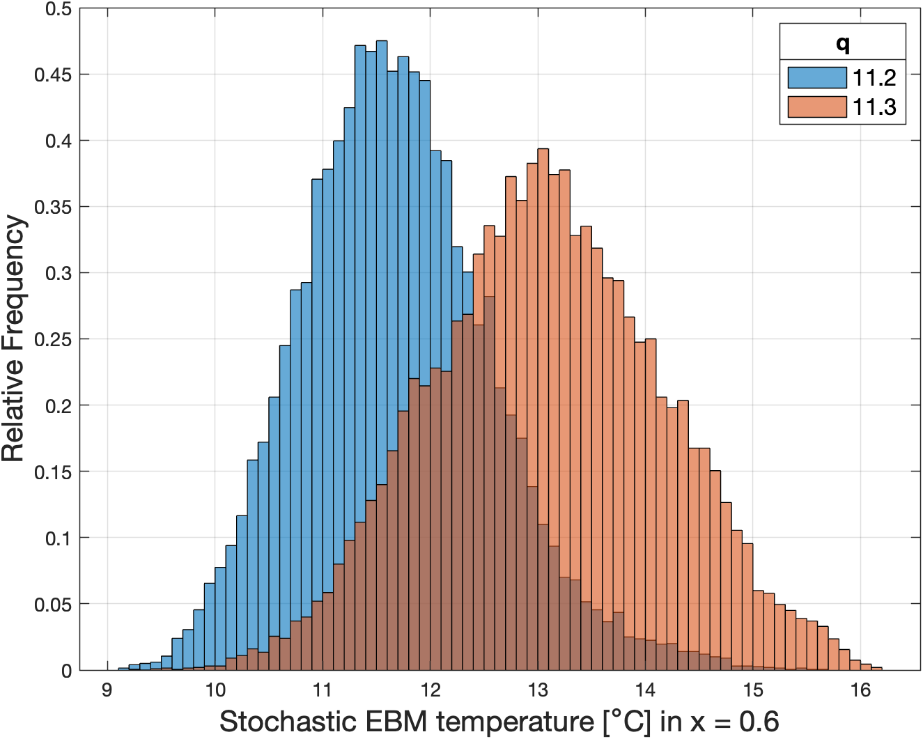
Finally, we show the distribution of the solution of the stochastic 1D EBM (4) for the fixed space point (similar results are observed for different space points). Figure 7(b) shows the distribution as a histogram, comparing two distinct values of . Blue depicts the results for , while red shows . From the plot, we deduce that our model captures the shift in the mean value and the increase in variance, correlating with the IPCC schematic climate change reproduction in Figure 1 and weather observations in Modena in Figure 2(a).
4 Conclusions
In the first part of this work, we have presented a non-autonomous framework to describe the scale separation between weather, macroweather, and climate. According to Hasselmann’s proposal, weather is conceptualized as arising from a set of deterministic equations, describing variables such as temperature on a fast timescale, typically from an hour to one day. Macroweather, on the other hand, encompasses variations that are neither as short-term as weather nor as long-term as climate. We assume that temperature on a macroweather timescale satisfies a stochastic equation, reflecting the most original aspect of Hasselmann’s work. Additionally, at the macro weather timescale, we include a non-autonomous term to model the atmospheric concentration, which evolves on a timescale of years. Finally, we identify climate with the invariant measure arising from the stochastic equation at the macro weather level.
In the second part, we have introduced a new 1D EBM on a macroweather timescale which can predict the increase in the number of extreme weather events associated with climate change. The novelty of our model relies on the parametrization in the non-linear space-dependent radiation budget. Indeed, we have inserted the presence of the SGE, a phenomenon typical of tropical areas that may lead to an instability in the OLR. Our model includes a non-autonomous term , that in light of the first part, we have considered constant, that is the effect of the concentration on the radiation balance. We have recalled the basic mathematical properties of our model, such as the existence of steady-state solutions, using also numerical simulations. Also, we have shown how the GMT of the steady state solution increases with increasing concentration. Third, we have the stochastic version of our 1D EBM, obtained by perturbing our model with an additive space-time white noise. Being in the class of stochastic reaction-diffusion SPDE, it is possible to write explicitly the invariant measure as a Gibbs one. However, the presence of the non-linearity arising from the radiation budget prevents us from deducing more information from the invariant measure.
The most important results of our work are presented in Section 3.5. There, we have exploited numerical simulations to study the changes in the invariant measure as the concentration increases. To obtain this, we have performed numerical integration of the stochastic 1D EBM on a time interval of years and with the initial condition the warm steady-state solution of the deterministic 1D EBM, changing only in different runs of the simulation. Given , for each space point we associate the extreme weather event frequency with the time variance of a trajectory of the stochastic 1D EBM at point . We explain the spatial behaviour of , which presents two local maximum points for and on for , combining heuristic reasoning with empirical indicators. The informal explanation is that the presence of the diffusion term forces the stable warm stationary solution, and the oscillations around it due to noise, to take on values that are not stable if we were to consider the ODE obtained by removing the diffusion term. These regions of temperature, which are locally unstable, correspond to the areas where the variance is highest. We also motivated the behaviour of concerning q, at fixed x. The variance observed in this way increases to a maximum value and then decreases. This is explained by the increase in GMT due to q and the presence of the diffusion term, leading the solution of the stochastic EBM to be increasingly in, and then out of, the region of instability due to the SGE.
Lastly, we are aware that our model, although based on physical laws, is largely phenomenological. In some parts of our model, we have included simplifications of convenience, such as in the perturbation of the diffusion function, which makes the problem non-singular and thus easier to deal with mathematically; in other parts, such as in the parameterisation of the space-dependent and tropic-restored OLR, we have followed the principle of simplicity. Other choices would certainly have been possible, but the elementary nature of the model leads us to avoid choices that are too fine or complex.
Concerning open questions, an important one would be understanding the correct form of the noise term. We have assumed it to be additive and without correlation in space and time. This is an extreme simplification, which allows us to deduce certain properties of the invariant measure. But already Hasselmann in his seminal work proposed a different, i.e. multiplicative, type of noise. In addition to this, understanding how the properties of the model change if more physical processes are considered, as advection, is a problem we would like to address in the future, as well as the extension of our work to a two-dimensional setting.
Appendix A Appendix
A.1 Numerical scheme
In this section, we describe the numerical method adopted to approximate the solutions of the stochastic PDE (19). We used an implicit Euler-Maruyama method, which is a small modification of the semi-implicit Euler-Maruyama method presented in [LPS14, Section 10.5].
First of all, it is worth recalling that the numerical experiments presented in Section 3.5 are all performed for a fixed value of , and using as initial condition of the parabolic stochastic problem (19). The steady-state solution solves the elliptic problem (12). To numerically approximate it, we have applied the same finite difference scheme described in [DSBFK24, Appendix A].
Second, we move to describe the numerical method for the parabolic problem. We denote by the non-linear radiation budget, and the underline notation to denote a vector (e.g. We consider two uniform meshes for the spatial domain and the time domain , i.e.
and
The number of points in the space and time mesh, respectively and , are chosen in a way that . Then, the solution to the problem can be approximated by considering the system
where are ghost points, is a collection of independent identically distributed (i.i.d.) normal random variables, and Since and , the previous system of equation can be rewritten as
where denotes the identity matrix , , , , denotes a set of i.i.d. normal random vectors, and is the tridiagonal matrix
Thus, given the numerical approximation at time , to advance the scheme at time it is needed to solve the previous non-linear system of algebraic equations. To do this, we apply the Newton-Raphson Method (NRM), that we recall in the following. We consider the map
To approximate the vector such that , the NRM consider the following sequence
where is the Jacobian matrix of with respect to Since the noise intensity is small, we expect that the choice is a good initial guess of the solution. The iteration of the NRM are stopped when .
A.2 Spectral properties of the operator
To apply the invariant measure theory, the operator defined in Section 3.4 should satisfies the following assumptions [DP06, Section 11]:
-
(i)
is self-adjoint and there exists such that
-
(ii)
There exists such that .
We denote by the eigenvalues of , where
| (21) |
Since is a Sturm-Liouville regular operator, classical results assure the existence of the real eigenvalues , and furthermore, it can be proved
First, to check hypothesis (i) it is thus sufficient to prove that
Indeed, by definition of eigenvalue, there exists an eigenfunction such that
Multiplying the previous identity by and integrating over the domain , we get
Performing an integration by parts on the left-hand side, we deduce
In conclusion,
and our claim follows from the fact that on .
Second, the hypothesis (ii) is a consequence of the following asymptotic estimate for regular Sturm-Liouville problems [FP94, Section 4]: there exist and such that
Code and data availability
This work does not include any externally supplied code. All material in the text and figures was produced by the authors using standard mathematical and numerical analysis tools. The code for the numerically simulation of the 1D EBM is available at Zenodo (https://doi.org/10.5281/zenodo.11609953). The Modena temperature data were provided by the Geophysical Observatory of Modena, University of Modena and Reggio Emilia, Italy (www.ossgeo.unimore.it) and are available upon request from the corresponding author.
Acknowledgments
We acknowledge fruitful discussions with Paolo Bernuzzi and Giulia Carigi. The research of G.D.S. is supported by the Italian national interuniversity PhD course in sustainable development and climate change. The research of F.F. is funded by the European Union (ERC, NoisyFluid, No. 101053472). Views and opinions expressed are however those of the authors only and do not necessarily reflect those of the European Union or the European Research Council. Neither the European Union nor the granting authority can be held responsible for them.
References
- [Arn01] Ludwig Arnold. Hasselmann’s program revisited: the analysis of stochasticity in deterministic climate models. In Peter Imkeller and Jin-Song von Storch, editors, Stochastic Climate Models, pages 141–157, Basel, 2001. Birkhäuser Basel.
- [AWVC12] Peter Ashwin, Sebastian Wieczorek, Renato Vitolo, and Peter Cox. Tipping points in open systems: bifurcation, noise-induced and rate-dependent examples in the climate system. Philosophical Transactions of the Royal Society A: Mathematical, Physical and Engineering Sciences, 370(1962):1166–1184, Mar 2012.
- [Bal17] Paolo Baldi. Stochastic Calculus. Springer International Publishing, 2017.
- [BC16] Tom Beucler and Timothy W. Cronin. Moisture-radiative cooling instability. Journal of Advances in Modeling Earth Systems, 8(4):1620–1640, 2016.
- [BDvdH22] Robbin Bastiaansen, Henk A Dijkstra, and Anna S von der Heydt. Fragmented tipping in a spatially heterogeneous world. Environmental Research Letters, 17(4):045006, mar 2022.
- [Bre11] Haim Brezis. Functional analysis, Sobolev spaces and partial differential equations, volume 2. Springer, 2011.
- [Bud69] Mikhail I Budyko. The effect of solar radiation variations on the climate of the earth. tellus, 21(5):611–619, 1969.
- [CLM+23] P. Cannarsa, V. Lucarini, P. Martinez, C. Urbani, and J. Vancostenoble. Analysis of a two-layer energy balance model: Long time behavior and greenhouse effect. Chaos: An Interdisciplinary Journal of Nonlinear Science, 33(11):113111, 11 2023.
- [CMM20] Piermarco Cannarsa, Martina Malfitana, and Patrick Martinez. Parameter determination for energy balance models with memory. Mathematical Approach to Climate Change and its Impacts: MAC2I, pages 83–130, 2020.
- [DD22] Gregorio Díaz and Jesús Ildefonso Díaz. Stochastic energy balance climate models with legendre weighted diffusion and an additive cylindrical wiener process forcing. Discrete and Continuous Dynamical Systems - S, 15(10):2837–2870, 2022.
- [DF11] Dietmar Dommenget and Janine Flöter. Conceptual understanding of climate change with a globally resolved energy balance model. Climate Dynamics, 37(11–12):2143–2165, March 2011.
- [DG18] M. Dewey and C. Goldblatt. Evidence for radiative-convective bistability in tropical atmospheres. Geophysical Research Letters, 45(19):10,673–10,681, 2018.
- [Día97] Jesús Ildefonso Díaz. On the mathematical treatment of energy balance climate models. In Jesús Ildefonso Díaz, editor, The Mathematics of Models for Climatology and Environment, pages 217–251, Berlin, Heidelberg, 1997. Springer Berlin Heidelberg.
- [DLV09] J.I. Díaz, J.A. Langa, and J. Valero. On the asymptotic behaviour of solutions of a stochastic energy balance climate model. Physica D: Nonlinear Phenomena, 238(9):880–887, 2009.
- [DP06] Giuseppe Da Prato. An Introduction to Infinite-Dimensional Analysis. Springer Berlin Heidelberg, 2006.
- [DPZ96] G. Da Prato and J. Zabczyk. Ergodicity for Infinite Dimensional Systems. London Mathematical Society Lecture Note Series. Cambridge University Press, 1996.
- [DPZ14] Giuseppe Da Prato and Jerzy Zabczyk. Stochastic Equations in Infinite Dimensions. Cambridge University Press, April 2014.
- [DSBFK24] G. Del Sarto, J. Bröcker, F. Flandoli, and T. Kuna. Variational techniques for a one-dimensional energy balance model. Nonlinear Processes in Geophysics, 31(1):137–150, 2024.
- [DSvN+08] Vasilis Dakos, Marten Scheffer, Egbert H. van Nes, Victor Brovkin, Vladimir Petoukhov, and Hermann Held. Slowing down as an early warning signal for abrupt climate change. Proceedings of the National Academy of Sciences, 105(38):14308–14312, 2008.
- [EWV14] Kerry Emanuel, Allison A. Wing, and Emmanuel M. Vincent. Radiative-convective instability. Journal of Advances in Modeling Earth Systems, 6(1):75–90, 2014.
- [Flo14] Giuseppe Floridia. Approximate controllability for nonlinear degenerate parabolic problems with bilinear control. Journal of Differential Equations, 257(9):3382–3422, 2014.
- [FP94] C.T. Fulton and S.A. Pruess. Eigenvalue and eigenfunction asymptotics for regular sturm-liouville problems. Journal of Mathematical Analysis and Applications, 188(1):297–340, 1994.
- [FPT22] Franco Flandoli, Umberto Pappalettera, and Elisa Tonello. Nonautonomous attractors and young measures. Stochastics and Dynamics, 22(02):2240003, 2022.
- [FW12] Mark I. Freidlin and Alexander D. Wentzell. Random Perturbations of Dynamical Systems. Springer Berlin Heidelberg, 2012.
- [Ghi76] Michael Ghil. Climate stability for a sellers-type model. Journal of Atmospheric Sciences, 33(1):3 – 20, 1976.
- [GL20] Michael Ghil and Valerio Lucarini. The physics of climate variability and climate change. Rev. Mod. Phys., 92:035002, Jul 2020.
- [GLN93] Charles E Graves, Wan-Ho Lee, and Gerald R North. New parameterizations and sensitivities for simple climate models. Journal of Geophysical Research: Atmospheres, 98(D3):5025–5036, 1993.
- [Has76] K. Hasselmann. Stochastic climate models part i. theory. Tellus, 28(6):473–485, 1976.
- [HDG+01] J. T. Houghton, Y. Ding, D. J. Griggs, M. Noguer, P. J. van der Linden, X. Dai, K. Maskell, and C. A. Johnson, editors. Climate Change 2001: The Scientific Basis. Contribution of Working Group I to the Third Assessment Report of the Intergovernmental Panel on Climate Change, 2001.
- [Imk01] Peter Imkeller. Energy balance models — viewed from stochastic dynamics. In Peter Imkeller and Jin-Song von Storch, editors, Stochastic Climate Models, pages 213–240, Basel, 2001. Birkhäuser Basel.
- [Kif01] Yuri Kifer. Averaging and climate models. In Stochastic climate models, pages 171–188. Springer, 2001.
- [LL+12] T. M. Lenton, V. N. Livina, V. , E. H. van Nes, and M. Scheffer. Early warning of climate tipping points from critical slowing down: comparing methods to improve robustness. Philosophical Transactions of the Royal Society A: Mathematical, Physical and Engineering Sciences, 370(1962):1185–1204, 2012.
- [LPS14] Gabriel J. Lord, Catherine E. Powell, and Tony Shardlow. An Introduction to Computational Stochastic PDEs. Cambridge Texts in Applied Mathematics. Cambridge University Press, 2014.
- [MHSS98] Gunnar Myhre, Eleanor J. Highwood, Keith P. Shine, and Frode Stordal. New estimates of radiative forcing due to well mixed greenhouse gases. Geophysical Research Letters, 25(14):2715–2718, July 1998.
- [MMS01] Gunnar Myhre, Arne Myhre, and Frode Stordal. Historical evolution of radiative forcing of climate. Atmospheric Environment, 35(13):2361–2373, 2001.
- [NHPW79] Gerald R. North, Louis Howard, David Pollard, and Bruce Wielicki. Variational formulation of budyko-sellers climate models. Journal of Atmospheric Sciences, 36(2):255 – 259, 1979.
- [NK17] Gerald R. North and Kwang-Yul Kim. Energy Balance Climate Models. Wiley, August 2017.
- [Nor75] Gerald R. North. Theory of energy-balance climate models. Journal of Atmospheric Sciences, 32(11):2033 – 2043, 1975.
- [Nor90] Gerald R. North. Multiple solutions in energy balance climate models. Global and Planetary Change, 2(3):225–235, 1990.
- [oCCI23] Intergovernmental Panel on Climate Change (IPCC). Climate Change 2021 – The Physical Science Basis: Working Group I Contribution to the Sixth Assessment Report of the Intergovernmental Panel on Climate Change. Cambridge University Press, 2023.
- [SBB+09] Marten Scheffer, Jordi Bascompte, William Brock, Victor Brovkin, Stephen Carpenter, Vasilis Dakos, Hermann Held, Egbert Nes, Max Rietkerk, and George Sugihara. Early-warning signals for critical transitions. Nature, 461:53–9, 10 2009.
- [SDM08] David B Stephenson, HF Diaz, and RJ Murnane. Definition, diagnosis, and origin of extreme weather and climate events. Climate extremes and society, 340:11–23, 2008.
- [Sel69] William D. Sellers. A global climatic model based on the energy balance of the earth-atmosphere system. Journal of Applied Meteorology and Climatology, 8(3):392 – 400, 1969.
- [Smo12] Joel Smoller. Shock waves and reaction—diffusion equations, volume 258. Springer Science & Business Media, 2012.
- [Tem97] Roger Temam. Infinite-Dimensional Dynamical Systems in Mechanics and Physics. Springer New York, 1997.