Experimental verification of the optimal fingerprint method for detecting climate change
Abstract
The optimal fingerprint method serves as a potent approach for detecting and attributing climate change. However, its experimental validation encounters challenges due to the intricate nature of climate systems. Here, we experimentally examine the optimal fingerprint method simulated by a precisely controlled magnetic resonance system of spins. The spin dynamic under an applied deterministic driving field and a noise field is utilized to emulate the complex climate system with external forcing and internal variability. Our experimental results affirm the theoretical prediction regarding the existence of an optimal detection direction which maximizes the signal-to-noise ratio, thereby validating the optimal fingerprint method. This work offers direct empirical verification of the optimal fingerprint method, crucial for comprehending climate change and its societal impacts.
Introduction. - The Earth’s climate is indispensable for human survival, drawing significant attention to research on climate issues due to its direct impact on both present living conditions and future development. Understanding climate change is vital for creating effective policies and strategies to cope with its effects. However, studying climate change comes with its own set of challenges.
The climate system’s complexity, characterized by an array of interacting components, complicates straightforward mathematical representation. For instance, the chaotic nature of temperature evolution, influenced by numerous factors with complex mechanisms, challenges direct modelling. Nevertheless, the scientific community has made substantial progress in this arenaWMO; ICSU;International Study Conference (1975) (29 July - 10 August 1974). Researchers have devoted considerable effort towards the development of sophisticated climate models, including general circulation models (GCMs)Hansen et al. (1983); Weart (2010); Manabe and Wetherald (1975); Voldoire et al. (2013) and stochastic climate models (SCMs)Hasselmann (1976); Frankignoul and Hasselmann (1977); Lemke (1977). These models help us understand how the climate responds to both natural events and human activities. However, given that climatology is an observational science, these models are not feasible to experimental verification but instead are validated against observed data only. This raises another pressing issue: how to distinguish human-induced climate changes from natural variabilityHasselmann (1993).
For this purpose, Hasselmann introduced the optimal fingerprinting method, mathematically represented by the product of the expected signal pattern and the inverse of the climate variability covariance matrixHasselmann (1993, 1979, 1997). Geometrically, the fingerprint represents a direction minimizing the influence of high-noise components, facilitating the detection of anthropogenic climate signals. Beyond detection, this method is also crucial to identifying the attribution to specific causesAllen and Tett (1999); Ribes et al. (2013); Hegerl and North (1997); Hegerl et al. (1996, 1997); Stott et al. (2003); Sun et al. (2014); Santer et al. (2019). Based on this method, the scientists conclude that the human activities indeed impact the climate changes with high confidenceMasson-Delmotte et al. (2021). This scientific evidence supports and promotes policy decisions aimed at mitigating climate change through measures like reducing greenhouse gas emissions.
Unfortunately, the inherent complexity of climate systems once again poses significant challenges to the experimental validation of the optimal fingerprinting method. For instance, this method relies on certain assumptions such as the linear superposition of external forces and internal variability effects. The intricate nature of the systems undoubtedly renders the experimental verification of these conditions highly difficult. Despite these obstacles, the method’s pivotal role in climate prediction and the profound implications of its conclusions underscore the necessity for its experimental validation.
In this study, we propose an experimentally verifiable system for demonstration. In specific, we consider a spin resonance system with noise. Atomic spins are subjected in a well-controlled magnetic field (the external force) and a stochastic magnetic field (the noise). With the adiabatic approximation and rotating wave approximation, the noise-driven part and the external-force-driven part of the measured data are separated. From these two parts of the data, we theoretically calculate the corresponding optimal direction, the fingerprint, under the restriction of maximizing the signal-to-noise ratio. The theory is verified through simulations and experiments. The measured optimal direction matches the theoretical prediction, confirming the validity of the optimal fingerprint method, and providing a solid experimental foundation for the further application of the optimal fingerprint method in climate change detection and attribution.
Optimal fingerprint methodHasselmann (1993). - The optimal fingerprint theory assumes that the observed climate data (an -dimensional vector) is a linear superposition of the expected signal , namely, the forced deterministic one, and the noise of the climate system
| (1) |
In general, can be predicted by a particular model which describes the climate change response to an external force. may be treated as a multicomponent Gaussian random variable with zero mean value and know covariance matrix . Given an arbitrary vector (unnecessarily to be normalized, and referred to as the measurement direction hereafter), the square of the signal-to-noise ratio (SNR) along the direction of is defined as
| (2) |
Let be a unit-length vector denoting the direction of the signal, with being the magnitude of the signal, the signal can be detected with high level of confidence as long as the SNR along is sufficiently large, i.e., .
However, for a climate system, it is almost impossible to distinguish the expected signal from the natural noise, i.e., the expected signal is undetectable, without suing some filtering techniques to eliminate unavailing information. Hasselmann developed the optimal fingerprint method to detect the signal from noise. The optimal fingerprint is defined as the vector that maximizes the SNR,
| (3) |
With the covariance matrix of the noise vector, the optimal fingerprint relates to the signal as
| (4) |
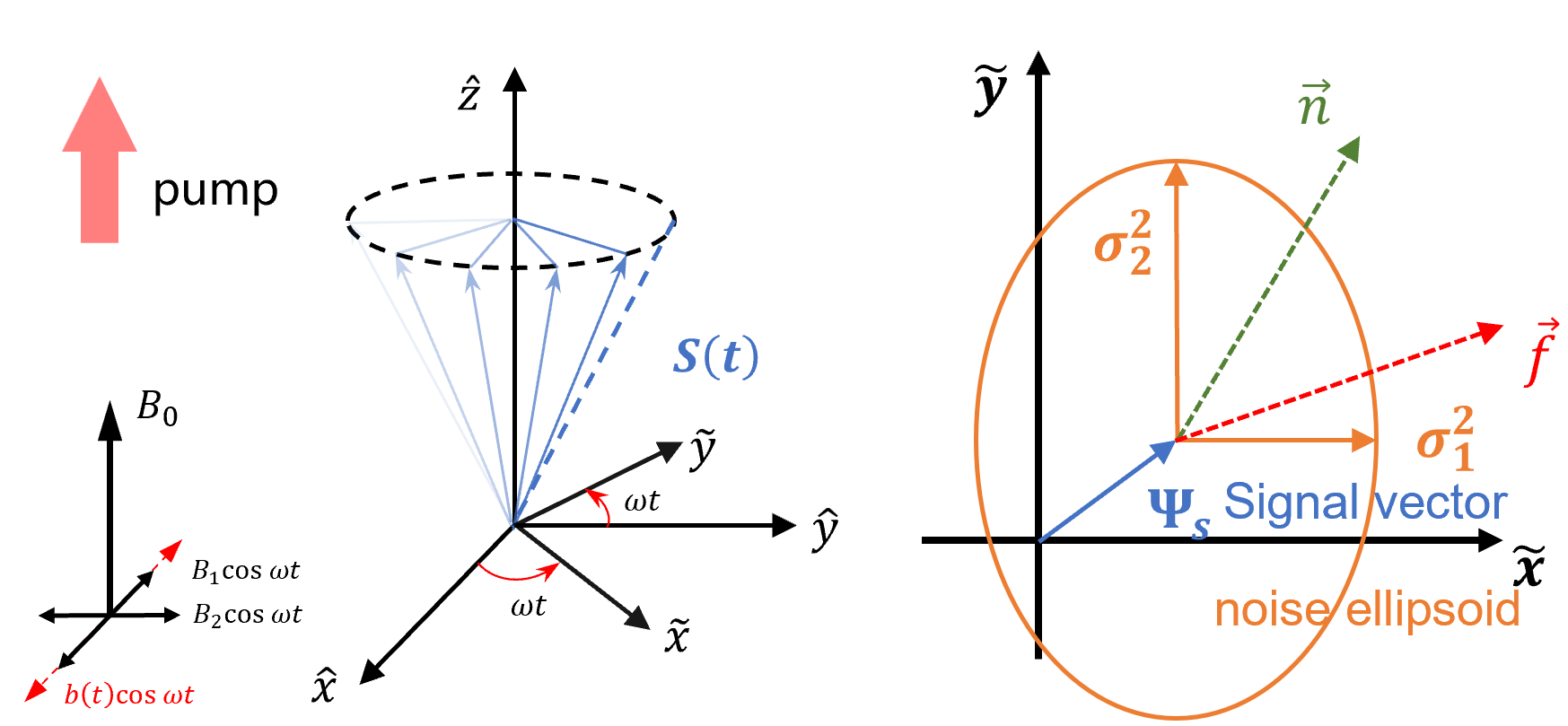
Equation (4) shows that the optimal fingerprint is, in general, unparalleled with the signal . The optimal detection direction is neither along the direction of the maximum of the signal nor the minimum of the noise (see Fig. 1).

| Climate System Hasselmann (1993, 1979) | Spin Resonance System | |
| dynamics |
climate models,
e.g., Global Climate Models |
Bloch equation |
| external forcing |
human and natural activities,
e.g., emissions of greenhouse gases from human activities |
magnetic field,
e.g, , |
| signal |
climate variables,
e.g., global mean surface temperatures |
atomic spin |
| noise | natural internal variability | spin noise induced by the magnetic field noise |
Fingerprint in spin system. - We simulate the complex climate system and examine the optimal fingerprint method by a well-controlled magnetic resonance system of spins. The spins now represent the climate system, while the magnetic field represents the external forcing in climate problems The model used to determine such response is the Bloch equation Bloch (1946); Happer (1972)
| (5) |
where is the spin vector, is the gyromagnetic ratio, is the magnetic field, and is the relaxation tensor with and being the longitudinal and transverse relaxation rate respectivelyAppelt et al. (1998); Franzen (1959). The magnetic field consists of a static field along the direction, which defines the Larmor frequency of the spins, and time-dependent fields and along and directions, which drive the precession of the spins. To be specific, we consider the following form of the transverse driving field
| (6) | |||||
| (7) |
The amplitude of is also modulated by a Gaussian white noise to simulate the natural noise. The correlation function of is , where characterizes the power spectrum density, and is a Dirac- like function with short correlation time .
In the weak driving limit, i.e., , and , the could be treated as a constant, so the observed signal should be a two-dimensional vector consisting of transverse components of the spin, namely,
| (8) |
where and denote the corresponding components in the rotating frame, and is the spin component in the laboratory frame.
It is worth mentioning that weak driving condition also guarantees the prerequisite of the optimal fingerprint method, namely, the expected signal driven by the external forcing, i.e. and , can be separated from the noise signal driven by .

In the resonant case, one obtains the expected signal and the covariance matrix of as
| (9) |
| (10) |
According to Eqs. (4) & (10), the optimal detection direction depends on the driving field amplitudes and as
| (11) |
which indicates the optimal fingerprint detection in the spin system.
The spin magnetic resonance system described by Eqs. (5)-(10) supports a fully controllable physical model to experimentally study the optimal fingerprint method. Various parameters in the spin system, including the relaxation rates and , the noise intensity , and the driving field amplitudes and , are tunable in a wide range to mimic the climate system. Furthermore, the resonance system contains several time scales, including (i) the correlation time of the noise is the shortest timescale in the system; (ii) the spin precession period ; (iii) the spin relaxation time and Seltzer (2008); Happer (1972); Appelt et al. (1998); Franzen (1959); and (iv) the characteristic timescale of the change of the driving field , which changes vary slowly and is the longest timescale in the system. The hierarchy of different time scales (i.e. ) mimics the complex dynamic behavior of climate system. Consequently, the spin resonance model is a suitable physical system for verifying fingerprint method.

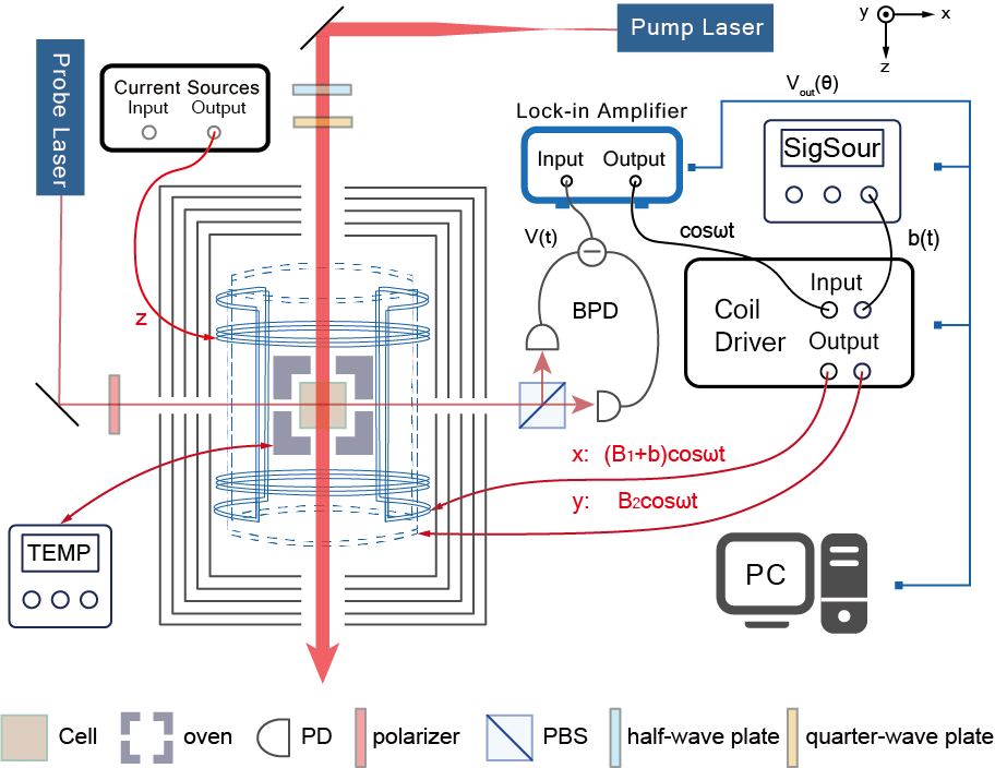
Experimental verification of fingerprint method. - The experiment setup is illustrated in Fig. (2). A glass cell filled with purified atoms and 350 Torr as buffer gas is placed in an oven, which is heated to . The atomic density of the Rb vapor at this temperature is . The glass vapor cell, the oven and a set of three-axis magnetic field coils are placed in a five-layer magnetic shield to eliminate the earth magnetic field and the unwanted magnetic noise. The Rb atomic spins are optically pumped by a circular polarized laser beam propagating along the direction in resonance with the D1 line of the Rb transition. The transverse spin component of Rb atoms in lab coordinates is detected by a linearly polarized laser beam along direction via the Faraday rotation effect Seltzer (2008). A magnetic field is applied along direction, corresponding to the Larmor frequency of spins. The deterministic amplitudes and of the driving field components are generated by the LIA, and the Gaussian noise is generated by a signal source. These signals are converted to the driving magnetic fields by the coil driver (see Fig. 2).
Experimentally, the signal is obtained directly by demodulating the voltage from the balance power detector (i.e. BPD, see Fig. 2) with a reference signal via a lock-in amplifier (LIA) , where is the demodulation phase Meade (1983). Given the phase , the demodulation output
| (12) |
is equivalent to a projection of the signal vector along the direction in the rotating frame. The fingerprint method is examined by measuring the SNR of the output of the spin system as a function of . The optimal fingerprint in Eq. (4) is indeed the projection direction which maximizes the SNR.

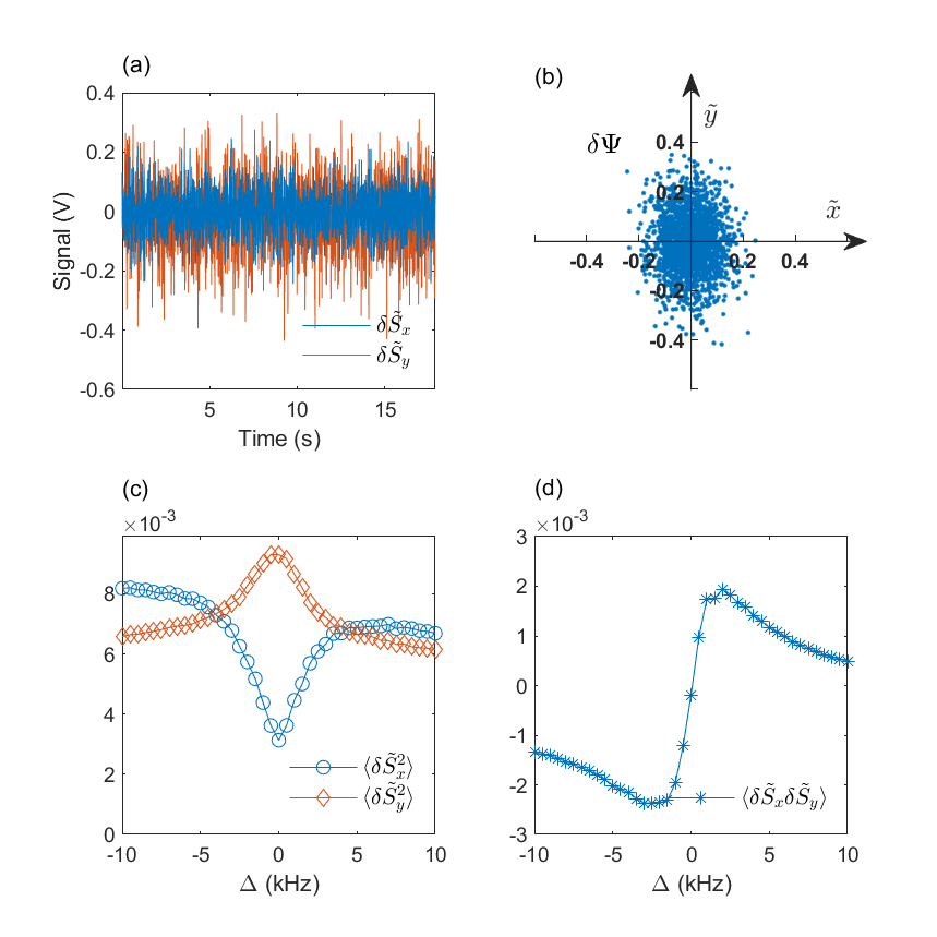
Figure 3 shows the measured spin signal vector and its statistical properties under the driving fields and in Eqs. (6) & (7). In the case of resonant driving (), with the demodulation phase or , the fluctuation of and induced by the noise field is obtained, as shown in Fig. 3(a). In the two-dimensional plane spanned by and , the distribution of the spin signal vector forms an ellipsoid with an aspect ratio of [see Fig. 3(b)], which agrees with the theoretical prediction of Eq. (10). The full covariance matrix of the spin fluctuation and its frequency dependence is also measured by varying the driving frequency . The variance of () shows a Lorentzian (anti-Lorentzian) lineshape, and the correlation function is of dispersive profile [Figs. 3(c) & (d)].
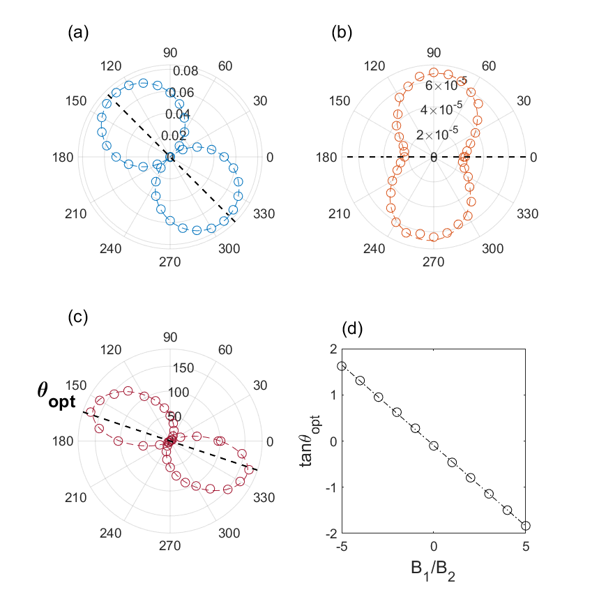
Measuring the signal along the or axes is not the optimal choice to extract the signal from the noise. Although the variance of the signal is small, the signal amplitude along the axis is also small. By setting the demodulation phase , we choose a measurement direction , along which the signal amplitude is a linear combination of and
| (13) |
and the variance is
| (14) |
To find the maximum SNR, we record the signal amplitude and the variance simultaneously while sweeping the measurement direction . As shown in Figs. 4(a) & 4(b), both signal amplitude and variance have their own maximum and minimum values, but they do not coincide in the same direction . According to the fingerprint method, there exists an optimal detection direction which maximizes the SNR. Figure. 4(c) shows the SNR as a function of the detection angle , and the optimal detection direction is indicated by the black dashed line.
Figure 4(d) shows the measured the optimal detection direction as a function of the ratio , and the dashed line indicates the theoretical prediction according to Eq.(11). The linear dependence between experiment data and theory agrees well indicating that the fingerprint method in the spin resonance system has been verified.
Conclusion.- In summary, we have experimentally verified the optimal fingerprint method faced on spin system. The spin system is a well-controlled physical model to mimic the complex climate system, and the optimal fingerprint method is examined by measuring the SNR of the output of the spin system as a function of the detection direction. The optimal detection direction is determined by the driving field amplitudes and , and the measured agrees well with the theoretical prediction. The experimental verification of the optimal fingerprint method in the spin system provides a solid foundation for the application of the optimal fingerprint method in the climate system. Furthermore, the verification makes fingerprint methods becoming a universal and conventional method in solving attribution problems faced on other physical system.
References
- WMO; ICSU;International Study Conference (1975) (29 July - 10 August 1974) WMO; ICSU;International Study Conference (29 July - 10 August 1974), The Physical Basis of Climate and Climate Modelling: Report of the International Study Conference in Stockholm, 29 July-10 August 1974, 16 (World Meteorological Organization, 1975).
- Hansen et al. (1983) J. Hansen, G. Russell, D. Rind, P. Stone, A. Lacis, S. Lebedeff, R. Ruedy, and L. Travis, Monthly Weather Review 111, 609 (1983).
- Weart (2010) S. Weart, Studies in History and Philosophy of Science Part B: Studies in History and Philosophy of Modern Physics 41, 208 (2010).
- Manabe and Wetherald (1975) S. Manabe and R. T. Wetherald, Journal of Atmospheric Sciences 32, 3 (1975).
- Voldoire et al. (2013) A. Voldoire, E. Sanchez-Gomez, and D. Salas y Mélia.et al., Climate Dynamics 40, 2091 (2013).
- Hasselmann (1976) K. Hasselmann, Tellus A 28, 473 (1976).
- Frankignoul and Hasselmann (1977) C. Frankignoul and K. Hasselmann, Tellus 29, 289 (1977).
- Lemke (1977) P. Lemke, Tellus 29, 385 (1977).
- Hasselmann (1993) K. Hasselmann, Journal of Climate 6, 1957 (1993).
- Hasselmann (1979) K. Hasselmann, Meteorology over the tropical oceans , 251 (1979).
- Hasselmann (1997) K. Hasselmann, Climate Dynamics 13, 601 (1997).
- Allen and Tett (1999) M. R. Allen and S. F. B. Tett, Climate Dynamics 15, 419 (1999).
- Ribes et al. (2013) A. Ribes, S. Planton, and L. Terray, Climate Dynamics 41, 2817 (2013).
- Hegerl and North (1997) G. C. Hegerl and G. R. North, Journal of Climate 10, 1125 (1997).
- Hegerl et al. (1996) G. C. Hegerl, H. von Storch, K. Hasselmann, B. D. Santer, U. Cubasch, and P. D. Jones, Journal of Climate 9, 2281 (1996).
- Hegerl et al. (1997) G. C. Hegerl, K. Hasselmann, U. Cubasch, J. F. B. Mitchell, E. Roeckner, R. Voss, and J. Waszkewitz, Climate Dynamics 13, 613 (1997).
- Stott et al. (2003) P. A. Stott, M. R. Allen, and G. S. Jones, Climate Dynamics 21, 493 (2003).
- Sun et al. (2014) Y. Sun, X. Zhang, F. W. Zwiers, L. Song, H. Wan, T. Hu, H. Yin, and G. Ren, Nature Climate Change 4, 1082 (2014).
- Santer et al. (2019) B. D. Santer, C. J. W. Bonfils, Q. Fu, J. C. Fyfe, G. C. Hegerl, C. Mears, J. F. Painter, S. Po-Chedley, F. J. Wentz, M. D. Zelinka, and C.-Z. Zou, Nature Climate Change 9, 180 (2019).
- Masson-Delmotte et al. (2021) V. Masson-Delmotte, P. Zhai, S. Pirani, C. Connors, S. Péan, N. Berger, Y. Caud, L. Chen, M. Goldfarb, and P. M. Scheel Monteiro, Ipcc (2021).
- Bloch (1946) F. Bloch, Phys. Rev. 70, 460 (1946).
- Happer (1972) W. Happer, Rev. Mod. Phys. 44, 169 (1972).
- Appelt et al. (1998) S. Appelt, A. B.-A. Baranga, C. J. Erickson, M. V. Romalis, A. R. Young, and W. Happer, Phys. Rev. A 58, 1412 (1998).
- Franzen (1959) W. Franzen, Physical Review 115, 850 (1959).
- Seltzer (2008) S. J. Seltzer, Developments in alkali -metal atomic magnetometry, Ph.D. thesis, Princeton University (2008).
- Meade (1983) M. L. Meade, Lock-in amplifiers : principles and applications (Institution of Electrical Engineers, 1983).