Stein Variational Ergodic Search
Abstract
Exploration requires that robots reason about numerous ways to cover a space in response to dynamically changing conditions. However, in continuous domains there are potentially infinitely many options for robots to explore which can prove computationally challenging. How then should a robot efficiently optimize and choose exploration strategies to adopt? In this work, we explore this question through the use of variational inference to efficiently solve for distributions of coverage trajectories. Our approach leverages ergodic search methods to optimize coverage trajectories in continuous time and space. In order to reason about distributions of trajectories, we formulate ergodic search as a probabilistic inference problem. We propose to leverage Stein variational methods to approximate a posterior distribution over ergodic trajectories through parallel computation. As a result, it becomes possible to efficiently optimize distributions of feasible coverage trajectories for which robots can adapt exploration. We demonstrate that the proposed Stein variational ergodic search approach facilitates efficient identification of multiple coverage strategies and show online adaptation in a model-predictive control formulation. Simulated and physical experiments demonstrate adaptability and diversity in exploration strategies online.
I Introduction
Effective robotic exploration requires robots to reason about different ways to explore a space. In the presence of uncertainty and in unstructured environments, having multiple exploration strategies for robots to quickly choose from can be advantageous. However, optimizing for multiple exploratory paths can be computationally challenging, especially in continuous domains where trajectory solutions are infinite dimensional. Defining the problem of exploration on a grid [11, 5, 14, 37] can provide the means to enumerate many coverage paths; however, grid-based methods limit where the robot can visit in continuous, unstructured environments.
Recent advancements in curiosity- and information- based exploration have allowed robots to explore vast domains [37, 27, 24, 34, 9]. However, they are often limited to exploring using one strategy, i.e., an information maximizing strategy. As a result, exploring becomes myopic where immediate information gain is sought after without regard to advantageous states in the future. Ergodicity-based exploration techniques show promise in breaking away from myopic strategies by posing exploration as a coverage problem based on time-averaged trajectory visitation [23, 25]. More specifically, ergodic methods optimize over where trajectories spend time on average as a function of the expected measure of information. As a result, ergodic search methods allow robots to optimize exploratory paths in multi-modal search problems [26]. While the literature has proven ergodic-methods to produce effective exploration strategies, they only optimize one search strategy at any given moment, thus limiting how robots can adapt.

Prior work suggests that the non-convex form of ergodic search methods are capable of identifying multiple optimal trajectories through variations in initial condition [25]. The challenge with reasoning about multiple, i.e., distributions, of trajectories is that the optimization can become computationally prohibitive. Furthermore, there is no guarantee that certain initial conditions will not converge onto the same ergodic search strategy which is not ideal, especially in online exploration scenarios where mode collapse on trajectory solutions can have catastrophic consequences.
Stein variational inference methods show promise in providing the necessary tools to approximate distributions of trajectories in a computationally tractable manner [22]. These methods leverage approximate inference in a non-parametric manner that 1) empirically estimates complex distributions, and 2) can do so in a computationally efficient manner through parallel computation. Thus, in this work, we propose a novel formulation of ergodic exploration using Stein variational gradient decent methods [22] that solves an inference problem on distributions of trajectories. We find that the spectral construction of the ergodic metric promotes discovery of locally optimal solutions which can be leveraged to guide robot exploration with multiple redundancies. We demonstrate the efficacy of our approach in simulation and on a physical drone system that can efficiently and effectively adapt exploration in cluttered environments. Furthermore, we find that the synergy between Stein variational methods and ergodic search methods promotes a diverse range of exploration strategies which can be acquired in a computationally efficient manner. In summary, our contributions are
-
1.
A Stein variational ergodic search method for trajectory optimization and control;
-
2.
Demonstration of diverse exploration strategies in a computationally efficient manner; and
-
3.
Real-time exploration and adaptation of multiple ergodic trajectories in dynamic domains.
The remainder of the paper is structured as follows: Section §II provides an overview of related work, Section §III-A introduces the problem of coverage via ergodic search, Section §III-B introduces the Stein variational gradient descent, Section §IV derives the proposed Stein variational ergodic search approach, and Sections §V, and §VII presents the results and conclusions.
II Related Work
Coverage and Exploration. Robotic exploration seeks to guide robots towards unexplored areas within a domain. Likewise, coverage is concerned with generating paths and placement of a robot’s sensors such that it covers a bounded domain [8, 3]. Early solutions to coverage and exploration are often formulated over discrete grids (defined on continuous space) and shown to have completeness guarantees through novel boustrophedon search patterns (which originates the lawnmower pattern [11]) and the traveling salesperson problem [4, 19]. Through grids, it is relatively straightforward to use exhaustive computational techniques to enumerate the many different, feasible paths a robot can take to explore and cover an area. Extending these ideas to continuous domains (which provides infinite spatial resolution for the robot to traverse) often proves challenging as the number of possible ways to explore a domain becomes infinite.
Recent methods in reinforcement learning and information-based methods circumvent the issues with transitioning to continuous domains by leveraging “curiosity” measures [27, 7] derived from information theory [10] to encourage exploration. These measures provide a signal which informs a robot where it is beneficial to visit and have demonstrated comparability with continuous domains [27, 24]. However, many of these methods tend to be myopic in nature, only focusing on immediate information gain, and often limited to single-mode solutions which can limit the adaptability of robots in the wild. More recent efforts in ergodicity-based methods (also referred to as ergodic exploration, coverage, or search) have demonstrated that it is possible to compute intricate coverage patterns through a spectral-based metric over continuous domains [26, 1, 12]. Ergodicity-based methods generate coverage by minimizing the difference between the (expected) spatial distribution of information and the time-averaged spatial distribution of an agent’s trajectory within the domain [23]. Interestingly, prior work has provided evidence that suggests ergodic coverage strategies produce optimal exploration strategies [13]. The spectral, multi-scale composition of the ergodic metric [31] suggests there exist many solutions that can be exploited by robots. However, it has yet to be demonstrated how one can calculate sets of “good”, locally-optimal ergodic trajectory solutions that a robot can adapt as its search strategy.
Control as Inference. The introduction of probabilistic inference to optimal control has enhanced the capabilities of robots via sample-based methods. Specifically, the non-convexity of many robot task specifications makes it challenging for gradient-based methods to find reasonable trajectory solutions that satisfy a task. Incidentally, this is caused by the non-convexity of many robotic tasks due to its specification or the underlying complexity of the interactions, e.g., contact dynamics. Sample-based methods derived from probabilistic inference circumvent these issues through zero-order optimization, e.g., predictive sampling [15], and model-predictive path integral (MPPI) [39, 38], that are less sensitive to the non-convexity of robotic tasks. Add in the significant technological leap of GPU-based computation, and control as an inference problem becomes a powerful tool for robotics. However, like with gradient-based methods, many of the sample-based techniques typically solve for only one locally optimal solution, ignoring other equally viable ways to solve a task.
Having more than one plan for which robots can switch between is highly valuable for real-world systems that need to quickly change strategy. For example, in crowd-based navigation, certain planned paths often become infeasible due to the dynamically changing environment. Rather than having to recalculate a new path, it is more efficient and robust for a robot to have several paths to choose from [35, 18]. The recent adoption of optimal transport and variational methods in optimal control has demonstrated promise is isolating the many locally optimal solutions for robots to choose from [20, 18]. These approaches pose trajectory solutions to non-convex optimal control problems as inference problems were solutions are approximated as distributions. As a result, it becomes possible for robots to optimize for many locally optimal solutions and adapt in real-time. However, most of the applications have focused on obstacle avoidance and point-to-point navigation. Exploration and coverage has not yet been explored primarily due to 1) the difficulty of forming coverage objectives in continuous domains, and 2) stable convergence of solutions over long-time horizons.
In this work, we demonstrate it is possible to solve for many coverage trajectory solutions in continuous space that promote diverse and robust exploration over long-time horizons by forming ergodic coverage methods as an inference problem and leverage second-order Stein variational gradients [18, 22] to converge on solutions.
III Background and Preliminaries
III-A Ergodic Search
Let us first define a robot’s state space and control space as and . Next let us define the robot’s state trajectory as the solution to the initial value problem
| (1) |
where is an initial condition, is a control trajectory, and is the continuous-time (potentially nonlinear) dynamics of the robot. We denote
| (2) |
as the set of all continuous trajectories defined on arbitrary finite time intervals. In addition, let us define a bounded domain where the robot explores as , where and are the bounds of the workspace. We fix a map that projects state space to exploration space , e.g., a selection matrix that isolates and scales certain states that correspond to exploration.
Definition 1.
Time-Averaged Trajectory Statistics. Let denote the Lebesgue measure on , be a trajectory, and . For each , let the probability measure on that defines the time-averaged trajectory visitation statistics integrated along time be defined by
| (3) |
where is a Borel set.
Definition 2.
Ergodicity. A trajectory is ergodic with respect to a Borel probability measure on if converges weakly to as . That is,
| (4) |
for all continuous functions . In particular, the trajectory statistics measure can be viewed as an integral of delta functions, where
| (5) |
Roughly speaking, a trajectory is ergodic with respect to the measure if it eventually (as ) explores the workspace in a manner which is commensurate with . This is formalized by requiring the measure , which quantifies the proportion of time the trajectory is contained in subsets during the interval , to converge to . Because is compact, weak convergence is defined by
| (6) |
for all integrable functions . However, since robots only run for finite time horizons, we must quantify the level of ergodicity of finite trajectories.
Definition 3.
Ergodic Cost Function. Let be a probability measure on . A -ergodic cost function is a function such that for an infinite trajectory , if as then is ergodic.
To define the ergodic metric for trajectory optimization, we use spectral methods and construct a metric in the Fourier space [23, 31, 26].
Definition 4.
Spectral Ergodic Cost Function. Let be a probability measure on . Let be the set of all integer fundamental frequencies that define the cosine Fourier basis function
| (7) |
where is a normalizing factor (see [26, 23]). For a finite trajectory , let be the measure defined in Eq. (3). The spectral ergodic cost function is defined as
| (8) | ||||
where and are the Fourier decomposition modes of and , respectively (using Eq. (5)), and is a weight coefficient that places higher importance on lower-frequency modes.
In particular, the spectral ergodic cost function defined for a probability measure forms a metric [23] which is able to generate coverage trajectories at arbitrary spacial scales [31] (which we additionally prove in Appendix A-A). This is advantageous as 1) the metric defines a proper coverage distances using spectral modes in continuous space; and 2) specifies infinitely many ways to explore with respect to the spectral decomposition. Note that while the ergodic metric forms a non-convex objective in the trajectory space, the non-convexity specifies many trajectory solutions that robots can take leverage to improve exploration. The challenge is then optimizing for the distribution of feasible ergodic trajectory solutions.
We can formulate an optimization problem over trajectories through the ergodic metric. Consider that is constrained (either through dynamics (1) or through some other differential constraints). Then the ergodic trajectory optimization is given as
| (9) | ||||
| subject to | ||||
where initial conditions and input trajectory constraints can be accounted for in the equality and inequality constraints , e.g., and .
III-B Stein Variational Gradient Descent
A powerful method to perform probabilistic inference is variational inference (VI), where one aims to approximate a complex target distribution with a candidate distribution from a parameterized family of distributions . This is typically achieved by minimizing the Kullback-Leibler (KL) divergence,
| (10) |
However, finding an appropriate family which balances accuracy with tractable computations is often challenging. Stein variational gradient descent (SVGD) [22] addresses this issue by providing a nonparametric method to sample from the target distribution via kernel methods and gradient descent.
The Stein variational method is derived by sampling a collection of points using a prior distribution on , and then iteratively updating them by the gradient descent
| (11) |
In particular, is the step size, and is the vector field which maximally decreases the KL-divergence at the step (not to be confused with fundamental frequency).
Suppose is a positive definite kernel, and is its corresponding reproducing kernel Hilbert space (RKHS). We restrict the vector field to be the function class , and therefore
| (12) |
where denotes the empirical distribution at step . Note that if the kernel is universal, is dense in the space of continuous functions , and does not result in a loss of generality. Furthermore, from [22], we have an exact form for ,
| (13) |
which can be approximated by samples
| (14) |
Thus, the sampled points converge onto an approximation of the distribution . In this work, we leverage the Stein variational gradients to define and solve for distributions of ergodic trajectories for robot exploration.
IV Ergodic Coverage as Inference
In this section, we pose the problem of computing ergodic trajectories as an inference problem over a distribution of paths. We then derive an algorithm for optimizing approximate distributions on ergodic paths and prove optimality of the posterior distribution of paths in the ergodic coverage inference problem.
IV-A The likelihood of ergodicity and Stein variations
In order to explore the landscape of trajectories which minimize an ergodic cost function, we will formulate the ergodic search problem in terms of variational inference. Adapting [18], which formulated motion planning problems using variational inference, we introduce a binary optimality criterion . Suppose is a probability measure on . Then let use this optimality to encode a -ergodic cost likelihood function by defining
| (15) |
where is a hyperparameter and we simplify the notation by using to denote the optimal condition . Given a prior distribution on , and a positive definite kernel on path space, we can use SVGD to sample from the posterior distribution . In particular, by applying Bayes’ rule, the optimal vector field from Eq. (13) for a -ergodic cost likelihood function is given by
| (16) |
where and is a prior over trajectories. The main benefit of forming an ergodic trajectory optimization through Stein variational descent is the ability to optimize multiple trajectories in parallel.
IV-B Ergodic Stein variational trajectory optimization
Instead of defining a distribution of infinite-dimensional trajectories, we discretize the path to facilitate numerical optimization. Let , where , be a collection of points representing a trajectory along a discrete time horizon indexed by discrete time (which we purposefully overload the notation to keep consistent with the stated definitions). Note that the definition of paths in Eq. (2), ergodicity in Def. 1, and as a cost function Def. 4 are now calculated on discrete paths and still hold. Next, let us define an empirical distribution over discrete paths as . Following Eq. (14), we approximate using where we assign where , and is the variance. Given a kernel function on discrete paths , the ergodic Stein variational step is given by
| (17) |
where minimizes the ergodic cost over the trajectory sample, and is a repulsive force that pushes trajectory solutions. We can view the kernel as a similarity measure between two trajectories . Specifically, as so does and as , (when choosing a radial basis kernel (24)). Thus, one can measure diversity of a set of particles using a kernel by forming a matrix with entries , (where ) and computing the determinant of we can establish a measure of diversity. In particular, given a set of trajectories , as and as .
Constraints on the trajectory and additional terms that shape trajectory solutions can be added by extending the cost likelihood function in the following form
| (18) |
where are positive penalty weights111 are chosen arbitrarily, but can be treated as Lagrange multipliers in an Augmented Lagrange formulation. that form an inner product with equality and inequality functions , and is any additional penalty terms on the trajectory . We can rewrite the ergodic Stein variational step using as
| (19) |
Selection of trajectories can be done through a heuristic operation
| (20) |
In Alg. 1 we outline the Stein variational ergodic trajectory optimization algorithm.
IV-C Ergodic Stein variational control
The ergodic Stein step Eq. (19) acts on discrete points that represent robot trajectories. We can readily extend this formulation over discrete control inputs . Consider the discrete-time transition dynamics
| (21) |
then, given an initial condition , and a sequence of controls , is calculated through recursive application of Eq. (21) starting from . Using this formulation, we can define the problem over control inputs where we optimize over and by an approximate distribution over control sequences . We can then optimize strictly over controls by using a kernel on discrete control paths , where the Stein variational step is
| (22) |
where is the ergodic metric of trajectory given initial condition and control sequence . This form is useful in adaptive model-predictive control (MPC) where direct control values are replanned online. As with trajectory optimization, we can rewrite the Stein step using Eq. (18) and introduce constraints on the control and trajectory as needed. In most MPC formulations, after the control trajectory is optimized, it is common to pass to the robot the first control value and shift the sequence of controls, i.e., to warm start the optimization. We follow [22] for updating the controls. We outline the Stein variational ergodic control in Alg. 2.
IV-D Kernel design for Ergodic trajectories
Exploration requires reasoning about long time horizons to promote effective coverage. This poses a problem as Stein variational methods tend to perform poorly in high-dimensional problems, e.g., for results in dimensional inference problem [40]. The repulsive terms that provide the diversity in solutions vanishes at higher dimensions (due to the derivative of the kernel diminishing with respect to its input). The most common way to effectively deal with the computational issues is by choosing a kernel of the form
| (23) |
where is a graph of connected points separated by time and is a sum of positive semi-definite kernels that leverages the Markov property of state trajectories [18] which we refer to as a Markov Kernel. As with prior work, a good choice of kernel is the smooth radial basis function (RBF)
| (24) |
where is a heuristic that takes the median of the particles. It is possible to choose the kernel to be a composition, e.g., a Markov RBF kernel, which we evaluate the effect of kernels on trajectory diversity in Section §V.
In this work, we leverage the multiscale aspect of ergodicity and the spectral ergodic metric and define the kernel and trajectories in the workspace where can be arbitrarily chosen to satisfy numerical conditioning, e.g., , and . Given an invertible and linear map , we can rewrite the trajectories in terms of the composition which significantly improves numerical conditioning of the kernel without loss of generality. Note that if then the Stein variational ergodic optimization problem reduces to a parallel trajectory optimization over random samples . Other choices can provide better options, but in this work we only consider the smooth RBF and the Markov RBF kernel.
IV-E Convergence
The convergence of SVGD has been actively studied, primarily in the population limit with infinitely many samples [21, 16, 30]. A non-asymptotic analysis of convergence was carried out in [16], and finite sample bounds for propagation of chaos have also been considered [33]. We show in Appendix A-B that SVGD converges in the present setting of ergodic search by applying [16, Corollary 6].
Theorem 1 (Informal).
Given the assumptions in this section and in the infinite particle limit, SVGD converges, where the gradient update steps are bounded by
| (25) |
where is a smooth prior distribution and is a constant.
Proof.
See Appendix A-B for formal proof. ∎
Convergence of SVGD subject to an ergodic metric is beneficial towards guaranteeing trajectory solutions can be acquired. In the following section we provide analysis and empirical results for our proposed approach.
V Results
In this section, we provide analysis and validation of our proposed approach. Specifically, we are interested in addressing the following:
-
1.
How diverse are Stein variational ergodic trajectories?
-
2.
Do optimized trajectories yield similar ergodic losses?
-
3.
How does the choice of kernel effect solutions?
-
4.
Can the approach handle additional constraints?
-
5.
Can the proposed approach adapt exploration in a real-time control setting?
Additional information regarding parameters, kernels, assumptions, and implementation details are provided in Appendix B. Multimedia for the results can be found in the supplementary material.
V-A Convergence and Trajectory Diversity
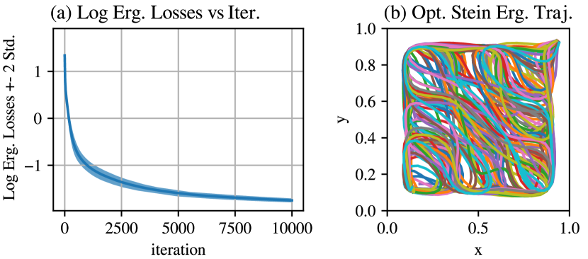
First, we are interested in evaluating whether the proposed Stein variational ergodic trajectory optimization method converges and provides diverse trajectories. In particular, we are interested in empirically evaluating how ergodic trajectories can be under a Stein variational approach. We consider the case of Alg. 1 in a 2-D planar uniform coverage problem in a bounded domain (see Fig. 2).
The trajectories are constrained such that each consecutive time step is regularized (ensuring smoothness of the paths). In addition, we bound the trajectories within the domain through a barrier function (see Appendix B). We evaluate a discrete sample of trajectories of length (initialized with a mean trajectory interpolating from some initial point to a final point on with additive zero mean Gaussian noise with variance . We set , i.e., a uniform distribution, to specify the ergodic metric.
Stein Ergodic Trajectory Convergence. As demonstrated in Fig. 2, the proposed Stein variational ergodic trajectory optimization converges each of the trajectories towards a minimum ergodic loss (shown in log form). Interestingly, the standard deviation of the ergodic losses for the trajectory remains significantly minimal (where we show standard deviation in Fig. 2). Visual inspection of the trajectories in Fig. 2 demonstrates the diversity in the optimized solutions which produce uniform coverage over the domain. This result emphasizes that synergy between the spectral ergodic metric and the Stein variational gradient descent, offering the effectiveness of non-parametric optimization in approximating a posterior over trajectories, and the ergodic metric producing complex trajectories that facilitates discovery of many exploration strategies.
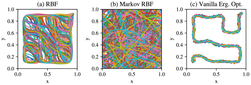
Stein Kernel Effect on Ergodic Trajectories. Analyzing the kernel gives us more insight as to its effect on producing diverse trajectories. In Fig. 4, we evaluate the proposed approach in Alg. 1 on three kernels, the RBF kernel (24), the Markov RBF [18] (23), and a kernel that reduces the Stein variational gradient to independent parallel gradient descent on a set of trajectories, i.e., a benchmark on the canonical vanilla ergodic trajectory optimization. We configure the problem as we did in the convergence analysis presented in Fig. 2 where is a uniform distribution and the trajectories (totalling ) are regularized to be Markovian. Each kernel is optimized until convergence of the ergodic metric (based on the gradient condition as described in Alg. 1). We find that the Markov RBF kernel produced significantly more diverse trajectories than the RBF kernel alone. This is expected as the Markov RBF kernel repels pair-wise trajectory points where RBF produces compares whole trajectories (which results in more regular trajectories). Compared to the base vanilla ergodic trajectory optimization, the proposed Stein variational ergodic approach significantly outperforms the benchmark, generating a diverse set of ergodic trajectories. Under the same initial conditions, the benchmark ergodic trajectory optimization produces the same ergodic trajectory, resulting in mode-collapse over the posterior and further supporting the need for the proposed Stein variational ergodic method.
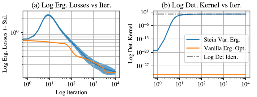
Stein Ergodic Trajectory Diversity. We can see the diversity of the trajectories more clearly in Fig. 3 where we compare the Stein variational ergodic approach with the vanilla ergodic metric. The kernel is given by Eq. (24) with . As seen in in Fig. 3, both methods converge towards an ergodic trajectory local minima. The Stein variational approach produces a wider range of local minima (based on standard deviation) and initially produces worse ergodicity (due to the trajectory diversification). The initial bump in the Stein variational ergodic losses are due to the initial trajectory diversification, as shown in Fig. 3 (b). The diversity measure is calculated using the determinant of the kernel matrix which converges on a diverse set of trajectories . Interestingly, this behavior does not influence the rate of change in the ergodic loss as both the Stein variational ergodic approach and the vanilla ergodic trajectory optimization converge onto the same levels of ergodicity within the same number of iterations. The trajectories calculated from parallel ergodic trajectory optimizations (without the repulsive force) collapses onto a single local minima which results in and non-unique trajectory solutions.
V-B Large-Scale and Constrained Exploration
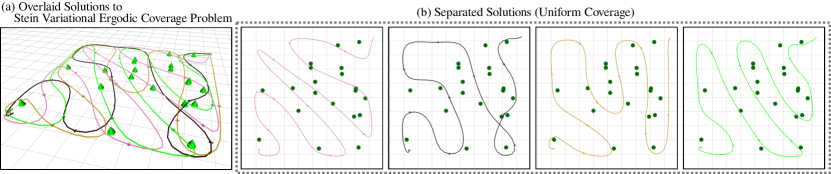
Next, we consider real-world problem scenarios where exploration occurs in a constrained environment (with obstacles and dynamic constraints). Our first examples looks at generating diverse exploratory trajectories in a simulated forest. The goal is to generate uniform coverage over a larger domain () and demonstrate the flexibility of the proposed approach when dealing with arbitrary scales, and introduce several obstacles representing trees. The trajectories are constrained to be Markovian (via a penalty term, see Appendix B) to match velocity constraints that are feasible for a drone to follow. The trajectories are solved over seconds to indicate the larger-scale aspect of the example, and are required to start and end at the same point (to further emphasize the diversity of solutions). The trees are represented as disk penalty terms that encompass the width of the tree (and is known at optimization time).
Multiscale Coverage in a Forest. As illustrated in Fig. 5 is an example of solutions to the Stein ergodic trajectory optimization in the cluttered forest environment. Note that the initial and final positions are same for each trajectory (due to the cost-terms, see Appendix B), and yet the proposed approach is capable of generating highly diverse solutions (with just trajectory samples). In addition, the computation of the trajectory incurred no additional cost as the function map was the only element that was altered (other than the cost terms). As a result, the trajectories were produced with relative ease owing to the synergy between the ergodic metric with Stein variational methods, especially in terms of problem scale.
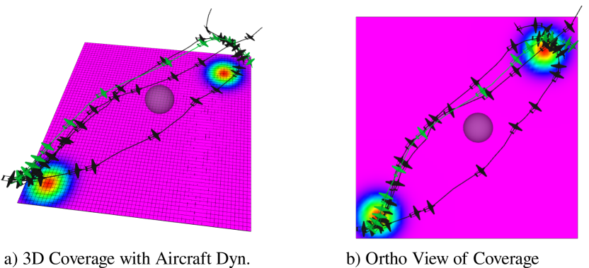
Diverse Coverage with Nonlinear Dynamics. We additionally evaluate our proposed method to generate diverse coverage with nonlinear robot dynamic constraints (see Fig. 6). The dynamics of the robot are given by a nonlinear aircraft model (see Appendix B). The trajectory length is given by with and the Markov RBF kernel (23) was used in this example. We use the Stein variational ergodic controller (Alg. 2) to produce a distribution of diverse exploratory trajectories that avoids the spherical obstacle in the middle. The generated trajectories leverage the nonlinear aircraft dynamics to go around the obstacle and avoid collision while slowing down around the bimodal peaks to generate coverage.
V-C Online Planning and Adaptive Exploration
Last, we explore the capability of the proposed approach for online planning and adaptive exploration through the use of the Stein variational ergodic model-predictive controller (Alg. 1). In particular, we are interested in leveraging the parallel nature of the proposed approach for exploration to efficiently compute exploration strategies in dynamic environments. We evaluate the proposed controller as a receding-horizon planner, which recomputes control strategies based on new information, in a exploration problem with dynamic obstacles. The obstacles are assumed to be observable after they move (and thus only their positions are known to the solver). We plan with a fixed time horizon of steps starting from the robot’s current initial condition and plan using trajectories with an RBF kernel. The dynamics are given by a single-integrator system with velocity limits that match the Crazyflie 2.1 drone [29]. The underlying information measure is given by a mixture of Gaussians placed asymmetrically over a bounded 2-D domain.
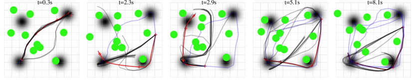
Online Planning and Control. In Fig. 7 we demonstrate the proposed receding-horizon Stein variational ergodic controller. Illustrated is a time-series snapshot of the controller producing several paths at various stages that avoids obstacles and provides alternative routes to explore the high-density areas. The selected path (in red) is based on the maximum of the cost likelihood model at the given planning time. As a result, it is typical that the approach switches between coverage strategies based on the immediate information obtained form observing the environment.
Interestingly, we find the proposed control approach is still able to reason about complex trajectories that visit multiple modal peaks within a single path. This is an exceptionally advantageous capability that provide within-trajectory diversity without resorting to heuristics or sample-based augmentations e.g., control randomness [39]. This can be seen through the smoothness of the planned trajectory paths (note in this example a trajectory smoothness penalty was not used as the underlying dynamic constraints naturally induce Markov trajectories). Furthermore the proposed approach visited each of the modal peaks within a run of the controller, even when the obstacles cluttered around one another and cut off certain paths. The proposed controller generates coverage trajectories around the free space proportional to the utility of information in that space. In this scenario, the trajectories will remain in the collision-free space until a path opens, leading to a fast traversal as the ergodic metric will penalize staying in the same area for too long.
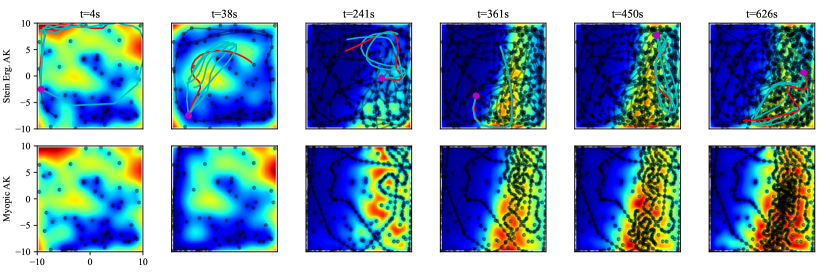
Sensor-based Exploration. We also demonstrate how our proposed approach can readily incorporate sensors and information measures to guide exploration. A sonar-based mapping problem as described in [9] is used to demonstrate this added capability. The goal is to map an environment using a sonar sensor (see [9] Fig. 7). We adopt the Attentive Kernel (AK) model where we compare against the myopic, sample-based planner that was used for finding where to sample data (as described in [9]). The information measure is defined as the entropy of the Attentive Kernel Gaussian process and is inserted into the Stein variational MPC as the utility measure . A total of samples are used to compute the Fourier transform of numerically based on the attentive kernel model (as done with the myopic planner). The same experiment settings are maintained where we choose sample locations based on the exploration path determined by the Stein variational ergodic approach (with a budget of 700 data points). Standard Gaussian process metrics are used to compare the quality of the Gaussian process as a function of data like, standardized mean square error (SMSE), mean standardized log loss (MSLL), root-mean-square error (RMSE), mean negative log-likelihood (MNLL), and mean absolute error (MAE) as done in [9].
Empirical results for the resulting Gaussian process metrics are reported in Table I. The results are averaged over 5 runs of each algorithm subject to the same random seed. Note that the proposed Stein variational ergodic approach improves the each metric without explicit fine-tuning to the sensor. As demonstrated in Fig. 8, the proposed Stein variational ergodic approach generates several exploration plans that plan useful data acquisition across multiple high-information peaks. In contrast, the myopic planner sets goal points based on a single plan but does not consider the effect collecting the data may have on the overall information landscape. As a result, how data points are distributed is significantly different across methods as our proposed approach spreads out data proportional to the entropy measure rather than densely sampling in only high-entropy areas. It is worth noting that our approach is not specific to the exact sensor or how we define information. The only restriction is that we are able to at least sample from the information distribution to compute the Fourier transform.
| SMSE | MSLL | NLPD | RMSE | MAE | |
|---|---|---|---|---|---|
| Stein. Erg. | 0.0669 | -1.6556 | 4.0504 | 16.6373 | 11.6971 |
| Myopic Plan. | 0.0765 | -1.6498 | 4.1785 | 17.7783 | 12.2943 |
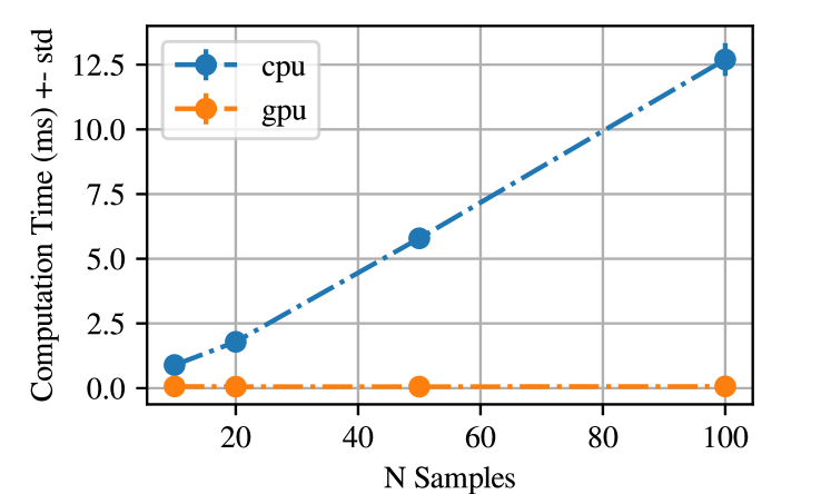
Computational Analysis. We additionally analyze the computational time of the proposed method. In Fig. 10, we find that CPU-based computation (using an AMD Threadripper 3960X) and acceleration through JAX [6] we get linear computational scaling with respect to the number of samples (holding the time horizon constant). With GPU-based computation and JAX (using an NVIDIA RTX 3080) we get constant scaling (with the worse computation time of . The increase in computation is as a result of the spectral nature of the ergodic metric. Specifically, one can additionally distribute the ergodic metric and gradient computation quite effectively which further improves the computation time, allowing for real-time control.
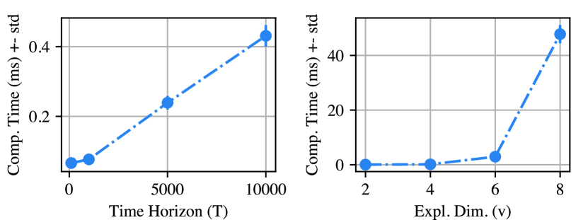
Furthermore, we provide a brief computational complexity analysis of our methods; in particular for one SVGD step described in Eq. (19), where we assume the paths are valued in an exploration space of dimension . This Stein variational step requires the computation of both the kernel matrix , which has a cost of , and the gradient , which requires the computation of gradients on an -dimensional space. We must also compute the spectral ergodic cost function, which is common to all ergodic search methods. For basis functions in each dimension, the ergodic cost function from Eq. (8) has a complexity of . We emphasize that all of these computations are parallelized in practice, and Fig. (11) demonstrates the effective parallelized scaling behavior.
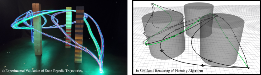
V-D Experimental Validation
We demonstrate empirical validation of the proposed Stein variational ergodic search method on a 3D uniform coverage problem in a crowded domain (see Fig. 12). We solve for a set of ergodic trajectories (using Alg. 1) at a length of with a time step . The coverage problem is defined over the 3D domain . Trajectories are constrained to satisfy feasible drone velocities according to the specifications of the Crazyflie 2.1 drone [29]. The best trajectory is selected based off the heuristic (20). The path was tracked using a low-level PID controller We find close correspondence with the planned trajectories and what the drone was able to execute in the in a physical experiment. Furthermore, the diversity in coverage solution can be used to readily adapt exploration as needed.
VI Limitations and Best Practises
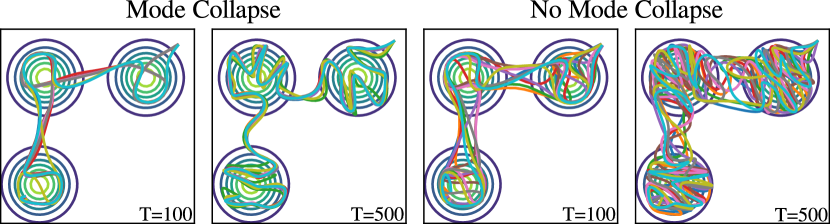
Mode Collapse. A well-known issue with SVGD is the reduction of the repulsive force in Eq. (19) as the dimensionality of the input space increases. This causes the particles to concentrate in the modes of the target distribution potentially diminishing its exploration capabilities and accuracy to capture long-tail distributions. Fortunately, there are several ways to deal with high dimensional inputs by exploiting the structure of our problem. In particular, since we are planning over the space of trajectories, there is an implicit Markovian assumption over the inference variables. This allow us to construct structured kernels such as the sum of kernels defined over subsets of variables that minimize the impact of performing inferences over long sequences [40]. We demonstrate an example of mode collapse in Fig. (9) by explicitly setting the repulsive force in Eq. (19) to zero.
Scaling. We demonstrate in Fig. (11) that the Stein variational gradient step empirically scales linearly in the time horizon due to the added parallelization, despite the complexity of the kernel matrix evaluation. However, we empirically observe quadratic scaling with respect to the scaling dimension due to the exponential number of basis functions required in the ergodic cost function (8). This scaling behavior is inherently a part of the definition of the spectral cost function and is independent to our primary contribution of incorporating SVGD into ergodic search. This is a well-known limitation in the literature [26, 31], and various methods to address this have recently been studied [2, 32, 36]. Our Stein methodology is already able to generate multiple diverse trajectories within these limitations, and we plan to address these scaling limitations in future work.
Best Practises. We found that the less nonlinear the constraints are the easier it was to produce ergodic trajectories. This is true in most trajectory optimization and model-predictive control approaches. However, certain aspects and choices have more influence as a result of the limitations discussed earlier. For example, longer time horizons can be optimized and yield non-myopic search strategies with the appropriate choice of time step for the dynamics. Similarly, one can achieve very poor and myopic search strategies when the step-size is chosen too small (which is highly dependent on the time-scale of the dynamics). Prior work on the impact of integration scheme and step-size has been explored [28] in isolation and should be referred to for best practises in choosing an appropriate time step and time horizon.
Another consideration is the number of basis functions used for computing the ergodic spectrum. The more features that the underlying information measure has, the more beneficial it is to have a high number of basis functions (see Fig. 8). This can incur additional computational costs, especially in high-dimensional exploration tasks. Specialized order reduction techniques, e.g., [32], can be used to effectively reduce the required number of basis functions and parallelization can further reduce computational overhead. A related consideration is the step-size of the stein variational gradient. We found that a step-size was sufficient for most problems and varied depending on the problem complexity and numerical scale, i.e., the more nonlinear the constraints and objective the smaller has to be to converge. A line search can be performed to find the optimal step-size for the specific problem.
VII Conclusion
In summary, we present a novel formulation of coverage and exploration as a variational inference problem on distributions of ergodic trajectories. Efficient computation of posterior ergodic trajectories was facilitated through Stein variational inference that provided sufficient parallelization and approximate inference to make the problem tractable. We found that the Stein variational gradients were well suited to being formulated with ergodic metrics as the natural multiscale aspect of ergodicity produces numerically well-behaved gradients for trajectory optimization and model-based control. As an outcome, we proposed two algorithms: 1) for directly computing distributions of ergodic trajectories; and 2) for calculating robust online model-predictive controller for robotic exploration.
We demonstrated empirical evidence that showed our proposed approach generated diverse trajectories that can be used for exploration and proved convergence of our approach to optimal ergodic trajectories. Constraints and multiscale implementations were demonstrated as an advantage of our approach through several simulated examples. Furthermore, we show the computational efficiency of our approach through parallel compute which was further improved by the spectral composition of computing ergodic trajectories. Physical experiments on a drone provided additional validation of our approach on real-world systems for robust and adaptive exploration.
Acknowledgments
DL was supported by the Hong Kong Innovation and Technology Commission (InnoHK Project CIMDA). CL, IA are supported by Yale University.
References
- Abraham et al. [2020] Ian Abraham, Ahalya Prabhakar, and Todd D Murphey. Active area coverage from equilibrium. In Algorithmic Foundations of Robotics XIII: Proceedings of the 13th Workshop on the Algorithmic Foundations of Robotics 13, pages 284–300. Springer, 2020.
- Abraham et al. [2021] Ian Abraham, Ahalya Prabhakar, and Todd D Murphey. An ergodic measure for active learning from equilibrium. IEEE Transactions on Automation Science and Engineering, 18(3):917–931, 2021.
- Acar et al. [2002] Ercan U Acar, Howie Choset, Alfred A Rizzi, Prasad N Atkar, and Douglas Hull. Morse decompositions for coverage tasks. The international journal of robotics research, 21(4):331–344, 2002.
- Applegate et al. [2011] David L Applegate, Robert E Bixby, Vašek Chvátal, and William J Cook. The traveling salesman problem. In The Traveling Salesman Problem. Princeton university press, 2011.
- Bähnemann et al. [2021] Rik Bähnemann, Nicholas Lawrance, Jen Jen Chung, Michael Pantic, Roland Siegwart, and Juan Nieto. Revisiting boustrophedon coverage path planning as a generalized traveling salesman problem. In Field and Service Robotics: Results of the 12th International Conference, pages 277–290. Springer, 2021.
- Bradbury et al. [2018] James Bradbury, Roy Frostig, Peter Hawkins, Matthew James Johnson, Chris Leary, Dougal Maclaurin, George Necula, Adam Paszke, Jake VanderPlas, Skye Wanderman-Milne, and Qiao Zhang. JAX: composable transformations of Python+NumPy programs, 2018. URL http://github.com/google/jax.
- Burda et al. [2018] Yuri Burda, Harri Edwards, Deepak Pathak, Amos Storkey, Trevor Darrell, and Alexei A Efros. Large-scale study of curiosity-driven learning. In International Conference on Learning Representations, 2018.
- Butler et al. [1999] Zack J Butler, Alfred A Rizzi, and Ralph L Hollis. Contact sensor-based coverage of rectilinear environments. In Proceedings of the 1999 IEEE international symposium on intelligent control intelligent systems and semiotics (Cat. No. 99CH37014), pages 266–271. IEEE, 1999.
- Chen et al. [2022] Weizhe Chen, Roni Khardon, and Lantao Liu. AK: Attentive Kernel for Information Gathering. In Proceedings of Robotics: Science and Systems, New York City, NY, USA, June 2022. doi: 10.15607/RSS.2022.XVIII.047.
- Chirikjian [2011] Gregory S Chirikjian. Stochastic models, information theory, and Lie groups, volume 2: Analytic methods and modern applications, volume 2. Springer Science & Business Media, 2011.
- Choset [2000] Howie Choset. Coverage of known spaces: The boustrophedon cellular decomposition. Autonomous Robots, 9:247–253, 2000.
- Dong et al. [2023] Dayi E Dong, Henry P Berger, and Ian Abraham. Time Optimal Ergodic Search. In Proceedings of Robotics: Science and Systems, Daegu, Republic of Korea, July 2023. doi: 10.15607/RSS.2023.XIX.082.
- Dressel and Kochenderfer [2018] Louis Dressel and Mykel J Kochenderfer. On the optimality of ergodic trajectories for information gathering tasks. In 2018 Annual American Control Conference (ACC), pages 1855–1861. IEEE, 2018.
- Galceran and Carreras [2013] Enric Galceran and Marc Carreras. A survey on coverage path planning for robotics. Robotics and Autonomous systems, 61(12):1258–1276, 2013.
- Howell et al. [2022] Taylor Howell, Nimrod Gileadi, Saran Tunyasuvunakool, Kevin Zakka, Tom Erez, and Yuval Tassa. Predictive sampling: Real-time behaviour synthesis with mujoco. arXiv preprint arXiv:2212.00541, 2022.
- Korba et al. [2020] Anna Korba, Adil Salim, Michael Arbel, Giulia Luise, and Arthur Gretton. A Non-Asymptotic Analysis for Stein Variational Gradient Descent. In Advances in Neural Information Processing Systems, volume 33, pages 4672–4682. Curran Associates, Inc., 2020.
- Krengel [2011] Ulrich Krengel. Ergodic Theorems. De Gruyter, 2011. ISBN 978-3-11-084464-1. doi: 10.1515/9783110844641.
- Lambert et al. [2021] Alexander Lambert, Fabio Ramos, Byron Boots, Dieter Fox, and Adam Fishman. Stein variational model predictive control. In Conference on Robot Learning, pages 1278–1297. PMLR, 2021.
- Laporte and Nobert [1983] Gilbert Laporte and Yves Nobert. Generalized travelling salesman problem through n sets of nodes: an integer programming approach. INFOR: Information Systems and Operational Research, 21(1):61–75, 1983.
- Le et al. [2023] An Le, Georgia Chalvatzaki, Armin Biess, and Jan Peters. Accelerating motion planning via optimal transport. In NeurIPS 2023 Workshop Optimal Transport and Machine Learning, 2023.
- Liu [2017] Qiang Liu. Stein Variational Gradient Descent as Gradient Flow. In Advances in Neural Information Processing Systems, volume 30. Curran Associates, Inc., 2017.
- Liu and Wang [2016] Qiang Liu and Dilin Wang. Stein variational gradient descent: A general purpose bayesian inference algorithm. Advances in neural information processing systems, 29, 2016.
- Mathew and Mezić [2011] George Mathew and Igor Mezić. Metrics for ergodicity and design of ergodic dynamics for multi-agent systems. Physica D: Nonlinear Phenomena, 240(4-5):432–442, 2011.
- Mazzaglia et al. [2022] Pietro Mazzaglia, Ozan Catal, Tim Verbelen, and Bart Dhoedt. Curiosity-driven exploration via latent bayesian surprise. In Proceedings of the AAAI Conference on Artificial Intelligence, volume 36, pages 7752–7760, 2022.
- Miller and Murphey [2013] Lauren M Miller and Todd D Murphey. Trajectory optimization for continuous ergodic exploration. In 2013 American Control Conference, pages 4196–4201. IEEE, 2013.
- Miller et al. [2015] Lauren M Miller, Yonatan Silverman, Malcolm A MacIver, and Todd D Murphey. Ergodic exploration of distributed information. IEEE Transactions on Robotics, 32(1):36–52, 2015.
- Pathak et al. [2017] Deepak Pathak, Pulkit Agrawal, Alexei A Efros, and Trevor Darrell. Curiosity-driven exploration by self-supervised prediction. In International conference on machine learning, pages 2778–2787. PMLR, 2017.
- Prabhakar et al. [2015] Ahalya Prabhakar, Kathrin Flaßkamp, and Todd D Murphey. Symplectic integration for optimal ergodic control. In 2015 54th IEEE Conference on Decision and Control (CDC), pages 2594–2600. IEEE, 2015.
- Preiss* et al. [2017] James A. Preiss*, Wolfgang Hönig*, Gaurav S. Sukhatme, and Nora Ayanian. Crazyswarm: A large nano-quadcopter swarm. In IEEE International Conference on Robotics and Automation (ICRA), pages 3299–3304. IEEE, 2017. doi: 10.1109/ICRA.2017.7989376. URL https://doi.org/10.1109/ICRA.2017.7989376. Software available at https://github.com/USC-ACTLab/crazyswarm.
- Salim et al. [2022] Adil Salim, Lukang Sun, and Peter Richtarik. A convergence theory for svgd in the population limit under talagrand’s inequality t1. In International Conference on Machine Learning, pages 19139–19152. PMLR, 2022.
- Scott et al. [2009] Sherry E Scott, Thomas C Redd, Leonid Kuznetsov, Igor Mezić, and Christopher KRT Jones. Capturing deviation from ergodicity at different scales. Physica D: Nonlinear Phenomena, 238(16):1668–1679, 2009.
- Shetty et al. [2021] Suhan Shetty, João Silvério, and Sylvain Calinon. Ergodic exploration using tensor train: Applications in insertion tasks. IEEE Transactions on Robotics, 38(2):906–921, 2021.
- Shi and Mackey [2022] Jiaxin Shi and Lester Mackey. A Finite-Particle Convergence Rate for Stein Variational Gradient Descent. In OPT 2022: Optimization for Machine Learning (NeurIPS 2022 Workshop), 2022.
- Silverman et al. [2013] Yonatan Silverman, Lauren M Miller, Malcolm A MacIver, and Todd D Murphey. Optimal planning for information acquisition. In 2013 IEEE/RSJ International Conference on Intelligent Robots and Systems, pages 5974–5980. IEEE, 2013.
- Sun et al. [2021] Muchen Sun, Francesca Baldini, Peter Trautman, and Todd Murphey. Move Beyond Trajectories: Distribution Space Coupling for Crowd Navigation. In Proceedings of Robotics: Science and Systems, Virtual, July 2021. doi: 10.15607/RSS.2021.XVII.053.
- Sun et al. [2024] Muchen Sun, Ayush Gaggar, Peter Trautman, and Todd Murphey. Fast Ergodic Search with Kernel Functions. arXiv preprint arXiv.2403.01536, 2024.
- Sung et al. [2023] Yoonchang Sung, Zhiang Chen, Jnaneshwar Das, Pratap Tokekar, et al. A survey of decision-theoretic approaches for robotic environmental monitoring. Foundations and Trends in Robotics, 11(4):225–315, 2023.
- Williams et al. [2016] Grady Williams, Paul Drews, Brian Goldfain, James M Rehg, and Evangelos A Theodorou. Aggressive driving with model predictive path integral control. In 2016 IEEE International Conference on Robotics and Automation (ICRA), pages 1433–1440. IEEE, 2016.
- Williams et al. [2017] Grady Williams, Andrew Aldrich, and Evangelos A Theodorou. Model predictive path integral control: From theory to parallel computation. Journal of Guidance, Control, and Dynamics, 40(2):344–357, 2017.
- Zhuo et al. [2018] Jingwei Zhuo, Chang Liu, Jiaxin Shi, Jun Zhu, Ning Chen, and Bo Zhang. Message passing stein variational gradient descent. In Jennifer Dy and Andreas Krause, editors, Proceedings of the 35th International Conference on Machine Learning, volume 80 of Proceedings of Machine Learning Research, pages 6018–6027. PMLR, 10–15 Jul 2018.
Appendix A Proofs
A-A Spectral Ergodic Metric
In ergodic theory, ergodicity is typically defined for an entire dynamical systems on a probability space rather than pathwise, which is the approach required here. Indeed, suppose is a probability space and is an ergodic flow. Then Birkhoff’s Ergodic Theorem in continuous time (see [17, Section 1.2.2]) states that for any , time averages of converge to space averages of for -almost every initial ; in other words,
| (26) |
However, for an individual path , there is no guarantee this holds. In fact, the left hand side may not even be well-defined since is only defined -almost everywhere and the time averaged measure from Eq. (3) may not be absolutely continuous with respect to . Thus, we use an alternative definition, replacing the functions with continuous functions for the pathwise Definition 1.
This pathwise definition generalizes the spectral cost function, which has previously been used as a measure of pathwise ergodicity [23, 12].
Theorem 2.
Let . The spectral cost function is an ergodic cost function.
Proof.
Here, we view with periodic boundaries, and is thus a -dimensional torus (ie. copies of the circle ). Suppose is the spectral cost function defined in Eq. (8), and let be a trajectory such that as . This implies that the Fourier coefficients converge as , and thus the Fourier transforms of converge to the Fourier transform of . Finally, by Levy’s convergence theorem for the torus, converges weakly to as . ∎
A-B Convergence of SVGD
In this appendix, we show that the general convergence results for SVGD from [16] hold in the ergodic search setting. We consider discretized ergodic search on a bounded state space and normalized workspace with time points. Without loss of generality we set and thus, we consider SVGD on the space . We fix a function . Moreover, we work in the population limit of infinitely many initial samples from the prior distribution.
Let be the spectral ergodic cost function with respect to a measure on and be the prior distribution on . Then, the target distribution we aim to approximate is the posterior which has the form
| (27) |
The function
| (28) |
is called the potential function in the SVGD literature. Furthermore, suppose is the RBF kernel and is its corresponding RKHS.
Convergence of SVGD is framed in terms of the kernel Stein discrepancy (KSD). In particular, the KSD of a measure with respect to the target measure is
| (29) |
where (note that ),
| (30) |
In particular, is determined by the norm of the gradient in the SVGD update step (compare with the finite particle gradient in Eq. (16). Here, we define SVGD in the population limit in the same manner as the finite particle setting. The population gradient at step is , where the step measure on is defined as the pushforward of along the function ,
| (31) |
with step size and initial condition .
Furthermore, the SVGD convergence results from [16] rests on three assumptions on the kernel , the potential function , and moments of the step measures . In particular, there exist constants such that the following holds.
-
()
.
-
()
The Hessian of the potential function from Eq. (28) is well-defined as .
-
()
For all , .
Theorem 1.
(Formal). Let , be the target distribution with potential from Eq. (28), be smooth prior distribution on , be the RBF kernel on with RKHS . There exists a step size , where is a constant which depends on such that
| (32) |
where is a constant which depends on .
Proof.
This result is a special case of [16, Corollary 6], and in order to prove this result, we must show that assumptions above hold. First, holds since the RBF kernel is differentiable, and is a bounded domain. Next, we note that for a discrete path , the spectral ergodic cost fucntion has the form
| (33) |
which is smooth since from Eq. (7) is smooth. Because the prior is also smooth, the potential is smooth, and the Hessian is well-defined. Furthermore, the Hessian is bounded since is a bounded domain, so is satisfied. Finally, since and is satisfied, it suffices to show that
| (34) |
to show , from the discussion in [16, Section 5]. However, this is satisfied since is a probability measure and is a bounded domain, so is satisfied. ∎
Appendix B Implementation Detail & Additional Results
Here, we provide additional implementation details for the experimental results in Section §V. For all methods, the Stein variational gradient step size is given by unless otherwise specified. In addition, the RBF kernel is used in all examples unless otherwise specified. Convergence condition is the same for all examples unless specified.
Convergence and Diversity Results. For all examples we assume a bounded 2D domain of size . All trajectories are of length with and an assumed . The solvers are all optimized until the gradient direction . The cost function is given as
where is a cost on staying within the boundaries of ( within the boundaries and proportional square of the distance outside the boundaries), and and are the initial and final state conditions. All initial samples are drawn from where , and . A temperature value was used for all experiments. The maximum number of basis functions used was for all dimensions.
Multiscale Constrained Exploration. This experiment was done using Alg. 1 subject to a uniform in 2D. The function would map the trajectory within the domain onto a domain for improved numerical conditioning. Note that this did not change the underlying problem as the ergodic metric is defined over the Fourier spectral domain which can be defined on any periodic domain. The trajectories are of length with a time step of and a dimension of . A maximum of basis functions were used. The cost function is given as
where is a obstacle constraint given by where is the radius of the obstacle. The initial and final positions of the trajectory are specified by the boundaries of the domain.
3D Constrained Exploration with Nonlinear Dynamics. In this example the state of the aircraft dynamics are given as where is the position in 3D, are the roll and pitch, and is the forward velocity of the aircraft. The control vector is given by where the dynamics is defined as
| (35) |
The distribution is given by a sum of two Gaussians with equal weights. The space is defined by and takes the states and returns the position vector of the aircraft. The obstacle is represented by a distance penalty function where is the radius of the obstacle. Trajectories are of length . Initial controls are sampled from where . The cost function is given as
and is computed using from the initial condition. The temperature has value and samples are computed. The step size of the Stein variational algorithm is given as .
Stein Variational Model-Predictive Control. In this example, we consider coverage over a quad-modal distribution which is composed of Gaussians with equal weights. The domain is specified over and the dynamics are given as a single integrator . The planning horizon is given as with trajectory samples. We run each planning loop for a total of iterations or unless tolerance was achieved of . A total of basis functions are used for each dimension. The obstacles are randomly placed using a uniform distribution on and move according to random velocity directions sampled from a normal distribution with standard deviation of at the same control rate as the robot (). The cost function is given as
with . The initial control prior distribution is given as .
Sensor-based Exploration. In this example, we consider coverage over the entropy of a Gaussian process using the AK attentive kernel as . The domain is specified over and the sensor planning dynamics are given as a single integrator . The trajectory is tracked using a Dubins car dynamics model with a feedback controller rate of Hz as done in [9]. The planning horizon is given as with trajectory samples. We run each planning loop for a total of iterations or unless tolerance was achieved of . A total of basis functions are used for each dimension. Samples are committed using a sonar sensor model at each Hz rate location. The cost function is given as
with and .
3D Coverage using the Crazyflie Drone. This example was done on a 3D domain with as a uniform distribution. Trajectories were calculated using Alg. 1 with cost functional similar to the multiscale forest example
The trajectory length was given by with . The total number of basis functions was given as for each dimension (totalling basis functions).
Once trajectories were computed, tracking was done through the Crazyflie 2.1 API which sends way-point commands as a specified interval (equal to the trajectory time step). Drone position tracking was done using two Lighthouse VR trackers distributed across the domain. The obstacles are defined using an obstacle penalty function given by where is the radius of the obstacle. The planner was given the positions of the obstacles at planning time. Trajectories are optimized until convergence. Once trajectories are solved, each is send to the drone to execute. The one that satisfies the heuristic in Eq. (20) signals the drone to turn a LED green to indicate the optimal solution.