[1]\fnmEmma J.V. \surSmolders
1]\orgdivDepartment of Physics, \orgnameInstitute for Marine and Atmospheric research Utrecht, Utrecht University, \orgaddress\streetPrincetonplein 5, \cityUtrecht, \postcode3584 CC, \countrythe Netherlands
Probability Estimates of a 21st Century AMOC Collapse
Abstract
There is increasing concern that the Atlantic Meridional Overturning Circulation (AMOC) may collapse this century with a disrupting societal impact on large parts of the world. Preliminary estimates of the probability of such an AMOC collapse have so far been based on conceptual models and statistical analyses of proxy data. Here, we provide observationally based estimates of such probabilities from reanalysis data. We first identify optimal observation regions of an AMOC collapse from a recent global climate model simulation. Salinity data near the southern boundary of the Atlantic turn out to be optimal to provide estimates of the time of the AMOC collapse in this model. Based on the reanalysis products, we next determine probability density functions of the AMOC collapse time. The collapse time is estimated between 2037-2064 (10-90% CI) with a mean of 2050 and the probability of an AMOC collapse before the year 2050 is estimated to be .
keywords:
AMOC Collapse, Early Warning Signals, Tipping TimeThe Atlantic Meridional Overturning Circulation (AMOC) transports relatively warm surface waters northward and cold deep waters southward, thereby maintaining Western Europe’s mild climate and strongly modulating global climate patterns [1]. The AMOC is becoming an ever more studied component of the climate system as it is considered one of the major tipping systems which may undergo a transition under anthropogenic climate change [2]. The AMOC can potentially collapse as a consequence of surface freshwater input in the North Atlantic, e.g. ice melt from the Greenland Ice Sheet or a change in surface freshwater fluxes. A collapse from its current strong northward overturning state to a substantially weaker or reversed state would have major climate impacts such as a meridional shift in the tropical rain belts, dynamical sea-level changes, and a substantial cooling in Northwestern Europe [3, 4]. Evidence of past AMOC changes comes from paleoclimatic reconstructions, which suggest an alternation between stronger and weaker states during the Dansgaard-Oeschger events [5, 6]. Determining the probability of such a transition to happen before the year 2100 is therefore an urgent problem in climate research.
The AMOC has been monitored along the RAPID transect at 26∘N since 2004 [7], along the SAMBA transect at 34.5∘S since 2009 and along the OSNAP transect spanning from 53∘N to 60∘N since 2014. Because the direct observational record of RAPID is only 20 years long, historical AMOC reconstructions have been developed using sea surface temperature (SST) observations over the sub-polar gyre. These so-called AMOC fingerprints [8] indicate a weakening of the AMOC by 3 1 Sv since 1950. Using these fingerprints, recent studies [9, 10] have used statistical indicators, referred to as Early Warning Signals (EWS), to investigate the proximity of the AMOC to its collapse.
The classical EWS are based on critical slowdown, which is expected near a saddle-node bifurcation [11], and consist of a lag-1 autocorrelation tending to unity and an increase in variance. Ditlevsen & Ditlevsen (2023) [10] estimated that the present-day AMOC would collapse in the year 2057 with 2025 and 2095 as the 95% confidence values. Because of the many assumptions behind this estimate, both regarding the proxy-data based AMOC reconstruction used and the statistical methodology, the results have received substantial criticism [12]. One can also determine the probability of an AMOC collapse in models by using rare-event algorithms [13]. However, because of the computational complexity such methodology has so far only been applied to rather idealised AMOC models [14, 15, 16, 17, 18].
Our novel approach here to determine probability estimates of an AMOC collapse before the year 2100 starts from recent modelling work [4] that has shown that an AMOC collapse does occur in the CMIP5 version of the Community Earth System Model (CESM). It was shown for this model that the classical EWS using the sub-polar gyre SSTs do not give an alarm for the AMOC collapse [4]. This result motivates to determine the optimal regions and observables that can predict the AMOC tipping time in the CESM. We identify these regions using additional CESM simulations and then use reanalysis data to estimate the distribution of the present-day AMOC tipping time from observations.
Optimal Observation Locations
Our starting point is the pre-industrial quasi-equilibrium CESM simulation [4] where a surface freshwater anomaly is added in the North Atlantic (inset in Figure 1d) with a rate of Sv/year (see Methods). The maximum AMOC strength at different latitudinal sections near to the observational array transects in the Atlantic (S, N, and N) for this simulation are shown in Figures 1a,b,c (black curves), respectively. The gradual increase in surface freshwater forcing results in a rapid decrease in AMOC strength around model year 1758, with a difference of about 8 Sv at N over 100 model years. The AMOC-induced freshwater transport (indicated as , see Methods) at 34∘S has been proposed as a physics-based early warning indicator for AMOC stability [4]. This indicator goes through a minimum just before the collapse (Figure 1d). The value at 26∘N (Figure 1e) increases strongly through the transition but the value at 60∘N (Figure 1f) remains fairly constant.
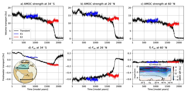
To determine optimal regions for the prediction of an AMOC collapse in this CESM simulation, we branched off two simulations from the quasi-equilibrium simulation [18]. The two simulations have a different but constant freshwater forcing and we refer to them as ( Sv, blue curves branched off from model year 600) and ( Sv, red curves branched off from model year 1500); both simulations are integrated for 500 years. The simulations and equilibrate after about 300 years and are almost in statistical equilibrium in the remaining part of the simulation. The value of at 34∘S for is 0.06 Sv (last 50 years) which is close to the quasi-equilibrium simulation value of 0.10 Sv (model years 575 – 625). Values of for drift away a bit more, with a time mean at 34∘S of -0.16 Sv (last 50 years), compared to -0.10 Sv in the quasi-equilibrium simulation (model years 1475 – 1525). The values at 26∘N and 60∘N for and remain very close to their branching point values. As at 34∘S is considered an important indicator for AMOC stability [4], the simulation has a lower value of at 34∘S and is closer to the tipping point than . Hence we expect that (classical) EWS would show stronger signals of critical slowdown in than in .
To quantify the ratio of the EWS calculated from and , we use yearly averaged and linearly detrended data from model years 350 – 500 where the simulations are best equilibrated. A sliding window of 70 years is used (the results are robust when using a window of 60-80 years) and the average ratio over all possible permutations is computed according to:
| (1) |
where years, indicates the type of EWS, the sliding window size (70 years), and either the temperature () or the salinity (). Locations with for (variance) and (lag-1 autocorrelation) are signatures of a stronger critical slowdown in . The null-hypothesis that is rejected when the probability . Furthermore, a requirement that the value of the is applied in order to avoid large values of due to low values.
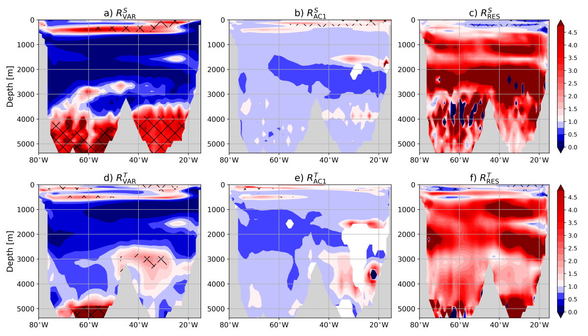
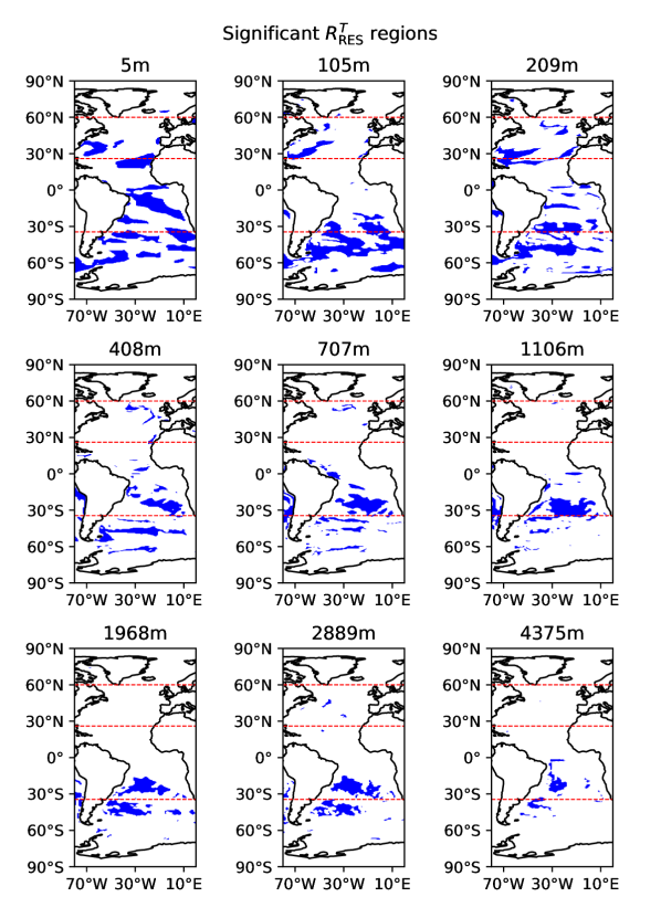
Values of and are shown in Figure 2 along the SAMBA transect at 34∘S for salinity (panels a,b) and temperature (panels d,e). The quantity distinctly shows two bands of significant values, one just below the surface ranging to 1000 m (i.e., Atlantic Surface Water and Antarctic Intermediate Water), and the other on the western part of the transect ranging between 2000 m and 3000 m depth (i.e., North Atlantic Deep Water). The value of indicates a significantly larger variance in compared to in almost the entire western part of the transect. The values of and predominantly show significance in the western part, while the eastern part is characterised by too low AC1 values.
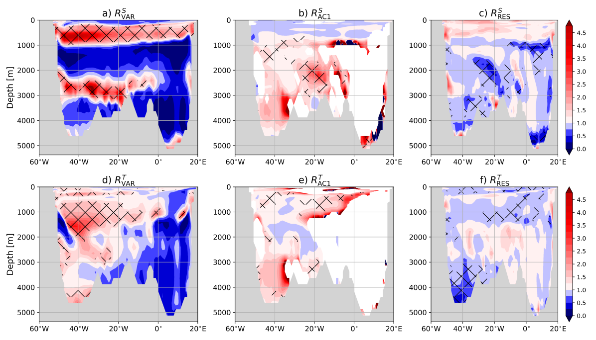
One would expect that classical EWS (i.e., variance and lag-1 autocorrelation) consistently identify regions where the AMOC in CESM shows signs of critical slowdown. There is indeed some overlap between significant and regions along the SAMBA transect. However, these EWS are highly influenced by changes in properties of the noise [9] which may be problematic in their consistency. Unlike and , the restoring rate (see Methods) is less influenced by the properties of the noise, making it a more robust statistical indicator for critical slowdown detection [9]. Note that according to EWS theory (see Methods), decreases when approaching a saddle-node bifurcation and reaches zero from below at the tipping point. Values of and (Figures 2c,f) are significantly smaller than 1 (again ) at intermediate depths in the center of the SAMBA section and near the bottom in the west. There are a few regions along the SAMBA transect where all three EWS ratios are (significantly) indicating a critical slowdown and they are mainly found below 500 m depths. This result is robust when slightly varying the latitude of the section in the South Atlantic (results not shown).
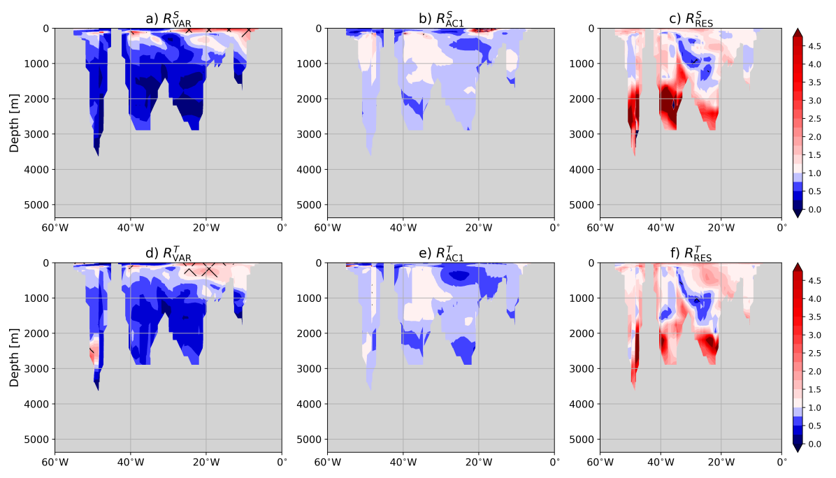
There are almost no regions in the North Atlantic where all three EWS ratios show indications of critical slowdown. EWS ratios for the RAPID transect (26∘N, Figure S1) and OSNAP transect (60∘N, Figure S2) suggest that the statistical indicators along these measurement transects are not effectively detecting or indicating a critical slowdown when approaching the AMOC collapse in the CESM. A possible explanation might be that the signal to noise ratio is too low such that the signal is not captured well enough. Basin-wide plots of the ratios (Figure S3) and (Figure S4) at different depths indicate substantially more significant regions in the South Atlantic than in the North Atlantic. From the equilibrium simulations and it can therefore be concluded that values of and along the 34∘S transect are the most effective in measuring a critical slowdown of the AMOC.
Earlier analysis [19, 20] also focused on classical EWS using data from a FAMOUS model simulation [21], which showed an AMOC collapse under a relatively rapid freshwater forcing change with a rate of 5 10-4 Sv yr-1. The results of [19] show that the variance and lag-1 autocorrelation in the annual resolution data are most reliable in the high northern latitudes and at the southern boundary of the Atlantic. However, the analysis of [20] indicates no early warning signs in the variance and lag-1 autocorrelation using the same model, which is more in agreement to the analysis provided here. Although [20] uses a different method than [19] and averages the data over the latitudes, they only find a strong anomalous signal in the kurtosis indicator when combining AMOC data along several latitudinal transects in the North and South Atlantic, including the RAPID and SAMBA transects. Our equilibrium analysis suggests a robust EWS along one transect only, namely the 34∘S transect, making it a more easily computable EWS compared to the complex network based one in [20].
Tipping Times
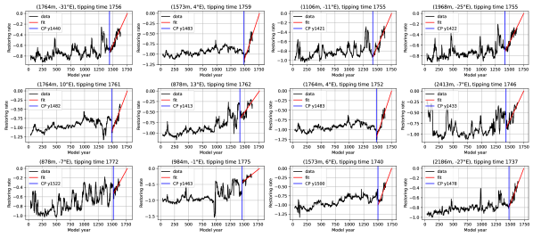
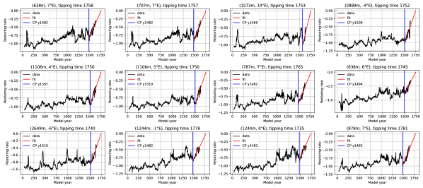
We next test whether data of the 34∘S transect of the quasi-equilibrium CESM simulation can be used to determine the tipping time, i.e. the time that the AMOC collapses. Here, we assume, based on the EWS theory, that the tipping time is associated with a zero restoring rate (see Methods). First, we determine the local restoring rate over the quasi-equilibrium simulation, with a sliding window of 70 years where the data is linearly detrended. The restoring rate time series are limited to model year 1635, i.e. the last sliding window covers model years 1600 – 1670. In this way, the AMOC collapse is excluded from the analysis. Next, we determine the change point (CP), based on a change in the statistical properties of the given time series (see Methods), in the interval between model years 1300 and 1600. To address the robustness of the CP analysis, we allow the CP to vary between model year 1300 and CPend, where CPend varies between model year 1500 and 1600. Data from the CP to model year 1635 are used to linearly fit the restoring rates which are then extrapolated to zero to find (Figures S5 and S6).
A linear fit at a particular grid point is only included for estimation of the tipping time when the time series increases (significantly) monotonically (see Methods) and when the value (as determined from the simulations and ) is significant (Figures 2c,f). The PDFs of the tipping times using these grid points are shown in Figures 3b,d. We find that the median of the estimated AMOC tipping time (Figure 3) is model year 1787 (1688 – 2082, 10 and 90% percentiles, respectively) for the largest CPend value. Using a similar approach, [4] found the actual AMOC tipping time at model year 1758 (1741 – 1775, 10% and 90% percentiles, respectively). Hence, a reasonable AMOC tipping time estimate is found using the locations for which is significant. The actual AMOC tipping time falls inside the 25% to 75% percentile and is robust for varying CPend. However, for temperature, using in a similar way to determine the grid points for the linear fits, this estimate is model year 1959 (1750 – 2291, 10 and 90% percentiles, respectively) and hence is not close to the AMOC tipping time.
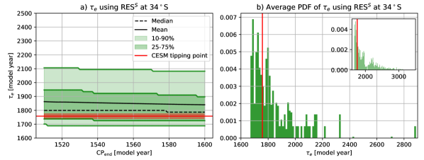
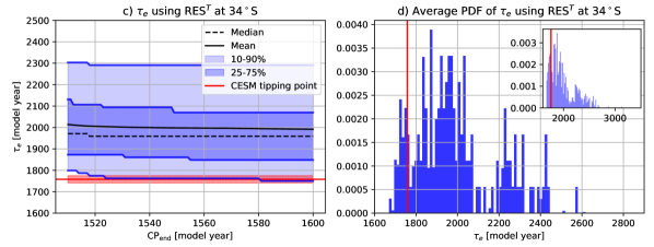
When we consider all (i.e., significant and non-significant ) grid points for the estimate and apply the same criteria for the fits, the tipping time PDF shifts to later years (inset in Figure 3b). The actual AMOC tipping time still falls inside the 25% to 75% percentile and is also robust for varying CPend (not shown). The estimate from temperature restoring rates is improving slightly when we consider all grid points (inset in Figure 3d). Applying the same analysis on the RAPID and OSNAP transects results in an inconsistent estimate for the AMOC tipping time. For example, most grid points (with a significant or ) show no CP in the restoring rate time series. For the grid points where a fit was obtained, the 10% percentile of the PDF estimate was 100 years later than the actual AMOC tipping time.
It is interesting that a useful tipping time estimate can only be obtained using data from about model year 1300 and the methodology fails when earlier model data are used. This is thought to be connected to the fact that the AMOC-induced freshwater convergence is negative [4] only after model year 1300. As this freshwater convergence (approximately equal to at 34∘S) is a measure of the salt-advection feedback, the AMOC starts to decrease due to internal feedbacks only after model year 1300. Because from observations the present-day AMOC has a negative freshwater convergence [22, 23], we next perform a comparable analysis on reanalysis data.
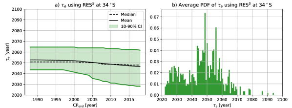
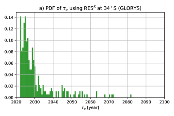
Using the physics-based observable at 34∘S [4], it turned out to be impossible to estimate the tipping time from reanalysis data. The approach above, however, provides a new way to estimate such a tipping time and we apply it next on salinity data along the SAMBA transect for the reanalysis products ORAS5, GLORYS and SODA. The ORAS5 reanalysis dataset runs from 1958 to 2023, and to address robustness we vary CPend between 1978 to 2017. The restoring rate is determined using a sliding window of 10 years. Slightly shorter (more noise) and longer window (data limitation) lengths give similar results but due to the short noisy time series cannot be varied much. We use all section data in the estimation of the tipping time, as otherwise a too small number of data points would remain.
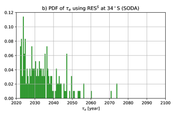
The mean AMOC tipping time estimate from ORAS5 is year 2050 and is robust to varying CPend (Figure 4a). The earliest year (mean 10% percentile level) for a potential AMOC collapse is 2037 and the latest year (mean 90% percentile level) is 2064. The average probability of an AMOC collapse before the year 2050 is with a standard deviation of 17% for ORAS5 (cf. Figure 4b). Applying the same procedure to SODA and GLORYS results in 91% and 92% collapse probabilities before 2050, respectively (Figure S7). Note that these latter two reanalysis data sets have an even shorter length than ORAS5 and are therefore less reliable.
Discussion
In the IPCC-AR6 report, the probability of an AMOC collapse is considered to be low with medium confidence [24]. Our analysis provides a first probability estimate from reanalysis data which gives a mean tipping time estimation of 2050 with a 10 – 90% CI of 2037 – 2064. This is comparable to the findings of [10] who used the sub-polar SST index to estimate the AMOC tipping time to be at 2057, with a 95% confidence interval 2025 – 2095. Interestingly, the sub-polar SST index does not give an early warning signal for the AMOC collapse in the CESM quasi-equilibrium simulation [4] and the sub-polar gyre is also not identified here as an optimal observational region. Considering the problems with EWS detection using proxy based AMOC time series [12], the tipping time estimate correspondence may just be coincidental. To establish the results presented in this paper, several assumptions were made, which require further justification.
First, the CESM quasi-equilibrium simulation showing the AMOC collapse is for a pre-industrial situation with relatively high freshwater forcing. This is obviously far outside the parameter regime of historical observations and mainly due to biases in this model [23], in particular in the Indian Ocean freshwater fluxes. We assume that for developing the optimal observation regions, the different background states do not matter. This is plausible as the physical mechanism of the collapse, and the associated physical variables involved, are independent of background conditions. This justifies our methodology of determining the tipping time distribution from reanalysis data.
Second, the quality of the reanalysis data is questionable for determining the collapse time distribution because these products also depend on models that have their biases. Furthermore, the time series are relatively short compared to the SST based AMOC reconstructions [8]. On the positive side, the reanalyses show consistently lower biases compared to real observations than global climate models, in particular those related to the AMOC, such as the at 34∘S [4]. Although the assumption that reanalyses data are adequate here for tipping time estimation can not be fully justified, they are at the moment the best observational products which are available.
Third, the analysis provided here assumes that by extrapolating the restoring rate to zero, one can find the location of the tipping time of the system. While this is theoretically true when the rate of forcing is much smaller than the equilibration time scales of the AMOC, in both the CESM simulation and the observations there will be an overshoot present depending on the forcing rate [25]. Furthermore, the overshoot can be different in the reanalysis data compared to the quasi-equilibrium simulation, giving an additional uncertainty. Also because we use all section grid points and not only significant ones for the reanalysis data (cf. Figure 3c), our method can only provide a lower bound of the tipping time and it is difficult to determine an uncertainty measure. Additionally, the future forcing can be highly non-linear [26], which can also affect the tipping time.
Although there has been criticism regarding the estimation of tipping times from observational data and the various assumptions inherent in the estimation procedures [12], our method presented here offers a more physically based approach to identify optimal locations for EWS and establishing a lower bound of AMOC tipping times. By focussing on the restoring rate in our critical slowdown analysis, we address the issues of the possibly non-stationary and/or non-white noise forcing of the AMOC [27].
Our analysis of the CESM results indicates that the SAMBA (S) transect data, in particular the salinity, are most useful for providing (and improving the current) estimates of AMOC tipping probabilities. This result is consistent with the recently [4] identified physics-based indicator of an AMOC collapse ( at 34∘S). Our work therefore leads to two major conclusions. Observations at the southern boundary of the Atlantic appear crucial for early warning of an AMOC collapse. As a consequence, the SAMBA measurements are important to continue over the next few decades. Second, the probability of an AMOC collapse before the year 2100 is very likely to be underestimated in the IPCC-AR6 and needs to be reconsidered in the IPCC-AR7.
Methods
Climate Model Simulations
We use simulation results of the CESM version 1.0.5 (the f19g16 configuration) with horizontal resolutions of 1∘ for the ocean/sea-ice and 2∘ for the atmosphere/land components. In [28], results from a quasi-equilibrium simulation were presented, which was branched off from the pre-industrial CESM control simulation at model year 2,800 [29]. The quasi-equilibrium simulation was performed by linearly increasing the surface freshwater forcing between latitudes 20∘N and 50∘N with a rate of 3 10-4 Sv yr-1 up to model year 2,200, where it reaches a freshwater flux forcing of = 0.66 Sv. The freshwater flux anomaly was globally compensated to conserve salinity. From the quasi-equilibrium simulation, two new simulations were performed: one starting at model year 600 under constant = 0.18 Sv and one starting at model year 1500 under constant = 0.45 Sv. These simulations were continued for 500 model years where the states are in near statistical equilibrium.
The Freshwater Transport
The freshwater transport of the overturning component () at latitude and time is determined as:
| (2) |
where g kg-1 is a reference salinity. The is defined as ,
where is the meridional velocity and the full-depth section spatially-averaged meridional velocity.
The quantity indicates the zonally-averaged salinity.
The Restoring Rate
Classical EWS are based on a representation of the behaviour of perturbations on a statistical equilibrium state under white noise near a saddle node-bifurcation. This is defined by an Ornstein-Uhlenbeck process and can in the one-dimensional case be expressed by:
| (3) |
where represents the time-dependent state variable, the restoring rate, the variance of the noise and the noise process. The restoring rate characterises the resilience of the system, and as the system moves towards a tipping point, the restoring rate will decrease. A negative value of represents a stable system state, and a saddle-node bifurcation point can be marked as the point where reaches zero from below.
From a discrete time series with sampling time , the stationary variance (VAR) and lag-1 autocorrelation (AC1) in case is a white noise process are given by and , respectively, where . Hence, when , and the variance will become unbounded.
However, in many time series, variations in variance and autocorrelation can also be related to increasing variance and autocorrelation of the external noise that forces the system, unrelated to critical slowdown, and therefore a modified EWS is used in [9].
The restoring rate , indicated by RES, which directly quantifies the stability of the system, can be inferred from a regression of onto under the assumption of autocorrelated residual noise with the autoregression coefficient as a free parameter.
In this way, the estimation of RES is insensitive to increasing variance and autocorrelation of the noise and provides a robust indicator for a system approaching a saddle-node. We therefore determine, in addition to the variance and lag-1 autocorrelation, also the restoring rate of the time series using the procedure of [9].
Change Points and Restoring Rate Fits The change point (CP) analysis is applied to the restoring rate time series. The CP analysis detects changes in the mean and slope of the time series. The minimum improvement in total residual error is set to 1 in order to limit the amount of returned change points and only get the most pronounced ones of the time series. The data is linearly fitted between the CP and the remaining part of the time series. A Kendall-tau test with 1000 Fourier surrogates is performed on the restoring rate fit and only the ones with and are kept. In this way, only highly correlated fits which are statistically significant and increasing over time are selected.
Acknowledgments
The model simulation and the analysis of all the model output was conducted on the Dutch National Supercomputer Snellius within NWO-SURF project 17239. We thank Michael Kliphuis (IMAU, UU) for carrying out these simulations and his support in analysing the data.
Declarations
-
•
Funding – E.J.V.S. is funded by Utrecht University, R.M.v.W. and H.A.D. are funded by the European Research Council through the ERC-AdG project TAOC (project 101055096).
-
•
Conflict of interest – The authors declare no competing interest
-
•
Ethics approval – Not applicable
-
•
Availability of data and materials – The (processed) model output will be made available on Zenodo upon publication. The reanalysis and assimilation products can be accessed through: ORAS5 (https://doi.org/10.24381/cds.67e8eeb7), GLORYS12V1 (https://doi.org/10.48670/moi-00021) and SODA3.15.2 (http://www.soda.umd.edu).
-
•
Code availability – The analysis scripts will be made available on Zenodo upon publication.
-
•
Authors’ contributions – E.J.V.S., R.M.v.W. and H.A.D. conceived the idea for this study. E.J.V.S conducted the analysis and prepared all figures. All authors were actively involved in the interpretation of the analysis results and the writing process.
References
- \bibcommenthead
- Rahmstorf [2002] Rahmstorf, S.: Ocean circulation and climate changes during the past 120,000 years. Nature 419, 207–214 (2002)
- Armstrong McKay et al. [2022] Armstrong McKay, D.I., Staal, A., Abrams, J.F., Winkelmann, R., Sakschewski, B., Loriani, S., Fetzer, I., Cornell, S.E., Rockström, J., Lenton, T.M.: Exceeding 1.5 C global warming could trigger multiple climate tipping points. Science 377(6611), 7950 (2022)
- Orihuela-Pinto et al. [2022] Orihuela-Pinto, B., England, M.H., Taschetto, A.S.: Interbasin and interhemispheric impacts of a collapsed Atlantic Overturning Circulation. Nature Climate Change 12(6), 558–565 (2022)
- van Westen et al. [2024] Westen, R.M., Kliphuis, M., Dijkstra, H.A.: Physics-based early warning signal shows that AMOC is on tipping course. Science Advances 10(6) (2024) https://doi.org/10.1126/sciadv.adk1189
- Ganopolski and Rahmstorf [2001] Ganopolski, A., Rahmstorf, S.: Rapid changes of glacial climate simulated in a coupled climate model. Nature 409, 153–158 (2001)
- Vettoretti et al. [2023] Vettoretti, G., Ditlevsen, P., Jochum, M., Rasmussen, S.O.: Atmospheric CO2 control of spontaneous millennial-scale ice age climate oscillations. Nature Geoscience 15, 300–306 (2023)
- Frajka-Williams et al. [2019] Frajka-Williams, E., Ansorge, I.J., Baehr, J., Bryden, H.L., Chidichimo, M.P., Cunningham, S.A., Danabasoglu, G., Dong, S., Donohue, K.A., Elipot, S., Heimbach, P., Holliday, N.P., Hummels, R., Jackson, L.C., Karstensen, J., Lankhorst, M., Le Bras, I.A., Susan Lozier, M., McDonagh, E.L., Meinen, C.S., Mercier, H., Moat, B.I., Perez, R.C., Piecuch, C.G., Rhein, M., Srokosz, M.A., Trenberth, K.E., Bacon, S., Forget, G., Goni, G., Kieke, D., Koelling, J., Lamont, T., McCarthy, G.D., Mertens, C., Send, U., Smeed, D.A., Speich, S., Berg, M., Volkov, D., Wilson, C.: Atlantic meridional overturning circulation: Observed transport and variability. Frontiers Media S.A. (2019). https://doi.org/10.3389/fmars.2019.00260
- Caesar et al. [2018] Caesar, L., Rahmstorf, S., Robinson, A., Feulner, G., Saba, V.: Observed fingerprint of a weakening Atlantic Ocean overturning circulation. Nature 556(7700), 191–196 (2018) https://doi.org/10.1038/s41586-018-0006-5
- Boers [2021] Boers, N.: Observation-based early-warning signals for a collapse of the Atlantic Meridional Overturning Circulation. Nature Climate Change 11(8), 680–688 (2021) https://doi.org/10.1038/s41558-021-01097-4
- Ditlevsen and Ditlevsen [2023] Ditlevsen, P., Ditlevsen, S.: Warning of a forthcoming collapse of the Atlantic meridional overturning circulation. Nature Communications 14(1), 4254 (2023)
- Ditlevsen and Johnsen [2010] Ditlevsen, P.D., Johnsen, S.J.: Tipping points: Early warning and wishful thinking. Geophysical Research Letters 37(19), 19703 (2010)
- Ben-Yami et al. [2023] Ben-Yami, M., Morr, A., Bathiany, S., Boers, N.: Uncertainties too large to predict tipping times of major Earth system components (2023)
- Rolland [2018] Rolland, J.: Extremely rare collapse and build-up of turbulence in stochastic models of transitional wall flows. Physical review. E 97, 2–1 (2018)
- Castellana et al. [2019] Castellana, D., Baars, S., Wubs, F.W., Dijkstra, H.A.: Transition probabilities of noise-induced transitions of the Atlantic Ocean circulation. Scientific Reports 9(1), 20284 (2019)
- Castellana and Dijkstra [2020] Castellana, D., Dijkstra, H.A.: Noise-induced transitions of the Atlantic Meridional Overturning Circulation in CMIP5 models. Scientific Reports 10(1), 1–9 (2020)
- Baars et al. [2021] Baars, S., Castellana, D., Wubs, F.W., Dijkstra, H.A.: Application of adaptive multilevel splitting to high-dimensional dynamical systems. Journal of Computational Physics 424, 109876 (2021) https://doi.org/10.1016/j.jcp.2020.109876 2011.05745
- Cini et al. [2024] Cini, M., Zappa, G., Ragone, F., Corti, S.: Simulating AMOC tipping driven by internal climate variability with a rare event algorithm. npj Climate and Atmospheric Science 7(1) (2024) https://doi.org/10.1038/s41612-024-00568-7
- van Westen et al. [2024] Westen, R.M., Jacques-Dumas, V., Boot, A.A., Dijkstra, H.A.: The Role of Sea-ice Processes on the Probability of AMOC Transitions. arXiv preprint arXiv:2401.12615 (2024)
- Boulton et al. [2014] Boulton, C.A., Allison, L.C., Lenton, T.M.: Early warning signals of atlantic meridional overturning circulation collapse in a fully coupled climate model. Nature Communications 5 (2014) https://doi.org/10.1038/ncomms6752
- Feng and Dijkstra [2014] Feng, Q.Y., Dijkstra, H.: Are North Atlantic multidecadal SST anomalies westward propagating? Geophysical Research Letters 41, 541–546 (2014) https://doi.org/10.1002/2013GL058687
- Hawkins et al. [2011] Hawkins, E., Smith, R.S., Allison, L.C., Gregory, J.M., Woollings, T.J., Pohlmann, H., De Cuevas, B.: Bistability of the Atlantic overturning circulation in a global climate model and links to ocean freshwater transport. Geophysical Research Letters 38(10), 10605 (2011)
- Weijer et al. [2019] Weijer, W., Cheng, W., Drijfhout, S.S., Fedorov, A.V., Hu, A., Jackson, L.C., Liu, W., McDonagh, E., Mecking, J., Zhang, J.: Stability of the Atlantic Meridional Overturning Circulation: A review and synthesis. Journal of Geophysical Research: Oceans 124(8), 5336–5375 (2019)
- Van Westen and Dijkstra [2024] Van Westen, R.M., Dijkstra, H.A.: Persistent climate model biases in the Atlantic Ocean’s freshwater transport. Ocean Science 20(2), 549–567 (2024) https://doi.org/10.5194/os-20-549-2024
- Masson-Delmotte et al. [2021] Masson-Delmotte, V., Zhai, P., Chen, Y., Goldfarb, L., Gomis, M.I., Matthews, J.B.R., Berger, S., Huang, M., Yelekçi, O., Yu, R., Zhou, B., Lonnoy, E., Maycock, T.K., Waterfield, T., Leitzell, K., Caud, N.: The Physical Science Basis Summary for Policymakers Technical Summary Frequently Asked Questions Glossary Part of the Working Group I Contribution to the Sixth Assessment Report of the Intergovernmental Panel on Climate Change Edited By, (2021). www.ipcc.ch
- Ritchie et al. [2021] Ritchie, P.D.L., Clarke, J.J., Cox, P.M., Huntingford, C.: Overshooting tipping point thresholds in a changing climate. Nature Research (2021). https://doi.org/10.1038/s41586-021-03263-2
- Riahi et al. [2017] Riahi, K., Vuuren, D.P., Kriegler, E., Edmonds, J., O’Neill, B.C., Fujimori, S., Bauer, N., Calvin, K., Dellink, R., Fricko, O., Lutz, W., Popp, A., Cuaresma, J.C., KC, S., Leimbach, M., Jiang, L., Kram, T., Rao, S., Emmerling, J., Ebi, K., Hasegawa, T., Havlik, P., Humpenöder, F., Da Silva, L.A., Smith, S., Stehfest, E., Bosetti, V., Eom, J., Gernaat, D., Masui, T., Rogelj, J., Strefler, J., Drouet, L., Krey, V., Luderer, G., Harmsen, M., Takahashi, K., Baumstark, L., Doelman, J.C., Kainuma, M., Klimont, Z., Marangoni, G., Lotze-Campen, H., Obersteiner, M., Tabeau, A., Tavoni, M.: The Shared Socioeconomic Pathways and their energy, land use, and greenhouse gas emissions implications: An overview. Global Environmental Change 42, 153–168 (2017) https://doi.org/10.1016/j.gloenvcha.2016.05.009
- Boettner and Boers [2022] Boettner, C., Boers, N.: Critical slowing down in dynamical systems driven by nonstationary correlated noise. Physical Review Research 4(1) (2022) https://doi.org/10.1103/PhysRevResearch.4.013230
- van Westen and Dijkstra [2023] Westen, R.M., Dijkstra, H.A.: Asymmetry of AMOC Hysteresis in a State-Of-The-Art Global Climate Model. Geophysical Research Letters 50(22) (2023) https://doi.org/10.1029/2023GL106088
- Baatsen et al. [2020] Baatsen, M., Von Der Heydt, A.S., Huber, M., Kliphuis, M.A., Bijl, P.K., Sluijs, A., Dijkstra, H.A.: The middle to late Eocene greenhouse climate modelled using the CESM 1.0.5. Climate of the Past 16(6), 2573–2597 (2020)
Supplementary Figures
|
 |