A Clipped Trip: the Dynamics of SGD with Gradient Clipping in High-Dimensions

Abstract

The success of modern machine learning is due in part to the adaptive optimization methods that have been developed to deal with the difficulties of training large models over complex datasets. One such method is gradient clipping: a practical procedure with limited theoretical underpinnings. In this work, we study clipping in a least squares problem under streaming SGD. We develop a theoretical analysis of the learning dynamics in the limit of large intrinsic dimension—a model and dataset dependent notion of dimensionality. In this limit we find a deterministic equation that describes the evolution of the loss. We show that with Gaussian noise clipping cannot improve SGD performance. Yet, in other noisy settings, clipping can provide benefits with tuning of the clipping threshold. In these cases, clipping biases updates in a way beneficial to training which cannot be recovered by SGD under any schedule. We conclude with a discussion about the links between high-dimensional clipping and neural network training.

1 Introduction

Stochastic gradient descent (SGD) methods are the standard for nearly all large scale modern optimization tasks. Even with the ever growing complexities of neural nets, with sufficient hyper-parameter tuning, SGD often outperforms other more complex methods. To deal with the difficulties of training large models over complex datasets, adaptive SGD methods have been developed. One of the simplest such methods is gradient clipping [1, 2]. Gradient clipping replaces any stochastic gradient $\nabla_{\bm{\theta}}f_{\bm{\theta}}(\mathbf{x})$ with a clipped gradient $\operatorname{clip}_{c}(\nabla_{\bm{\theta}}f_{\bm{\theta}}(\mathbf{x}))$, for some threshold $c$, where

$$\operatorname{clip}_{c}(\mathbf{z})=\min\left(1,\frac{c}{\|\mathbf{z}\|}\right)\mathbf{z}.$$ (1)

While gradient clipping was first introduced to address the problem of exploding gradients in recurrent neural networks, it has become an integral part of training models for NLP [3]. It has also found use in other domains such as differential privacy [4, 5] and computer vision [6, 7].

Despite widespread use, the reasons behind the effectiveness of clipping remain somewhat a mystery. For instance, it is unclear exactly how the gradient distribution affects training, or for which distributions clipping can offer benefits. It is hypothesized that the distribution of the gradient norms plays a large role [8]. Also, it is unknown how one should adjust the clipping threshold as the problem scales. There has been growing interest in how models and their optimal hyper-parameters scale with dimension [9]. Understanding this behaviour would allow one to perform hyperparameter tuning on smaller, more efficient models before scaling to a potentially very large final architecture.

In this work we develop a theory of clipped SGD in high-dimensions under the mean-squared error loss (MSE) over a class of random least-squares problems. After formally introducing the class of considered problems (Sec. 2), we show the following:

• In high-dimensions the dynamics of clipped SGD (C-SGD) are well described by an SDE, clipped homogenized SGD (C-HSGD). We provide a non-asymptotic bound on the difference of the risk curves between C-SGD and C-HSGD. Under C-HSGD the risk evolution can be described by a system of ODEs (Sec. 3).

• Using C-HSGD, we show that the differences between clipped and unclipped SGD can be described by two unitless reduction factors $\mu$ and $\nu$ which encode the effect of clipping (Sec. 3).

• The reduction factors control the stability of the algorithm. They describe the precise clipping-learning rate combinations which are convergent. Moreover, we identify some clipping schedules that improve stability (Sec. 4).

• We find a general criterion for when clipping can speed up optimization, described by a different ratio of the reduction factors. We then identify a problem setup where clipping never helps as well as one where clipping improves performance. (Sec. 5).

We conclude with a discussion about the links between our analysis and quantities measurable in real neural networks.

Related work:

The distribution of noise in stochastic gradients and its effect on training was studied by [8]. They argue that this noise is well approximated by a Gaussian for ResNets [10] trained on Imagenet [11], while a heavy-tailed distribution is more appropriate with BERT [12] on an NLP dataset. They show that for heavy-tailed noise unclipped SGD diverges while clipped SGD can converge. Other theoretical analyses on clipping often focus on imposing smoothness conditions on the loss function, and then performing analysis for fixed learning rates [13, 14, 15]. These works have shown that fixed rate clipped SGD can outperform unclipped SGD under certain conditions. Other works have also studied SGD through the lens of SDEs [16, 17, 18]. More recently, partly spurred by the sheer size of modern models as well as the apparent regularity at which they scale [9], there has been an interest in studying stochastic optimization in high-dimensions with SDEs. There is a formal correspondence between the dynamics of learning-relevant quantities like the loss and the trajectory of an equivalent SDE. These relationships have been worked out for SGD in the streaming setup over a variety of losses [19, 20], and the resulting analyses lead to quantities which can be useful for understanding learning dynamics in practical models [21].

2 Problem setup

In this work, we consider linear regression using the mean-squared loss

$$\mathcal{L}(\bm{\theta},\mathbf{x},y)=\|\left\langle\mathbf{x},\bm{\theta}\right\rangle-y\|^{2}/2,$$ (2)

in the streaming or one-pass scenario, where data is not reused. Clipped SGD (C-SGD), without mini-batching, is described by the iteration

$$\bm{\theta}_{k+1} =\bm{\theta}_{k}-\eta_{k}\operatorname{clip}_{c_{k}}\left(\nabla_{\bm{\theta}}\mathcal{L}(\bm{\theta},\mathbf{x},y)\right),$$ (3)

where $\nabla_{\mathbf{x}}\mathcal{L}(\bm{\theta},\mathbf{x},y)=(\left\langle\mathbf{x}_{k+1},\bm{\theta}_{k}\right\rangle-y_{k+1})\mathbf{x}_{k+1}$ with initialization $\bm{\theta}_{0}\in\mathbb{R}{d}$. We assume that the samples $\{(\mathbf{x}_{k},y_{k})\}_{k\geq 0}$, consisting of data $\mathbf{x}_{k}$ and targets $y_{k}$, satisfy the following:

Assumption 1.

The data $\mathbf{x}\in\mathbb{R}{d}$ are Gaussian with covariance $\mathbf{K}$. The targets $y$ are generated by $y=\left\langle\mathbf{x},{\bm{\theta}^{*}}\right\rangle+\epsilon$, where $\epsilon$ represents noise and ${\bm{\theta}^{*}}$ is the ground-truth.

The noise is centered and subgaussian with subgaussian norm $\|\epsilon\|_{\psi_{2}}\leq\dutchcal{v}$ and variance $\mathbb{E}[\epsilon^{2}]=\sigma^{2}$ for some $\dutchcal{v},\sigma\geq 0$.

We formulate a more general version of our results for non-Gaussian data in Appendix A.

Definition 1.

Define the population risk and the noiseless risk:

$$\mathcal{P}(\bm{\theta})=\mathbb{E}_{(\mathbf{x},\epsilon)}\left[(\left\langle\mathbf{x},\bm{\theta}-{\bm{\theta}^{*}}\right\rangle-\epsilon)^{2}\right]/2\quad\text{and}\quad\mathcal{R}(\bm{\theta})=\mathbb{E}_{\mathbf{x}}\left[\left\langle\mathbf{x},\bm{\theta}-{\bm{\theta}^{*}}\right\rangle^{2}\right]/2,$$ (4)

as well as the distance to optimality

$$\mathcal{D}(\bm{\theta})=\|\bm{\theta}-{\bm{\theta}^{*}}\|^{2}.$$

Our theory is phrased in terms of the intrinsic dimension, a statistical notion of dimensionality which is occasionally much smaller than the ambient dimension $\dutchcal{d}$. There are interesting settings where these dimensions are effectively interchangeable, and as such, the reader may wish to, at first glance, consider the results to be phrased in terms of the ambient dimension.

Definition 2 (Intrinsic Dimension).

Let the data $\mathbf{x}\in\mathbb{R}^{\dutchcal{d}}$ have covariance matrix $\mathbf{K}$. Define the intrinsic dimension of the data to be

$$d=\operatorname{Tr}(\mathbf{K})/\|\mathbf{K}\|,$$ (5)

where $\|\mathbf{K}\|$ refers to the operator norm. Note that $d\leq\dutchcal{d}$. We will refer to $\dutchcal{d}$ as the ambient dimension.

Assumption 2.

The covariance matrix $\mathbf{K}$ is normalized such that $\|\mathbf{K}\|=1$. Note that this assumption may always be satisfied by rescaling the problem.

The definition of $d$ can be extended to and measured in real neural networks trained on real datasets; see Appendix C for more details.

We allow for the scheduling of both the clipping threshold and the learning rate. Specifically,

Assumption 3.

There are continuous bounded functions $\eta:\mathbb{R}^{+}\to\mathbb{R}^{+}$ and $c:\mathbb{R}^{+}\to\mathbb{R}^{+}$ such that

$$c_{k}=c(k/d)\sqrt{d} \eta_{k}=\eta(k/d)/d.$$ (6)

We note that while it is reasonable for $c(t)=\infty$ (which is to say that no clipping occurs), for technical reasons, we shall not allow this in our main theorem.

3 Clipped homogenized SGD

Our main result shows that the risk of C-SGD is well-approximated by the solution to an SDE which we call clipped homogenized SGD (C-HSGD):

Definition 3 (Clipped Homogenized SGD).

Denote the stochastic gradient as $\ell_{\bm{\theta}}\mathbf{x}$, where $\ell_{\bm{\theta}}=\left\langle\mathbf{x},\bm{\theta}-{\bm{\theta}^{*}}\right\rangle-\epsilon$. Define the descent reduction factor and the variance reduction factor

$$\mu_{c}(\bm{\theta})=\frac{\|\mathbb{E}[\operatorname{clip}_{c}(\ell_{\bm{\theta}})\mathbf{x}]\|}{\|\mathbb{E}[\ell_{\bm{\theta}}\mathbf{x}]\|}\qquad\text{and}\qquad\nu_{c}(\bm{\theta})=\frac{\mathbb{E}[\operatorname{clip}^{2}_{c}(\ell_{\bm{\theta}})]}{\mathbb{E}[\ell_{\bm{\theta}}^{2}]}.$$ (7)

Then C-HSGD is defined to be the solution to

$$\mathrm{d}\bm{\Theta}_{t}=-\eta(t)\mu_{c(t)}(\bm{\Theta}_{t})\nabla\mathcal{P}(\bm{\Theta}_{t})\mathrm{d}t+\eta(t)\sqrt{\frac{2\nu_{c(t)}(\bm{\Theta}_{t})\mathcal{P}(\bm{\Theta}_{t})\mathbf{K}}{d}}\mathrm{d}B_{t},$$ (8)

where initialization is taken to be the same as SGD and $B_{t}$ is a standard Brownian motion.

This has similar structure to an SDE previously established for unclipped SGD [20], with the addition of reduction factors $\mu_{c}$ and $\nu_{c}$ that capture the effects of clipping. The reduction factors take on values in $[0,1]$ with the limits

$$\lim_{c\to 0^{+}}\mu_{c}=\lim_{c\to 0^{+}}\nu_{c}=0\qquad\text{and}\qquad\lim_{c\to\infty}\mu_{c}=\lim_{c\to\infty}\nu_{c}=1.$$ (9)

In essence, the homogenized SGD suggests that in the limit $d\to\infty$, clipped SGD is still driven by a drift term in the direction of $\nabla_{\bm{\theta}}\mathcal{R}$—but clipping provides a bias against the gradient which shrinks the descent term (hereafter the negative term in (8)). Meanwhile, the diffusion term is shrunk by $\nu_{c}(\theta)$ due to the reduction of variance of the clipped gradients. These terms imply a tradeoff: clipping should aim to reduce variance (decrease $\nu_{c}$) more than it shrinks the descent term (decrease $\mu_{c}$). We investigate this trade-off in detail in Section 5.

Some computed examples of $\mu_{c}$ and $\nu_{c}$ for select data and noise distributions are given in Appendix D. Although computing $\nu_{c}$ is generally straightforward, calculating the risk-coefficient $\mu_{c}$ is often more challenging. However, for Gaussian data, Stein’s Lemma shows that

$$\mu_{c}(\bm{\theta})=\mathbb{P}(|\ell_{\bm{\theta}}|\leq c).$$ (10)

A key point here is that this quantity depends only on the fraction of unclipped gradients.

We now state our main theorem.

Theorem 1.

Suppose that Assumptions 1, 2 and 3 hold. Suppose that $\bm{\Theta}_{t}$ and $\bm{\theta}_{k}$ are independent realizations of C-HSGD and C-SGD with equal, deterministic initial conditions. Let $\overline{c}=\sup_{t}c(t)$ and ${\overline{\eta}}=\sup_{t}{\eta}(t)$. There is a constant $\mathcal{C}=\mathcal{C}(\dutchcal{v},(n/d),\overline{c},\overline{\eta},\|\bm{\theta}_{0}-{\bm{\theta}^{*}}\|^{2})$, a stochastic process $\mathcal{E}$, and a constant $m=m(\dutchcal{v})$ so that for any $1\leq u\leq md$ and any $n$

$$\sup_{0\leq k\leq n}\left\|\begin{bmatrix}\mathcal{R}(\bm{\theta}_{k})\\ \mathcal{D}(\bm{\theta}_{k})\end{bmatrix}-\begin{bmatrix}\mathcal{R}(\bm{\Theta}_{k/d})\\ \mathcal{D}(\bm{\Theta}_{k/d})\end{bmatrix}\right\|\leq\mathcal{C}\mathcal{E}(n/d)u\log(d)d^{-1/2},$$ (11)

with probability $1-e^{-u}$ and provided the right hand side is less than $1$. The stochastic process $\mathcal{E}$ is given by

$$\mathcal{E}(t)=\exp\left(\int_{0}^{t}\frac{C{\eta}(s)^{2}\sigma\,\mathrm{d}s}{\sqrt{\mathcal{R}(\bm{\Theta}_{s})+\mathcal{R}(\bm{\theta}_{sd})}}\right)$$

for an absolute constant $C>0$. The constant $\mathcal{C}$ can be bounded by

$$\mathcal{C}\leq C\sqrt{n/d}\,\overline{\eta}\dutchcal{v}^{2}\cdot((1+\|\bm{\theta}_{0}-{\bm{\theta}^{*}}\|^{2})\dutchcal{v}^{2}+\overline{c}^{2}\sqrt{n/d})\cdot\exp\left(C\max\{\overline{\eta},\overline{\eta}^{2}\}(n/d)\right)$$

for an absolute constant $C>0.$

Informally, this theorem says that

$$\sup_{0\leq k\leq n}\left\|\begin{bmatrix}\mathcal{R}(\bm{\theta}_{k})\\ \mathcal{D}(\bm{\theta}_{k})\end{bmatrix}-\begin{bmatrix}\mathcal{R}(\bm{\Theta}_{k/d})\\ \mathcal{D}(\bm{\Theta}_{k/d})\end{bmatrix}\right\|=\mathcal{O}(\log(d)d^{-1/2}).$$

In particular, as $d$ grows, the risk curves of C-SGD and C-HSGD look closer to one another for longer time windows and with higher probability. Under additional assumptions, such that the C-HSGD curve converges to a dimension-independent deterministic limit, this would show convergence of the risk curves of C-SGD to a dimension-independent limit.

The presence of the $\mathcal{E}(t)$, while not desirable, should also not be alarming: when $\sigma=0$ (recall Assumption 1), this disappears entirely. On the other hand, when $\sigma\neq 0,$ the risk cannot decrease to $0$ too quickly, and so in many setups (for example when $\eta(s)\equiv\eta$), this will be no larger than $e^{m\times(n/d)}$ for a constant $m$ that depends on $\sigma,\overline{\eta},\overline{c}$, with very high probability.

The complete proof is detailed in Appendix B along with the theorem statement and proof for non-Gaussian data.

Extracting deterministic dynamics.

For any twice differentiable function $q$, we have

$$\mathrm{d}q(\bm{\Theta}_{t})=-\eta(t)\mu_{c(t)}(\bm{\Theta}_{t})\nabla\mathcal{P}(\bm{\Theta}_{t})^{T}\nabla q(\bm{\Theta}_{t})\mathrm{d}t+\frac{\eta(t)^{2}}{d}\nu_{c(t)}(\bm{\Theta}_{t})\mathcal{P}(\bm{\Theta}_{t})\operatorname{Tr}(\mathbf{K}\nabla^{2}q)\mathrm{d}t+\mathrm{d}\mathcal{M}_{t},$$ (12)

where $\mathcal{M}_{t}$ is a martingale which vanishes as $d\to\infty$, which is an example of the concentration of measure phenomenon seen throughout high-dimensional probability. Hence, we have a good deterministic approximation for the evolution of $q(\bm{\Theta}_{t})$ by setting $\mathcal{M}_{t}\equiv 0$.

Based on this idea, we can construct a coupled system of ODEs which will describe the dynamics of the risk. A priori this is an infinite system of ODEs, but this difficulty can be avoided through the use of the resolvent formalism $R(z;\mathbf{K})=(\mathbf{K}-z\mathbf{I})^{-1}$ for $z\in\mathbb{C}$. Consider

$$q_{z}(\bm{\Theta}_{t})=\left\langle(\bm{\Theta}_{t}-{\bm{\theta}^{*}})^{\otimes 2},R(z;\mathbf{K})\right\rangle/2.$$ (13)

We use this to define deterministic equivalents $R_{t}$ and $D_{t}$ for $\mathcal{R}(\bm{\Theta}_{t})$ and $\mathcal{D}(\bm{\Theta}_{t})$. Moreover, Theorem 1 holds as written with $(\mathcal{R}(\bm{\Theta}_{t}),\mathcal{D}(\bm{\Theta}_{t}))$ replaced by $(R_{t},D_{t})$ (see Theorem 8 in Appendix F, where we also elaborate on the system of ODEs). A numerical comparison of C-SGD, C-HSGD, and the ODEs is provided in Figure 1.

The situation becomes much simpler when the data have identity covariance (aka isotropic data).

Example 1 (Isotropic data).

When the data is isotropic Gaussian, the $R_{t}$ solves an autonomous ODE:

$$\dot{R}_{t}=-2\eta(t)\mu_{c(t)}R_{t}+\eta(t)^{2}\nu_{c(t)}(R_{t}+\sigma^{2}/2),$$ (14)

where $R_{0}=\mathcal{R}(\bm{\Theta}_{0})$. Here, we have used that since the data is Gaussian, it is possible to express $\mu_{c}$ and $\nu_{c}$ as functions of the risk. As a slight abuse of notation we shall also write $(\mu_{c}(\mathcal{R}(\bm{\theta})),\nu_{c}(\mathcal{R}(\bm{\theta})))$ for $(\mu_{c}(\bm{\theta}),\nu_{c}(\bm{\theta}))$, and we will suppress the dependence where appropriate. In particular, in (14), we have applied $\mu_{c(t)}$ and $\nu_{c(t)}$ to $R_{t}$.

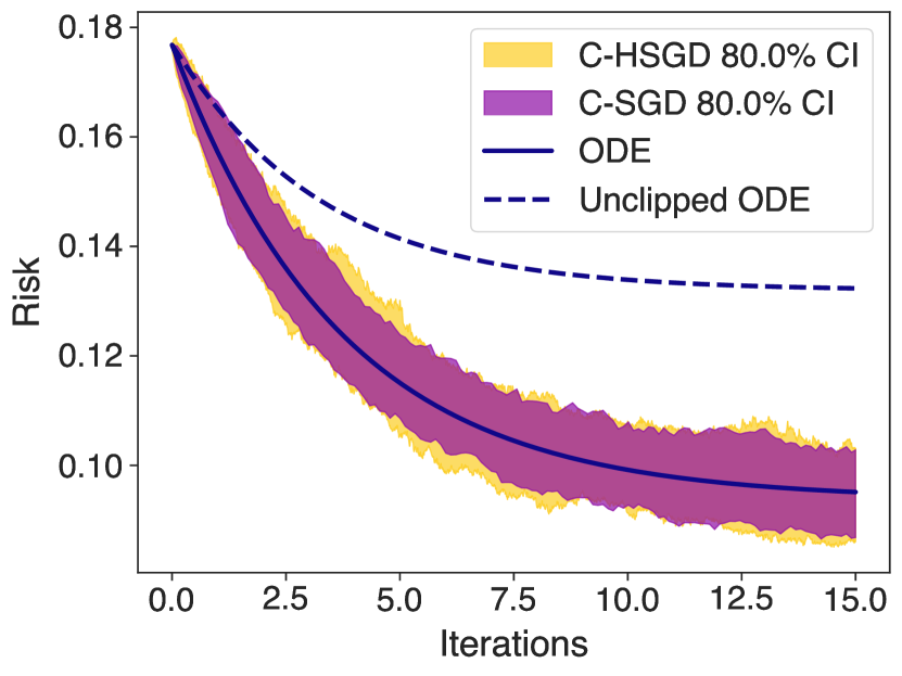
(a) $d=179.74$

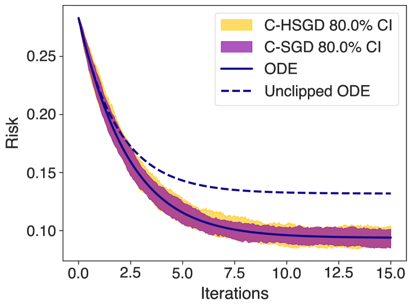
(b) $d=281.63$

Figure 1: Comparison of C-SGD, C-HSGD and their deterministic equivalent (ODE) with Gaussian noise, with the solution to the unclipped ODE for reference. The ambient dimension is $\dutchcal{d}=500$ in both figures, but the intrinsic dimension $d$ changes. The covariance has eigenvalues following a power law $j^{-\alpha},j=1,\ldots,\dutchcal{d}$ with $\alpha=1/5$ and $\alpha=1/9$ for the left and the right figures respectively. We have $\sigma=0.7$, $c_{t}=0.9$, $\eta=0.7$. Plotted is the $80$% confidence interval across $100$ runs.

4 Stability analysis

In this section we establish stability conditions for streaming SGD with clipping. Stability thresholds from convex models are useful for understanding dynamics in deep learning [22, 21]. Additionally, a larger range of stable learning rates can prevent failures in costly training runs. We show that the largest stable learning rate is structurally similar to that of the unclipped SGD case, but with the introduction of the reduction factors $\mu_{c}$ and $\nu_{c}$ which account for the effects of clipping.

From Equation (12), we observe that for either the risk $\mathcal{R}$ or the distance to optimality $\mathcal{D}$, the instantaneous time derivative is quadratic in the learning rate $\eta({t})$. This implies that we can compute a stability threshold for the learning rate, determining whether, in high-dimensions, these measures of suboptimality increase or decrease. We find the critical values $\eta^{*}_{\mathcal{R}}({t})$ and $\eta^{*}_{\mathcal{D}}({t})$ such that $\mathbb{E}[\mathrm{d}\mathcal{R}(\Theta_{t})]=0$ and $\mathbb{E}[\mathrm{d}\mathcal{D}(\Theta_{t})]=0$ . In particular,

$$\eta^{*}_{\mathcal{R}}({t})=\frac{d\|\nabla\mathcal{P}(\bm{\Theta}_{t})\|^{2}}{\operatorname{Tr}(\mathbf{K}^{2})\mathcal{P}(\bm{\Theta}_{t})}\frac{\mu_{c(t)}(\bm{\Theta}_{t})}{\nu_{c(t)}(\bm{\Theta}_{t})}\quad\text{and}\quad\eta^{*}_{\mathcal{D}}({t})=\frac{\mathcal{R}(\bm{\Theta}_{t})}{\mathcal{P}(\bm{\Theta}_{t})}\frac{\mu_{c(t)}(\bm{\Theta}_{t})}{\nu_{c(t)}(\bm{\Theta}_{t})}.$$ (15)

This implies that clipping increases instantaneous stability (for both $\mathcal{R}$ and $\mathcal{D}$) relative to unclipped SGD when

$$\frac{\mu_{c(t)}(\bm{\Theta}_{t})}{\nu_{c(t)}(\bm{\Theta}_{t})}>1.$$ (CSC)

We refer to this as the clipped-stability-criterion (CSC). This can be interpreted as as a relative signal-to-noise-ratio; the fraction of clipped gradients $\mu$ reduces the signal, while clipping reduces the noise through the reduction factor $\nu$. Stability is increased when the relative signal-to-noise-ratio is greater than $1$. Clipping significantly enhances stability when a small fraction of samples contribute disproportionately to the gradient norm.

Clipping will increase the stability of SGD with a small enough choice of $c$:

Theorem 2.

For data $\mathbf{x}\sim N(0,\mathbf{K})$ one may always choose the clipping schedule $c$ small enough to satisfy the (CSC).

The proof of this theorem follows from an application of L’Hôpital’s rule and is available in Appendix E. We provide plots of the (CSC) in Figure 2 under various settings. We conjecture that this result extends beyond Gaussian data, but the current intractability of $\mu$ for general data makes precise claims difficult.

Counterintuitively, clipping can also decrease stability in some cases, when the bias towards $\nabla_{\bm{\theta}}\mathcal{R}$ ($\mu$) is reduced more than the overall gradient norms ($\nu$). This shows that some care must be taken to avoid clipping being detrimental. The proof of the following theorem straightforwardly uses the definitions of $\mu_{c}$ and $\nu_{c}$ and can be found in Appendix E.

Theorem 3.

Consider $\mathbf{x}\sim N(0,\mathbf{K})$ and noise with the distribution given by

$$\mathbb{P}(\epsilon=-\lambda)=p/2, \mathbb{P}(\epsilon=0)=1-p, \mathbb{P}(\epsilon=\lambda)=p/2,$$ (16)

for $p\in(0,1)$ and $\lambda>0$. Then, there is a constant $r$ depending on $p,\lambda$ so that when $R_{t}\leq r$ there always exists $c(t)$ such that the (CSC) is less than $1$. Therefore, clipped SGD can be less stable than unclipped SGD.

5 When does clipped SGD outperform unclipped SGD?

We now ask: under what settings can clipping improve the performance of SGD? Specifically, with the optimal learning rate schedule for unclipped SGD, does there exist a clipping-learning rate combination such that clipping achieves a lower loss at time $T$?

We will use Equation (12) to answer this question. We first present detailed calculations in the isotropic case to find an exact condition on the gradient distribution where clipping improves training. We then show that this condition still applies under anisotropic data. We provide examples and plots of this condition to develop intuition on when clipping helps to improve training.

5.1 Isotropic data

Consider the case of isotropic data where $\mathbf{x}\sim N(0,\mathbf{I})$. Define $R^{\infty}_{t}$ to be the deterministic equivalent of $\mathcal{R}(\bm{\varphi}_{t})$, where $\bm{\varphi}_{t}$ is C-HSGD with $c(t)\equiv\infty$ (which is to say unclipped HSGD). Example 1 shows that $R_{t}$ and $R^{\infty}_{t}$ solve the following ODEs,

$$\frac{\mathrm{d}R_{t}}{\mathrm{d}t}=-2\eta(t)\mu_{c(t)}R_{t}+\frac{\eta^{2}(t)}{2}\nu_{c(t)}(2R_{t}+\sigma^{2}), \frac{\mathrm{d}R^{\infty}_{t}}{\mathrm{d}t}=-2\eta(t)R^{\infty}_{t}+\frac{\eta^{2}(t)}{2}(2R^{\infty}_{t}+\sigma^{2}).$$ (17)

These results enable a comparison between clipped and unclipped SGD. Since these ODEs are quadratic in $\eta(t)$, it is straightforward to greedily maximize their instantaneous rate of descent, resulting in the globally optimal learning rate schedule. Optimizing each ODE over $\eta(t)$ yields

$$\frac{\mathrm{d}R_{t}}{\mathrm{d}t}=-\frac{R_{t}^{2}}{R_{t}+\sigma^{2}/2}\frac{\mu_{c(t)}^{2}}{\nu_{c(t)}} \frac{\mathrm{d}R^{\infty}_{t}}{\mathrm{d}t}=-\frac{\left({R^{\infty}_{t}}\right)^{2}}{R^{\infty}_{t}+\sigma^{2}/2}.$$ (18)

When $R_{t}=R^{\infty}_{t}$, we see that the rate of descent is faster and thus clipping improves SGD exactly when there exists a $c(t)$ such that

$$\frac{\mu^{2}_{c(t)}(R_{t})}{\nu_{c(t)}(R_{t})}>1.$$ (CCC)

We call this inequality the clipping-comparison-criterion (CCC). Therefore, in our setting we can exactly understand when clipping is helpful to training. Informally, the improvement criterion tells us that clipping is effective when it can reduce the variance of the gradient norms, via $\nu_{c(t)}$ more than it reduces the squared reduction to the descent term $\mu^{2}_{c(t)}$. This is consistent with previous observations that, in practice, clipping is effective when the distribution of the gradient norms is heavy-tailed [8], but gives a quantitative rule for comparison. To give some intuition, we provide some plots of these thresholds over various types of noise distributions in Figure 2.

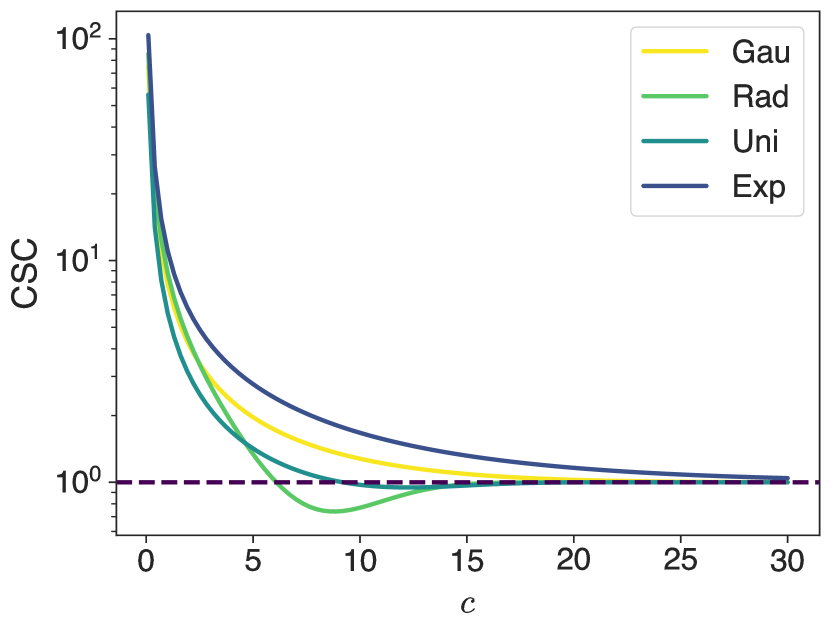
(a) The (CSC)

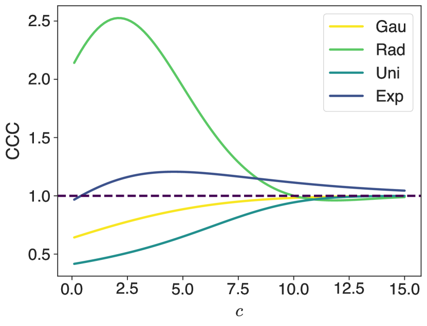
(b) The (CCC)

Figure 2: The (CSC) and (CCC) across various noise distributions: Gaussian (Gau), Rademacher-like (Rad), uniform on $[-M,M]$ (Uni), and symmetrized exponential (Exp) noise. The (CSC) is computed with $R=3,\ \sigma=9,\ p=0.7$; the (CCC) figure uses $R=3,\ \sigma=5,\ p=0.2$ (where $p$ is a parameter for Rademacher-like noise). Parameters are chosen to illustrate different behaviours.

5.2 Anisotropic data

The previous results show that with isotropic data, the optimal clipping schedule can be found by maximizing the (CCC) at each time point. Inspired by this observation, we describe a procedure which, given a learning rate schedule for unclipped SGD, gives us a learning rate-clipping schedule pair which performs at least as well as unclipped SGD—and has a simple condition for showing better performance.

Consider a learning rate schedule $\eta({t})$, used to train unclipped SGD. We define the max-(CCC) clipping threshold schedule as follows: At step $t$, we first set the clipping threshold to

$$c^{*}(t)=\operatorname{argmax}_{c}\frac{\mu^{2}_{c}(R_{t})}{\nu_{c}(R_{t})}.$$ (19)

Given a clipping threshold $c$, we define a compensated learning rate for clipped SGD by

$$\tilde{\eta}(t,c)=\eta(t)/\mu_{c}(R_{t}).$$ (20)

Effectively, this learning rate compensates for the fact that clipping biases SGD against the gradient such that clipped SGD now has the same instantaneous descent term as unclipped SGD. We now choose $\eta^{*}(t)=\tilde{\eta}(t,c^{*}({t}))$ as our learning rate.

The basic idea is that this schedule will never underperform unclipped SGD. If the (CCC) is never satisfied we have $c^{*}({t})\equiv\infty$ and $\eta^{*}(t)=\eta({t})$, recovering the original, unclipped SGD. However, if the (CCC) is satisfied at any time the max-(CCC) schedule will take advantage of this and provide improvements to optimization. In order to show this, we first have to solve for $R_{t}$ under anisotropic data. In this setting, the risk is the sum of two parts: a gradient flow term and an integrated correction term. The gradient flow term is associated with the infinitesimal learning rate limit of SGD. It decreases the risk and comes from solving the underlying problem. The correction term arises because the actual learning rate is not infinitesimal. It encodes the errors made by SGD and increases the risk. Gradient flow is defined to be,

$$\mathrm{d}\bm{\Phi}^{\mathrm{gf}}_{t}=-\nabla\mathcal{R}(\bm{\Phi}^{\mathrm{gf}}_{t})\,\mathrm{d}t,$$ (21)

with $\bm{\Phi}^{\mathrm{gf}}_{0}=\bm{\theta}_{0}$. Then the gradient flow term is $\mathcal{R}(\bm{\Phi}^{\mathrm{gf}}_{t})$. In Appendix F, we show $R_{t}$ with any learning rate $\eta(t)$ and clipping schedule $c(t)$ solves

$$R_{t}=\mathcal{R}(\bm{\Phi}^{\mathrm{gf}}_{\Gamma_{T}^{c}})+\frac{1}{d}\int_{0}^{t}{\eta}^{2}(s)\nu_{c(s)}\operatorname{Tr}(\mathbf{K}^{2}e^{-2\mathbf{K}(\Gamma_{t}^{c}-\Gamma_{s}^{c})})(R_{s}+\sigma^{2}/2)\mathrm{d}s,$$ (22)

where $\Gamma_{t}^{c}=\int_{0}^{t}\eta(s)\mu_{c(s)}ds$ is the clipped integrated learning rate. The integral term in Equation (22) is the finite learning rate correction. The risk of unclipped SGD can be computed using $c(t)\equiv\infty$:

$$R^{\infty}_{t}=\mathcal{R}(\bm{\Phi}^{\mathrm{gf}}_{\Gamma_{T}})+\frac{1}{d}\int_{0}^{t}{\eta}^{2}(s)\operatorname{Tr}(\mathbf{K}^{2}e^{-2\mathbf{K}(\Gamma_{t}-\Gamma_{s})})(R^{\infty}_{s}+\sigma^{2}/2)\mathrm{d}s.$$ (23)

where $\Gamma_{t}=\int_{0}^{t}\eta(s)\mathrm{d}s$. This gives us the following theorem:

Theorem 4.

Given SGD with learning rate schedule $\eta({t})$ and clipped SGD with learning and clipping schedules $\eta^{*}({t})$ and $c^{*}({t})$, then $R_{T}\leq R^{\infty}_{T}$. If there exists a $t\in[0,T]$ such that the (CCC) holds then $R_{T}<R^{\infty}_{T}$. Conversely, if $\mu_{c}^{2}(R)/\nu_{c}(R)\leq 1$ for all $R>0$ and $c>0$, then for any learning and clipping schedules $\eta({t})$ and $c({t})$, SGD with the compensated learning rate schedule $\eta(t)\mu_{c(t)}$ has $R^{\infty}_{T}\leq R_{T}$.

Proof.

With these choices, the clipped risk (22) solves

$$R_{T}=\mathcal{R}(\bm{\Phi}^{\mathrm{gf}}_{\Gamma_{T}})+\frac{1}{d}\int_{0}^{T}\eta^{2}(s)\frac{\nu_{c(s)}}{\mu^{2}_{c(s)}}\operatorname{Tr}(\mathbf{K}^{2}e^{-2\mathbf{K}(\Gamma_{T}-\Gamma_{s})})(R_{s}+\sigma^{2}/2)\mathrm{d}s.$$ (24)

Note that the gradient flow term is identical to that of unclipped SGD. Since the (CCC) is satisfied, the integrated correction term is no larger than unclipped SGD and thus $R_{T}\leq R^{\infty}_{T}$. If the (CCC) occurs at some $t$, then in fact $R_{T}<R^{\infty}_{T}$. For the converse, one substitutes the learning rate schedule into (23) and sees it is smaller than (22). ∎

We note that this result holds for any choice of the unclipped learning rate, even the optimal one. Therefore, if the (CCC) holds at some point along the optimal unclipped SGD trajectory then the benefits of gradient clipping cannot be matched by unclipped SGD.

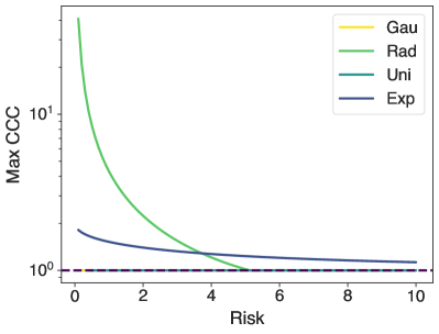
Figure 3: The maximum over $c$ of the (CCC) for various values of the risk. Notice that the maximum value of the $\eqref{eq:clip_comparison_criterion}$ for both uniform and Gaussian noise is $1$, corresponding to unclipped SGD. Plots are computed with $\sigma=7,\ p=0.5$ where $p$ is a parameter in the Rademacher-like noise.

The following theorems give concrete examples of our results and apply in the both the isotropic and anisotropic setting. We show that the (CCC) cannot be satisfied when the data are Gaussian. Then, we show that, as before, broadly distributed gradients can benefit from clipping (even with all finite moments). Both proofs straightforwardly apply the definitions of $\mu_{c}$ and $\nu_{c}$ (Appendix E).

Theorem 5.

If $\mathbf{x}\sim N(0,\mathbf{K})$ and $\epsilon\sim N(0,\sigma^{2})$ then $\mu_{c}^{2}(R)/\nu_{c}(R)\leq 1$ for all $R,c>0$.

Hence, in this case clipped SGD never improves over unclipped SGD (in the sense of Theorem 4).

Theorem 6.

Consider $\mathbf{x}\sim N(0,\mathbf{K})$ and the Rademacher-like noise as described in Theorem 3. Then, there is an $r>0$ depending on $p$ and $\lambda$ so that when $R_{t}\leq r$ there always exists $c(t)$ such that the (CCC) is satisfied.

It is interesting to note that the (CSC) is automatically satisfied if the (CCC) is, implying that when gradient clipping improves SGD’s performance, it also enhances its stability. This dual benefit suggests that in some settings clipping can be used to achieve both efficient and stable training.

We illustrate these theorems with numerical examples. Comparing constant learning rate SGD to clipped SGD with the max-(CCC) schedule and compensated learning rate, we see no improvement for Gaussian noise (Figure 4a). In contrast, with Rademacher-like noise, clipping with compensated learning rate learns faster and reaches a lower value of the risk (Figure 4b). In practice, computing optimal schedules (for learning rate alone or jointly with clipping schedules) remains challenging and is left for future work.

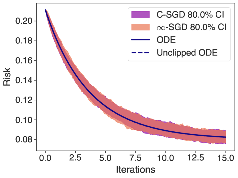
(a) Gaussian noise

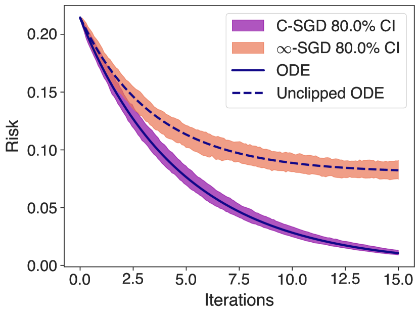
(b) Rademacher-like noise

Figure 4: Results of clipped versus unclipped SGD with anisotropic data under the setting of Theorem 4. The data follow a power law with $d=179.74$ and $\dutchcal{d}=500$. The unclipped learning rate is constantly $\eta=0.4$ while $\sigma=0.8$. We compare Gaussian and Rademacher-like noise with $p=0.2$. Notice that clipping cannot improve SGD in the setting with Gaussian noise while it noticeably improves performance with Rademacher-like noise. SGD is presented with $80$% confidence intervals over $100$ runs.

6 Conclusion

Our analysis of high-dimensional streaming settings shows that the effectiveness of clipping hinges on two key quantities: descent and variance reduction factors $\mu_{c}$ and $\nu_{c}$. The structure of the noise, model, and data then determine the dynamics of $\mu_{c}$ and $\nu_{c}$ for a given clipping threshold. This allows us to compare clipped SGD to unclipped SGD with learning rate and clipping schedules. Clipping can be beneficial in the setting of non-Gaussian noise; in certain noisy regimes, clipping helps filter noisy datapoints more than non-noisy ones. The key is that the gradient norm becomes a strong-enough proxy for the “quality” of a datapoint, and can be used to effectively filter each point.

The local stability of clipped SGD depends on the ratio of $\mu_{c}$ to $\nu_{c}$, the (CSC). The maximum stable learning rate can be increased by clipping if clipping reduces the average square gradient norm more than the probability of clipping. This can be achieved for broad distributions of gradients. Similarly, clipping improves optimization if the ratio of $\mu_{c}^{2}$ to $\nu_{c}$ exceeds $1$, the (CCC). This quantity informs when the tradeoff between biasing training against the gradient and reducing the variance pays off.

One future direction is to consider more complex models and losses. Exact risk curves have been derived in the unclipped SGD setting on more general losses [19]; some of these results are likely adaptable to the clipped SGD setting. Additionally, important quantities from the analysis of high-dimensional linear models can be measured in real networks (via linearization) and can be used to analyze learning dynamics [23]. We believe that the generalized versions of $\mu_{c}$ and $\nu_{c}$ may be interesting to study in real networks.

More generally, our work suggests that operations which filter gradients at the level of individual examples can be beneficial to training. For example, our analysis hints at a possibly more effective strategy of processing large gradients; simply ignore them. This stems from the observation that $\mu_{c}$ would be unchanged by this alternative method, while $\nu_{c}$ would be smaller. Currently, filtering largely happens either during data pre-processing or at the batch level during training due to the limitations of autodifferentiation setups. A promising avenue for future research is to find efficient ways of applying operations like clipping element-wise rather than batch-wise.

Appendix A Full formulation of Theorem 1 with non-Gaussian data

To state the more general version of Theorem 1, we require some additional technical assumptions. Along with all of the assumptions described in Section 2 we will further assume:

Assumption 4.

For some constant $\dutchcal{v}\geq 1$ and any fixed $\bm{\theta}$ with $\|\bm{\theta}\|\leq 1$, we have $\|\mathbf{x}^{T}\bm{\theta}\|_{\psi_{2}}\leq\dutchcal{v}$ and the data satisfy a Hanson-Wright inequality: for all $t\geq 0$ and any fixed matrix $\bm{B}$,

$$\mathbb{P}(|\mathbf{x}^{T}\bm{B}\mathbf{x}-\mathbb{E}[\mathbf{x}^{T}\bm{B}\mathbf{x}]|\geq t)\leq 2\exp\left(-\min\left\{\frac{t^{2}}{\dutchcal{v}^{4}\|\sqrt{\mathbf{K}}\bm{B}\sqrt{\mathbf{K}}\|^{2}_{F}},\frac{t}{\dutchcal{v}^{2}\|\sqrt{\mathbf{K}}\bm{B}\sqrt{\mathbf{K}}\|}\right\}\right),$$ (25)

where $\mathbf{K}$ is the covariance of the data.

Assumption 5.

$\mu$ and $\nu$ satisfy the following Lipschitz-like bounds for some constants $C_{\mu}$ and $C_{\nu}$.

$$|\mu(x)-\mu(y)|\leq C_{\mu}\frac{|\mathcal{R}(x)-\mathcal{R}(y)|}{\min_{z\in\{x,y\}}\mathcal{R}(z)}$$ (26)

$$|\nu(x)\mathcal{P}(x)-\nu(y)\mathcal{P}(y)|\leq C_{\nu}\left(1+\frac{\sigma}{\sqrt{\mathcal{R}(x)+\mathcal{R}(y)}}\right)|\mathcal{R}(x)-\mathcal{R}(y)|$$ (27)

where $\mathcal{R}$ is the risk.

We may now state our more general version of Theorem 1. Here we use $\overline{c}=\max_{t}c(t)$ and $\overline{\eta}=\max_{t}\eta(t)$.

Theorem 7.

There is a constant $\mathcal{C}=\mathcal{C}(\dutchcal{v},(n/d),c,\eta,(1+\|V_{0}\|^{2}))$ and a constant $c=c(\dutchcal{v})$ so that for any $1\leq u\leq cd$

$$\sup_{0\leq k\leq n}\left\|\begin{bmatrix}\mathcal{R}(\bm{\theta}_{k})\\ \mathcal{D}(\bm{\theta}_{k})\end{bmatrix}-\begin{bmatrix}\mathcal{R}(\bm{\Theta}_{k/d})\\ \mathcal{D}(\bm{\Theta}_{k/d})\end{bmatrix}\right\|\leq\mathcal{C}\exp\left(\int_{0}^{n/d}\frac{C_{\nu}\eta^{2}(s)\sigma\,\mathrm{d}s}{\sqrt{\mathcal{R}(\bm{\Theta}_{s})+\mathcal{R}(\bm{\theta}_{sd})}}\right)u\log(d)d^{-1/2},$$ (28)

with probability at least $1-e^{-u}$ and provided the right hand side is less than $1$. The coefficient $\mathcal{C}$ can be bounded by

$$\mathcal{C}\leq C\sqrt{n/d}\overline{\eta}\dutchcal{v}^{2}((1+\|V_{0}\|^{2})\dutchcal{v}^{2}+c^{2}\sqrt{n/d})\exp\left(C\times(1+C_{\mu})\max\{\overline{\eta},\overline{\eta}^{2}\}(n/d)\right)$$

for an absolute constant $C>0.$

We note that when $\sigma=0$ (so there is no noise) we arrive at the simpler conclusion that

$$\sup_{0\leq k\leq n}\left\|\begin{bmatrix}\mathcal{R}(\bm{\theta}_{k})\\ \mathcal{D}(\bm{\theta}_{k})\end{bmatrix}-\begin{bmatrix}\mathcal{R}(\bm{\Theta}_{k/d})\\ \mathcal{D}(\bm{\Theta}_{k/d})\end{bmatrix}\right\|=\mathcal{O}(d^{-1/2}).$$

We note also that if $\eta(s)\equiv\eta$, the risk will be bounded below by a constant that depends only on $\eta,c,\sigma$ with high probability (and provided there is no warm start), and hence again this coefficient can be bounded with high probability in a similar way to $\mathcal{C}$. Moreover, for any desired $d$-independent risk threshold $R_{0}$, if one makes $d$ sufficiently large, then with very high probability, two risk curves will agree up to the point they cross below this risk threshold.

Appendix B Proof of main theorems

In this section we prove both Theorem 1 and Theorem 7.

B.1 Proof of Theorem 1

In order to prove the version of our Theorem with Gaussian data, it suffices to check that Gaussians satisfy both Assumption 4 and 5.

It is a standard fact that the Hanson-Wright inequality is satisfied for Gaussians [24].

Let $z$ be standard Gaussian then recall from (10),

$$\mu_{c}(\bm{\theta}) =\mathbb{P}(|\left\langle\mathbf{x},\bm{\theta}-{\bm{\theta}^{*}}\right\rangle|\leq c)$$ (29)

$$=\mathbb{P}(|\sqrt{2\mathcal{R}(\bm{\theta})}z-\epsilon|\leq c).$$ (30)

With a slight abuse of notation, we condition on $\epsilon$ and use $I=(\epsilon-c,\epsilon+c)$ to express

$$|\mu_{c}(\bm{\theta}_{1})-\mu_{c}(\bm{\theta}_{2})| =\left|\mathbb{P}\left(z\in\frac{I}{\sqrt{2\mathcal{R}(\bm{\theta}_{1})}}\bigg{|}\,\epsilon\right)-\mathbb{P}\left(z\in\frac{I}{\sqrt{2\mathcal{R}(\bm{\theta}_{2})}}\bigg{|}\,\epsilon\right)\right|$$ (31)

$$\leq\left|\mathbb{P}\left(z\leq\frac{c+\epsilon}{\sqrt{\mathcal{R}(\bm{\theta}_{1})}}\bigg{|}\,\epsilon\right)-\mathbb{P}\left(z\leq\frac{c+\epsilon}{\sqrt{\mathcal{R}(\bm{\theta}_{2})}}\bigg{|}\,\epsilon\right)\right|$$ (32)

$$\quad+\left|\mathbb{P}\left(z\leq\frac{c-\epsilon}{\sqrt{\mathcal{R}(\bm{\theta}_{1})}}\bigg{|}\,\epsilon\right)-\mathbb{P}\left(z\leq\frac{c-\epsilon}{\sqrt{\mathcal{R}(\bm{\theta}_{2})}}\bigg{|}\,\epsilon\right)\right|.$$ (33)

Without loss of generality, we assume $c+\epsilon/\mathcal{R}(\bm{\theta}_{2})\leq c+\epsilon/\mathcal{R}(\bm{\theta}_{1})$, then the former term may be bounded by

$$\left|\mathbb{P}\left(z\leq\frac{c+\epsilon}{\sqrt{\mathcal{R}(\bm{\theta}_{1})}}\bigg{|}\,\epsilon\right)-\mathbb{P}\left(z\leq\frac{c+\epsilon}{\sqrt{\mathcal{R}(\bm{\theta}_{2})}}\bigg{|}\,\epsilon\right)\right|$$ (34)

$$\leq\frac{|c+\epsilon|}{2\sqrt{\pi}}e^{-\frac{(c+\epsilon)^{2}}{4\mathcal{R}(\bm{\theta}_{1})}}\left|\frac{\sqrt{\mathcal{R}(\bm{\theta}_{1})}-\sqrt{\mathcal{R}(\bm{\theta}_{2})}}{\sqrt{\mathcal{R}(\bm{\theta}_{1})\mathcal{R}(\bm{\theta}_{2})}}\right|.$$ (35)

Maximizing $te^{-t^{2}/4\mathcal{R}(\bm{\theta}_{1})}$ in $t$ yields

$$\left|\mathbb{P}\left(z\leq\frac{c+\epsilon}{\sqrt{\mathcal{R}(\bm{\theta}_{1})}}\bigg{|}\,\epsilon\right)-\mathbb{P}\left(z\leq\frac{c+\epsilon}{\sqrt{\mathcal{R}(\bm{\theta}_{2})}}\bigg{|}\,\epsilon\right)\right| \leq\frac{|\mathcal{R}(\bm{\theta}_{1})-\mathcal{R}(\bm{\theta}_{2})|}{\sqrt{2\pi\mathcal{R}(\bm{\theta}_{2})}(\sqrt{\mathcal{R}(\bm{\theta}_{1})}+\sqrt{\mathcal{R}(\bm{\theta}_{2})})}$$ (36)

$$\leq C_{\mu}\frac{|\mathcal{R}(\bm{\theta}_{1})-\mathcal{R}(\bm{\theta}_{2})|}{\min_{z\in\{\bm{\theta}_{1},\bm{\theta}_{2}\}}\mathcal{R}(z)}.$$ (37)

By applying the same argument to the latter term of (33), we see that

$$|\mu(\bm{\theta}_{1})-\mu(\bm{\theta}_{2})|\leq C_{\mu}\frac{|\mathcal{R}(\bm{\theta}_{1})-\mathcal{R}(\bm{\theta}_{2})|}{\min_{z\in\{\bm{\theta}_{1},\bm{\theta}_{2}\}}\mathcal{R}(z)},$$ (38)

as desired.

To show (27), let us first first define $f(\xi,\epsilon)=\mathbb{E}\left[\operatorname{clip}_{c}^{2}\left(\xi z-\epsilon\right)\bigg{|}\,\epsilon\right]]$. Upon conditioning on $\epsilon$, it follows that $\nu(\bm{\theta})\mathcal{P}(\bm{\theta})=f\left(\sqrt{2\mathcal{R}(x)},\epsilon\right)$. Differentiating with respect to $\xi$, we see that

$$\frac{\partial}{\partial\xi}f(\xi) =\mathbb{E}\left[2z\operatorname{clip}_{c}(\xi z-\epsilon)\mathbbm{1}_{|\xi z-\epsilon|\leq c}\right]$$ (39)

$$=\frac{2}{\sqrt{2\pi}}\int_{(-c+\epsilon)/\xi}^{(c+\epsilon)/\xi}(\xi z-\epsilon)ze^{-z^{2}/2}\,dz$$ (40)

$$=\frac{-2}{\sqrt{2\pi}}\left[(\xi z-\epsilon)e^{-z^{2}/2}\bigg{|}_{z=(-c+\epsilon)/\xi}^{z=(c+\epsilon)/\xi}\right]+2\xi\mathbb{P}\left(|\xi z-\epsilon|\leq c|\,\epsilon\right)$$ (41)

$$=\frac{-2}{\sqrt{2\pi}}\left[(c-\epsilon+\epsilon)e^{-(c-\epsilon)^{2}/2\xi^{2}}+(c+\epsilon-\epsilon)e^{-(c+\epsilon)^{2}/2\xi^{2}}\right]$$ (42)

$$\quad+2\xi\mathbb{P}\left(|\xi z-\epsilon|\leq c|\,\epsilon\right).$$ (43)

Upon noting that $\xi\left(\frac{c+\epsilon}{\xi\sqrt{2\pi}}e^{-\frac{(c+\epsilon)^{2}}{2\xi^{2}}}\right)\leq\xi C$, for some absolute constant $C>0$ we may bound the absolute value of $\frac{\partial}{\partial\xi}f(\xi,\epsilon)$ by

$$\left|\frac{\partial}{\partial\xi}f(\xi,\epsilon)\right|\leq 4C\xi+2|\epsilon|.$$ (44)

Hence, without loss of generality, if we assume that $\sqrt{2\mathcal{R}(\bm{\theta}_{1})}\leq\sqrt{2\mathcal{R}(\bm{\theta}_{2})}$ and conditioning on $\epsilon$, we obtain

$$|\nu(\bm{\theta}_{1})\mathcal{P}(\bm{\theta}_{1})-\nu(\bm{\theta}_{2})\mathcal{P}(\bm{\theta}_{2})| \leq\int_{\sqrt{2\mathcal{R}(\bm{\theta}_{1})}}^{\sqrt{2\mathcal{R}(x_{2})}}\left|\frac{\partial}{\partial\xi}f(\xi,\epsilon)\right|\,d\xi$$ (45)

$$\leq 2c\left|\mathcal{R}(\bm{\theta}_{1})-\mathcal{R}(\bm{\theta}_{2})\right|+2\mathbb{E}|\epsilon|\left|\sqrt{2\mathcal{R}(\bm{\theta}_{1})}-\sqrt{2\mathcal{R}(\bm{\theta}_{2})}\right|,$$ (46)

which completes the proof of (27).

B.2 Proof of Theorem 7

We now prove the general version of our main result.

We simplify notation by studying the iterations $v_{k}=\bm{\theta}_{k}-{\bm{\theta}^{*}}$. We shall also write $\tilde{\eta}_{k}=\eta(k/d)$ so that $\tilde{\eta}_{k}/d=\eta_{k}$. Before proving theorem 7 we first show a series of lemmas following closely the proof techniques of [25].

Notation 1.

It is helpful to formulate some results in terms of tensor products. We use $x\otimes y$ to refer the tensor product of $x$ and $y$.

Notation 2.

We use $C$ to refer to a generic constant which may change from line to line.

With a slight abuse of notation, extend $\{v_{k}\}_{k\geq 0}$ to be indexed by continuous time $t\in\mathbb{R}^{+}$ by $v_{t}=v_{\lfloor t\rfloor}$. Let $q$ be a quadratic. Via its Taylor expansion, we may write the updates of $q$ by

$$q(v_{k+1})-q(v_{k})=-\frac{\tilde{\eta}_{k}}{d}\nabla q(v_{k})^{T}\operatorname{clip}_{c\sqrt{d}}(\ell_{k}\mathbf{x}_{k+1})+\frac{\tilde{\eta}_{k}^{2}}{2d^{2}}\left\langle\nabla^{2}q,(\operatorname{clip}_{c\sqrt{d}}(\ell_{k}\mathbf{x}_{k+1}))^{\otimes 2}\right\rangle.$$ (47)

This update can be decomposed into errors, martingale parts and predictable parts

$$q(v_{k+1})-q(v_{k}) =-\frac{\tilde{\eta}_{k}}{d}\mu(v_{k})\nabla q(v_{k})^{T}\mathbf{K}v_{k}+\frac{\tilde{\eta}_{k}^{2}}{d^{2}}\nu(v_{k})\mathcal{P}(v_{k})\operatorname{Tr}(\nabla^{2}q\mathbf{K})$$ (48)

$$+\Delta\mathcal{M}_{k}^{lin}+\Delta\mathcal{M}_{k}^{quad}+\Delta E_{k}.$$

Where we have martingale and error increments being contributed from both the linear and quadratic terms. The specific form of these terms may be seen in section B.3. We will relate these quadratics to a manifold of functions which will close under the gradient and Hessian operations above. Choose this family of functions to be

$$Q=\{v\mapsto v^{T}R(z;\mathbf{K})v,\quad\forall z\in\Omega\}$$ (49)

where $\Omega$ is a circle of radius $2$ and thus enclosing the eigenvalues of $\mathbf{K}$. We further define the stopping time $\tau$ for a parameter $M$.

$$\tau=\inf\{k:\|v_{k}\|\geq M\}\cup\{td:\|V_{t}\|\geq M\},$$ (50)

and the stopped processes,

$$v_{k}^{\tau}=v_{k\wedge\tau} V_{t}^{\tau}=V_{t\wedge(\tau/d)}.$$ (51)

We will first prove Theorem 7 for the stopped process $\{v_{k}^{\tau}\}_{k\geq 0}$ and $\{V_{t}^{\tau}\}_{t\geq 0}$ and then bound the probability that $\tau\leq n$.

Lemma 1.

There is an absolute constant $C>0$ so that

$$\sup_{0\leq t\leq n/d} \left|q(v_{td}^{\tau})-q(V_{t}^{\tau})\right|\leq\sup_{0\leq t\leq n/d}\left(|\mathcal{M}_{td}^{\tau,lin}|+|\mathcal{M}_{td}^{\tau,quad}|+|E_{td}^{\tau}|+|\mathcal{M}_{t}^{\tau,SDE}|\right)$$ (52)

$$+\int_{0}^{n/d}\left(C\max\{\overline{\eta},\overline{\eta}^{2}\}+\frac{C_{\nu}{\eta}^{2}(s)(\mathfrak{m}_{s}+\sigma)}{\mathfrak{m}_{s}}+2{C_{\mu}}\overline{\eta}\right)\sup_{q\in Q}\left|q(v_{sd}^{\tau})-q(V_{s}^{\tau})\right|\mathrm{d}s,$$ (53)

where $\mathfrak{m}_{s}$ is sum of risks $\mathfrak{m}_{s}=\sqrt{\mathcal{R}(\bm{\theta}_{sd}^{\tau})+\mathcal{R}(\bm{\Theta}_{sd}^{\tau})}.$

Proof.

When context is clear, we will write $R(z;\mathbf{K})=R(z)$. We begin by noting that for all $q\in Q$ since for eigenvalues and eigenvectors $(\lambda_{i},\omega_{i})$ of $\mathbf{K}$,

$$\left|\nabla q(v)^{T}\mathbf{K}v\right|=\left|\sum_{i}\frac{\lambda_{i}}{(\lambda_{i}-z)}\langle v,\omega_{i}\rangle^{2}\right|\leq\sum_{i}{\lambda_{i}}\langle v,\omega_{i}\rangle^{2}=\langle\mathbf{K},v^{\otimes 2}\rangle.$$

The same bound holds for the gradient term, and we conclude that for all $q\in Q$

$$|\nabla q(v)^{T}\mathbf{K}v|\leq 2\mathcal{R}(v+{\bm{\theta}^{*}}).$$

Given a $g\in Q$, by (48), we obtain

$$g(v_{t}^{\tau}) =g(v_{0}^{\tau})-\int_{0}^{t}\frac{\eta(s)}{d}\mu(v_{s}^{\tau})\nabla g(v_{s}^{\tau})^{T}\mathbf{K}v_{s}^{\tau}\mathrm{d}s+\int_{0}^{t}\frac{\eta^{2}(s)}{d^{2}}\nu(v_{s}^{\tau})\mathcal{P}(v_{s}^{\tau})\operatorname{Tr}(\mathbf{K}\nabla^{2}g)\mathrm{d}s$$ (54)

$$\quad+\mathcal{M}_{t}^{\tau,lin}+\mathcal{M}_{t}^{\tau,quad}+E_{t}^{\tau}.$$

Similarly, by Itô’s lemma

$$g(V_{t}^{\tau})=g(V_{0}^{\tau}) -\int_{0}^{t}\eta(s)\mu(V_{s}^{\tau})\nabla g(V_{s}^{\tau})^{T}\mathbf{K}V_{s}^{\tau}\mathrm{d}s$$ (55)

$$+\int_{0}^{t}\frac{\eta^{2}(s)}{d^{2}}\nu(V_{s}^{\tau})\mathcal{P}(V_{s}^{\tau})\operatorname{Tr}(\mathbf{K}\nabla^{2}g)\mathrm{d}s+\mathcal{M}_{t}^{\tau,SDE},$$

where

$$\mathcal{M}_{t}^{\tau,SDE}=\int_{0}^{t}\frac{\eta(s)}{\sqrt{d}}\nabla g(V_{s}^{\tau})^{T}\sqrt{2\mathbf{K}\nu(V_{s}^{\tau})\mathcal{P}(V_{s}^{\tau})}dB_{s}.$$ (56)

First, we will show that for any $g\in Q$ and any $x_{1},x_{2}\in\mathbb{R}{d}$

$$|\nabla g(x_{1})^{T}\mathbf{K}x_{1}-\nabla g(x_{2})^{T}\mathbf{K}x_{2}|\leq 4\sup_{g\in Q}|g(x_{1})-g(x_{2})|.$$ (57)

The statement is obvious if $g(x)=q(x)$. If $g(x)=\nabla q(x)^{T}R(z)x$ then $\nabla g(x)=\nabla^{2}qR(z)x+R(z)\nabla q(x)$ and using Cauchy’s integral formula we can see,

$$\nabla g(x)^{T}\mathbf{K}x =x^{T}R(z)\nabla^{2}q\mathbf{K}x+\nabla q(x)^{T}R(z)\mathbf{K}x$$ (58)

$$=-\underbrace{\frac{1}{2\pi i}\oint_{\Omega}yx^{T}R(z)\nabla^{2}qR(y)xdy}_{T_{1}}-\underbrace{\frac{1}{2\pi i}\oint_{\Omega}\nabla q(x)^{T}R(z)xdz}_{T_{2}}+\underbrace{z\nabla q(x)^{T}R(z)x}_{T_{3}}.$$ (59)

For any $z$ on $\Omega$ we have that $\|R(z)\|_{op}\leq 1$. Furthermore, the arc-length of $\Omega$ is $8\pi$. Therefore, we have

$$|T_{1}(x_{1})-T_{1}(x_{2})| \leq\frac{1}{2\pi}\oint_{\Omega}|y|\left|x_{1}^{T}R(z)\nabla^{2}qR(y)x_{1}-x_{2}^{T}R(z)\nabla^{2}qR(y)x_{2}\right|dy$$ (60)

$$\leq 8\sup_{g\in Q}|g(x_{1})-g(x_{2})|,$$ (61)

and

$$|T_{2}(x_{1})-T_{2}(x_{2})| \leq\frac{1}{2\pi}\oint_{\Omega}|\nabla q(x_{1})^{T}R(z)x_{1}-\nabla q(x_{2})^{T}R(z)x_{2}|dz$$ (62)

$$\leq 4\sup_{g\in Q}|g(x_{1})-g(x_{2})|.$$ (63)

If $g(x)=x^{T}R(z)\nabla^{2}qR(y)x$, then using the identity $R(z)\mathbf{K}=\mathbf{I}+zR(z)$,

$$\nabla g(x)^{T}\mathbf{K}x =x^{T}R(y)\nabla^{2}qx+zx^{T}R(y)\nabla^{2}qR(z)x+x^{T}R(z)\nabla^{2}qx+yx^{T}R(z)\nabla^{2}qR(y)x.$$ (64)

By the same methods as above, we see

$$|\nabla g(x_{1})^{T}\mathbf{K}x_{1}-\nabla g(x_{2})^{T}\mathbf{K}x_{2}| \leq 24\sup_{g\in Q}|g(x_{1})-g(x_{2})|.$$ (65)

It is simple to account for the presence of the functions $\mu$ and $\nu$. Using Assumptions 5

$$\left|\nu(v_{td}^{\tau})\mathcal{P}(v_{td}^{\tau})-\nu(V_{t}^{\tau})\mathcal{P}(V_{td}^{\tau})\right|\leq\sup_{g\in Q}|g(v_{td}^{\tau})-g(V_{t}^{\tau})|\frac{C_{\nu}(\mathfrak{m}_{t}+\sigma)}{\mathfrak{m}_{t}}.$$ (66)

As for $\mu$, adding and subtracting $\mu(v_{td}^{\tau})g(V_{td}^{\tau})$, using $\mu\leq 1$ and $g(V_{td}^{\tau})\leq 2\mathcal{R}(\bm{\Theta}_{td}^{\tau})$

$$|\mu(v_{td}^{\tau})g(v_{td}^{\tau})-\mu(V_{t}^{\tau})g(V_{t}^{\tau})|\leq\sup_{g\in Q}|g(v_{td}^{\tau})-g(V_{t}^{\tau})|\left(1+\frac{C_{\mu}2\mathcal{R}(\bm{\Theta}_{td}^{\tau})}{\min\{\mathcal{R}(\bm{\theta}_{td}^{\tau}),\mathcal{R}(\bm{\Theta}_{td}^{\tau})\}}\right).$$ (67)

Note we could have also added and subtracted $\mu(V_{td}^{\tau})g(v_{td}^{\tau})$, and so picking whichever is better, we arrive at

$$|\mu(v_{td}^{\tau})g(v_{td}^{\tau})-\mu(V_{t}^{\tau})g(V_{t}^{\tau})|\leq\sup_{g\in Q}|g(v_{td}^{\tau})-g(V_{t}^{\tau})|\left(1+2C_{\mu}\right).$$

This completes the claim.

∎

Lemma 2.

There is an absolute constant $C>0$ so that for any quadratic $q$ with $\|q\|_{C^{2}}\leq 1$ any $n\leq dT$ with $T\geq 1$, any $1\leq u\leq d$,

$$\left|\sup_{0\leq k\leq n}\mathcal{M}_{k}^{\tau,lin}\right| \leq C\sqrt{T}\overline{\eta}(2+M)^{2}\dutchcal{v}^{2}d^{-1/2}u,$$ (68)

$$\left|\sup_{0\leq k\leq n}\mathcal{M}_{t}^{\tau,quad}\right| \leq C\sqrt{T}\overline{\eta}c^{2}\dutchcal{v}^{2}d^{-1/2}u,$$ (69)

$$\left|\sup_{0\leq k\leq n}E_{t}^{\tau}\right| \leq CT\overline{\eta}(2+M)^{2}\dutchcal{v}^{4}d^{-1/2},$$ (70)

$$\left|\sup_{0\leq t\leq n/d}\mathcal{M}_{t}^{\tau,SDE}\right| \leq C\sqrt{T}\overline{\eta}(2+M)^{2}\dutchcal{v}^{2}d^{-1/2}u.$$ (71)

with probability at least $1-e^{-u}.$

The proof of lemma 2 is deferred to appendix B.3.

Lemma 3.

There is an absolute constant $C>0$ so that for any $m>0$, there exists a $\bar{Q}\subseteq Q$ with $|\bar{Q}|\leq Cd^{2m}$ such that for all $q\in Q$, there is some $\bar{q}\in\bar{Q}$ that satisfies $\|\bar{q}-q\|_{C^{2}}\leq d^{-2m}$.

Proof.

With assumption 2, the arc length of $\Omega$ is fixed independent of $d$. Thus, we may construct $\bar{Q}$ by restricting $Q$ to a minimal $d^{-2m}$-net of $\Omega$. ∎

The proof of Theorem 7 now follows easily from these results. By Lemmas 1 and 2, there is an absolute constant $C$ so that for any $u\geq 1$

$$|\bar{q}(v_{td}^{\tau})-\bar{q}(V_{t}^{\tau})|\leq C\sqrt{T}\overline{\eta}\dutchcal{v}^{2}d^{-1/2}\left((2+M)^{2}\dutchcal{v}^{2}u+c^{2}\sqrt{T}\right)+\int_{0}^{t}\mathfrak{L}_{s}\max_{q\in\bar{Q}}|q(v_{sd}^{\tau})-q(V_{s}^{\tau})|\mathrm{d}s,$$ (72)

on an event of probability at least $1-e^{-u}$, and where we have set

$$\mathfrak{L}_{s}\coloneqq\left(C\max\{\overline{\eta},\overline{\eta}^{2}\}+\frac{C_{\nu}{\eta}^{2}(s)(\mathfrak{m}_{s}+\sigma)}{\mathfrak{m}_{s}}+2{C_{\mu}}\overline{\eta}\right).$$

Then, from Lemma 3 with $m=1$ and increasing the absolute constant $C>0$ so that for all $t\leq T$

$$\sup_{q\in Q}|q(v_{td}^{\tau})-q(V_{t}^{\tau})|\leq C\sqrt{T}\overline{\eta}\dutchcal{v}^{2}d^{-1/2}\left((2+M)^{2}\dutchcal{v}^{2}u+c^{2}\sqrt{T}\right)+\int_{0}^{t}\mathfrak{L}_{s}\max_{q\in\bar{Q}}|q(v_{sd}^{\tau})-q(V_{s}^{\tau})|\mathrm{d}s,$$ (73)

except on an event of probability $Cd^{8}e^{-u}.$

An application of Gronwall’s inequality gives

$$\sup_{q\in Q}\sup_{0\leq t\leq T}|q(v_{td}^{\tau})-q(V_{t}^{\tau})|\leq C\sqrt{T}\overline{\eta}\dutchcal{v}^{2}d^{-1/2}\left((2+M)^{2}\dutchcal{v}^{2}u+c^{2}\sqrt{T}\right)\exp\left(\int_{0}^{T}\mathfrak{L}_{s}\mathrm{d}s\right).$$ (74)

Now we note that by contour integration, both the risk $v\mapsto\langle\mathbf{K},v^{\otimes 2}\rangle$ and suboptimality $v\mapsto\|v\|^{2}$ both can be estimated by

$$\max\{\left|\|\bm{\theta}_{td}^{\tau}-{\bm{\theta}^{*}}\|^{2}-\|\bm{\Theta}_{td}^{\tau}-{\bm{\theta}^{*}}\|^{2}\right|,2\left|\mathcal{R}(\bm{\theta}_{td}^{\tau})-\mathcal{R}(\bm{\Theta}_{td}^{\tau})\right|\}\leq 4\sup_{q\in Q}|q(v_{td}^{\tau})-q(V_{t}^{\tau})|,$$

proving our claim for the stopped processes. Now, it will be shown that with overwhelming $\tau$ does not occur for $n\leq dT$. It suffices to show that following lemma.

Lemma 4.

There is an absolute constant $C>0$ so that for all $r\geq 0$ and all $T\geq 0$ with probability at least $1-2e^{-r^{2}/2}$ for all $0\leq s\leq T$,

$$e^{-C\max\{\overline{\eta},\overline{\eta}^{2}\}s-C\overline{\eta}\sqrt{T}d^{-1/2}r}\leq\frac{\|V_{s}\|^{2}}{\|V_{0}\|^{2}}\leq e^{C\max\{\overline{\eta},\overline{\eta}^{2}\}s+C\overline{\eta}\sqrt{T}d^{-1/2}r}.$$ (75)

Proof.

Consider $\varphi(V_{t})=\log(1+\|V_{t}\|^{2})$. Then,

$$\mathrm{d}\varphi(V_{t})= -2\eta(t)\frac{\mu(X_{t})}{1+\|V_{t}\|^{2}}\nabla\mathcal{P}(V_{t})^{T}V_{t}\mathrm{d}t+\frac{\eta^{2}(t)2\nu(V_{t})\mathcal{P}(V_{t})}{1+\|V_{t}\|^{2}}\frac{\operatorname{Tr}(\mathbf{K})}{d}\mathrm{d}t$$ (76)

$$-\frac{2\eta^{2}(t)\nu(V_{t})\mathcal{P}(V_{t})}{d(1+\|V_{t}\|^{2})^{2}}\left\langle V_{t}\otimes V_{t},\mathbf{K}\right\rangle\mathrm{d}t+\frac{2\eta(t)\sqrt{2\nu(V_{t})\mathcal{P}(V_{t})}}{\sqrt{d}(1+\|V_{t}\|^{2})}\left\langle V_{t},\sqrt{\mathbf{K}}\mathrm{d}B_{t}\right\rangle.$$

Note that, $\operatorname{Tr}(\mathbf{K})/d=\|\mathbf{K}\|=1$ so the drift terms are all bounded above and below by absolute constants multiplied by $\max\{\overline{\eta},\overline{\eta}^{2}\}$. Meanwhile, the quadratic variation is bounded by

$$\langle\varphi(V)\rangle_{t} =\int_{0}^{t}\frac{8\eta^{2}(s)}{d}\nu(V_{s})\mathcal{P}(V_{s})\frac{\left\langle V_{s}\otimes V_{s},\mathbf{K}\right\rangle}{(1+\|V_{s}\|^{2})^{2}}\mathrm{d}s$$ (77)

$$\leq 8C\frac{\overline{\eta}^{2}}{d}t,$$ (78)

for $C$ an absolute constant.

And so, for all $r\geq 0$ , setting $f(t)$ to be the integrated drift terms from (76)

$$\mathbb{P}(\max_{1\leq t\leq T}|\varphi(V_{t})-f(t)|\geq C\overline{\eta}\sqrt{T}/\sqrt{d}r)\leq 2\exp(-r^{2}/2).$$ (79)

This implies the claim immediately as $|f(t)|\leq C\max\{\overline{\eta},\overline{\eta}^{2}\}t$ for all $t.$ ∎

We can now conclude the main theorem, noting that if for some fixed $T$, if we pick $\tilde{M}$ so that

$$(2+\tilde{M})^{2}=\max\left\{C(1+\|V_{0}\|^{2})\exp\left(\int_{0}^{T}Cs\right),(2+2)^{2}\right\}$$

then with probability at least $1-e^{-d}$, $\|V_{t}\|$ remains below $\tilde{M}$ up time $T$. As single steps of clipped SGD cannot increase the norm of $v_{k}$ by more than a factor of $2$ (with probability at least $1-e^{-cd}$), we conclude that if $\tau\leq Td$, using (74)

$$M^{2}=\|v_{\tau}\|^{2}\leq 4(\tilde{M})^{2}+4C\sqrt{T}\overline{\eta}\dutchcal{v}^{2}d^{-1/2}\left((2+M)^{2}\dutchcal{v}^{2}u+c^{2}\sqrt{T}\right)\exp\left(\int_{0}^{T}\mathfrak{L}_{s}\mathrm{d}s\right).$$

Provided $M\geq 2$ and provided that

$$4C\sqrt{T}\overline{\eta}\dutchcal{v}^{2}\left(\dutchcal{v}^{2}u+c^{2}\sqrt{T}\right)\exp\left(\int_{0}^{T}\mathfrak{L}_{s}\mathrm{d}s\right)d^{-1/2}\leq\frac{1}{8},$$ (80)

we have

$$M^{2}\leq 4(\tilde{M})^{2}+\frac{1}{2}M^{2},$$

hence we conclude that

$$M\leq\sqrt{8}\tilde{M}.$$

So if we pick $M$ larger than $\sqrt{8}\tilde{M}$ (which is larger than $2$ by how $\tilde{M}$ was picked) we conclude that $\tau>Td$.

B.3 Bounding martingales and errors

Lemma 5.

Martingale Bernstein inequality For $\{M_{k}\}_{k=0}^{N}$ a martingale, we define

$$\sigma_{k,p}=\inf\{t>0:\mathbb{E}[\exp(|M_{k}-M_{k-1}|^{p}/t^{p})|\mathscr{F}_{k-1}]\leq 2\},$$ (81)

then there exists an absolute constant $C>0$ such that for all $t>0$

$$\mathbb{P}\left(\sup_{1\leq k\leq N}|M_{k}-\mathbb{E}[M_{0}]|>t\right)\leq 2\exp\left(-\min\left\{\frac{t}{C\max\sigma_{k,1}},\frac{t^{2}}{C\sum_{i=1}^{N}\sigma_{i,1}^{2}}\right\}\right).$$ (82)

This section is dedicated to bounding the martingale and error terms present in Equations (54) and (55). These terms are

$$\Delta\mathcal{M}_{k+1}^{\tau,lin} :=-\frac{\tilde{\eta}_{k}}{d}\nabla q(v_{k}^{\tau})^{T}\operatorname{clip}_{c\sqrt{d}}(\ell_{k}\mathbf{x}_{k+1})+\frac{\tilde{\eta}_{k}}{d}\nabla q(v_{k}^{\tau})^{T}\mathbb{E}[\operatorname{clip}_{c\sqrt{d}}(\ell_{k}\mathbf{x}_{k+1})|\mathscr{F}_{k}]$$ (83)

$$=-\frac{\tilde{\eta}_{k}}{d}\nabla q(v_{k}^{\tau})^{T}\operatorname{clip}_{c\sqrt{d}}(\ell_{k}\mathbf{x}_{k+1})+\frac{\tilde{\eta}_{k}}{d}\nabla q(v_{k}^{\tau})^{T}\mathbf{K}v_{k}^{\tau}\mu(v_{k}^{\tau})-\Delta E_{k}^{\tau,lin},$$ (84)

and

$$\Delta\mathcal{M}_{k+1}^{\tau,quad} :=\frac{\tilde{\eta}_{k}}{2d^{2}}\left\langle\nabla^{2}q,\operatorname{clip}_{c\sqrt{d}}(\ell_{k}\mathbf{x}_{k+1})^{\otimes 2}\right\rangle-\frac{\tilde{\eta}_{k}}{2d^{2}}\left\langle\nabla^{2}q,\mathbb{E}\left[\operatorname{clip}_{c\sqrt{d}}(\ell_{k}\mathbf{x}_{k+1})^{\otimes 2}\right]\right\rangle$$ (85)

$$=\frac{\tilde{\eta}_{k}}{2d^{2}}\left\langle\nabla^{2}q,\operatorname{clip}_{c\sqrt{d}}(\ell_{k}\mathbf{x}_{k+1})^{\otimes 2}\right\rangle-\frac{\tilde{\eta}_{k}}{d^{2}}\left\langle\mathbf{K},\nabla^{2}q\right\rangle\nu(v_{k})\mathcal{P}(v_{k})-\Delta E_{k}^{\tau,quad},$$ (86)

where we recall $\ell_{k}=\left\langle\mathbf{x}_{k+1},v_{k}^{\tau}\right\rangle-\epsilon_{k+1}$. The error increment has contributions from both the linear—in $\tilde{\eta}_{k}$—and quadratic terms. More precisely,

$$\Delta E_{k}^{\tau}=\Delta E_{k}^{\tau,lin}+\Delta E_{k}^{\tau,quad},$$ (87)

where

$$\Delta E_{k}^{\tau,lin}=-\frac{\tilde{\eta}_{k}}{d}\nabla q(\bm{\theta}_{k}^{\tau})^{T}\mathbb{E}[\operatorname{clip}_{c\sqrt{d}}(\mathbf{x}_{k+1}\ell_{k})-\mathbf{x}_{k+1}\operatorname{clip}_{c}(\ell_{k})]$$

and

$$\Delta E_{k}^{\tau,quad}=\frac{\tilde{\eta}_{k}}{2d^{2}}\left(\mathbb{E}\left[\left\langle\nabla^{2}q,\mathbf{x}_{k+1}^{\otimes 2}\right\rangle\ell_{k}^{2}\mathbbm{1}_{\|\ell_{k}\mathbf{x}_{k+1}\|^{2}\leq c^{2}d}\right]-\left\langle\nabla^{2}q,\mathbf{K}\right\rangle\mathbb{E}\left[\ell_{k}^{2}\mathbbm{1}_{\ell_{k}^{2}\operatorname{Tr}(\mathbf{K})\leq c^{2}d}\right]\right).$$

B.4 Martingale for the linear terms

We’ll begin the proof for the linear terms in the increments. First, note that using the $\|q\|_{C^{2}}$ norm we can bound

$$\|\nabla q(x)\|\leq\|\nabla^{2}q\|\|x\|+\|\nabla q(0)\|\leq\|q\|_{C^{2}}(1+\|x\|).$$ (88)

Thus,

$$|\nabla q(v_{k}^{\tau})^{T}\mathbf{K}v_{k}^{\tau}\mu(v_{k}^{\tau})|\leq(1+M).$$ (89)

From Equation (133) in the following section, for an absolute constant $C>0$

$$|\Delta E_{k}^{\tau,lin}|\leq C(2+M)^{2}\overline{\eta}d^{-3/2}\dutchcal{v}^{3}.$$ (90)

Meanwhile, we can get subexponential bounds for the former terms of (84),

$$-\frac{\tilde{\eta}_{k}}{d}\nabla q(v_{k}^{\tau})^{T}\operatorname{clip}_{c\sqrt{d}}(\ell_{k}\mathbf{x}_{k+1})= -\frac{\tilde{\eta}_{k}}{d}\nabla q(v_{k}^{\tau})^{T}\mathbf{x}_{k+1}\ell_{k}\mathbbm{1}_{\|\ell_{k}\mathbf{x}_{k+1}\|\leq c\sqrt{d}}$$ (91)

$$-\frac{c\tilde{\eta}_{k}}{\sqrt{d}}\nabla q(v_{k}^{\tau})^{T}\frac{\ell_{k}\mathbf{x}_{k+1}}{\|\ell_{k}\mathbf{x}_{k+1}\|}\mathbbm{1}_{\|\ell_{k}\mathbf{x}_{k+1}\|>c\sqrt{d}}.$$ (92)

So, by Assumptions 1 and 4, as well as Equation (88), we have

$$\left\|\nabla q(v_{k}^{\tau})^{T}\mathbf{x}_{k+1}\ell_{k}\mathbbm{1}_{\|\ell_{k}\mathbf{x}_{k+1}\|<c\sqrt{d}}\right\|_{\psi_{1}} \leq\|\nabla q(v_{t}^{\tau})^{T}\mathbf{x}_{k+1}\ell_{k}\|_{\psi_{1}}$$ (93)

$$\leq\|\nabla q(v_{t}^{\tau})^{T}\mathbf{x}_{k+1}\|_{\psi_{2}}\|\ell_{k}\|_{\psi_{2}}$$ (94)

$$\leq(1+M)\dutchcal{v}\times(2+M)\dutchcal{v}.$$ (95)

Likewise,

$$\left\|c\sqrt{d}\nabla q(v_{k}^{\tau})^{T}\frac{\ell_{k}\mathbf{x}_{k+1}}{\|\ell_{k}\mathbf{x}_{k+1}\|}\mathbbm{1}_{\|\ell_{k}\mathbf{x}_{k+1}\|>c\sqrt{d}}\right\|_{\psi_{1}} \leq\left\|\nabla q(v_{k}^{\tau})^{T}\ell_{k}\mathbf{x}_{k+1}\mathbbm{1}_{\|\ell_{k}\mathbf{x}_{k+1}\|>c\sqrt{d}}\right\|_{\psi_{1}}$$ (96)

$$\leq\left\|\nabla q(v_{k}^{\tau})^{T}\ell_{k}\mathbf{x}_{k+1}\right\|_{\psi_{1}}$$ (97)

$$\leq(2+M)^{2}\dutchcal{v}^{2}.$$ (98)

Thus, for some absolute constant $C>0$

$$\sigma_{k,1}=\inf\{t>0:\mathbb{E}[\exp(|\Delta\mathcal{M}_{k}^{\tau,lin}|/t)|\mathscr{F}_{k-1}]\leq 2\}\leq C\frac{\overline{\eta}}{d}(2+M)^{2}\dutchcal{v}^{2}\left(1+\frac{\dutchcal{v}}{\sqrt{d}}\right).$$ (99)

for all $k$. Hence once $\sqrt{d}\geq\dutchcal{v}$ we may further bound away this additional fraction incurring a further loss of a factor of $2$. We may apply Lemma 5 to see that for all $t>1$, and some absolute constant $c>0$

$$\mathbb{P}\left(\sup_{1\leq k\leq n}|\mathcal{M}_{k}^{\tau,lin}-\mathbb{E}[\mathcal{M}_{0}^{\tau,lin}]|>\overline{\eta}(2+M)^{2}\dutchcal{v}^{2}(n/d)t\right)\leq 2\exp\left(-cn\min\left\{t^{2},t\right\}\right).$$ (100)

In the case that $n\leq dT$, this implies that there is an absolute constant so that for any $1\leq u\leq d$

$$\sup_{1\leq k\leq n}|\mathcal{M}_{k}^{\tau,lin}|\leq C\overline{\eta}(2+M)^{2}\dutchcal{v}^{2}\frac{\sqrt{T}}{\sqrt{d}}u$$ (101)

with probability at least $1-\exp(-u)$.

B.5 Martingale for the quadratic terms

We write

$$\Delta\mathcal{M}_{k+1}^{\tau,quad} =\frac{\tilde{\eta}_{k}}{2d^{2}}\left\langle\nabla^{2}q,\operatorname{clip}_{c\sqrt{d}}(\ell_{k}\mathbf{x}_{k+1})^{\otimes 2}\right\rangle-\frac{\tilde{\eta}_{k}}{2d^{2}}\left\langle\nabla^{2}q,\mathbb{E}\left[\operatorname{clip}_{c\sqrt{d}}(\ell_{k}\mathbf{x}_{k+1})^{\otimes 2}|\mathscr{F}_{k}\right]\right\rangle$$ (102)

$$=T_{1}+T_{2},$$ (103)

where

$$T_{1}=\frac{\tilde{\eta}_{k}}{2d^{2}}\left\langle\nabla^{2}q,\mathbf{x}_{k+1}^{\otimes 2}\right\rangle\ell_{k}^{2}\mathbbm{1}_{\ell_{k}^{2}\|\mathbf{x}_{k+1}\|^{2}\leq c^{2}d}-\mathbb{E}\left[\frac{\tilde{\eta}_{k}}{2d^{2}}\left\langle\nabla^{2}q,\mathbf{x}_{k+1}^{\otimes 2}\right\rangle\ell_{k}^{2}\mathbbm{1}_{\ell_{k}^{2}\|\mathbf{x}_{k+1}\|^{2}\leq c^{2}d}|\mathscr{F}_{k}\right].$$ (104)

Notice that

$$\left|\left\langle\nabla^{2}q,\mathbf{x}_{k+1}^{\otimes 2}\right\rangle\ell_{k}^{2}\mathbbm{1}_{\ell_{k}^{2}\|\mathbf{x}_{k+1}\|^{2}\leq c^{2}d}\right|\leq\|\nabla^{2}q\|c^{2}d,$$ (105)

so that

$$|T_{1}|\leq c^{2}\overline{\eta}^{2}d^{-1}.$$ (106)

As for $T_{2}$,

$$T_{2}= \frac{\tilde{\eta}_{k}c^{2}}{2d}\left\langle\nabla^{2}q,\left(\frac{\mathbf{x}_{k+1}}{\|\mathbf{x}_{k+1}\|}\right)^{\otimes 2}\right\rangle\mathbbm{1}_{\ell_{k}^{2}\|\mathbf{x}_{k+1}\|^{2}\geq c^{2}d}$$ (107)

$$-\mathbb{E}\left[\frac{\tilde{\eta}_{k}c^{2}}{2d}\left\langle\nabla^{2}q,\left(\frac{\mathbf{x}_{k+1}}{\|\mathbf{x}_{k+1}\|}\right)^{\otimes 2}\right\rangle\mathbbm{1}_{\ell_{k}^{2}\|\mathbf{x}_{k+1}\|^{2}\geq c^{2}d}\middle|\mathscr{F}_{k}\right].$$

Similarly,

$$\left|\frac{\tilde{\eta}_{k}c^{2}}{2d}\left\langle\nabla^{2}q,\left(\frac{\mathbf{x}_{k+1}}{\|\mathbf{x}_{k+1}\|}\right)^{\otimes 2}\right\rangle\mathbbm{1}_{\ell_{k}^{2}\|\mathbf{x}_{k+1}\|^{2}\geq c^{2}d}\right|\leq\frac{\overline{\eta}c^{2}}{2d}.$$ (108)

So that overall,

$$|\Delta\mathcal{M}_{k+1}^{\tau,quad}|\leq\frac{2\overline{\eta}c^{2}}{d}$$ (109)

for all $k$. Then, by Lemma 5 we have for $t\geq 1$

$$\mathbb{P}\left(\sup_{1\leq k\leq n}|M_{k}^{\tau,quad}-\mathbb{E}[M_{0}^{\tau,quad}]|>{2\overline{\eta}c^{2}}({n}/{d})t\right)\leq 2\exp\left(-cn\min\left\{t,t^{2}\right\}\right).$$ (110)

Hence we conclude that for some absolute constant $C$ and all $1\leq u\leq d$

$$\sup_{1\leq k\leq n}|M_{k}^{\tau,quad}|\leq C\overline{\eta}c^{2}\frac{\sqrt{T}}{\sqrt{d}}u$$ (111)

with probability at least $1-\exp(-u)$.

B.6 Martingale for the SDE

Recall equation (56)

$$\mathcal{M}_{t}^{\tau,SDE}=\int_{0}^{t}\frac{\eta(s)}{\sqrt{d}}\sqrt{2\nu(V_{s}^{\tau})\mathcal{P}(V_{s}^{\tau})}\nabla g(V_{s}^{\tau})^{T}\sqrt{\mathbf{K}}dB_{s}.$$ (112)

We may compute the quadratic variation of $\mathcal{M}_{t}^{\tau,SDE}$ as

$$\left\langle\mathcal{M}^{\tau,SDE}\right\rangle_{t}=\int_{0}^{t}2\frac{\eta^{2}(s)}{d}\nu(V_{s}^{\tau})\mathcal{P}(V_{s}^{\tau})\nabla g(V_{s}^{\tau})^{T}\mathbf{K}\nabla g(V_{s}^{\tau})\mathrm{d}s$$ (113)

using (88) we see that

$$\left\langle\mathcal{M}^{\tau,SDE}\right\rangle_{t}\leq C\overline{\eta}^{2}d^{-1}(1+M)^{4}t$$ (114)

so that

$$\sup_{0\leq t\leq T}\left\langle\mathcal{M}^{\tau,SDE}\right\rangle_{t}\leq C\overline{\eta}^{2}d^{-1}(1+M)^{4}T$$ (115)

then using the sub-Gaussian tail bound for continuous martingales with bounded quadratic variation gives for $u\geq 1$

$$\mathbb{P}\left(\sup_{0\leq s\leq T}\left|\mathcal{M}_{t}^{\tau,SDE}\right|>C\overline{\eta}(1+M)^{2}\sqrt{T}u/\sqrt{d}\right)\leq 2\exp\left(-u^{2}\right)$$ (116)

so that increasing the absolute constant $C>0$ as needed, for all $u\geq 1$

$$\sup_{0\leq t\leq T}\left|\mathcal{M}_{t}^{\tau,SDE}\right|\leq C\overline{\eta}(1+M)^{2}\frac{\sqrt{T}}{\sqrt{d}}u$$ (117)

with probability at least $1-\exp(-u)$.

B.7 Bounding the error terms

The remaining technical difficulty is in bounding the error terms. We will first focus on the linear error term.

B.7.1 Linear error terms

$$\Delta E_{k}^{\tau,lin} =-\frac{\tilde{\eta}_{k}}{d}\nabla q(v_{k}^{\tau})^{T}\mathbb{E}[\operatorname{clip}_{c\sqrt{d}}(\mathbf{x}_{k+1}\ell_{k})-\mathbf{x}_{k+1}\operatorname{clip}_{c}(\ell_{k})]$$ (118)

$$=-\frac{\tilde{\eta}_{k}}{d}\nabla q(v_{k}^{\tau})^{T}\left(\mathbb{E}\left[\mathbf{x}_{k+1}\ell_{k}\mathbbm{1}_{\|\ell_{k}\mathbf{x}_{k+1}\|^{2}\leq c^{2}d}-\mathbf{x}_{k+1}\ell_{k}\mathbbm{1}_{\ell_{k}\operatorname{Tr}(\mathbf{K})\leq c^{2}d}\right]\right)$$ (119)

$$-\frac{\tilde{\eta}_{k}c}{\sqrt{d}}\nabla q(v_{k}^{\tau})^{T}\mathbb{E}\left[\frac{\mathbf{x}_{k+1}\operatorname{sgn}(\ell_{k})}{\|\mathbf{x}_{k+1}\|}\mathbbm{1}_{\|\ell_{k}\mathbf{x}_{k+1}\|^{2}>c^{2}d}-\frac{\mathbf{x}_{k+1}\operatorname{sgn}(\ell_{k})}{\sqrt{\operatorname{Tr}(\mathbf{K})}}\mathbbm{1}_{\ell_{k}^{2}\operatorname{Tr}(\mathbf{K})>c^{2}d}\right]$$ (120)

$$\eqqcolon-\frac{\tilde{\eta}_{k}}{d}\mathbb{E}[D_{k}].$$ (121)

For clarity, we will write $\nabla q(v_{k}^{\tau})$ as $\nabla q_{k}$. We see that

$$D_{k}=\begin{cases}0,&\ell_{k}^{2}\|\mathbf{x}_{k+1}\|^{2}\leq c^{2}d\text{ and }\ell_{k}^{2}\operatorname{Tr}(\mathbf{K})\leq c^{2}d,\\ \nabla q_{k}^{T}\mathbf{x}_{k+1}\ell_{k}-\frac{c\sqrt{d}\nabla q_{k}^{T}\mathbf{x}_{k+1}\ell_{k}}{|\ell_{k}|\sqrt{\operatorname{Tr}(\mathbf{K})}},&\ell_{k}^{2}\|\mathbf{x}_{k+1}\|^{2}\leq c^{2}d\text{ and }\ell_{k}^{2}\operatorname{Tr}(\mathbf{K})>c^{2}d,\\ \frac{c\sqrt{d}\nabla q_{k}^{T}\mathbf{x}_{k+1}\ell_{k}}{|\ell_{k}|\|\mathbf{x}_{k+1}\|}-\nabla q_{k}^{T}\mathbf{x}_{k+1}\ell_{k},&\ell_{k}^{2}\|a_{k+1}\|^{2}>c^{2}d\text{ and }\ell_{k}^{2}\operatorname{Tr}(\mathbf{K})\leq c^{2}d,\\ \frac{c\sqrt{d}\nabla q_{k}^{T}\mathbf{x}_{k+1}\ell_{k}}{|\ell_{k}|\|\mathbf{x}_{k+1}\|}-\frac{c\sqrt{d}\nabla q_{k}^{T}\mathbf{x}_{k+1}\ell_{k}}{|\ell_{k}|\sqrt{\operatorname{Tr}(\mathbf{K})}},&\ell_{k}^{2}\|\mathbf{x}_{k+1}\|^{2}>c^{2}d\text{ and }\ell_{k}^{2}\operatorname{Tr}(\mathbf{K})>c^{2}d.\end{cases}$$ (122)

Now, considering each case, we see that:

When $\ell_{k}^{2}\|\mathbf{x}_{k+1}\|^{2}\leq c^{2}d$ and $\ell_{k}^{2}\operatorname{Tr}(\mathbf{K})>c^{2}d$, we have

$$|D_{k}| =|\nabla q_{k}^{T}\mathbf{x}_{k+1}\ell_{k}|\left|1-\frac{c\sqrt{d}}{|\ell_{k}|\sqrt{\operatorname{Tr}(\mathbf{K})}}\right|$$ (123)

$$\leq|\nabla q_{k}^{T}\mathbf{x}_{k+1}\ell_{k}|\left|1-\frac{\|\mathbf{x}_{k+1}\|}{\sqrt{\operatorname{Tr}(\mathbf{K})}}\right|.$$ (124)

When $\ell_{k}^{2}\|\mathbf{x}_{k+1}\|^{2}>c^{2}d$ and $\ell_{k}^{2}\operatorname{Tr}(\mathbf{K})\leq c^{2}d$, we have

$$|D_{k}| =|\nabla q_{k}^{T}\mathbf{x}_{k+1}\ell_{k}|\left|\frac{c\sqrt{d}}{|\ell_{k}|\|\mathbf{x}_{k+1}\|}-1\right|$$ (125)

$$\leq|\nabla q_{k}^{T}\mathbf{x}_{k+1}\ell_{k}|\left|1-\frac{\|\mathbf{x}_{k+1}\|}{\sqrt{\operatorname{Tr}(\mathbf{K})}}\right|.$$ (126)

When $\ell_{k}^{2}\|\mathbf{x}_{k+1}\|^{2}>c^{2}d$ and $\ell_{k}^{2}\operatorname{Tr}(\mathbf{K})>c^{2}d$,

$$|D_{k}| =|\nabla q_{k}^{T}\mathbf{x}_{k+1}\ell_{k}|\left|c\sqrt{d}\frac{1}{|\ell_{k}|}\right|\left|\frac{1}{\|\mathbf{x}_{k+1}\|}-\frac{1}{\sqrt{\operatorname{Tr}(\mathbf{K})}}\right|$$ (127)

$$\leq|\nabla q_{k}^{T}\mathbf{x}_{k+1}\ell_{k}|\left|1-\frac{\|\mathbf{x}_{k+1}\|}{\sqrt{\operatorname{Tr}(\mathbf{K})}}\right|.$$ (128)

Now using the numerical inequality $|1-z|>t\implies|1-z^{2}|>\max\{t,t^{2}\}$,

$$\mathbb{P}\left(\left|1-\frac{\|\mathbf{x}_{k+1}\|}{\sqrt{\operatorname{Tr}(\mathbf{K})}}\right|>t\right)\leq\mathbb{P}\left(\left|1-\frac{\|\mathbf{x}_{k+1}\|^{2}}{\operatorname{Tr}(\mathbf{K})}\right|>\max\{t,t^{2}\}\right).$$ (129)

Since, by assumption $\operatorname{Tr}(\mathbf{K})=d$, and using Assumption 4 we see that, setting $s=\max\{t,t^{2}\}$

$$\mathbb{P}\left(\left|1-\frac{\|\mathbf{x}_{k+1}\|}{\sqrt{\operatorname{Tr}(\mathbf{K})}}\right|>t\right) \leq\mathbb{P}\left(\left|\operatorname{Tr}(\mathbf{K})-\|\mathbf{x}_{k+1}\|^{2}\right|>\mathrm{d}s\right)$$ (130)

$$\leq 2\exp\left(-\min\left\{\frac{d^{2}s^{2}}{\dutchcal{v}^{4}\|\mathbf{K}\|_{F}^{2}},\frac{\mathrm{d}s}{\dutchcal{v}^{2}\|\mathbf{K}\|}\right\}\right).$$ (131)

Since $d^{2}/\|\mathbf{K}\|_{F}^{2}\geq d$, we conclude that for all $u\geq 1$

$$\mathbb{P}\left(\left|1-\frac{\|\mathbf{x}_{k+1}\|}{\sqrt{\operatorname{Tr}(\mathbf{K})}}\right|>\dutchcal{v}u\right)\leq 2\exp\left(-du^{2}\right).$$ (132)

The term $|\nabla q_{k}^{T}\mathbf{x}_{k+1}\ell_{k}|$ has a second moment bounded by (compare with (95))

$$\mathbb{E}|\nabla q_{k}^{T}\mathbf{x}_{k+1}\ell_{k}|\leq C(2+M)^{2}\dutchcal{v}^{2}$$

for an absolute constant $C>0$, and hence we conclude for an absolute constant $C>0$

$$|\Delta E_{k}^{\tau,lin}|\leq C(2+M)^{2}\overline{\eta}d^{-3/2}\dutchcal{v}^{3}.$$ (133)

Thus, taking $n\leq dT$ steps, we get

$$\max_{0\leq k\leq n}|E_{k}^{\tau,lin}|\leq CT\overline{\eta}\dutchcal{v}^{3}(2+M)^{2}d^{-1/2}.$$ (134)

B.7.2 Quadratic error terms

This follows a similar path as the linear terms. We again express

$$\Delta E_{k}^{\tau,quad} =\frac{\tilde{\eta}_{k}}{2d^{2}}\left(\mathbb{E}\left[\left\langle\nabla^{2}q,\mathbf{x}_{k+1}^{\otimes 2}\right\rangle\ell_{k}^{2}\mathbbm{1}_{\|\ell_{k}\mathbf{x}_{k+1}\|^{2}\leq c^{2}d}\right]-\left\langle\nabla^{2}q,\mathbf{K}\right\rangle\mathbb{E}\left[\ell_{k}^{2}\mathbbm{1}_{\ell_{k}^{2}\operatorname{Tr}(\mathbf{K})\leq c^{2}d}\right]\right)$$ (135)

$$+\frac{\tilde{\eta}_{k}c^{2}}{2d}\left(\mathbb{E}\left[\frac{\left\langle\nabla^{2}q,\mathbf{x}_{k+1}^{\otimes 2}\right\rangle}{\|\mathbf{x}_{k+1}\|^{2}}\mathbbm{1}_{\|\ell_{k}\mathbf{x}_{k+1}\|^{2}>c^{2}d}\right]-\frac{\left\langle\nabla^{2}q,\mathbf{K}\right\rangle}{\operatorname{Tr}\mathbf{K}}\mathbb{P}\left(\ell_{k}^{2}\operatorname{Tr}(\mathbf{K})>c^{2}d\right)\right)$$ (136)

$$\coloneqq\frac{\tilde{\eta}_{k}}{2d^{2}}\mathbb{E}[D_{k}^{\prime}]$$ (137)

with

$$D_{k}^{\prime} =\left\langle\nabla^{2}q,\mathbf{x}_{k+1}^{\otimes 2}\right\rangle\ell_{k}^{2}\mathbbm{1}_{\ell_{k}^{2}\|\mathbf{x}_{k+1}\|^{2}\leq c^{2}d}-\left\langle\nabla^{2}q,\mathbf{K}\right\rangle\ell_{k}^{2}\mathbbm{1}_{\ell_{k}^{2}\operatorname{Tr}(\mathbf{K})\leq c^{2}d}$$ (138)

$$\phantom{=}+c^{2}d\frac{\left\langle\nabla^{2}q,\mathbf{x}_{k+1}^{\otimes 2}\right\rangle}{\|\mathbf{x}_{k+1}\|^{2}}\mathbbm{1}_{\ell_{k}^{2}\|\mathbf{x}_{k+1}\|^{2}>c^{2}d}-c^{2}d\frac{\left\langle\nabla^{2}q,\mathbf{K}\right\rangle}{\operatorname{Tr}(\mathbf{K})}\mathbbm{1}_{\ell_{k}^{2}\operatorname{Tr}(\mathbf{K})>c^{2}d}$$ (139)

$$=\begin{cases}\ell_{k}^{2}\left(\left\langle\nabla^{2}q,\mathbf{x}_{k+1}^{\otimes 2}\right\rangle-\left\langle\nabla^{2}q,\mathbf{K}\right\rangle\right),&\text{$\ell_{k}^{2}\|\mathbf{x}_{k+1}\|^{2}\leq c^{2}d$ and $\ell_{k}^{2}\operatorname{Tr}(\mathbf{K})\leq c^{2}d$},\\[10.0pt] \left\langle\nabla^{2}q,\mathbf{x}_{k+1}^{\otimes 2}\right\rangle\ell_{k}^{2}-c^{2}d\frac{\left\langle\nabla^{2}q,\mathbf{K}\right\rangle}{\operatorname{Tr}(\mathbf{K})},&\text{$\ell_{k}^{2}\|\mathbf{x}_{k+1}\|^{2}\leq c^{2}d$ and $\ell_{k}^{2}\operatorname{Tr}(\mathbf{K})>c^{2}d$},\\[10.0pt] c^{2}d\frac{\left\langle\nabla^{2}q,\mathbf{x}_{k+1}^{\otimes 2}\right\rangle}{\|\mathbf{x}_{k+1}\|^{2}}-\left\langle\nabla^{2}q,\mathbf{K}\right\rangle\ell_{k}^{2},&\text{$\ell_{k}^{2}\|\mathbf{x}_{k+1}\|^{2}>c^{2}d$ and $\ell_{k}^{2}\operatorname{Tr}(\mathbf{K})\leq c^{2}d$},\\[10.0pt] c^{2}d\left(\frac{\left\langle\nabla^{2}q,\mathbf{x}_{k+1}^{\otimes 2}\right\rangle}{\|\mathbf{x}_{k+1}\|^{2}}-\frac{\left\langle\nabla^{2}q,\mathbf{K}\right\rangle}{\operatorname{Tr}(\mathbf{K})}\right),&\text{$\ell_{k}^{2}\|\mathbf{x}_{k+1}\|^{2}>c^{2}d$ and $\ell_{k}^{2}\operatorname{Tr}(\mathbf{K})>c^{2}d$}.\end{cases}$$ (140)

Consider the function by cases. On $\ell_{k}^{2}\|\mathbf{x}_{k+1}\|^{2}\leq c^{2}d$ and $\ell_{k}^{2}\operatorname{Tr}(\mathbf{K})>c^{2}d$ we have

$$\left|\left\langle\nabla^{2}q,\mathbf{x}_{k+1}^{\otimes 2}\right\rangle\ell_{k}^{2}-c^{2}d\frac{\left\langle\nabla^{2}q,\mathbf{K}\right\rangle}{\operatorname{Tr}(\mathbf{K})}\right|$$ (141)

$$=\left|\ell_{k}^{2}\left(\left\langle\nabla^{2}q,\mathbf{x}_{k+1}^{\otimes 2}\right\rangle-\left\langle\nabla^{2}q,\mathbf{K}\right\rangle\right)+\left\langle\nabla^{2}q,\mathbf{K}\right\rangle\left(\ell_{k}^{2}-\frac{c^{2}d}{\operatorname{Tr}(\mathbf{K})}\right)\right|$$ (142)

$$\leq\ell_{k}^{2}\left|\left\langle\nabla^{2}q,\mathbf{x}_{k+1}^{\otimes 2}\right\rangle-\left\langle\nabla^{2}q,\mathbf{K}\right\rangle\right|+\left\langle\nabla^{2}q,\mathbf{K}\right\rangle\frac{\ell_{k}^{4}}{c^{2}d}\left|\operatorname{Tr}(\mathbf{K})-\|\mathbf{x}_{k+1}\|^{2}\right|.$$ (143)

Similarly, if $\ell_{k}^{2}\|\mathbf{x}_{k+1}\|^{2}>c^{2}d$ and $\ell_{k}^{2}\operatorname{Tr}(\mathbf{K})\leq c^{2}d$

$$\left|c^{2}d\frac{\left\langle\nabla^{2}q,\mathbf{x}_{k+1}^{\otimes 2}\right\rangle}{\|\mathbf{x}_{k+1}\|^{2}}-\left\langle\nabla^{2}q,\mathbf{K}\right\rangle\ell_{k}^{2}\right|$$ (144)

$$=\left|\frac{c^{2}d}{\|\mathbf{x}_{k+1}\|^{2}}\left(\left\langle\nabla^{2}q,\mathbf{x}_{k+1}^{\otimes 2}\right\rangle-\left\langle\nabla^{2}q,\mathbf{K}\right\rangle\right)+\left\langle\nabla^{2}q,\mathbf{K}\right\rangle\left(\frac{c^{2}d}{\|\mathbf{x}_{k+1}\|^{2}}-w^{2}\right)\right|$$ (145)

$$\leq\ell_{k}^{2}\left|\left\langle\nabla^{2}q,\mathbf{x}_{k+1}^{\otimes 2}\right\rangle-\left\langle\nabla^{2}q,\mathbf{K}\right\rangle\right|+\left\langle\nabla^{2}q,\mathbf{K}\right\rangle\frac{\ell_{k}^{4}}{c^{2}d}\left|\operatorname{Tr}(\mathbf{K})-\|\mathbf{x}_{k+1}\|^{2}\right|.$$ (146)

and finally when $\ell_{k}^{2}\|\mathbf{x}_{k+1}\|^{2}>c^{2}d$ and $\ell_{k}^{2}\operatorname{Tr}(\mathbf{K})>c^{2}d$ we have

$$\left|c^{2}d\left(\frac{\left\langle\nabla^{2}q,\mathbf{x}_{k+1}^{\otimes 2}\right\rangle}{\|\mathbf{x}_{k+1}\|^{2}}-\frac{\left\langle\nabla^{2}q,\mathbf{K}\right\rangle}{\operatorname{Tr}(\mathbf{K})}\right)\right| \leq\ell_{k}^{2}\left|\left\langle\nabla^{2}q,\mathbf{x}_{k+1}^{\otimes 2}\right\rangle-\left\langle\nabla^{2}q,\mathbf{K}\right\rangle\right|$$ (147)

$$+\left\langle\nabla^{2}q,\mathbf{K}\right\rangle\frac{\ell_{k}^{4}}{c^{2}d}\left|\operatorname{Tr}(\mathbf{K})-\|\mathbf{x}_{k+1}\|^{2}\right|\mathbbm{1}_{\ell_{k}^{2}\operatorname{Tr}(\mathbf{K})>c^{2}d}.$$ (148)

So overall,

$$|D^{\prime}_{k}|\leq\ell_{k}^{2}\left|\left\langle\nabla^{2}q,\mathbf{x}_{k+1}^{\otimes 2}\right\rangle-\left\langle\nabla^{2}q,\mathbf{K}\right\rangle\right|+\left\langle\nabla^{2}q,\mathbf{K}\right\rangle\frac{\ell_{k}^{4}}{c^{2}d}\left|\operatorname{Tr}(\mathbf{K})-\|\mathbf{x}_{k+1}\|^{2}\right|\mathbbm{1}_{\ell_{k}^{2}\operatorname{Tr}(\mathbf{K})>c^{2}d}.$$ (149)

Now, we may use the Hanson-Wright inequality (Assumption 4) along with the inequality

$$\|\sqrt{\mathbf{K}}\nabla^{2}q\sqrt{\mathbf{K}}\|_{F}^{2}\leq\operatorname{Tr}(\mathbf{K})\|\nabla^{2}q\|^{2}\leq\operatorname{Tr}(\mathbf{K})=d$$ (150)

to see that for all $t\geq 0$

$$\mathbb{P}\left(\left|\left\langle\nabla^{2}q,\mathbf{x}_{k+1}^{\otimes 2}\right\rangle-\left\langle\nabla^{2}q,\mathbf{K}\right\rangle\right|>t\dutchcal{v}^{2}\right)\leq 2\exp\left(-\min\left\{\frac{t^{2}}{d},t\right\}\right).$$ (151)

We also recall from (131) that

$$\mathbb{P}\left(|\|\mathbf{x}_{k+1}\|^{2}-\operatorname{Tr}(\mathbf{K})|>t\dutchcal{v}^{2}\right)\leq 2\exp\left(-\min\left\{\frac{t^{2}}{d},t\right\}\right).$$

Hence overall, we conclude that for some absolute constant $C>0$

$$|\mathbb{E}D_{k}^{\prime}|\leq C\dutchcal{v}^{4}(1+M)^{2}\sqrt{d}.$$

So that overall

$$\left|\Delta E_{k}^{\tau,quad}\right| \leq C\overline{\eta}\dutchcal{v}^{4}(1+M)^{2}d^{-3/2}.$$ (152)

and summing over $k\leq n\leq Td,$

$$\max_{0\leq k\leq n}\left|E_{k}^{\tau,quad}\right| \leq CT\overline{\eta}\dutchcal{v}^{4}(1+M)^{2}d^{-1/2}.$$ (153)

This completes the proof of Lemma 2.

Appendix C Measuring the intrinsic dimension in real networks

Recall that the intrinsic dimension $d$ is defined in terms of the spectrum of $\mathbf{K}$:

$$d:=\operatorname{Tr}(\mathbf{K})/\|\mathbf{K}\|.$$

We can extend the definition of the intrinsic dimension to the non-linear setting by considering a linearization of the dynamics. Given a loss function $\mathcal{L}(\mathbf{z})$ and a model $\mathbf{z}(\bm{\theta})$ on parameters $\bm{\theta}$, the Gauss Newton matrix $\mathbf{G}$ of the loss is defined by:

$$\mathbf{G}:=\nabla_{\bm{\theta}}\mathbf{z}^{\top}\nabla_{\mathbf{z}}^{2}\mathcal{L}\nabla_{\bm{\theta}}\mathbf{z}.$$ (154)

Here $\nabla_{\bm{\theta}}\mathbf{z}$ is the model Jacobian, and $\nabla_{\mathbf{z}}^{2}\mathcal{L}$ is the Hessian of the loss with respect to the model outputs. $\mathbf{G}$ encodes the second derivative of the loss with respect to a linearized model $\tilde{\mathbf{z}}=\mathbf{z}(\bm{\theta}_{0})+\nabla_{\bm{\theta}}\mathbf{z}(\bm{\theta}-\bm{\theta}_{0})$.

For a linear model on MSE loss (as we studied in the main text), we have $\mathbf{K}=\mathbf{G}$. If we took a non-linear model during training, and locally linearized the model and loss, we would measure the intrinsic dimension with $\mathbf{G}$ as well. Therefore, on non-linear models, we will define

$$d_{nl}:=\operatorname{Tr}(\mathbf{G})/\|\mathbf{G}\|$$ (155)

as the non-linear intrinsic dimension.

With this definition, we can measure the intrinsic dimension on neural network models during training. We measured $d_{nl}$ on ResNet18 [26] and ViT S/16 [27] for networks trained on CIFAR10 using MSE loss (Figure 5). We see that for ResNet18, $d_{nl}$ increases from $\sim 100$ to $10^{3}$, while for ViT $d_{nl}$ stays steady at $\sim 300$. In both cases $d_{nl}$ is large, but it is very model dependent.

This suggests that real neural network models are in the effectively high-dimensional regime; we leave to future work the question of which concepts from the basic theory generalize to the non-linear setting.

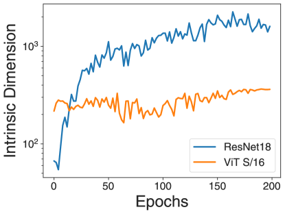
Figure 5: Non-linear intrinsic dimension $d_{nl}$ for models trained on MSE loss. For ResNet18 (blue), $d_{nl}$ increases by a factor of $10$ over training, while for ViT S/16 (orange) $d_{nl}$ remains relatively constant.

Appendix D Some examples of $\mu$ and $\nu$

In this section we give some examples of $\mu$ and $\nu$ as defined in equation (7) under various common distributions. First, we will describe how to define $\mu_{c}$ and $\nu_{c}$ as functions of the risk.

Notice that, with Gaussian data, $\ell_{\bm{\theta}}\overset{\operatorname{law}}{=}\sqrt{2\mathcal{R}(\bm{\theta})}\xi-\epsilon$ where $\xi$ is a standard Gaussian. Thus we can define $\tilde{\mu}$ and $\tilde{\nu}$ such that

$$\tilde{\mu}(\bm{\Theta}_{t})=\frac{\|\mathbb{E}[\operatorname{clip}_{c}(\sqrt{2\mathcal{R}(\bm{\Theta}_{t})}\xi-\epsilon)\mathbf{x}]\|}{\|\mathbb{E}[(\sqrt{2\mathcal{R}(\bm{\Theta}_{t})}\xi-\epsilon)\mathbf{x}]\|} \tilde{\nu}(\bm{\Theta}_{t})=\frac{\mathbb{E}[\operatorname{clip}^{2}_{c}(\sqrt{2\mathcal{R}(\bm{\Theta}_{t})}\xi-\epsilon)]}{\mathbb{E}[(\sqrt{2\mathcal{R}(\bm{\Theta}_{t})}\xi-\epsilon)^{2}]}$$ (156)

and $\mu_{c}(\bm{\Theta}_{t})=\tilde{\mu}_{c}(\mathcal{R}(\bm{\Theta}_{t}))$ and $\nu_{c}(\bm{\Theta}_{t})=\tilde{\nu}_{c}(\mathcal{R}(\bm{\Theta}_{t}))$. In what follows $r=\mathcal{R}(\bm{\theta})$ for some $\bm{\Theta}_{t}$. In the following examples, we will simplify notation and simply let $\mathcal{R}(\bm{\Theta}_{t})=r$.

D.1 Gaussian data and Gaussian noise

Consider $a\sim N(0,\mathbf{K})$ and $\epsilon\sim N(0,\sigma^{2})$. First define

$$F(z)=\operatorname{erf}\left(\frac{z}{\sqrt{2}}\right)-\sqrt{\frac{2}{\pi}}ze^{-z^{2}/2}$$ (157)

Then, we have

$$\mu_{c}(r)=\operatorname{erf}\left(\frac{c}{\sqrt{4(r+\sigma^{2}/2)}}\right)$$ (158)

$$(2r+\sigma^{2})\nu_{c}(r)=2rF\left(\frac{c}{\sqrt{2(r+\eta^{2}/2)}}\right)+c^{2}\operatorname{erfc}\left(\frac{c}{\sqrt{4(r+\eta^{2}/2)}}\right)$$ (159)

D.2 Gaussian data and Rademacher-like noise

$$\epsilon_{k}=\begin{cases}-\lambda&\text{with probability }q/2\\ 0&\text{with probability }1-q\\ \lambda&\text{with probability }q/2\end{cases}$$ (160)

Note that $\sigma^{2}=\operatorname{Var}(\epsilon)=\lambda^{2}q$. For some standard Gaussian random variable $z$, $\mu$ and $\nu$ may be computed as

$$\mu_{c}(r) =q\mathbb{P}\left(|z-\lambda|\leq\frac{c}{\sqrt{2r}}\right)+(1-q)\mathbb{P}\left(|z|\leq\frac{c}{\sqrt{2r}}\right)$$ (161)

$$=\frac{q}{2}\left(\operatorname{erf}\left(\frac{c-\lambda}{\sqrt{4r}}\right)+\operatorname{erf}\left(\frac{c+\lambda}{\sqrt{4r}}\right)\right)+(1-q)\operatorname{erf}\left(\frac{c}{\sqrt{4r}}\right)$$ (162)

$$(2r+\sigma^{2})\nu_{c}(r) =2r\frac{q}{2}\left(F\left(\frac{c-\lambda}{\sqrt{2r}}\right)+F\left(\frac{c+\lambda}{\sqrt{2r}}\right)\right)+2r(1-q)F\left(\frac{c}{\sqrt{2r}}\right)$$ (163)

$$+\frac{q\lambda}{\sqrt{\pi r}}\left(\exp\left(-\frac{(c+\lambda)^{2}}{2r}\right)-\exp\left(-\frac{(c-\lambda)^{2}}{2r}\right)\right)$$ (164)

$$+\frac{q\lambda^{2}}{2}\left(\operatorname{erf}\left(\frac{c-\lambda}{\sqrt{4r}}\right)+\operatorname{erf}\left(\frac{c+\lambda}{\sqrt{4r}}\right)\right)$$ (165)

$$+\frac{qc^{2}}{2}\left(\operatorname{erfc}\left(\frac{c-\lambda}{\sqrt{2r}}\right)+\operatorname{erfc}\left(\frac{c+\lambda}{\sqrt{2r}}\right)+(1-q)\mathbb{P}\left(|z|>\frac{c}{\sqrt{2r}}\right)\right)$$ (166)

D.3 Gaussian data and uniform noise

For $a\sim N(0,\mathbf{K})$ and uniform noise supported on $[-M,M]$ we have $\sigma^{2}=M^{2}/3$ and

$$\mu_{c}(r) =1-\frac{1}{2M}c^{2}\left(e^{-\frac{(c+M)^{2}}{4r}}(e^{\frac{cM}{r}}-1)\sqrt{\frac{4r}{\pi}}\right)$$ (167)

$$-\frac{1}{2M}c^{2}\left((M-c)\operatorname{erfc}\left(\frac{c-M}{\sqrt{4r}}\right)+(c+M)\operatorname{erfc}\left(\frac{c+M}{\sqrt{4r}}\right)\right)$$ (168)

$$(2r+\sigma^{2})\nu_{c}(r) =\frac{-1}{6M}e^{-\frac{(c+M)^{2}}{4r}}\sqrt{\frac{4r}{\pi}}\left(-c^{2}+cM-M^{2}-4r+e^{cM/r}(c^{2}+cM+M^{2}+4r)\right)$$ (169)

$$-\frac{1}{6M}(c^{3}-M^{3}-6Mr)\operatorname{erf}\left(\frac{c-M}{\sqrt{4r}}\right)+\frac{1}{6M}(c^{3}+M^{3}+6Mr)\operatorname{erf}\left(\frac{c+M}{\sqrt{4r}}\right)$$ (170)

$$+\frac{1}{2M}c^{2}\left(e^{-\frac{(c+M)^{2}}{4r}}(e^{\frac{cM}{r}}-1)\sqrt{\frac{2\sigma^{2}}{\pi}}\right)$$ (171)

$$+\frac{1}{2M}c^{2}\left((M-c)\operatorname{erfc}\left(\frac{c-M}{\sqrt{4r}}\right)+(c+M)\operatorname{erfc}\left(\frac{c+M}{\sqrt{4r}}\right)\right)$$ (172)

D.4 Gaussian data and symmetric exponential noise

For $a\sim N(0,\mathbf{K})$ and symmetric exponential noise, also known as Laplacian, with density

$$f(x)=\lambda e^{-|x|\lambda}/2$$ (173)

then we have

$$\mu_{c}(r) =2\operatorname{erf}\left(\frac{c}{\sqrt{2r^{2}}}\right)$$ (174)

$$+e^{\lambda(-2c+\lambda r^{2})/2}(e^{2c\lambda}-\operatorname{erf}\left(\frac{(c-\lambda r^{2})}{\sqrt{2r^{2}}}\right)-e^{2c\lambda}\operatorname{erf}\left(\frac{(c+\lambda r^{2})}{\sqrt{2r^{2}}}\right)-1)/2$$ (175)

Then, if $T_{c}(r)$ satisfies

$$(8+4\lambda^{2}r^{2})T(r) =2e^{\lambda(2c+\lambda r^{2})/2}(2-2c\lambda+c^{2}\lambda^{2})-2e^{\lambda(-2c+\lambda r^{2})/2}(2+2c\lambda+c^{2}\lambda^{2})$$ (176)

$$-4ce^{\frac{-c^{2}}{2r^{2}}}\lambda^{2}\sqrt{2r^{2}/\pi}+2\lambda^{2}r^{2}+2\lambda^{2}r^{2}(\operatorname{erf}\left(\frac{c}{\sqrt{2r^{2}}}\right)-1)$$ (177)

$$+(4+2\lambda^{2}r^{2}+8)\operatorname{erf}\left(\frac{c}{\sqrt{2r^{2}}}\right)$$ (178)

$$-2e^{\lambda(-2c+\lambda r^{2})/2}(2+2c\lambda+c^{2}\lambda^{2})\operatorname{erf}\left(\frac{c-\lambda r^{2}}{\sqrt{2r^{2}}}\right)$$ (179)

$$-2e^{\lambda(2c+\lambda r^{2})/2}(2-2c\lambda+c^{2}\lambda^{2})\operatorname{erf}\left(\frac{c+\lambda r^{2}}{\sqrt{2r^{2}}}\right)$$ (180)

we have

$$\nu_{c}(r)=T_{c}(r)+c^{2}(1-\mu_{c}(r))/(2r+\sigma^{2})$$ (181)

Appendix E Proof of stability and effectiveness theorems

E.1 Proof of Theorem 2

To see there exists $c>0$ such that (CSC) holds, it is simpler to work with the inverse of the ratio. We remark that

$$\lim_{c\to 0^{+}}\frac{\nu_{c}}{\mu_{c}} =\lim_{c\to 0^{+}}\frac{\mathbb{E}(\ell^{2}\mathbbm{1}_{|\ell|\leq c}+c^{2}\mathbbm{1}_{|\ell|>c})}{\mathbb{P}(|\ell|\leq c)}$$ (182)

$$=\lim_{c\to 0^{+}}\frac{1}{{\mathbb{P}(|\ell|\leq c)}}\int_{|\ell|\leq c}\ell^{2}\,d\mathbb{P}+\frac{c^{2}(1-\mathbb{P}(|\ell|\leq c))}{\mathbb{P}(|\ell|\leq c)}$$ (183)

$$=\lim_{c\to 0^{+}}\frac{1}{{\mathbb{P}(|\ell|\leq c)}}\int_{|\ell|\leq c}\ell^{2}\,d\mathbb{P}+\frac{c^{2}}{\mathbb{P}(|\ell|<c)}.$$ (184)

Therefore, it suffices to show that (184) is less than $1$. Indeed, the former term converges to $0$ by the Lebesgue-Differentiation Theorem. For the latter, let us assume that $\epsilon\sim\pi$ for some probability-measure $\pi$. Given that $\mathbf{x}\sim N(0,\mathbf{K})$, let us denote $f$ to be the (Gaussian) density of $\left\langle\mathbf{x},\bm{\theta}-{\bm{\theta}^{*}}\right\rangle$. It follows that

$$\mathbb{P}(|\ell|\leq c) =\mathbb{P}(-c+\epsilon\leq\left\langle\mathbf{x},\bm{\theta}-\bm{\theta}^{*}\right\rangle\leq c+\epsilon)$$ (185)

$$=\int_{\mathbb{R}}\int_{-c+\epsilon}^{c+\epsilon}f(x)\,dx\,d\pi(\epsilon).$$ (186)

Differentiating with respect to $c$ yields,

$$\frac{d}{dc}\left(\int_{\mathbb{R}}\int_{-c+\epsilon}^{c+\epsilon}f(x)\,dx\,d\pi(\epsilon)\right)=\int_{\mathbb{R}}f(c+\epsilon)+f(-c+\epsilon)\,d\pi(\epsilon).$$ (187)

By L’Hôpital’s rule, the latter term of (184) becomes

$$\lim_{c\to 0}\frac{c^{2}}{\mathbb{P}(|\ell|<c)} =\lim_{c\to 0}\frac{2c}{\int_{\mathbb{R}}f(c+\epsilon)+f(-c+\epsilon)\,d\pi(\epsilon)}$$ (188)

$$=\lim_{c\to 0^{+}}\frac{2c}{\int_{\mathbb{R}}2f(\epsilon)\,d\pi(\epsilon)}$$ (189)

$$=0.$$ (190)

E.2 Proof of Theorem 3

First, notice that $\sigma^{2}=q\lambda^{2}$. In the limit as $|R_{t}|\to 0$ we have,

$$\mu(R_{t}) =\mathbb{P}(|\epsilon|\leq c)$$ (191)

$$=\begin{cases}1&\lambda\leq c\\ 1-q&\lambda>c\end{cases}$$ (192)

$$\nu(R_{t})=\begin{cases}1&\lambda\leq c\\ c^{2}/\lambda^{2}&\lambda>c\end{cases}$$ (193)

thus

$$\frac{\mu(R_{t})}{\nu(R_{t})} =1 \lambda<c$$ (194)

$$\frac{\mu(R_{t})}{\nu(R_{t})} >1 c<\sqrt{(1-q)}\lambda$$ (195)

$$\frac{\mu(R_{t})}{\nu(R_{t})} \leq 1 \sqrt{(1-q)}\lambda\leq c<\lambda$$ (196)

thus $c$ may always be chosen such that the (CSC) is less than $1$.

E.3 Proof of Theorem 5

With $\mu$ and $\nu$ given by equations (158) and (159) we have that

$$\lim_{c\to 0}\frac{\mu^{2}(R_{t})}{\nu(R_{t})}=\frac{2}{\pi}<1$$ (197)

Meanwhile, it can be seen that for all $R_{t}\geq 0$ $\mu^{2}_{c}(R_{t})/\nu_{c}(R_{t})$ is increasing and continuous in $c$. Since,

$$\lim_{c\to\infty}\frac{\mu_{c}^{2}(R_{t})}{\nu(R_{t})}=1$$ (198)

we are done.

E.4 Proof of Theorem 6

In light of Section E.2 above, we see that

$$\frac{\mu_{c}(R_{t})^{2}}{\nu_{c}(R_{t})} =1 \lambda<c$$ (199)

$$\frac{\mu_{c}(R_{t})^{2}}{\nu_{c}(R_{t})} >1 c<(1-q)\lambda$$ (200)

$$\frac{\mu_{c}(R_{t})^{2}}{\nu_{c}(R_{t})} \leq 1 (1-q)\lambda\leq c<\lambda$$ (201)

thus $c$ may always be chosen such that the (CCC) holds.

Appendix F The risk under anisotropic data

In this section, we describe how to use equation (12) to solve for the risk. Using Itô’s Lemma and the resolvent identity $R(z;\mathbf{K})(\mathbf{K}-z)=\mathbf{I}$.

$$\mathrm{d}q_{z}(\bm{\Theta}_{t})= -\eta(t)\left(\|\bm{\Theta}_{t}-{\bm{\theta}^{*}}\|^{2}+2zq_{z}(\bm{\Theta}_{t})\right)\mu_{c(t)}(\mathcal{R}(\bm{\Theta}_{t}))\mathrm{d}t$$ (202)

$$+\frac{\eta^{2}(t)}{d}\operatorname{Tr}(\mathbf{K}R(z;\mathbf{K}))\nu_{c(t)}(\mathcal{R}(\bm{\Theta}_{t}))\mathrm{d}t+\mathrm{d}\mathcal{M}_{t}.$$

We shall let $Q_{z}(t)$ be the deterministic equivalent of this equation, that is

$$\frac{\mathrm{d}}{\mathrm{d}t}Q_{z}(t)=-\eta(t)\left(\mathcal{D}_{t}+2zQ_{z}(t)\right)\mu_{c(t)}(R_{t})+\frac{\eta^{2}(t)}{d}\operatorname{Tr}(\mathbf{K}R(z;\mathbf{K}))\nu_{c(t)}(R_{t}),$$ (203)

where (recalling $\Omega$ is the circle of radius $2$)

$$D_{t}=\frac{-1}{2\pi i}\oint_{\Omega}Q_{z}(t)\mathrm{d}z\quad\text{and}\quad R_{t}=\frac{-1}{2\pi i}\oint_{\Omega}zQ_{z}(t)\mathrm{d}z.$$

These are analogues of the same formulas that hold exactly for $\mathcal{D}(\bm{\Theta}_{t})$ and $\mathcal{R}(\bm{\Theta}_{t})$ when replacing $Q_{z}$ by $q_{z}(\bm{\Theta}_{t})$.

Now it is possible to precisely compare the solution of these ODEs to SGD, as the same machinery developed for Theorem 1 applies. In particular, Lemma 1 bounds the supremum difference $\sup_{z\in\Omega}|q_{z}(\Theta_{t})-Q_{z}(t)|$ (although now with $\mathcal{M}_{t}^{SDE}\equiv 0$). Hence, we conclude the following:

Theorem 8.

Suppose that Assumptions 1, 2 and 3 hold. Suppose that $\{\bm{\theta}_{k}\}$ is C-SGD. Let $\overline{c}=\sup_{t}c(t)$ and ${\overline{\eta}}=\sup_{t}{\eta}(t)$. There is a constant $\mathcal{C}=\mathcal{C}(\dutchcal{v},(n/d),\overline{c},\overline{\eta},\|\bm{\theta}_{0}-{\bm{\theta}^{*}}\|^{2})$, a stochastic process $\mathcal{E}$, and a constant $m=m(\dutchcal{v})$ so that for any $1\leq u\leq md$

$$\sup_{0\leq k\leq n}\left\|\begin{bmatrix}\mathcal{R}(\bm{\theta}_{k})\\ \mathcal{D}(\bm{\theta}_{k})\end{bmatrix}-\begin{bmatrix}R_{k/d}\\ D_{k/d}\end{bmatrix}\right\|\leq\mathcal{C}\mathcal{E}(n/d)u\log(d)d^{-1/2},$$ (204)

with probability $1-e^{-u}$ and provided the right hand side is less than $1$. The stochastic process $\mathcal{E}$ is given by

$$\mathcal{E}(t)=\exp\left(\int_{0}^{t}\frac{C{\eta}(s)^{2}\sigma\,\mathrm{d}s}{\sqrt{\mathcal{R}(\bm{\Theta}_{s})+R_{s}}}\right)$$

for an absolute constant $C>0$. The constant $\mathcal{C}$ can be bounded by

$$\mathcal{C}\leq C\sqrt{n/d}\,\overline{\eta}\dutchcal{v}^{2}\cdot((1+\|\bm{\theta}_{0}-{\bm{\theta}^{*}}\|^{2})\dutchcal{v}^{2}+\overline{c}^{2}\sqrt{n/d})\cdot\exp\left(C\max\{\overline{\eta},\overline{\eta}^{2}\}(n/d)\right)$$

for an absolute constant $C>0.$

We note that further details in this direction are shown in [19].

F.1 Getting a system of ODEs

We may use Equation (203) to get an equivalent coupled system of $\dutchcal{d}$ ODEs which can solve for $R_{t}$. First, we may diagonalize,

$$\mathbf{K}=\sum_{i=1}{d}\lambda_{i}w_{i}w_{i}^{T} R(z;\mathbf{K})=\sum_{i=1}{d}\frac{1}{\lambda_{i}-z}w_{i}w_{i}^{T}$$ (205)

Where $\{\lambda_{i}\}_{i=1}{d}$ and $\{w_{i}\}_{i=1}{d}$ are the eigenvalues and eigenvectors of $\mathbf{K}$ respectively. Therefore,

$$Q_{z}(\bm{\Theta}_{t})=\frac{1}{2}\sum_{i=1}{d}\frac{1}{\lambda_{i}-z}\left\langle\bm{\Theta}_{t}-{\bm{\theta}^{*}},w_{i}\right\rangle^{2}.$$ (206)

Define $v_{i}(t)=\left\langle\bm{\Theta}_{t}-{\bm{\theta}^{*}},w_{i}\right\rangle^{2}/2$. Then, $R_{t}=\sum_{i=1}{d}v_{i}(t)\lambda_{i}$ and $D_{t}=\sum_{i=1}{d}2v_{i}(t)$. Now, we can find a system of ODEs which describes the evolution of $\{v_{i}\}_{i=1}{d}$.

Choose $\Omega_{i}$ to be a complex curve enclosing only the $i$-th eigenvalue of $\mathbf{K}$. Integrating over both sides of equation (203) and using Cauchy’s integral formula, we see that

$$\frac{\mathrm{d}v_{i}}{\mathrm{d}t}=-2\eta(t)v_{i}\lambda_{i}\mu_{c(t)}(R_{t})+\frac{\eta(t)^{2}}{d}\lambda_{i}\nu_{c(t)}(R_{t})(R_{t}+\sigma^{2}/2),\quad\forall i\in[\dutchcal{d}].$$ (207)

This final system of ODEs is used in all experiments to solve for $R_{t}$.

F.2 Getting an Integral Equation

Here we follow techniques of existing theory [20]. Using Equation (203) and an integrating factor we see that

$$Q_{z}(t)= Q_{z}(0)e^{-2z\Omega_{t}^{c}}+\frac{1}{d}\int_{0}^{t}\eta(s)^{2}\nu_{c(s)}(R_{s})\operatorname{Tr}(\mathbf{K}R(z;\mathbf{K})e^{-2z(\Omega_{t}^{c}-\Omega_{s}^{t})})(R_{s}+\sigma^{2}/2)\mathrm{d}s$$ (208)

$$-\eta(t)D_{t}e^{-2z\Omega_{t}^{c}}\mu_{c(t)}(R_{t})$$

where $\Omega_{t}^{c}=\int_{0}^{t}\eta(s)\mu_{c(s)}(R_{s})\mathrm{d}s$ is the integrated clipped learning rate. Now, multiplying by $z$, integrating both sides around $\Omega$, and multiplying by $-1/2\pi i$, we get

$$R_{t}=\mathcal{R}(\bm{\Phi}^{\mathrm{gf}}_{\Gamma_{T}^{c}})+\frac{1}{d}\int_{0}^{t}{\tilde{\eta}}^{2}(s)\nu_{c_{s}}\operatorname{Tr}(\mathbf{K}^{2}e^{-2\mathbf{K}(\Gamma_{t}^{c}-\Gamma_{s}^{c})})(R_{s}+\sigma^{2}/2)\mathrm{d}s,$$ (209)

where the first term is identified with gradient flow as in [20].

Appendix G Experimental details

G.1 Clipped SGD and Homogenized Clipped SGD

The experiments creating Figure 1 were carried out on a standard Google Colab CPU runtime. Homogenized clipped SGD is solved via a standard Euler-Maruyama algorithm. The procedure for solving for the risk is described in Appendix F.

The experiments creating Figure 4 were again carried out on a standard Google Colab CPU runtime. Numerical optimization of the max-(CCC) clipping schedule (Equation (19)) was done via the Nelder-Mead algorithm using standard python libraries.

The code to reproduce these results, including all plots of stability thresholds (Figure 2, and Figure 3), is supplied in the Supplementary Materials.

G.2 Intrinsic dimension experiments

The experiments in Appendix C were carried out on $8$ P100 GPUs trained in parallel with batch size $128$. This allowed for efficient computation of the full batch Gauss-Newton operator norm via power iteration. Both networks were trained for $200$ epochs. ResNet18 was trained with cosine learning rate decay (base learning rate $0.05$), while ViT was trained with linear warmup for $2$ epochs followed by a cosine learning rate decay (base learning rate $0.00625$). Both networks used GELU activation function.

References

- [1] Tomáš Mikolov “Statistical Language Models based on Neural Networks”, 2012
- [2] Razvan Pascanu, Tomáš Mikolov and Yoshua Bengio “On the difficulty of training recurrent neural networks” In Proceedings of the 30th International Conference on Machine Learning, 2013
- [3] Tom Brown et al. “Language Models are Few-Shot Learners” In Advances in Neural Information Processing Systems 33 Curran Associates, Inc., 2020, pp. 1877–1901 URL: https://proceedings.neurips.cc/paper_files/paper/2020/file/1457c0d6bfcb4967418bfb8ac142f64a-Paper.pdf
- [4] Martin Abadi et al. “Deep Learning with Differential Privacy” In Proceedings of the 2016 ACM SIGSAC Conference on Computer and Communications Security ACM, 2016
- [5] Venkatadheeraj Pichapati et al. “AdaCliP: Adaptive Clipping for Private SGD”, 2019 arXiv:1908.07643 [cs.LG]
- [6] Ilya O Tolstikhin et al. “MLP-Mixer: An all-MLP Architecture for Vision” In Advances in Neural Information Processing Systems 34, 2021, pp. 24261–24272
- [7] Alexey Dosovitskiy et al. “An Image is Worth 16x16 Words: Transformers for Image Recognition at Scale” In International Conference on Learning Representations, 2021
- [8] Jingzhao Zhang et al. “Why are Adaptive Methods Good for Attention Models?” In Advances in Neural Information Processing Systems 33 Curran Associates, Inc., 2020, pp. 15383–15393
- [9] Jared Kaplan et al. “Scaling Laws for Neural Language Models”, 2020 arXiv:2001.08361 [cs.LG]
- [10] Kaiming He, X. Zhang, Shaoqing Ren and Jian Sun “Deep Residual Learning for Image Recognition” In 2016 IEEE Conference on Computer Vision and Pattern Recognition (CVPR), 2015, pp. 770–778 URL: https://api.semanticscholar.org/CorpusID:206594692
- [11] Jia Deng et al. “ImageNet: A large-scale hierarchical image database” In 2009 IEEE Conference on Computer Vision and Pattern Recognition, 2009, pp. 248–255 DOI: 10.1109/CVPR.2009.5206848
- [12] Jacob Devlin, Ming-Wei Chang, Kenton Lee and Kristina Toutanova “BERT: Pre-training of Deep Bidirectional Transformers for Language Understanding” In North American Chapter of the Association for Computational Linguistics, 2019 URL: https://api.semanticscholar.org/CorpusID:52967399
- [13] Anastasia Koloskova, Hadrien Hendrikx and Sebastian U Stich “Revisiting Gradient Clipping: Stochastic bias and tight convergence guarantees” In Proceedings of the 40th International Conference on Machine Learning, 2023
- [14] Bohang Zhang, Jikai Jin, Cong Fang and Liwei Wang “Improved Analysis of Clipping Algorithms for Non-convex Optimization” In Advances in Neural Information Processing Systems, 2020
- [15] Xiangyi Chen, Steven Z. Wu and Mingyi Hong “Understanding Gradient Clipping in Private SGD: A Geometric Perspective” In Advances in Neural Information Processing Systems, 2020
- [16] Qianxiao Li, Cheng Tai and Weinan E “Stochastic Modified Equations and Adaptive Stochastic Gradient Algorithms” In Proceedings of the 34th International Conference on Machine Learning 70, Proceedings of Machine Learning Research PMLR, 2017, pp. 2101–2110
- [17] Stephan Mandt, Matthew D. Hoffman and David M. Blei “A Variational Analysis of Stochastic Gradient Algorithms”, 2016 arXiv:1602.02666 [stat.ML]
- [18] David Barrett and Benoit Dherin “Implicit Gradient Regularization” In International Conference on Learning Representations, 2021
- [19] Elizabeth Collins-Woodfin, Courtney Paquette, Elliot Paquette and Inbar Seroussi “Hitting the High-Dimensional Notes: An ODE for SGD learning dynamics on GLMs and multi-index models” In arXiv e-prints, 2023, pp. arXiv:2308.08977 DOI: 10.48550/arXiv.2308.08977
- [20] Courtney Paquette, Elliot Paquette, Ben Adlam and Jeffrey Pennington “Homogenization of SGD in high-dimensions: Exact dynamics and generalization properties”, 2022 arXiv:2205.07069 [math.ST]
- [21] Atish Agarwala, Fabian Pedregosa and Jeffrey Pennington “Second-order regression models exhibit progressive sharpening to the edge of stability” In Proceedings of the 40th International Conference on Machine Learning 202, Proceedings of Machine Learning Research PMLR, 2023, pp. 169–195 URL: https://proceedings.mlr.press/v202/agarwala23b.html
- [22] Jeremy Cohen et al. “Gradient Descent on Neural Networks Typically Occurs at the Edge of Stability” In International Conference on Learning Representations, 2021 URL: https://openreview.net/forum?id=jh-rTtvkGeM
- [23] Atish Agarwala and Jeffrey Pennington “High Dimensional Analysis Reveals Conservative Sharpening and a Stochastic Edge of Stability” arXiv, 2024 DOI: 10.48550/arXiv.2404.19261
- [24] Roman Vershynin “High-Dimensional Probability: An Introduction with Applications in Data Science”, Cambridge Series in Statistical and Probabilistic Mathematics Cambridge University Press, 2018
- [25] Elizabeth Collins-Woodfin and Elliot Paquette “High-dimensional limit of one-pass SGD on least squares”, 2023 arXiv:2304.06847 [math.PR]
- [26] Kaiming He, Xiangyu Zhang, Shaoqing Ren and Jian Sun “Deep Residual Learning for Image Recognition” In Proceedings of the IEEE Conference on Computer Vision and Pattern Recognition, 2016, pp. 770–778
- [27] Alexey Dosovitskiy et al. “An image is worth 16x16 words: Transformers for image recognition at scale” In arXiv preprint arXiv:2010.11929, 2020