CHG Shapley: Efficient Data Valuation and Selection towards Trustworthy Machine Learning
Abstract
Understanding the decision-making process of machine learning models is crucial for ensuring trustworthy machine learning. Data Shapley, a landmark study on data valuation, advances this understanding by assessing the contribution of each datum to model accuracy. However, the resource-intensive and time-consuming nature of multiple model retraining poses challenges for applying Data Shapley to large datasets. To address this, we propose the CHG (Conduct of Hardness and Gradient) score, which approximates the utility of each data subset on model accuracy during a single model training. By deriving the closed-form expression of the Shapley value for each data point under the CHG score utility function, we reduce the computational complexity to the equivalent of a single model retraining, an exponential improvement over existing methods. Additionally, we employ CHG Shapley for real-time data selection, demonstrating its effectiveness in identifying high-value and noisy data. CHG Shapley facilitates trustworthy model training through efficient data valuation, introducing a novel data-centric perspective on trustworthy machine learning.
1 Introduction
The central problem of trustworthy machine learning is explaining the decision-making process of models to enhance the transparency of data-driven algorithms. However, the high complexity of machine learning model training and inference processes obscures an intuitive understanding of their internal mechanisms. Approaching trustworthy machine learning from a data-centric perspective (Liu et al., 2023) offers a new perspective for research. For trustworthy model inference, a representative algorithm is the SHAP (Lundberg and Lee, 2017), which quantitatively attributes model outputs to input features, clarifying which features influence specific results the most. SHAP and its variants(Kwon and Zou, 2022b) are widely applied in data analysis and healthcare. For trustworthy model training, the Data Shapley algorithm (Ghorbani and Zou, 2019) stands out. It quantitatively attributes a model’s performance to each training data point, identifying valuable data that improves performance and noisy data that degrades it. Data valuation not only informs us about the extent to which each training data impacts model performance but also underpins subsequent tasks such as data selection, data acquisition, data cleaning, etc., and supports the development of data markets (Mazumder et al., 2023).
The impressive effectiveness of both SHAP and Data Shapley algorithms is rooted in the Shapley value (Shapley, 1953). The unique feature of the Shapley value lies in its ability to accurately and fairly allocate contributions to each factor in decision-making processes where multiple factors interact with each other. However, the exact computation of the Shapley value is , where is the number of participants. Consequently, even when employing estimation methods akin to linear least squares regression (Lundberg and Lee, 2017) or Monte Carlo (Ghorbani and Zou, 2019), the efficiency of SHAP and Data Shapley algorithms sometimes fails to meet requirements. For example, the most efficient known data valuation method is KNNShapley (Jia et al., 2019) designed for the k-nearest neighbors algorithm, requiring times of model retraining, where is the number of training data.
In this paper, we focus on the efficiency problem of data valuation on large-scale datasets. Instead of investigating more efficient and robust algorithms to approximate the Shapley value like in (Lundberg and Lee, 2017; Wang and Jia, 2023; Wang et al., 2024b), we concentrate on estimating the utility function. The underlying idea is that if the accuracy estimation function of a model trained on a subset can be analytically expressed through some features of the subset, then it becomes possible to directly derive an analytic expression for the Shapley value of each data point.
Our contributions are summarized as follows:
Efficient and Large-Scale Data Valuation Method: We introduce the CHG (Conduct of Hardness and Gradient) score, which assesses the influence of a data subset on model accuracy. By deriving the analytical expression for the Shapley value of each data point under this utility function, we significantly improve upon the time complexity of Data Shapley. Using our proposed CHG Shapley method, valuing the full training dataset takes at most twice the time of conventional training, equivalent to one additional model retraining.
Real-Time Selection of Training Data in Large-Scale Datasets Based on Data Valuation: We employ CHG Shapley for real-time data selection. Experiments involving data-efficient training and model training under noise labels demonstrate the effectiveness of CHG Shapley in identifying high-value and noisy data.
A New Data-Centric Perspective on Trustworthy Machine Learning: CHG Shapley is a parameter-free method, deriving its benefits solely from a deeper understanding of the data. We believe that approaches rooted in data valuation have the potential to enhance understanding of model mechanisms, thereby advancing trustworthy machine learning.
2 Background and Related Works
Data-centric AI. For an extended period, the machine learning research community has predominantly concentrated on model development rather than on the underlying datasets (Mazumder et al., 2023). However, the inaccuracies, unfairness, and biases in models caused by data have become increasingly severe in real-world applications (Wang et al., 2023). Conducting trustworthy machine learning research from a data-centric perspective has garnered increasing attention from researchers (Liu et al., 2023). Research on data valuation can also be seen as an effort to understand the machine learning model training process from a data-centric perspective.
Shapley value. Supposing some players cooperate to finish a task, we denote the player set as and the utility function defined on every subset of is denoted as , then the Shapley value (Shapley, 1953) is the unique solution concept that satisfies the following four axioms:
-
•
Dummy player: If for all , then .
-
•
Symmetry: If for all , then .
-
•
Linearity: For utility functions and any , .
-
•
Efficiency: .
Definition 1 (Shapley (1953))
Given a player set and a utility function , the Shapley value of a player is defined as
| (1) |
Data valuation. Data valuation aims to quantitatively analyze the impact of training data on the performance of machine learning models, particularly deep neural networks. Determining the value of data can facilitate tasks such as data selection (Wang et al., 2024c), acquisition(Mazumder et al., 2023), and trading(Wang et al., 2024a). Since the performance of machine learning models is derived from the collective contribution of all data points, a fair data valuation algorithm is essential to accurately attribute each data point’s contribution to the model’s performance.
A milestone in data valuation research is the Data Shapley algorithm developed by Ghorbani and Zou (2019). Data Shapley builds upon the Shapley value formula by treating all data in the training dataset as players in a cooperative game of "training the model together". represents the accuracy achieved by training the model on dataset subset . Consequently, the Shapley value computed for each data point serves as an indication of its contribution to model performance. Data points with lower values are considered more likely to be harmful, while those with higher values are deemed to be lacking in the model’s representation. Removing low-value data points or acquiring more high-value data points can lead to improved model accuracy, a hypothesis supported by related experiments. Following Data Shapley, several subsequent have been proposed.
KNN Shapley(Jia et al., 2019) focus on the Shapley value of the k-nearest neighbors algorithm, proposing the closed-form expression of the Shapley value of the KNN scenario, notably improving computational efficiency to .
Beta Shapley (Kwon and Zou, 2022a) was developed to address an issue identified in Data Shapley regarding the uniform weight allocation for sets with different cardinalities. By relaxing the efficiency axiom in the Shapley value and utilizing a beta distribution to characterize the weights of sets of different cardinalities, Beta Shapley performs better than Data Shapley in tasks such as detecting mislabeled training data.
Data Banzhaf (Wang and Jia, 2023) aims to mitigate the noise introduced by stochastic gradient algorithms on model accuracy (i.e., utility function) during the model training process. Banzhaf value has also been demonstrated to be the most robust solution concept among all semi-values (i.e., Shapley values without Efficiency restrictions) in the presence of noise in the utility function. Therefore, Data Banzhaf is well-suited for evaluating training data in deep learning scenarios.
Additionally, there has been a surge in work on machine learning systems that utilize Shapley values to compute data values (Karlaš et al., 2024). All these studies utilize the Shapley value or its variants as their theoretical foundation because it is widely acknowledged in cooperative game theory as the fairest method for allocating contributions (Algaba et al., 2019).
To provide a more detailed assessment of various data valuation algorithms, Jiang et al. (2023) introduced the OpenDataVal benchmark library. This benchmark library abstracts away details such as model training, allowing researchers to focus solely on algorithm design for data valuation. We also use this benchmark to evaluate our proposed data valuation algorithm.
3 Efficient Data valuation
"What’s the value of your data?" Instead of directly assessing the contribution of each data point to model accuracy, we initially explore another pertinent question: "Which data holds greater value in the training process?" In the realm of data selection, numerous significant studies offer varying perspectives. Some focus on the utility of individual data, employing methods such as influence functions (Koh and Liang, 2017; Yang et al., 2023; Chhabra et al., 2024), EL2N score (Paul et al., 2021), InfoBatch (Qin et al., 2024), and worst-case training methods (Huang et al., 2022). These approaches utilize data information and model parameters to calculate a score (e.g., loss) for data selection. Conversely, another approach emphasizes the utility of data subsets (Killamsetty et al., 2021a, b; Zhao et al., 2021), aiming to identify representative subsets of the original dataset that can achieve comparable model accuracy, often utilizing corresponding gradient subsets. We reconcile these two perspectives and introduce the CHG score as a measure of data subset accuracy.
3.1 Preliminaries
Let denotes a labeled training set. The objective is to assign a scalar to each training data point based on its contribution to the model’s performance. A utility function , mapping from any subset of the training set (including the empty set) to the performance of the model trained on the subset (denoted as ), is usually used for data valuation. In Data Shaply(Ghorbani and Zou, 2019), the accuracy of the model on a hold-out test set is used as .
3.2 CHG Score as a Utility Function for Subset Model Performance
The opacity of , or the fact that can only be obtained after training a model on , renders marginal contribution-based data valuation algorithms such as Data Shapley (Ghorbani and Zou, 2019), Beta Shapley (Kwon and Zou, 2022a), Data Banzhaf (Wang and Jia, 2023), AME (Lin et al., 2022), and LOO (leave-one-out error) time-consuming and computationally intensive.
On the contrary, if we can determine the model’s accuracy on without training on it, or even derive the expression for in terms of , then we can significantly reduce the model training time and expedite the calculation of each data’s value. To achieve this, we first investigate the impact of training the model using a subset of data .
Here we focus on the model training process. Assuming that in the current iteration, the model parameters are denoted by . We use to represent the loss function of the neural network across the entire training dataset. A smaller loss indicates higher model accuracy on the training dataset.
Assuming at this point, no overfitting has occurred, i.e., the model’s accuracy on the training and test datasets is comparable, we can reasonably utilize the training dataset’s loss to estimate the model’s accuracy on the test dataset. If we update the parameters by training on the subset using gradient descent, then the next update direction of the parameters is , where represents the gradient of the -th data point. After one step of gradient descent, becomes . Subsequently, based on the following lemma, can be considered as a metric for evaluating the model’s performance.
Lemma 1 ((Nesterov, 2018))
Let be any differentiable function with -Lipschitz continuous gradient, , and 111This is a commonly used assignment method, for example, in proving the convergence of gradient descent for non-convex functions to local minima (Nesterov, 2018), was set as , then we have:
| (2) |
Proof: The first inequality is due to the definition of -Lipschitz continuity.
When using traditional empirical risk minimization, measuring the model’s performance using the gradients of the training set on the training process is acceptable. However, inspired by the principles of worst-case training method (Huang et al., 2022) and InfoBatch (Qin et al., 2024), we introduce a method to incorporate the difficulty of data points into the model optimization process.
Specifically, our optimization objective is to minimize rather than (i.e., empirical risk minimization), where is equal to but does not participate in model backpropagation. can be viewed as the hardness of learning this data point. Generally, when there is no label noise, focusing on hard-to-learn data points can help improve the model’s generalization ability (Huang et al., 2022) and may reduce training time (Qin et al., 2024). Then the gradient of -th data changes from to , and then we define the Conduct of Hardness and Gradient score (CHG score) of a data subset as . We use this score to measure the influence of data subsets on model accuracy. We also investigate the performance of the Hardness score ( ) and Gradient Score ( ) in Table 2, see Hardness Shapley and Gradient Shapley.
| Algorithms | Underlying Method | Model Retraining Complexity | Quality of Data Values | |||
| Noisy Label | Noisy Feature | Point | Point | |||
| Detection | Detection | Removal | Addition | |||
| LOO | Marginal contribution | - | - | + | + | |
| Data Shapley (Ghorbani and Zou, 2019) | Marginal contribution | + | + | ++ | ++ | |
| KNN Shapley (Jia et al., 2019) | Marginal contribution | NA | + | + | ++ | ++ |
| Beta Shapley (Kwon and Zou, 2022a) | Marginal contribution | + | + | ++ | ++ | |
| Data Banzhaf (Wang and Jia, 2023) | Marginal contribution | - | - | + | + | |
| AME (Lin et al., 2022) | Marginal contribution | - | - | ++ | + | |
| Influence Function (Koh and Liang, 2017) | Gradient | NA | - | - | + | + |
| LAVA (Just et al., 2023) | Gradient | NA | - | ++ | + | + |
| DVRL (Yoon et al., 2020) | Importance weight | + | - | + | ++ | |
| Data-OOB (Kwon and Zou, 2023) | Out-of-bag estimate | NA | ++ | + | - | ++ |
| CHG Shapley (this paper) | Marginal contribution, | ++ | + | ++ | NA | |
| Gradient and Loss | ||||||
3.3 CHG Shapley
After obtaining the utility function (CHG score), which approximates the influence of data subsets on model accuracy using gradient and loss information during model training, we can derive the analytical expression for the Shapley value of each data point under this utility function. This enables efficient computation of the value of each data point in large-scale datasets.
Theorem 1
Supposing for any subset , , then the Shapley value of j-th data point can be expressed as:
| (3) | ||||
Proof see Appendix B
We implemented our CHG Shapley data valuation method (see Algorithm 1) based on the code foundation of OpenDataVal (Jiang et al., 2023) and conducted experiments on the CIFAR-10 embedding dataset on a NVIDIA A40 server. The model used is pre-trained ResNet50 + logistic regression, and we report the results in Table 1.
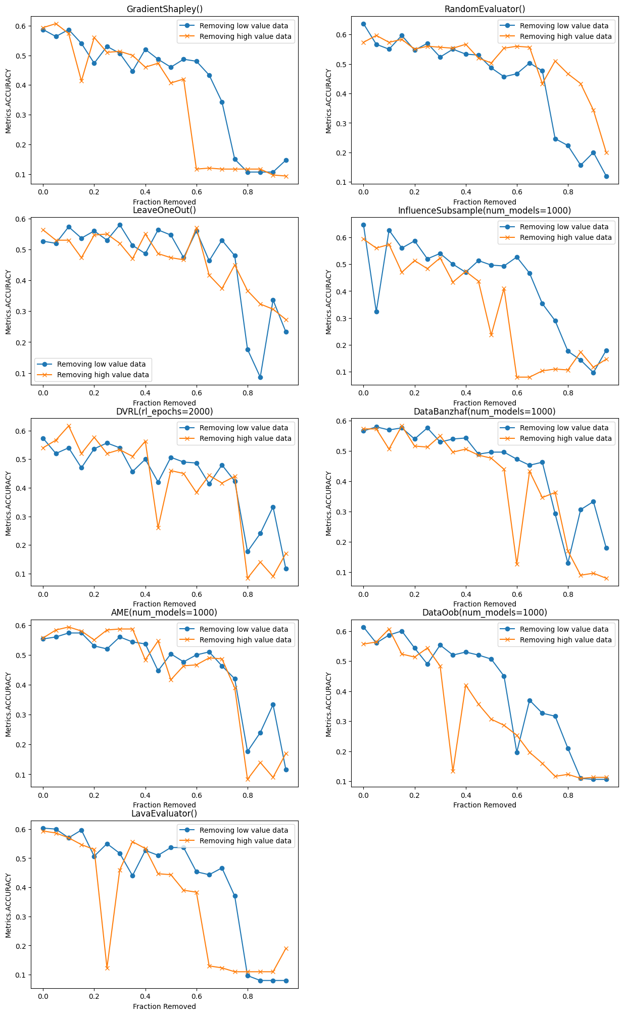
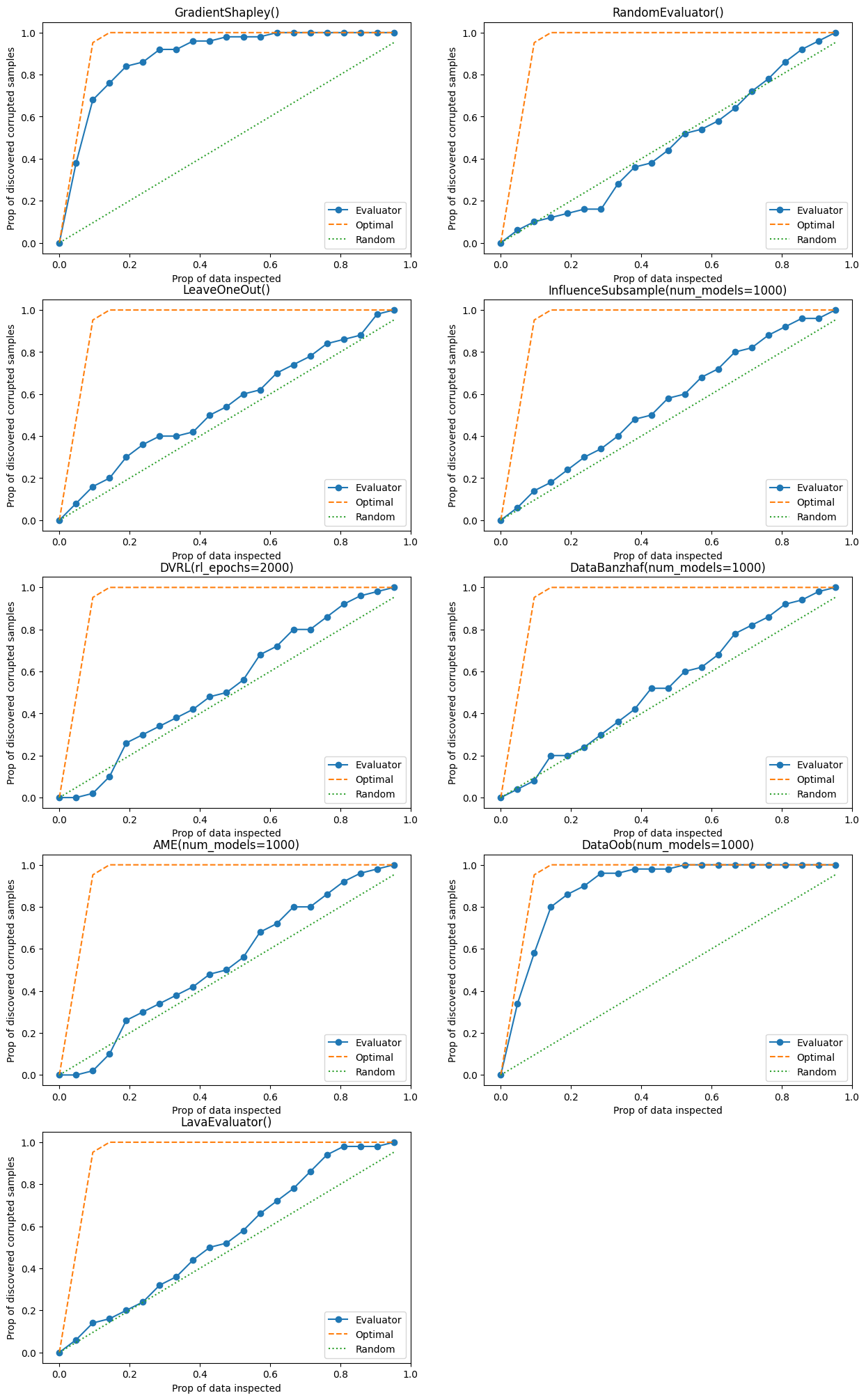
For noisy label detection tasks and comparisons with other data evaluation methods, see Picture 2. For point removal tasks, see Picture 1.
The experimental results demonstrate that CHG Shapley data valuation method not only exhibits excellent data valuation and noise data detection capabilities, but also achieves remarkable operational efficiency. This is made possible by our research into the utility function that measures the impact of data subsets on model accuracy. In the next section, we will further show its data selection ability based on data valuation and noise label detection.
4 Data Selection
In this section, we introduce various implementation strategies and practical techniques to enhance the scalability and efficiency of CHG Shapley. The experiments are conducted on a NVIDIA A40 server.
Last-Layer Gradients: Modern deep learning models possess a vast number of parameters, resulting in high-dimensional gradients. To mitigate this issue, we adopt a last-layer gradient approximation as in(Killamsetty et al., 2021a, b). This technique focuses solely on the gradients of the last layer for neural networks in CHG Shapley, significantly improving the speed of the algorithm and other baseline methods.
Per-Class Approximations: To enhance model performance, we adopt a per-class approach. This method involves caluclate the CHG Shapley separately for each class, which means considering only the data instances belonging to each class in each iteration. This approach not only reduces memory requirements but also decreases computational overhead, thereby improving the overall efficiency of the CHG Shapley-based data selection algorithm.
CHG Shapley-based Data Selection Algorithm: Here, we detail the CHG Shapley Data Selection Algorithm, integrating the aforementioned techniques to ensure efficient and scalable data valuation and selection.
Results: We report the accuracy and time consumption comparisons in Table 2 under the data pruning setting. CHG Shapley demonstrates particularly strong performance when the selection ratio is small, highlighting its ability to identify high-value data effectively. Additionally, the time consumption remains acceptable even when considering data selection processes, underscoring the high efficiency of CHG Shapley as a data valuation method. This efficiency, combined with its accuracy, verifies that CHG Shapley is a practical and powerful tool for data selection and valuation in large-scale machine learning tasks.
The results presented in Table 3, where 30% of the class labels were randomly replaced with other labels, provide additional evidence of CHG Shapley’s capability to detect mislabeled data. CHG Shapley demonstrates superior performance compared to other methods in this scenario, reinforcing its effectiveness in identifying and addressing label noise.
Dataset CIFAR10 CIFAR100 Tiny ImageNet Fraction 0.05 0.1 0.3 0.5 0.7 0.05 0.1 0.3 0.5 0.7 0.05 0.1 0.3 0.5 0.7 Accuracy (%) Full 95.51 77.56 62.43 Random 65.90 77.36 89.93 93.11 93.87 22.58 36.51 62.27 69.70 73.04 17.13 27.70 45.17 52.37 57.89 AdaptiveRandom 83.26 88.78 93.88 94.77 94.66 48.52 60.58 72.45 74.97 75.70 37.76 48.50 58.49 60.30 62.18 Glister 85.44 89.92 91.26 91.93 93.04 48.25 64.63 72.72 74.00 75.14 37.17 48.29 56.77 59.13 61.50 GradMatch (PB) 85.17 90.17 93.93 94.42 94.83 50.42 63.53 73.79 75.78 76.20 38.88 49.97 59.79 61.56 62.19 CHG Shapley 87.15 90.88 93.65 94.51 94.58 53.97 64.46 72.54 74.38 75.71 38.92 49.00 58.44 60.68 61.80 Hardness Shapley 54.96 68.21 84.18 87.02 - 34.54 53.11 66.20 69.10 - - - - - - Gradient Shapley 84.87 89.95 93.54 94.08 - 51.15 59.73 70.69 73.88 - - - - - - Time (s) Full 7745 8082 49747 Random 776 1140 1906 6489 8708 805 1645 3839 3170 5859 2742 5184 15323 24475 33910 AdaptiveRandom 502 1522 4037 6815 6574 746 1358 3324 4786 7166 3451 5852 21366 27659 37583 Glister 1600 2736 4713 11853 15740 1247 1885 4778 11762 14611 4382 7693 19210 28289 36558 GradMatch (PB) 1308 2129 4897 7661 9916 804 2192 4077 6095 9185 4455 6904 24238 30814 51780 CHG Shapley 1383 1768 3746 7356 9526 1258 2037 4706 7012 9657 7077 9887 25682 30762 38177 Hardness Shapley 1191 1741 3606 4878 - 1233 1836 3828 5824 - - - - - - Gradient Shapley 1365 1933 2714 4017 - 1427 2025 2730 4032 - - - - - -
Dataset CIFAR10 CIFAR100 Fraction 0.05 0.1 0.3 0.5 0.7 0.05 0.1 0.3 0.5 0.7 AdaptiveRandom 57.18 63.21 71.84 75.38 77.41 24.12 32.69 45.36 52.18 53.00 Glister 61.17 70.39 73.73 75.64 76.59 18.64 29.22 45.80 49.78 52.45 GradMatch (PB) 58.38 69.67 72.59 75.41 76.90 25.90 33.84 47.71 52.35 54.29 CHG Shapley 67.43 77.32 85.33 88.83 88.90 35.75 46.41 59.59 61.92 63.36
5 Discussion and Future Work
In this paper, we define the Conduct of Hardness and Gradient score (CHG score) of a data subset as , and use this score based on Euclidean distance to measure the influence of data subsets on model accuracy. However, it’s worth noting that many studies on data selection based on gradients utilize different distance measures between and , such as cosine similarity (Zhao et al., 2021), inner product, L1 norm, or their combinations, and then optimize this metric to select data. However, whether these metrics can be used for data valuation remains unknown because, unlike the theoretical support for the aforementioned Euclidean distance, these metrics lack theoretical grounding. Whether cosine similarity, inner product, L1 norm, or their combinations can achieve this goal remains to be investigated.
On the other hand, if cosine similarity and L1 norm are used in our framework, it becomes challenging to derive the corresponding Shapley values. In other words, if the Euclidean distance cannot effectively measure the utility of dataset subsets for model accuracy, the entire data valuation approach proposed in this study becomes computationally infeasible. The root of this problem lies in the complexity of computing Shapley values, which is generally challenging and only tractable when the utility function follows a specific form (such as linear models, Euclidean distance, or inner product).
References
- Algaba et al. [2019] Encarnación Algaba, Vito Fragnelli, and Joaquín Sánchez-Soriano. Handbook of the Shapley value. 2019.
- Chhabra et al. [2024] Anshuman Chhabra, Peizhao Li, Prasant Mohapatra, and Hongfu Liu. ”what data benefits my classifier?” enhancing model performance and interpretability through influence-based data selection. In International Conference on Learning Representations, 2024.
- Ghorbani and Zou [2019] Amirata Ghorbani and James Y. Zou. Data shapley: Equitable valuation of data for machine learning. In International Conference on Machine Learning, pages 2242–2251, 2019.
- Huang et al. [2022] Zeyi Huang, Haohan Wang, Dong Huang, Yong Jae Lee, and Eric P. Xing. The two dimensions of worst-case training and their integrated effect for out-of-domain generalization. In Proceedings of the IEEE/CVF Conference on Computer Vision and Pattern Recognition, pages 9621–9631, 2022.
- Jia et al. [2019] Ruoxi Jia, David Dao, Boxin Wang, Frances Ann Hubis, Nezihe Merve Gürel, Bo Li, Ce Zhang, Costas J. Spanos, and Dawn Song. Efficient task-specific data valuation for nearest neighbor algorithms. Proceedings of the Very Large Data Base Endowment, 12(11):1610–1623, 2019.
- Jiang et al. [2023] Kevin Fu Jiang, Weixin Liang, James Y. Zou, and Yongchan Kwon. Opendataval: a unified benchmark for data valuation. In Advances in Neural Information Processing Systems, volume 36, pages 28624–28647, 2023.
- Just et al. [2023] Hoang Anh Just, Feiyang Kang, Tianhao Wang, Yi Zeng, Myeongseob Ko, Ming Jin, and Ruoxi Jia. LAVA: data valuation without pre-specified learning algorithms. In International Conference on Learning Representations, 2023.
- Karlaš et al. [2024] Bojan Karlaš, David Dao, Matteo Interlandi, Sebastian Schelter, Wentao Wu, and Ce Zhang. Data debugging with shapley importance over machine learning pipelines. In International Conference on Learning Representations, 2024.
- Killamsetty et al. [2021a] KrishnaTeja Killamsetty, Durga Sivasubramanian, Ganesh Ramakrishnan, Abir De, and Rishabh K. Iyer. GRAD-MATCH: gradient matching based data subset selection for efficient deep model training. In International Conference on Machine Learning, volume 139, pages 5464–5474, 2021a.
- Killamsetty et al. [2021b] KrishnaTeja Killamsetty, Durga Sivasubramanian, Ganesh Ramakrishnan, and Rishabh K. Iyer. GLISTER: generalization based data subset selection for efficient and robust learning. In AAAI Conference on Artificial Intelligence, pages 8110–8118, 2021b.
- Koh and Liang [2017] Pang Wei Koh and Percy Liang. Understanding black-box predictions via influence functions. In International Conference on Machine Learning, volume 70 of Proceedings of Machine Learning Research, pages 1885–1894, 2017.
- Kwon and Zou [2022a] Yongchan Kwon and James Zou. Beta shapley: a unified and noise-reduced data valuation framework for machine learning. In International Conference on Artificial Intelligence and Statistics, volume 151 of Proceedings of Machine Learning Research, pages 8780–8802, 2022a.
- Kwon and Zou [2023] Yongchan Kwon and James Zou. Data-oob: Out-of-bag estimate as a simple and efficient data value. 2023.
- Kwon and Zou [2022b] Yongchan Kwon and James Y. Zou. Weightedshap: analyzing and improving shapley based feature attributions. In Advances in Neural Information Processing Systems, volume 35, pages 34363–34376, 2022b.
- Lin et al. [2022] Jinkun Lin, Anqi Zhang, Mathias Lécuyer, Jinyang Li, Aurojit Panda, and Siddhartha Sen. Measuring the effect of training data on deep learning predictions via randomized experiments. In International Conference on Machine Learning, pages 13468–13504. PMLR, 2022.
- Liu et al. [2023] Haoyang Liu, Maheep Chaudhary, and Haohan Wang. Towards trustworthy and aligned machine learning: A data-centric survey with causality perspectives, 2023.
- Lundberg and Lee [2017] Scott M. Lundberg and Su-In Lee. A unified approach to interpreting model predictions. In Advances in Neural Information Processing Systems, pages 4765–4774, 2017.
- Mazumder et al. [2023] Mark Mazumder, Colby R. Banbury, Xiaozhe Yao, Bojan Karlas, William Gaviria Rojas, Sudnya Frederick Diamos, Greg Diamos, Lynn He, Alicia Parrish, Hannah Rose Kirk, Jessica Quaye, Charvi Rastogi, Douwe Kiela, David Jurado, David Kanter, Rafael Mosquera, Will Cukierski, Juan Ciro, Lora Aroyo, Bilge Acun, Lingjiao Chen, Mehul Raje, Max Bartolo, Evan Sabri Eyuboglu, Amirata Ghorbani, Emmett D. Goodman, Addison Howard, Oana Inel, Tariq Kane, Christine R. Kirkpatrick, D. Sculley, Tzu-Sheng Kuo, Jonas W. Mueller, Tristan Thrush, Joaquin Vanschoren, Margaret Warren, Adina Williams, Serena Yeung, Newsha Ardalani, Praveen K. Paritosh, Ce Zhang, James Y. Zou, Carole-Jean Wu, Cody Coleman, Andrew Y. Ng, Peter Mattson, and Vijay Janapa Reddi. Dataperf: Benchmarks for data-centric AI development. In Advances in Neural Information Processing Systems, volume 36, pages 5320–5347, 2023.
- Nesterov [2018] Yurii Nesterov. Lectures on convex optimization. 2018.
- Paul et al. [2021] Mansheej Paul, Surya Ganguli, and Gintare Karolina Dziugaite. Deep learning on a data diet: Finding important examples early in training. In Advances in Neural Information Processing Systems, volume 34, pages 20596–20607, 2021.
- Qin et al. [2024] Ziheng Qin, Kai Wang, Zangwei Zheng, Jianyang Gu, Xiangyu Peng, Daquan Zhou, and Yang You. Infobatch: Lossless training speed up by unbiased dynamic data pruning. In International Conference on Learning Representations, 2024.
- Shapley [1953] Lloyd S Shapley. A value for n-person games. Contributions to the Theory of Games, 2(28):307–317, 1953.
- Wang et al. [2023] Boxin Wang, Weixin Chen, Hengzhi Pei, Chulin Xie, Mintong Kang, Chenhui Zhang, Chejian Xu, Zidi Xiong, Ritik Dutta, Rylan Schaeffer, Sang T. Truong, Simran Arora, Mantas Mazeika, Dan Hendrycks, Zinan Lin, Yu Cheng, Sanmi Koyejo, Dawn Song, and Bo Li. Decodingtrust: A comprehensive assessment of trustworthiness in gpt models. volume 36, pages 31232–31339, 2023.
- Wang and Jia [2023] Jiachen T. Wang and Ruoxi Jia. Data banzhaf: A robust data valuation framework for machine learning. In International Conference on Artificial Intelligence and Statistics, volume 206, pages 6388–6421, 2023.
- Wang et al. [2024a] Jiachen T. Wang, Zhun Deng, Hiroaki Chiba-Okabe, Boaz Barak, and Weijie J. Su. An economic solution to copyright challenges of generative ai, 2024a.
- Wang et al. [2024b] Jiachen T. Wang, Prateek Mittal, and Ruoxi Jia. Efficient data shapley for weighted nearest neighbor algorithms, 2024b.
- Wang et al. [2024c] Jiachen T. Wang, Tianji Yang, James Zou, Yongchan Kwon, and Ruoxi Jia. Rethinking data shapley for data selection tasks: Misleads and merits, 2024c.
- Yang et al. [2023] Shuo Yang, Zeke Xie, Hanyu Peng, Min Xu, Mingming Sun, and Ping Li. Dataset pruning: Reducing training data by examining generalization influence. In International Conference on Learning Representations, 2023.
- Yoon et al. [2020] Jinsung Yoon, Sercan Arik, and Tomas Pfister. Data valuation using reinforcement learning. In International Conference on Machine Learning, pages 10842–10851. PMLR, 2020.
- Zhao et al. [2021] Bo Zhao, Konda Reddy Mopuri, and Hakan Bilen. Dataset condensation with gradient matching. In International Conference on Learning Representations, 2021.
Appendix A Data Valuation results
Appendix B Proof of Theorem 1
From we have , where , .
For , we have:
Then we have:
Then:
Because of the linearity of the Shapley Value, we can calculate the Shapley value under utility functions and separately, and .
Then we have:
Then we have:
Then we have:
Then we have:
so :