Detecting the massive vector field with extreme mass-ratio inspirals

Abstract

The future space-borne gravitational wave detector, Laser Interferometer Space Antenna (LISA), has the potential of detecting the fundamental fields, such as the charge and mass ultra-light scalar field. In this paper we study the effect of lighter vector field on the gravitational waveforms from extreme mass-ratio inspirals (EMRI) system, consisting of a stellar-mass object and the massive black hole (MBH) in the Einstein-Proca theory of a massive vector field coupling to gravity. Using the perturbation theory, we compute the energy fluxes including the contributions of the Proca field and the gravitational field, then obtain the adiabatic inspiraling orbits and corresponding waveforms. Our results demonstrate that the vector charge and mass carried by the secondary body lead to detectable effects on EMRI waveform, and LISA has the potential to measure the mass of the Proca field with greater precision.

I Introduction

The fundamental theories not only predicate the existence of ultralight particles beyond standard model, but also the possibility of the dark matter or dark energy. The new particles described by the lighter vector fields, such as the dark photon, generally exist in the modified theories Goodsell et al. (2009); Essig et al. (2013). These additional fundamental fields generally couple weakly to the baryonic matter in the standard model, rendering their experimental detection extremely challenging. However, there is a potential avenue for observing the effects of ultralight bosons in extreme, strongly gravitational environments using the mechanism of superradiant instability Brito et al. (2015). The phenomenon could occur when the bosons wave frequencies $\omega_{R}$ meet the superradiant condition, that is $\omega_{R}\leq m\Omega_{H}$, where $\Omega_{H}$ is the horizon angular velocity and $m$ is the azimuthal quantum number of the unstable mode. When the condition of superradiant is satisfied, the massive fundamental fields, such as the scalar fields Dolan (2007); Arvanitaki et al. (2017, 2015) and the vector fieldsPani et al. (2012a, b); Witek et al. (2013); East and Pretorius (2017); East (2018); Dolan (2018); Siemonsen and East (2020), can be condensed as the bosons clouds around the rotating black hole (BH). During the dissipation process of bosons clouds, the black hole-cloud system would produce the quadrupolar GWs. With the detection of such GW signal, a number of works have started to search for the ultralight bosons with the gravitational wave (GW) detectors Arvanitaki et al. (2015); Brito et al. (2017); Siemonsen and East (2020); Jones et al. (2023); Abac et al. (2024); Siemonsen and East (2020); Abac et al. (2024); Michimura et al. (2020); Miller and Mendes (2023); Vermeulen et al. (2021).

Those fundamental fields predicted by the modified gravitational theories are regarded as the key components of some dark matter candidates, where the particles of dark matter has a large range of masses in the different theories. For example, the fuzzy dark matter particles has the mass as lower as $10^{-22}\rm eV$ Hui et al. (2017) and the mass of the primordial black holes can reach the sub-solar masses Miller et al. (2021). Additionally, the dark matter model predicates the dark photon with a mass as lower as $\sim 10^{-22}$eV, whose behaviors like the non-relativistic matter Chen et al. (2017). The formation of such dark matter particles has many kinds of channels, including the misalignment mechanism in a non-minimal coupling to gravity Nelson and Scholtz (2011), quantum fluctuations during inflation Graham et al. (2016) and appearing naturally in the string theories Goodsell et al. (2009). Ones have carried out various kinds of experimental detection schemes to probe the ultralight particles, such as testing equivalence principle, where the constraints on the coupling effects of the ultralight particles to standard model are implemented by the Eöt-Wash group Schlamminger et al. (2008) and the Lunar Laser Ranging groups Williams et al. (2004); Turyshev and Williams (2007). It may be advantageous that the GW detectors improve the limits on the ultralight fields. The GW signal from the superradiance may allow LISA to constrain the vector field mass within the range $10^{-16}-6\times 10^{-16}$eV Siemonsen et al. (2023), and the EMRI signal including the correction of the vector boson-cloud near the MBH can narrow the mass ranges of vector field, reaching to $1.8\times 10^{-17}-4.47\times 10^{-16}$eV Fell et al. (2023).

A promising target source of LISA is the EMRI with a smaller mass-ratio $(\eta\in[10^{-7},10^{-4}])$, a stellar-mass body moving slowly close to MBH under the influence of the gravitational radiation backreaction, which can act as probing the fundamental theories and testing the nature of MBH Berry et al. (2019); Berti et al. (2019). For a typical EMRI system, the secondaries generally experience $\sim 10^{4}-10^{5}$ orbit cycles around the MBH, so the inspiral orbits are inevitably involved with the relativistic effects in the strong gravitational field regime Berry et al. (2019); Berti et al. (2019). The unique feature of EMRI allows to conduct a series of testing general relativity (GR) with the unprecedented precision Babak et al. (2017); Zi et al. (2021); Cárdenas-Avendaño and Sopuerta (2024), detecting the environmental effects near the MBH Cardoso et al. (2022); Duque et al. (2023); Speeney et al. (2024); Rahman et al. (2024); Cole et al. (2023); Zhang et al. (2024); Brito and Shah (2023), and ensures high precision estimation of the physical parameters of the EMRI system Berti et al. (2019); Babak et al. (2017), such as the mass and spin MBH Glampedakis (2005); Babak et al. (2017); Fan et al. (2020). The accurate measurement of source parameters using the EMRI signal can allow to test accurately the fundamental gravitational theories Berti et al. (2015, 2019); Barack et al. (2019); Cárdenas-Avendaño and Sopuerta (2024) and detect the rich environments neighbouring the MBH Bonga et al. (2019); Pan and Yang (2021); Pan et al. (2023); Cardoso et al. (2022); Dai et al. (2023); Figueiredo et al. (2023); Zi and Li (2023); Rahman et al. (2024).

Recently, EMRI as the probe of detecting fundamental fields beyond the GR have been broadly investigated in the Refs. Maselli et al. (2020, 2022); Barsanti et al. (2022, 2023); Zhang et al. (2023a, b); Fell et al. (2023); Della Rocca et al. (2024), where the MBH can be described by the Kerr metric according to the no-hair theorem and the stellar-mass BHs can carry the scalar charges that are dependent on the masses Mignemi and Stewart (1993); Kleihaus et al. (2011); Antoniou et al. (2018a, b); Doneva and Yazadjiev (2018); Maselli et al. (2020). Such assumption is based on the conclusion that the charge of BH is weaker when it becomes more massive. It is due to that the charges are controlled by the curvature, and when the mass of BH is increasing the curvature near the horizon tend to diminish Maselli et al. (2020). Therefore, the MBH would behave the much weaker deviation of Kerr hypothesis, and the stellar-mass BHs may occur the violation of the no-hair theorem. In our paper, we focus on the EMRI system in the Einstein-Proca theory of a massive vector field coupled to gravity, where the theory and its generalized theories could exist the hairy BH solutions after setting the specific parameters Chagoya et al. (2016); Minamitsuji (2016); Babichev et al. (2017); Herdeiro et al. (2016); Heisenberg et al. (2017); Kase et al. (2018a, b), boson star Minamitsuji (2017) and vector star Kase et al. (2018c, 2020). Considering that the Einstein-Proca theories admit the same solutions in the GR, and according to the method in the Refs. Maselli et al. (2020, 2020, 2022), we can assume that the exterior spacetime of MBH are approximatively described the Schwarzschild metric and the stellar-mass object carries the massive vector hair.

In our paper, we plan to constrain the Proca field mass using the waveform from EMRI system with the vector-hairy stellar-mass object. In Sec. II, we present the massive vector field perturbations equation in the Schwarzschild spacetime and the perturbation source term of point particle. In Sec. III, we introduce the progress of computing fluxes and analysis method of EMRI waveform. Sec. IV shows our results including the Proca fluxes, dephasing and mismatch, the constraint on the mass of Proca field. Finally, our conclusion and discussion are given in Sec. V. Throughout our paper, we utilize the geometric units $G=c=\hbar=1$.

II Method

II.1 Setup

Firstly, we consider the action

$$S(g,A,\psi)=S_{0}(g,A)+\alpha S_{c}(g,A)+S_{m}(g,A,\Psi)$$ (1)

where $A$ is the Proca field, $g$ is the metric, $S_{0}(g,A)$ is the action relating to the spacetime background, and $S_{m}(g,A,\psi)$ is the action describing the matter field $\Psi$. $\alpha S_{c}(g,\psi)$ denotes to the non-minimal couplings between the metric tensor $g$ and the Proca field $A$. $\alpha$ is a coupling constant, which has the dimensions $[\alpha]=(mass)^{n}$ with a positive integer $n$. In this paper, we assume that the Proca field is minimally coupled to a supermassive black hole, the action can be given by

$$S_{0}(g,A)=\int d^{4}x\sqrt{-g}\left[R-\frac{1}{4}F_{\mu\nu}F^{\mu\nu}-\frac{\mu_{v}^{2}}{2}A_{\mu}A^{\mu}-A_{\mu}J^{\mu}\right]$$ (2)

where $R$ is the Ricci scalar, $F_{\mu\nu}=\nabla_{\mu}A_{\nu}-\nabla_{\nu}A_{\mu}$ is the Proca field strength, $J^{\mu}$ is the current density for the massive vector and $\mu_{v}$ is the mass of Proca field, which can be expressed with a dimensionless parameter $\mu$, that is $\mu_{v}=\mu M$.

For the EMRI system, the inspiraling secondary object with the mass $m_{p}$ can be regarded as a moving point particle around the MBH with mass $M\gg m_{p}$. Following the “skletetonized” method adopted by the Refs. Ramazanoğlu and Pretorius (2016); Maselli et al. (2020, 2022); Barsanti et al. (2023), the action of matter field $S_{m}(g,A,\psi)$ can be replaced with the action $S_{p}(g,A)$ of the point particle, that is

$$S_{m}(g,A)\rightarrow S_{p}(g,A).$$ (3)

The action of point particle is written as

$$S_{p}(g,A,\psi) = -\int m_{p}d\tau+q\int A_{\mu}J^{\mu}$$ (4)

$$= -m_{p}\int\sqrt{-g_{\mu\nu}\frac{dx_{p}^{\mu}}{d\tau}\frac{dx_{p}^{\nu}}{d\tau}d\tau}.$$

where $q$ is the charge of Proca field. From the action (1), we can obtain the gravitational equation of motion

$$G_{\mu\nu}=R_{\mu\nu}-\frac{1}{2}g_{\mu\nu}R = \mathcal{T}_{\mu\nu}^{\rm Proca}+\mathcal{T}^{p}_{\mu\nu}+\alpha\mathcal{T}_{\mu\nu}^{c}\,,$$

where $\mathcal{T}^{p}_{\mu\nu}=8\pi\int m_{p}\frac{\delta^{(4)}(x-y_{p}(\tau))}{\sqrt{-g}}\frac{dx_{p}^{\mu}}{d\tau}\frac{dx_{p}^{\nu}}{d\tau}d\tau$ is the energy-momentum tensor of the point particle, $\mathcal{T}^{\rm Proca}_{\mu\nu}$ is the stress-energy tensor of the Proca field, and $\mathcal{T}^{c}_{\mu\nu}=-\frac{16\pi}{\sqrt{-g}}\frac{\delta S_{c}}{\delta g^{\mu\nu}}$. The Proca field equation can be written as

$$\nabla^{\rho}F_{\rho\mu}-\mu^{2}A_{\mu}+\frac{8\pi\alpha}{\sqrt{-g}}\frac{\delta S_{c}}{\delta A}=J_{\mu}.$$ (6)

Given that the coupling constant $\alpha$ and the mass-ratio $\eta$ of EMRI has as following relationship, $\alpha/M^{n}=(\alpha/m_{p}^{n})\eta^{n}$, and the current observations do not support the deviation from Kerr black holes Nair et al. (2019), so we can assume that $\alpha/m_{p}^{n}$ is far less than one Barsanti et al. (2023). Thus the quantities $\alpha\frac{\delta S_{c}}{\delta A}$ and $\alpha\mathcal{T}_{\mu\nu}^{c}$ are both ignorable Maselli et al. (2020). When the coupling constant $\alpha\rightarrow 0$, the no-hair theorems still hold in the theories with the Proca fields Garcia-Saenz et al. (2021). If considering only the leading order of the vector perturbations in the mass-ratio, the fields in the exterior spacetime of the MBH tend to a constant $A_{0}$, the $\mathcal{T}_{\mu\nu}^{\rm Proca}$ can be reduced as quadratic term around $A_{0}$, which is also overlooked as the case of the scalar field perturbations in the Refs.Maselli et al. (2020, 2022); Barsanti et al. (2023). In conclusion, in the framework of approximations, we can assume that MBH is approximatively described by the Schwarzchild metric, and the point particle, carrying the vector charge and mass, acts as the Proca field with the Eq. (6). Finally, the gravitational field equation can be simplified as the GR case, the right hand side of Proca field equation acts as the source terms.

The spacetime metric of the Schwarzchild MBH can be written as

$$ds^{2} = g_{\mu\nu}dx^{\mu}dx^{\nu}$$ (7)

$$= -f(r)dt^{2}+f^{-1}(r)dr^{2}+r^{2}\left(d\theta^{2}+\sin^{2}\theta d\phi^{2}\right)$$

with $f(r)=1-2M/r$. Due to the presence of the spherical symmetry, the Proca equation can be decomposed as four second-order partial differential equations using the vector harmonics Rosa and Dolan (2012). The four vector harmonics $Z^{(i)lm}_{\mu}$ can given by following

$$Z_{\mu}^{(1)lm} = \left[1,0,0,0\right]Y^{lm},$$ (8)

$$Z_{\mu}^{(2)lm} = \left[0,f^{-1},0,0\right]Y^{lm},$$ (9)

$$Z_{\mu}^{(3)lm} = \frac{r}{\sqrt{l(l+1)}}\left[0,0,\partial_{\theta},\partial_{\phi}\right]Y^{lm},$$ (10)

$$Z_{\mu}^{(4)lm} = \frac{r}{\sqrt{l(l+1)}}\left[0,0,\frac{1}{\sin\theta}\partial_{\phi},-\sin\theta~{}\partial_{\theta}\right]Y^{lm}~{},$$ (11)

where $Y^{lm}\equiv Y^{lm}(\theta,\phi)$ denotes to the ordinary spherical harmonics, which satisfy the following orthogonality condition

$$\int\left(Z_{\mu}^{(i)lm}\right)^{\ast}\eta^{\mu\nu}Z_{\nu}^{(i^{\prime})l^{\prime}m^{\prime}}d\Omega=\delta_{ii^{\prime}}\delta_{ll^{\prime}}\delta_{mm^{\prime}}~{},$$ (12)

where $\eta^{\mu\nu}=\text{diag}[1,f^{2},1/r^{2},1/(r^{2}\sin^{2}\theta)]$ and $d\Omega=\sin\theta d\theta d\phi$. Using the vector spherical harmonics, the vector potential and current density can be decomposed into the Fourier harmonic components

$$A_{\mu}(t,r,\theta,\phi) = \frac{1}{r}\int_{-\infty}^{+\infty}d\omega~{}\sum_{i=1}^{4}\sum_{lm}c_{i}\,u^{lm}_{(i)}(\omega,r)Z_{\mu}^{(i)lm}(\theta,\phi)$$ (13)

$$e^{-i\omega t}~{},$$

$$J_{\mu}(t,r,\theta,\phi) = \frac{1}{r}\int_{-\infty}^{+\infty}d\omega~{}\sum_{i=1}^{4}\sum_{lm}c_{i}\,s^{lm}_{(i)}(\omega,r)Z_{\mu}^{(i)lm}(\theta,\phi)$$ (14)

$$e^{-i\omega t}~{},$$

where $c_{1}=c_{2}=1$, $c_{3}=c_{4}=[l(l+1)]^{-1/2}$. Then the Proca field equation (6) can be transformed into a set of four second-order partial differential equations using the ansatz (13)

$$\hat{\mathcal{D}}_{2}u_{(1)} + \left[\frac{2}{r^{2}}\left(\dot{u}_{(2)}-u^{\prime}_{(1)}\right)\right]=4\pi fs_{(1)},$$ (15)

$$\hat{\mathcal{D}}_{2}u_{(2)} + \frac{2}{r^{2}}\left[\left(\dot{u}_{(1)}-u^{\prime}_{(2)}\right)-f^{2}\left(u_{(2)}-u_{(3)}\right)\right]$$ (16)

$$= 4\pi fs_{(2)},$$

$$\hat{\mathcal{D}}_{2}u_{(3)} + \left[\frac{2fl(l+1)}{r^{2}}u_{(2)}\right]=4\pi fs_{(3)},$$ (17)

$$\hat{\mathcal{D}}_{2}u_{(4)} = 4\pi fs_{(4)}~{},$$ (18)

where $\dot{u}\equiv\tfrac{\partial u}{\partial t}$, $u^{\prime}\equiv\tfrac{\partial u}{\partial r^{\ast}}$, the tortoise coordinate $r_{\ast}=r+2\ln\left(r/2M-1\right)$, and the differential operator $\hat{\mathcal{D}}_{2}$ is

$$\hat{\mathcal{D}}_{2}\equiv\frac{\partial^{2}}{\partial r_{\ast}^{2}}+\omega^{2}-f\left[\frac{l(l+1)}{r^{2}}+\mu^{2}\right]~{}.$$ (19)

The fourth equation (18), describing the odd-parity sector, is completely decoupled from the first three equations (15)–(17 that describe the even-parity sector. The even-parity equations have the following relationship in term of the Lorenz condition Rosa and Dolan (2012),

$$-\dot{u}_{(1)}+u^{\prime}_{(2)}+\frac{f}{r}\left(u_{(2)}-u_{(3)}\right)=0~{}.$$ (20)

Using the condition (20), the even-parity system can be reduced to a pair of coupled differential equations, then the Eq. (16) is recast as

$$\hat{\mathcal{D}}_{2}u_{(2)}-\frac{2f}{r^{2}}\left(1-\frac{3}{r}\right)\left(u_{(2)}-u_{(3)}\right)=4\pi fs_{(2)}.$$ (21)

Thus, the four equations (15)-18) finally are reduced as one decoupled wave equation for the odd-parity part and two coupled wave equations for the even-parity mode.

II.2 Source term of point particle

In this paper, the topic of our research is the dynamic of EMRI, so we focus on the perturbation term of point particle around the MBH. Assuming the trajectories of the inspiraling point particle are the circular geodesic orbits on the equatorial plane, that is $(r_{p}=r_{0},\,\theta_{p}=\pi/2,\,\phi_{p}=\Omega_{p}\,t)$, the current density for the Proca field can be written as

$$J^{\mu}=q\frac{u^{\mu}}{u^{t}r_{p}^{2}\sin\theta_{p}}\delta(r-r_{p})\delta(\theta-\theta_{p})\delta(\phi-\phi_{p}),$$ (22)

where $q$ is the vector charge and $u^{\mu}$ is the velocity of the particle

$$u^{\mu}=\left(E_{p}/f_{p},0,0,L_{p}/r_{p}^{2}\right).$$ (23)

Here the particle’s orbital energy $E_{p}$, angular momentum $L_{p}$ and angular velocity $\Omega_{p}$ in the Schwazchild spacetime are Poisson (1993)

$$\begin{split}E_{p}&=f_{p}(1-3/r_{p})^{-1/2},\\ L_{p}&=r_{p}^{1/2}(1-3/r_{p})^{-1/2},\\ \Omega_{p}&=\sqrt{M}r_{p}^{-3/2},\end{split}$$ (24)

with $f_{p}=1-2M/r_{p}$. The source terms for perturbed equations Eqs. (16)-(18) are given by

$$\begin{split}s_{(2)}&=0,\\ s_{(3)}&=-q\frac{\partial_{\phi}Y^{lm}(\pi/2,0)}{r_{p}^{3/2}}\delta(r-r_{p})\delta(\omega-\omega_{m}),\\ s_{(4)}&=-q\frac{\partial_{\theta}Y^{lm}(\pi/2,0)}{r_{p}^{3/2}}\delta(r-r_{p})\delta(\omega-\omega_{m}),\end{split}$$ (25)

with the orbital frequency $\omega_{m}=m\Omega_{p}$.

III Fluxes and Waveform

In order to compute the massive vector field emission of a charged particle around the Schwarzchild BH, we shall adopt the Green’s function approach to compute the fluxes for the Proca field, the first procedure is to obtain homogeneous solutions of the equations (17) and (21) for the even-parity mode as well as the equation (18) for the odd-parity mode, then compute the fluxes using the homogeneous solutions and the source terms.

III.1 Odd sector

We firstly start to consider solving the odd-part equation (18) with the numerical method, which has the following boundary conditions

$$u_{(4)}^{H} = \sum_{n=0}^{n_{h}}e^{-i\omega r_{\ast}(r)}a_{n}(r-r_{h})^{n},$$ (26)

$$u_{(4)}^{\infty} = \sum_{n=0}^{n_{\infty}}e^{i\sqrt{\omega^{2}-\mu^{2}}r_{\ast}(r)}r^{\frac{i\mu^{2}}{\sqrt{\omega^{2}-\mu^{2}}}}\frac{b_{n}}{r^{n}},$$ (27)

then obtain the ingoing near the horizon and the outgoing solutions at the spatial infinity, respectively. One can get the coefficients $(a_{n},b_{n})$ by solving the homogeneous Eq. (18) at each order in $(r-r_{h})$ and $1/r$, where the coefficients of the leading terms $a_{0}=b_{0}=1$, and the highest orders of expansion expression are set to $n_{h}=n_{\infty}=n_{\rm max}=8$. These boundary conditions with the higher order expansion expression can ensure accurate numerical integration.

Then the general solution for the odd sector can be given as follows

$$u_{(4)}=u_{(4)}^{H}\int_{r}^{\infty}dr_{\ast}~{}\frac{4\pi fs_{(4)}}{W}u_{(4)}^{\infty}+u_{(4)}^{\infty}\int_{-\infty}^{r}dr_{\ast}~{}\frac{4\pi fs_{(4)}}{W}u_{(4)}^{H}\,,$$ (28)

with the wronskian

$$W=\frac{du_{(4)}^{\infty}}{dr_{\ast}}u_{(4)}^{H}-\frac{du_{(4)}^{H}}{dr_{\ast}}u_{(4)}^{\infty}.$$ (29)

We can compute the general solutions in terms of the homogeneous solutions $u_{(4)}^{\infty,H}$ at infinity and near the horizon

$$\begin{split}\lim_{r_{\ast}\to-\infty}u_{(4)}&=e^{-i\omega r_{\ast}(r)}\int_{-\infty}^{\infty}dr_{\ast}~{}\frac{4\pi fs_{(4)}}{W}u_{(4)}^{\infty}\\ &=\mathcal{A}^{4-}_{lm}e^{-i\omega r_{\ast}(r)},\\ \lim_{r_{\ast}\to+\infty}u_{(4)}&=e^{i\sqrt{\omega^{2}-\mu^{2}}r_{\ast}(r)}r^{\frac{i\mu^{2}}{\sqrt{\omega^{2}-\mu^{2}}}}\int_{-\infty}^{\infty}dr_{\ast}~{}\frac{4\pi fs_{(4)}}{W}u_{(4)}^{H}\\ &=\mathcal{A}^{4+}_{lm}e^{i\sqrt{\omega^{2}-\mu^{2}}r_{\ast}(r)}r^{\frac{i\mu^{2}}{\sqrt{\omega^{2}-\mu^{2}}}}.\end{split}$$ (30)

III.2 Even sector

In this subsection, we consider the calculation of Proca fluxes for the even-parity modes by computing the homogeneous solutions of the Eqs. (17) and (21) and the source term. The ordinary differential equations (ODE) can be recasted into the equation matrix just as Ref. Zhu and Osburn (2018)

$$\left(\frac{d^{2}}{dr_{*}^{2}}+\omega^{2}+\left[\begin{array}[]{cc}\alpha_{lm}&\beta_{lm}\\ \gamma_{lm}&\sigma_{lm}\end{array}\right]\right)\left[\begin{array}[]{c}u_{(2)}\\ u_{(3)}\end{array}\right] =\left[\begin{array}[]{c}S_{lm}\\ Z_{lm}\end{array}\right],$$ (37)

where the coefficients $\alpha_{lm}$, $\beta_{lm}$, $\gamma_{lm}$, $\sigma_{lm}$ are

$$\begin{split}\alpha_{lm}&=-f\left[\frac{l(l+1)}{r^{2}}+\mu^{2}\right]-\frac{2f}{r^{2}}\left(1-\frac{3}{r}\right),\\ \beta_{lm}&=\frac{2f}{r^{2}}\left(1-\frac{3}{r}\right),\\ \gamma_{lm}&=\frac{2fl(l+1)}{r^{2}},\\ \sigma_{lm}&=-f\left[\frac{l(l+1)}{r^{2}}+\mu^{2}\right].\end{split}$$ (38)

It should be noted that these ODE coefficients satisfy the asymptotic behaviors near the horizon $r=r_{h}$ and at the infinity $r=\infty$

$$\underset{r_{*}\rightarrow-\infty\;\;\;\;\;\;}{\text{lim}\;\,\alpha_{lm}} = \underset{r_{*}\rightarrow-\infty\;\;\;\;\;\;}{\text{lim}\;\,\beta_{lm}}=0,$$

$$\underset{r_{*}\rightarrow-\infty\;\;\;\;\;\;}{\text{lim}\;\,\gamma_{lm}} = \underset{r_{*}\rightarrow-\infty\;\;\;\;\;\;}{\text{lim}\;\,\sigma_{lm}}=\;0,$$ (39)

and

$$\underset{r_{*}\rightarrow+\infty\;\;\;\;\;\;}{\text{lim}\;\,\beta_{lm}} = \underset{r_{*}\rightarrow+\infty\;\;\;\;\;\;}{\text{lim}\;\,\gamma_{lm}}=\;0$$

$$\underset{r_{*}\rightarrow+\infty\;\;\;\;\;\;}{\text{lim}\;\,\alpha_{lm}} = \underset{r_{*}\rightarrow+\infty\;\;\;\;\;\;}{\text{lim}\;\,\sigma_{lm}}=\;-\mu^{2}.$$ (40)

Using the above-mentioned conditions (III.2) and (III.2), one can obtain four independent homogeneous solutions by solving the masters equations (37).

In the following section, every homogeneous solution with a superscript denotes the asymptotic behaviors at the boundary. Concretely, for the infinity $r_{*}=+\infty$, the two outgoing homogeneous solutions when $r\ll|\omega_{m}|^{-1}$ can be written as

$$\left[\begin{array}[]{c}u_{(2)}^{0+}\\ u_{(3)}^{0+}\end{array}\right]\simeq e^{i\sqrt{\omega^{2}-\mu^{2}}r_{\ast}(r)}r^{\frac{i\mu^{2}}{\sqrt{\omega^{2}-\mu^{2}}}}\left[\begin{array}[]{c}1\\ 0\end{array}\right],$$ (45)

$$\;\;\;\;\;\left[\begin{array}[]{c}u_{(2)}^{1+}\\ u_{(3)}^{1+}\end{array}\right]\simeq e^{i\sqrt{\omega^{2}-\mu^{2}}r_{\ast}(r)}r^{\frac{i\mu^{2}}{\sqrt{\omega^{2}-\mu^{2}}}}\left[\begin{array}[]{c}0\\ 1\end{array}\right],$$ (50)

and the two ingoing homogeneous solutions for the horizon $r_{*}=-\infty$ when $r-r_{+}\ll M$ can be given by

$$\left[\begin{array}[]{c}u_{(2)}^{0-}\\ u_{(3)}^{0-}\end{array}\right]\simeq e^{-i\omega r_{*}}\left[\begin{array}[]{c}1\\ 0\end{array}\right],\;\;\;\;\;\left[\begin{array}[]{c}u_{(2)}^{1-}\\ u_{(3)}^{1-}\end{array}\right]\simeq e^{-i\omega r_{*}}\left[\begin{array}[]{c}0\\ 1\end{array}\right].$$ (59)

Since the set of outgoing and ingoing homogeneous solutions is not unique, using the linear combinations of Eqs. (45) and (59), we can recast a new basis of homogeneous solutions. It indeed is convenient to compute the inhomogeneous solutions with such set basis. Note that the homogeneous solutions are expanded as the power series near the boundary (either $r\rightarrow\infty$ or $r\rightarrow r_{h}$), and one can compute the initial values at the boundaries for Eq. (37), then obtain the global homogeneous solutions using the numerical method. The full details of the boundary expansions can be seen in Zhu and Osburn (2018).

For the source term in the Eq. (37), one can express the following form using the dirac delta functions

$$\left[\begin{array}[]{c}S_{lm}(r)\\ Z_{lm}(r)\end{array}\right] = \left[\begin{array}[]{c}B_{lm}\\ D_{lm}\end{array}\right]\delta(r-r_{0})$$ (64)

$$+ \left[\begin{array}[]{c}F_{lm}\\ H_{lm}\end{array}\right]\frac{d}{dr}\delta(r-r_{0}),$$ (67)

where $B_{lm}$, $D_{lm}$, $F_{lm}$, and $H_{lm}$ can be given by the orbital elements of point particle. In term of the source terms and homogeneous solutions, the inhomogeneous solution can be expressed as a piecewise function as following Zhu and Osburn (2018)

$$\left[\begin{array}[]{c}u_{(2)}\\ u_{(3)}\end{array}\right]=\left(\mathcal{A}^{2+}_{lm}\left[\begin{array}[]{c}u_{(2)}^{0+}\\ u_{(3)}^{0+}\end{array}\right]+\mathcal{A}^{3+}_{lm}\left[\begin{array}[]{c}u_{(2)}^{1+}\\ u_{(3)}^{1+}\end{array}\right]\right)\Theta(r-r_{0})$$ (74)

$$\qquad\;\;\;+\left(\mathcal{A}^{2-}_{lm}\left[\begin{array}[]{c}u_{(2)}^{0-}\\ u_{(3)}^{0-}\end{array}\right]+\mathcal{A}^{3-}_{lm}\left[\begin{array}[]{c}u_{(2)}^{1-}\\ u_{(3)}^{1-}\end{array}\right]\right)\Theta(r_{0}-r),$$ (79)

where $\Theta$ is the Heaviside step function. The normalization coefficients are satisfied by the following linear system (involving the Wronskian matrix)

$$\left[\begin{array}[]{cccc}h_{lm}^{0+}&h_{lm}^{1+}&h_{lm}^{0-}&h_{lm}^{1-}\\ a_{lm}^{0+}&a_{lm}^{1+}&a_{lm}^{0-}&a_{lm}^{1-}\\ \partial_{r_{*}}h_{lm}^{0+}&\partial_{r_{*}}h_{lm}^{1+}&\partial_{r_{*}}h_{lm}^{0-}&\partial_{r_{*}}h_{lm}^{1-}\\ \partial_{r_{*}}a_{lm}^{0+}&\partial_{r_{*}}a_{lm}^{1+}&\partial_{r_{*}}a_{lm}^{0-}&\partial_{r_{*}}a_{lm}^{1-}\end{array}\right]_{r_{0}}\left[\begin{array}[]{c}C_{lm}^{0+}\\ C_{lm}^{1+}\\ -C_{lm}^{0-}\\ -C_{lm}^{1-}\end{array}\right]$$ (88)

$$\qquad\qquad\;\;\;=\frac{1}{r_{0}^{3}f_{p}^{2}}\left[\begin{array}[]{c}r_{0}^{3}F_{lm}\\ r_{0}^{3}H_{lm}\\ r_{0}^{3}f_{p}B_{lm}+2Mr_{0}F_{lm}\\ r_{0}^{3}f_{p}D_{lm}+2Mr_{0}H_{lm}\end{array}\right],$$ (93)

where all functions related to $r$ can be computed at $r=r_{0}$.

III.3 Fluxes and Evolution

Because we have assumed that the inspiraling orbits of secondaries are along the circular geodesics on the equatorial plane, under the condition of adiabatic approximation, the evolution of the orbital radius is approximately updated by the EMRI fluxes. In this section, we focus on the energy fluxes from the EMRI system, which mainly consist of the contributions from the Proca field and gravitational field.

First, we consider the Proca flux, which can be derived from Isaacson’s stress-energy tensor

$$4\pi T_{\mu\nu}=g^{\alpha\beta}F_{\mu\alpha}F_{\nu\beta}+\mu^{2}A_{\mu}A_{\nu}-g_{\mu\nu}\mathcal{L}.$$ (94)

Due to the static and axially symmetric of the Schwarzschild black hole, there are two Killing vectors $\xi^{\alpha}_{(t)}$ and $\xi^{\alpha}_{(\phi)}$, so one can compute the energy flux through a surface $\Sigma$ at constant $r$.

$$dE=-\int_{\Sigma}T^{\mu}_{\nu}\xi^{\alpha}_{(t)}d\Sigma_{\mu}$$ (95)

where $d\Sigma_{\mu}$ is an outward oriented surface element on the surface $\Sigma$. In Schwarzschild coordinates, the expression of the energy flux can be simplified as following Martel (2004)

$$\frac{dE^{\mathcal{P}}}{dt}=-\epsilon r^{2}f\int d\Omega~{}T_{tr},$$ (96)

where the parameter $\epsilon$ is $1$ corresponding to the flux at the infinity and $-1$ corresponding to the flux near the horizon. After some simplification using the formula (96), the energy flux formulas at infinity for the even and odd sectors are given by

$$\left\langle\frac{dE^{\mathcal{P}}}{dt}\right\rangle_{\rm odd}^{\infty}=\sum_{l=1}^{\infty}\sum_{m=1}^{l}\frac{\omega_{m}\sqrt{\omega_{m}^{2}-\mu^{2}}|\mathcal{A}^{4+}_{lm}|^{2}}{2\pi l(l+1)}\,,$$ (97)

$$\left\langle\frac{dE^{\mathcal{P}}}{dt}\right\rangle_{\rm even}^{\infty} = \sum_{l=1}^{\infty}\sum_{m=1}^{l}\frac{\omega_{m}\sqrt{\omega_{m}^{2}-\mu^{2}}|\mathcal{A}^{3+}_{lm}|^{2}}{2\pi l(l+1)}$$

$$+ \frac{\mu^{2}}{2\pi}\frac{\sqrt{\omega_{m}^{2}-\mu^{2}}}{\omega_{m}}|\mathcal{A}^{2+}_{lm}|^{2}\,.$$

The energy flux formulas near the horizon can be given by

$$\left\langle\frac{dE^{\mathcal{P}}}{dt}\right\rangle_{\rm odd}^{H}=\sum_{l=1}^{\infty}\sum_{m=1}^{l}\frac{\omega_{m}^{2}|\mathcal{A}^{4-}_{lm}|^{2}}{2\pi l(l+1)}\,,$$ (99)

$$\left\langle\frac{dE^{\mathcal{P}}}{dt}\right\rangle_{\rm even}^{H} = \sum_{l=1}^{\infty}\sum_{m=1}^{l}\frac{\omega_{m}^{2}|\mathcal{A}^{3-}_{lm}|^{2}}{2\pi l(l+1)}$$

$$+ \frac{l(l+1)+4\mu^{2}}{8\pi}|\mathcal{A}^{2-}_{lm}|^{2}$$

$$- \frac{i\omega_{m}}{4\pi}\left(\mathcal{A}^{2-}_{lm}\mathcal{A}^{3-\ast}_{lm}-\mathcal{A}^{3-}_{lm}\mathcal{A}^{2-\ast}_{lm}\right)\,.$$

The full details of the derivation for the flux formulas have been shown in the Appendix. A. The angle brackets $<>$ mean the time average, and the symbols will be omitted to write concisely in the following section. Based on the fluxes in the Eqs. (97)-(III.3), the total Proca flux can be given by

$$\dot{E}^{\mathcal{P}}=\dot{E}^{\mathcal{P},H}_{\rm odd}+\dot{E}^{\mathcal{P},H}_{\rm even}+\dot{E}^{\mathcal{P},\infty}_{\rm odd}+\dot{E}^{\mathcal{P},\infty}_{\rm even},$$ (101)

where the overdot indicates the time derivative.

In the following section, we will consider the gravitational fluxes in the Schwarzchild spacetime, which can be computed by the Regge-Wheeler equation, and have been broadly studied for the odd sector and the even sector in the Refs. Regge and Wheeler (1957); Zerilli (1970); Martel (2004). The package of computing fluxes with the Regge-Wheeler equation is also available at the website of Black Hole Perturbation Toolkit BHP , which can generate the gravitational flux $\dot{E}^{\mathcal{G}}$. Thus, the total energy flux for the EMRI system can be regarded as the sum of the gravitational flux and the Proca flux

$$\dot{E}=\dot{E}^{\mathcal{G}}+\dot{E}^{\mathcal{P}},$$ (102)

which will be used to evolve the point particle on the circular geodesic orbits.

In the framework of adiabatic approximation, the orbital loss energy results from the gravitational and Proca emissions. Thus the evolution of the inspiraling point particle’s orbital radius and frequency are derived by

$$\frac{dr}{dt}=-\dot{E}\left(\frac{dE_{p}}{dr}\right)^{-1},\quad\frac{d\Phi}{dt}=\Omega_{p},$$ (103)

where $\Phi$ is the orbital phase of the point particle. One can obtain the orbital radius and frequency of point particle by numerically integrating the Eqs. (103), then compute the adiabatic EMRI waveform. To assess the effect of the Proca field on the EMRI orbital dynamic, a rough rule can be considered by defining the dephasing, which can be given by

$$\delta\Phi(t)=\Phi(t)^{\rm q,\mu=0}-\Phi(t)^{\rm q,\mu\neq 0},$$ (104)

where $\Phi(t)^{\rm q,\mu=0}$ and $\Phi(t)^{\rm q,\mu\neq 0}$ correspond to the orbital phase for the inspiral evolution for the massless vector field case and the massive vector field case.

III.4 Waveform data analysis

In this subsection, we present the recipe of computing the waveform with the quadrupole formula, then introduce the dephasing and mismatch to assess the effect produced by the Proca field on the EMRI waveform.

The expressions of GW waveform from the EMRI system in the quadrupole approximation Barack and Cutler (2004); Huerta and Gair (2011); Jiang et al. (2022) can be given by

$$h_{+}=\frac{4\Omega_{p}^{2}r^{2}}{d_{L}}\frac{1+\cos^{2}\iota}{2}\cos\left[2\varphi(t)\right],$$ (105)

$$h_{\times}=\frac{4\Omega_{p}^{2}r^{2}}{d_{L}}\cos\iota\sin\left[2\varphi(t)\right],$$ (106)

where $d_{L}$ is the distance from the source to the detector, $r$ is the orbital radius of point particle, and $\iota$ describes the angle between the line-of-sight and the rotational axis of the orbits. $\varphi(t)$ is the modulated GW phase due to the orbital motion of LISA Babak et al. (2007), which can be written as

$$\varphi(t)\to\varphi(t)+\varphi^{\prime}(t)R_{\text{AU}}\sin\theta_{s}\cos\left(\frac{2\pi t}{T}-\phi_{s}-\phi_{\alpha}\right),$$ (107)

where $\phi_{\alpha}$ is the ecliptic longitude of the detector $\alpha$ at $t=0$, the rotational period $T$ is one year and $R_{\text{AU}}$ is the astronomical unit.

Under the low frequency approximate, the EMRI waveform responded by the detector can be written as

$$h(t)=\frac{\sqrt{3}}{2}[h_{+}(t)F^{+}(t)+h_{\times}(t)F^{\times}(t)],$$ (108)

where the antenna pattern functions $F^{+,\times}(t)$ and $\iota$ can be expressed in terms of the source orientation $(\theta_{s},\phi_{s})$ and the direction of the angular momentum $(\theta_{1},\phi_{1})$. The signal-to-noise ratio (SNR) of the GW signals is defined by

$$\rho=\sqrt{\left\langle h|h\right\rangle},$$ (109)

and the noise-weighted inner product between two templates $h_{1}$ and $h_{2}$ is

$$\left\langle h_{1}\mid h_{2}\right\rangle=4\Re\int_{f_{\min}}^{f_{\max}}\frac{\tilde{h}_{1}(f)\tilde{h}_{2}^{*}(f)}{S_{n}(f)}df,$$ (110)

where

$$f_{\text{max}}=f_{\text{ISCO}},~{}~{}~{}~{}~{}~{}f_{\text{min}}=0.1\rm mHz,$$ (111)

$f_{\text{ISCO}}$ is the orbital frequency of innermost stable circular orbit (ISCO) in the Schwarzchild spacetime, $\tilde{h}(f)$ is the Fourier transform of the time-domain signal $h(t)$, its complex conjugate is $\tilde{h}^{*}(f)$, and $S_{n}(f)$ is the noise spectral density of the space-based GW detectors, such as LISA Amaro-Seoane et al. (2017) and TianQin Mei et al. (2021); Gong et al. (2021).

To assess detection potential of the Proca field mass with the EMRI observation by LISA, we carry out the parameter estimation with the FIM method. For the EMRI waveform including the modification of Proca field, the GW signal is mainly determined by the ten parameters

$$\xi=(M,m_{p},\mu_{v},r_{0},q,\theta_{s},\phi_{s},\theta_{l},\phi_{l},d_{L}),$$ (112)

where $r_{0}$ is the initial radius of orbit for the secondary compact object. The angles $(\theta_{s},\phi_{s})$ and $(\theta_{l},\phi_{l})$ denote to the orientation of EMRI system and the direction of the orbital angular momentum in the barycentric frame Maselli et al. (2022).

In the large SNR limit, the covariances of source parameters $\xi$ are given by the inverse of the Fisher information matrix (FIM)

$$\Gamma_{ij}=\left\langle\left.\frac{\partial h}{\partial\xi_{i}}\right|\frac{\partial h}{\partial\xi_{j}}\right\rangle_{\xi=\hat{\xi}}.$$ (113)

The statistical errors on $\xi$ and the correlation coefficients between the source parameters are provided by the diagonal and non-diagonal parts of ${\bf\Sigma}={\bf\Gamma}^{-1}$, i.e.

$$\sigma_{i}=\Sigma_{ii}^{1/2}\quad,\quad c_{\xi_{i}\xi_{j}}=\Sigma_{ij}/\left(\sigma_{\xi_{i}}\sigma_{\xi_{j}}\right).$$ (114)

Because of the triangle configuration of the space-based GW detector regarded as a network of two L-shaped detectors, with the second interferometer rotated of $60^{\circ}$ with respect to the first one, the total signal-to-noise ratio (SNR) can be written as the sum of SNRs of two L-shaped detectors Cutler et al. (1994)

$$\rho=\sqrt{\rho_{1}^{2}+\rho_{2}^{2}}=\sqrt{\left\langle s_{1}|s_{1}\right\rangle+\left\langle s_{2}|s_{2}\right\rangle},$$ (115)

where $s_{1}$ and $s_{2}$ denote the signals detected by two L-shaped detectors. The total covariance matrix of the source parameters is obtained by inverting the sum of the fisher matrices $\sigma_{\xi_{i}}^{2}=(\Gamma_{1}+\Gamma_{2})^{-1}_{ii}$.

To evaluate the effect of the Proca field mass on the EMRI waveform, one can compute the mismatch between two signals, which is defined by the overlap $\mathcal{O}$

$$\mathcal{M}\equiv 1-\mathcal{O}=1-\frac{<h_{a}|h_{b}>}{\sqrt{<h_{a}|h_{a}><h_{b}|h_{b}>}}.$$ (116)

A empirical formula for distinguishing two kinds of waveforms is proposed Flanagan and Hughes (1998); Lindblom et al. (2008), in particular the detector can recognize two waveforms when their mismatch satisfies the conditions $\mathcal{M}\geq D/(2\rho^{2})$, where $D$ is the number of intrinsic parameters for the EMRI source. The threshold value of the SNR of EMRI signals detected by the LISA or TianQin is conservatively chosen as $\rho=20$ Babak et al. (2017); Fan et al. (2020), and the intrinsic parameters is $D=5$, so the threshold of the mismatch discerned by LISA is $\mathcal{M}_{\rm min}=0.00625$.

IV Result

In this section, our results are presented in the following three parts: the flux of the Proca field in the Sec. IV.1, the dephasing and mismatch for the EMRI waveforms including the modification of massless and massive vector fields in the Sec. IV.2, and the constraint on the mass of Proca field using the FIM method in the Sec. IV.3.

IV.1 Fluxes of the Proca field

In this subsection we study the behaviours of the Proca fluxes radiated by the EMRI system. In our calculation of the fluxes, it was found that the fluxes of Proca field equal to zero at the infinite when the orbital frequencies is less than the mass of Proca field $\omega_{m}<\mu$. This phenomenon is similar with the case of massive scalar fields Berti et al. (2012); Barsanti et al. (2023). The fluxes at the horizon are always present for the arbitrary orbital frequency, which play a role in the orbital evolution of EMRI during the entirety of the inspiral phase.

The total Proca fluxes can be computed by summing over the modes $(l,m)$, where the modes $(l,m)$ vary in the ranges of $1\leq l\leq l_{\rm max}$ and $1\leq m\leq l$, and the highest mode is set as $l_{\rm max}=10$. For the vector emission, the relative differences of the fluxes for different vector filed cases are reported in Table 1. For the fluxes at the infinity, one can find that the relative difference of the fluxes for the modes $(l_{\rm max},l_{\rm max}+1)$ is less than $10^{-2}\ \%$ when the mass of Proca field is in the range of $0\leq\mu\leq 0.05$. However, for the fluxes near the horizon, the relative difference of the fluxes for the succession modes is always less than $10^{-2}\ \%$ when the mass of Proca field is $0\leq\mu\leq 0.5$.

$\mu$	$r_{0}/M$	$\dot{E}^{l_{\text{max}}=10}_{\infty}$	$\dot{E}^{l_{\text{max}}=11}_{\infty}$	Rel. Diff.	$\dot{E}^{l_{\text{max}}=10}_{H}$	$\dot{E}^{l_{\text{max}}=11}_{H}$	Rel. Diff.
0	6.5	$3.598\times 10^{-4}$	$3.598\times 10^{-4}$	$<10^{-2}\ \%$	$8.105\times 10^{-6}$	$8.105\times 10^{-6}$	$<10^{-2}\ \%$
	12	$3.031\times 10^{-5}$	$3.031\times 10^{-5}$	$<10^{-2}\ \%$	$8.526\times 10^{-8}$	$8.526\times 10^{-8}$	$<10^{-2}\ \%$
0.01	6.5	$3.600\times 10^{-4}$	$3.600\times 10^{-4}$	$<10^{-2}\ \%$	$8.067\times 10^{-6}$	$8.067\times 10^{-6}$	$<10^{-2}\ \%$
	12	$3.006\times 10^{-5}$	$3.006\times 10^{-5}$	$<10^{-2}\ \%$	$8.395\times 10^{-8}$	$8.395\times 10^{-8}$	$<10^{-2}\ \%$
0.05	6.5	$3.113\times 10^{-4}$	$3.114\times 10^{-4}$	$<10^{-2}\ \%$	$7.180\times 10^{-6}$	$7.180\times 10^{-6}$	$<10^{-2}\ \%$
	12	$2.872\times 10^{-7}$	$2.872\times 10^{-7}$	$<10^{-2}\ \%$	$6.612\times 10^{-8}$	$6.612\times 10^{-8}$	$<10^{-2}\ \%$
0.5	6.5	$3.022\times 10^{-14}$	$4.487\times 10^{-13}$	$<93\ \%$	$9.669\times 10^{-8}$	$9.669\times 10^{-8}$	$<10^{-2}\ \%$
	12	$0$	$0$	$<10^{-2}\ \%$	$6.187\times 10^{-12}$	$6.187\times 10^{-12}$	$<10^{-2}\ \%$

Table 1: The vector fluxes emitted from the EMRI system for the orbital radius $r_{0}=6.5M$ and $r_{0}=12M$ are listed, which consider the different vector fields with the masses $\mu\in\{0,0.01,0.05,0.5\}$. The fifth column and eighth column are the relative difference of the vector flux for $l_{\text{max}}=10$ and $l_{\text{max}}=11$, which are corresponding to the cases at the horizon and at the infinity. Note that the parameters $\mu=0$ and $\mu\neq 0$ denote the cases of the massless vector field and the Proca field.

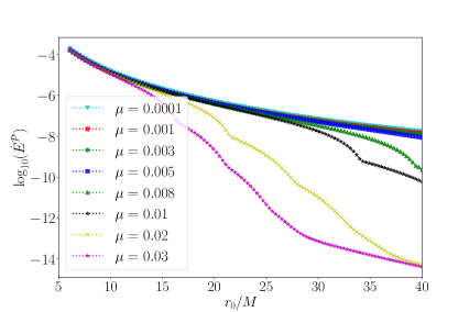
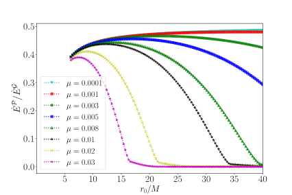
Figure 1: The Proca flux and the ratio between the GW fluxes in the GR and in the Einstein-Proca gravity as a function of the orbital radius $r_{0}/M$ and the Proca mass $\mu$ are plotted, which consider the cases of different Proca field with the masses $\mu\in\{0.0001,0.001,0.003,0.005,0.008,0.01,0.02,0.03\}$.

Fig. 1 displays the Proca and gravitational fluxes ratio $\dot{E}^{\mathcal{P}}/\dot{E}^{\mathcal{G}}$ and the logarithm $\log_{10}(\dot{E}^{\mathcal{P}})$ of the Proca flux as a function of orbital radius $r_{0}/M$, considering the cases of different Proca masses, and the multipole contribution of the fluxes includes the order $l_{\rm max}=10$. One can find that the Proca flux is increasing as the binary objects shrink slowly up to near the ISCO, and the quantitative magnitudes of the Proca fluxes are almost same with the massless case when the Proca mass is $\mu<0.003$. From the bottom of the Fig. 1, the Proca flux near the ISCO can reach to $\sim 40\%$ of the gravitational flux, however, the Proca fluxes are decreasing when the Proca mass is increasing, which would sharp decline for the more massive Proca field. In other word, the Proca flux is suppressed by the Proca mass. Therefore, one can forecast that the deviation of the EMRI dynamics evolution between the Einstein-Proca case and the standard GR case would be more obvious when the vector field becomes heavier.

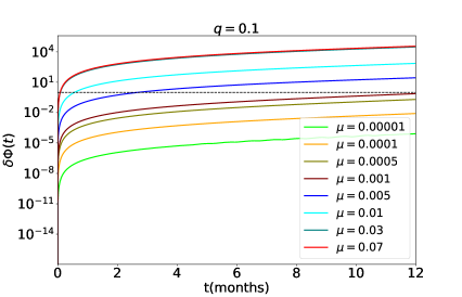
Figure 2: The difference of EMRI orbital phases, for the massive and massless vector fields with the vector charge $q=0.1$, as a function of the observation time are plotted, which contains some cases of the Proca fields with the masses $\mu\in\{0.00001,0.0001,0.0005,0.001,0.005,0.01,0.03,0.07\}$.

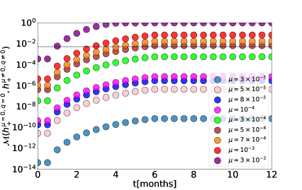
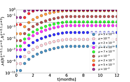
Figure 3: The mismatches between the massless vector field or standard GR cases and the Proca field cases are plotted, where the parameters of the vector fields carried by the smaller objects are $\left(\{\mu=0,q=0\},\{\mu\neq 0,q\neq 0\}\right)$ and $\left(\{\mu=0,q=0.1\},\{\mu\neq 0,q=0.1\}\right)$.

IV.2 dephasing and mismatch

Throughout this paper, the directional parameters related to the EMRI source are fixed as $\theta_{s}=\pi/3,~{}\phi_{s}=\pi/2$, $\theta_{l}=\pi/4,~{}\phi_{l}=\pi/4$, and the initial orbital separation $r_{0}$ is adjusted to experience one-year adiabatic evolution before the final plunge $r_{\text{end}}=r_{\text{ISCO}}+0.1~{}M$. We consider the EMRI system with $m_{p}=10~{}M_{\odot}$, $M=10^{6}~{}M_{\odot}$, the different Proca masses $\mu$, and the luminosity distance $d_{L}$ can be changed freely to vary the SNR of the signal.

To evaluate effect of the Proca field on the EMRI dynamics, we analyse the differences of the orbital phases between the massive and massless vector cases. We compute the dephasing (104) as a function of the observation time in the Fig. 2, where the dashed horizontal line denotes the threshold value $\delta\Phi_{\rm min}=1$ radian discerned by LISA. Note that the difference of two waveform phases is generated by the EMRI systems including the secondary objects with two vector fields $(q=0.1,\mu=0)$ and $(q=0.1,\mu\neq 0)$, where the length of waveforms are both set as one year. According to the Fig. 2, the minimum value of the Proca mass for the charge $q=0.1$ case distinguished by LISA is $\mu_{\rm min}\sim 0.0005$, the dephasing becomes bigger when the Proca field is heavier. The analysis reveals that the lighter Proca field with the mass $\mu\gtrsim 0.0005$ could result in the observable modification effect in the EMRI phase evolution, but the rigorous constraint on the Proca field effect needs to consider the correlation of waveform parameters, such as the mismatch and fisher matrix analysis in the following section.

In order to assess quantifiably the effect of the Proca mass on the EMRI waveforms, the mismatch as a function of the observation time is plotted in Fig. 3, which takes into account the differences of two waveforms between the standard GR case or the massless field case and the Proca field case. It should be noted that the dashed horizontal lines correspond to the threshold value distinguished by LISA in the Fig. 3. Overall, the mismatches grow visibly when the Proca mass is bigger for the fixed vector charge $q=0.1$. The upper panel of the Fig. 3 shows the mismatches for the EMRI systems including the secondaries with the vector field parameters $q=0,\mu=0$ and $q=0.1,\mu\neq 0$, one can see that the minimum value of the Proca mass recognized by LISA is $\mu_{\rm min}\sim 5\times 10^{-4}$ for the vector charge $q=0.1$ case. From the bottom panel of the Fig. 3, the mismatches between the massless vector field case and the Proca field case are plotted, which consider the smaller objects with $q=0.1,\mu=0$ and $q=0.1,\mu\neq 0$. As shown as the bottom panel of the figure, LISA can distinguish the effect of the Proca field with the mass as small as $\mu_{\rm min}\sim 7\times 10^{-4}$.

Our results indicate that, for the Proca field with the mass $\mu\sim 7\times 10^{-4}$ and the charge $q=0.1$, LISA can distinguish the EMRI waveforms including the modification of the massive vector field from the waveforms within the massless vector filed case and the standard GR case. These analysis can be the criterion ruling out some parameters with the EMRI observation, the severe constraint on the Proca field need to consider the parameter estimation using the FIM method in the following subsection.

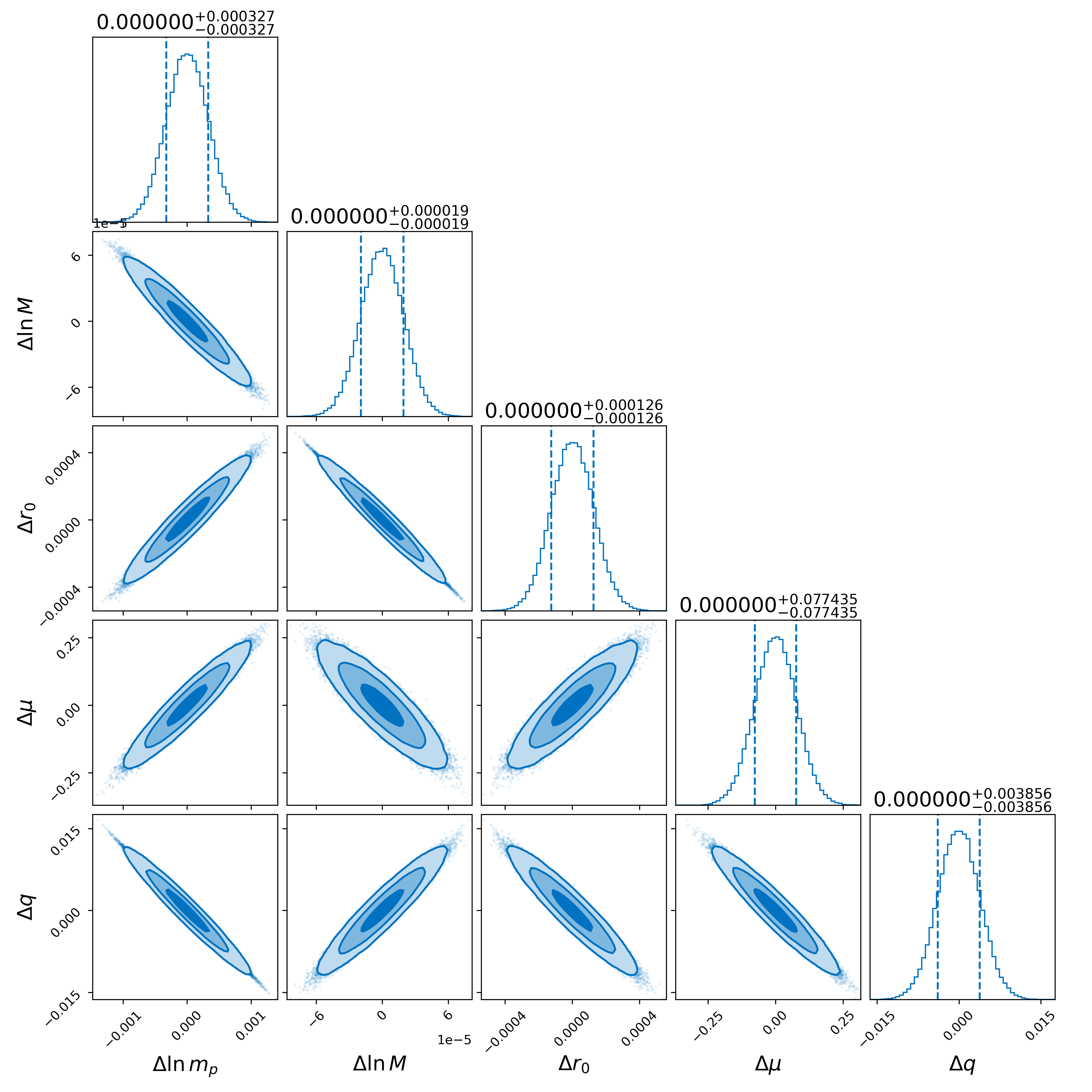
Figure 4: The corner plot for the probability distribution for the Proca field mass, the orbital radius, vector charge, secondary body mass and primary body mass, $(\mu=0.01,r_{0},q,m,M)$, which is inferred from one-year observation of EMRI. Vertical lines show the $1\sigma$ interval for each source parameter. The contours correspond to $68\%$, $95\%$ and $99\%$ probability confidence intervals

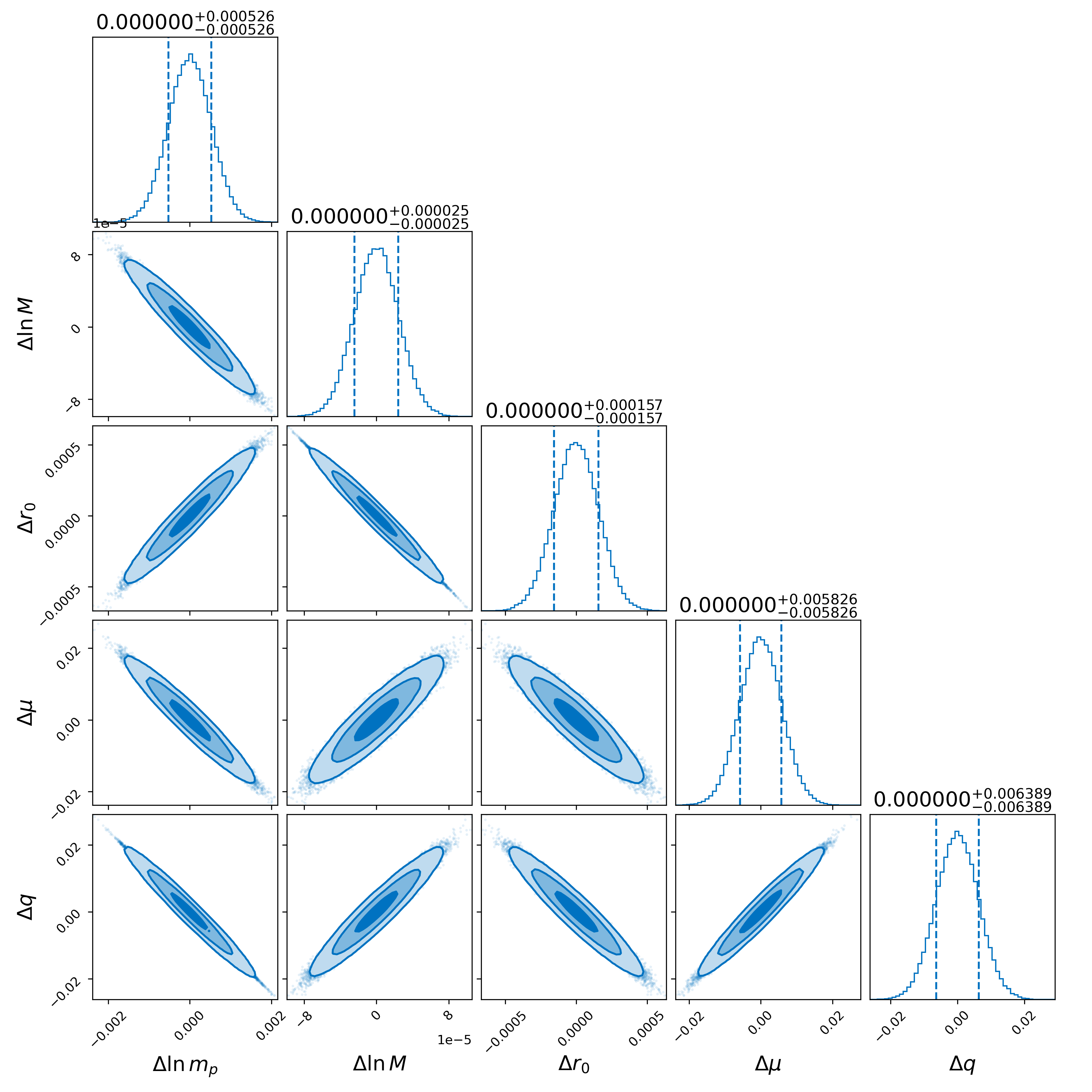
Figure 5: The corner plot for the probability distribution for the Proca field mass, the orbital radius, vector charge, secondary body mass, and primary body mass, $(\mu=0.02,r_{0},q,m,M)$, which is inferred from one-year observation of EMRI. Vertical lines show the $1\sigma$ interval for each source parameter. The contours correspond to $68\%$, $95\%$ and $99\%$ probability confidence intervals

IV.3 Constraint on the Proca field

In this subsection, we plan to adopt the FIM method to compute the constraint on the mass of the Proca field using the EMRI waveform modified by the massive vector field. The measuring errors of EMRI parameters are listed in the Table 2 for the cases of the Proca field masses $\mu=0.01$ and $\mu=0.02$, in which the vector charges of secondaries are set as $q=0.05$. As shown in the table, the constraint accuracy of the Proca field mass can reach a fraction of $\Delta\mu\sim 10^{-2}(\Delta\mu_{v}\sim 1.33\times 10^{-18}\rm eV)$ for the case of $\mu=0.02$, which would slightly be improved comparing with the case of $\mu=0.01$. In Fig. 4 we display the probability distribution of the Proca field mass, the orbital radius, vector charge, secondary body mass, and primary body mass, where the mass and charge of the Proca field are set as $\mu=0.01$ and $q=0.05$. The result for the vector parameters $\mu=0.02$ and $q=0.05$ can be seen in Fig. 5. As shown in Fig. 4 and Fig. 5, the correlation between the Proca mass with other parameters for the case $\mu=0.01$ is inverse to the case $\mu=0.02$. The reason is that the energy flux for the Proca field increases with the Proca mass $\mu$ increases below $\mu\simeq 0.01$, but the Proca flux decreases as the Proca mass increases around $\mu\simeq 0.02$. It’s obvious that for the small Proca mass, including the vector field mass in the EMRI system will add the extra degrees of the vector field case (three propagating degrees), which would increase the Proca flux compared to the massless vector field case (two propagating degrees). However, when the Proca mass increases too much and beyond a certain threshold, the Proca flux will be suppressed by the Proca mass.

$\mu$	$\Delta\mu$	$\Delta q$	$\Delta m_{p}/m_{p}$	$\Delta M/M$	$\Delta r_{0}$
$0.01$	$7.74\times 10^{-2}$	$3.86\times 10^{-3}$	$3.27\times 10^{-4}$	$1.90\times 10^{-5}$	$1.26\times 10^{-4}$
$0.02$	$5.83\times 10^{-3}$	$6.39\times 10^{-3}$	$5.26\times 10^{-4}$	$2.50\times 10^{-5}$	$1.57\times 10^{-4}$

Table 2: Measurement errors of the source parameters using the EMRI waveform modified by the Proca field are listed, the parameters are set as $m_{p}=10~{}M_{\odot}$, $M=10^{6}~{}M_{\odot}$, $q=0.05$ and the SNR of the signal is set as $150$.

V Conclusion

In this paper, we consider the vector charge and mass carried by the secondary object in the EMRI, where the waveform from the inspiral evolution including the extra dipole radiation can be regarded as the probe of detecting the ultralight vector field. We first solve the homogeneous Proca equation and the Regge-Wheeler equation with the ingoing and outgoing boundary conditions, and derive the source term of a point particle on the circular orbits for the Proca field, then derive the energy flux formulas of the Proca field at infinity and near the horizon. Using the independent homogeneous solutions and the source term, one can compute the energy fluxes for the Proca emission and the gravitational emission. We find that the Proca flux would increase as the mass of the vector field increases when the Proca mass is small, but decrease as the mass of the vector field increases when the Proca mass is large.

Under the framework of adiabatic approximation, we evolve the circular orbital parameters of point particle on the equatorial plane, then compute the EMRI waveform using the quadrupole approximation formula. Using the adiabatic EMRI waveforms, we can analyse the effect of the massive vector field on the EMRI waveforms by computing the dephasing and mismatch. Our results show that LISA can distinguish the EMRI waveforms for the Proca field with mass $\mu\sim 7\times 10^{-4}$ from the massless vector field cases. Finally, we carry out the parameter estimation of EMRI source including the modification by the Proca field. According to the constraint computed by the FIM method, the measurement error of the Proca field mass can be controlled within the fraction of $\sim 10^{-2}~{}(\Delta\mu_{v}\sim 1.33\times 10^{-18}\rm eV)$ using the EMRI observation. The constraint on the Proca mass is anti-correlated with the masses $M,m$ of MBH and secondary body, and the correlation would be interesting to include the spin of MBH and the eccentric orbit in the future.

Appendix A Energy fluxes formulas for the massive vector field

From the lagrangian (2), one can compute an effective canonical stress-energy tensor $T^{C}_{\mu\nu}$ for the vector perturbations using the Noether theorem, which can be reduced to the following expression

$$4\pi T^{C}_{\mu\nu}=\frac{\partial\mathcal{L}}{\partial A^{\alpha,\mu}}A^{\alpha}_{~{}~{},\nu}-g_{\mu\nu}\mathcal{L},$$ (117)

where $A^{\alpha,\mu}\equiv\frac{\partial A}{\partial\mu}$ and $A^{\alpha}_{\mu}\equiv\frac{\partial A^{\alpha}}{\partial\nu}$. Using the field equations to further simplify our calculations, we find

$$4\pi T^{C}_{\mu\nu}=F_{\mu\lambda}\partial_{\nu}A^{\lambda}-g_{\mu\nu}\mathcal{L},$$ (118)

there is a general procedure for constructing a symmetric stress tensor

$$4\pi T_{\mu\nu} = F_{\mu\lambda}\partial_{\nu}A^{\lambda}-F_{\mu\lambda}\partial_{\lambda}A^{\nu}-A^{\nu}\partial_{\lambda}F_{\mu\lambda}-g_{\mu\nu}\mathcal{L}$$ (119)

$$+ \frac{\partial}{\partial x^{\lambda}}(F_{\mu\lambda}A^{\nu})$$

$$= g^{\alpha\beta}F_{\mu\alpha}F_{\nu\beta}+\mu_{v}^{2}A_{\mu}A_{\nu}-g_{\mu\nu}\mathcal{L}.$$

The vector fluxes are then given by integrating the components $T_{ti}$, which provide the energy that flows across the unit surface orthogonal to the axis $x^{i}$ per unit time Martel (2004); Zhu and Osburn (2018),

$$\left\langle\frac{dE}{dt}\right\rangle_{H,\infty} = \lim_{r\to r_{h},\infty}\int T_{ti}n^{i}r^{2}d\Omega=$$ (120)

$$- \lim_{r\to r_{h},\infty}\epsilon\int T_{tr}r^{2}fd\Omega,$$

where $\epsilon$ is $1$ corresponding to the flux at the infinity and $\epsilon$ is $-1$ corresponding to the flux near the horizon.

A.1 energy flux at infinity

The vector potential at infinity can be expressed by

$$A_{t} =\frac{\mathcal{A}^{1+}}{r}e^{-i\omega_{m}t}e^{i\sqrt{\omega_{m}^{2}-\mu^{2}}r_{\ast}}r^{\frac{i\mu^{2}}{\sqrt{\omega_{m}^{2}-\mu^{2}}}}Y^{lm},$$

$$A_{r} =\frac{\mathcal{A}^{2+}}{rf}e^{-i\omega_{m}t}e^{i\sqrt{\omega_{m}^{2}-\mu^{2}}r_{\ast}}r^{\frac{i\mu^{2}}{\sqrt{\omega_{m}^{2}-\mu^{2}}}}Y^{lm},$$

$$A_{\theta} =\frac{1}{l(l+1)}\left[\mathcal{A}^{3+}Y^{lm}_{,\theta}+\frac{1}{\sin\theta}\mathcal{A}^{4+}Y^{lm}_{,\phi}\right]$$

$$e^{-i\omega_{m}t}e^{i\sqrt{\omega_{m}^{2}-\mu^{2}}r_{\ast}}r^{\frac{i\mu^{2}}{\sqrt{\omega_{m}^{2}-\mu^{2}}}},$$

$$A_{\phi} =\frac{1}{l(l+1)}\left[\mathcal{A}^{3+}Y^{lm}_{,\phi}-\sin\theta\mathcal{A}^{4+}Y^{lm}_{,\theta}\right]$$ (121)

$$e^{-i\omega_{m}t}e^{i\sqrt{\omega_{m}^{2}-\mu^{2}}r_{\ast}}r^{\frac{i\mu^{2}}{\sqrt{\omega_{m}^{2}-\mu^{2}}}}.$$

Based on the Lorenz condition, we can obtain the following relationship between the $\mathcal{A}^{1+}$ and $\mathcal{A}^{2+}$

$$\omega_{m}\mathcal{A}^{1+}+\sqrt{\omega_{m}^{2}-\mu_{v}^{2}}\mathcal{A}^{2+}=0.$$ (122)

After plugging the expressions Eqs. (A.1) and (122) into the energy flux formula Eq. (120), we can get the energy flux at infinity

$$\lim_{r\to\infty}\left\langle\frac{dE}{dt}\right\rangle = \sum_{l=1}^{\infty}\sum_{m=1}^{l}\frac{\omega_{m}\sqrt{\omega_{m}^{2}-\mu_{v}^{2}}(|\mathcal{A}^{4+}_{lm}|^{2}+|\mathcal{A}_{lm}^{3+}|^{2})}{2\pi l(l+1)}$$ (123)

$$+ \frac{\mu_{v}^{2}}{2\pi}\frac{\sqrt{\omega_{m}^{2}-\mu_{v}^{2}}}{\omega_{m}}|\mathcal{A}^{2+}_{lm}|^{2}.$$

A.2 energy flux near the horizon

At the horizon, the vector potential can be written as following

$$A_{t} = \frac{\mathcal{A}^{1-}}{r}e^{-i\omega_{m}t}e^{-i\omega_{m}r_{\ast}}Y^{lm},$$

$$A_{r} = \frac{\mathcal{A}^{2-}}{rf}e^{-i\omega_{m}t}e^{-i\omega_{m}r_{\ast}}Y^{lm},$$

$$A_{\theta} = \frac{1}{l(l+1)}\left[\mathcal{A}^{3-}Y^{lm}_{,\theta}+\frac{1}{\sin\theta}\mathcal{A}^{4-}Y^{lm}_{,\phi}\right]e^{-i\omega_{m}t}e^{-i\omega_{m}r_{\ast}},$$

$$A_{\phi} = \frac{1}{l(l+1)}\left[\mathcal{A}^{3-}Y^{lm}_{,\phi}-\sin\theta\mathcal{A}^{4-}Y^{lm}_{,\theta}\right]e^{-i\omega_{m}t}e^{-i\omega_{m}r_{\ast}},$$

where $Y^{lm}_{,\theta}\equiv\frac{\partial Y^{lm}}{\partial\theta}$ and $Y^{lm}_{,\phi}\equiv\frac{\partial Y^{lm}}{\partial\phi}$ . Based on the Lorenz condition, we can get the following relationship between the $\mathcal{A}^{1-}$ and $\mathcal{A}^{2-}$

$$\mathcal{A}^{1-}-\mathcal{A}^{2-}=0.$$ (125)

After plugging the expressions Eqs. (A.2) and (125) into the energy flux formula Eq. (120), we can get at the horizon

$$\begin{split}\lim_{r\to r_{h}}\left\langle\frac{dE}{dt}\right\rangle=&\sum_{l=1}^{\infty}\sum_{m=1}^{l}\frac{\omega_{m}^{2}|\mathcal{A}^{4-}_{lm}|^{2}}{2\pi l(l+1)}+\frac{\omega_{m}^{2}|\mathcal{A}^{3-}_{lm}|^{2}}{2\pi l(l+1)}\\ &+\frac{l(l+1)+4\mu_{v}^{2}}{8\pi}|\mathcal{A}^{2-}_{lm}|^{2}\\ &-\frac{i\omega_{m}}{4\pi}\left(\mathcal{A}^{2-}_{lm}\mathcal{A}^{3-\ast}_{lm}-\mathcal{A}^{3-}_{lm}\mathcal{A}^{2-\ast}_{lm}\right).\end{split}$$ (126)

References

- Goodsell et al. (2009) M. Goodsell, J. Jaeckel, J. Redondo, and A. Ringwald, Naturally Light Hidden Photons in LARGE Volume String Compactifications, J. High Energ. Phys. 11 (2009) 027.
- Essig et al. (2013) R. Essig et al., in Snowmass 2013: Snowmass on the Mississippi (2013) arXiv:1311.0029 .
- Brito et al. (2015) R. Brito, V. Cardoso, and P. Pani, Superradiance: New Frontiers in Black Hole Physics, Lect. Notes Phys. 906, pp.1 (2015).
- Dolan (2007) S. R. Dolan, Instability of the massive Klein-Gordon field on the Kerr spacetime, Phys. Rev. D 76, 084001 (2007).
- Arvanitaki et al. (2017) A. Arvanitaki, M. Baryakhtar, S. Dimopoulos, S. Dubovsky, and R. Lasenby, Black Hole Mergers and the QCD Axion at Advanced LIGO, Phys. Rev. D 95, 043001 (2017).
- Arvanitaki et al. (2015) A. Arvanitaki, M. Baryakhtar, and X. Huang, Discovering the QCD Axion with Black Holes and Gravitational Waves, Phys. Rev. D 91, 084011 (2015).
- Pani et al. (2012a) P. Pani, V. Cardoso, L. Gualtieri, E. Berti, and A. Ishibashi, Black hole bombs and photon mass bounds, Phys. Rev. Lett. 109, 131102 (2012a).
- Pani et al. (2012b) P. Pani, V. Cardoso, L. Gualtieri, E. Berti, and A. Ishibashi, Perturbations of slowly rotating black holes: massive vector fields in the Kerr metric, Phys. Rev. D 86, 104017 (2012b).
- Witek et al. (2013) H. Witek, V. Cardoso, A. Ishibashi, and U. Sperhake, Superradiant instabilities in astrophysical systems, Phys. Rev. D 87, 043513 (2013).
- East and Pretorius (2017) W. E. East and F. Pretorius, Superradiant Instability and Backreaction of Massive Vector Fields around Kerr Black Holes, Phys. Rev. Lett. 119, 041101 (2017).
- East (2018) W. E. East, Massive Boson Superradiant Instability of Black Holes: Nonlinear Growth, Saturation, and Gravitational Radiation, Phys. Rev. Lett. 121, 131104 (2018).
- Dolan (2018) S. R. Dolan, Instability of the Proca field on Kerr spacetime, Phys. Rev. D 98, 104006 (2018).
- Siemonsen and East (2020) N. Siemonsen and W. E. East, Gravitational wave signatures of ultralight vector bosons from black hole superradiance, Phys. Rev. D 101, 024019 (2020).
- Brito et al. (2017) R. Brito, S. Ghosh, E. Barausse, E. Berti, V. Cardoso, I. Dvorkin, A. Klein, and P. Pani, Gravitational wave searches for ultralight bosons with LIGO and LISA, Phys. Rev. D 96, 064050 (2017).
- Jones et al. (2023) D. Jones, L. Sun, N. Siemonsen, W. E. East, S. M. Scott, and K. Wette, Methods and prospects for gravitational-wave searches targeting ultralight vector-boson clouds around known black holes, Phys. Rev. D 108, 064001 (2023).
- Abac et al. (2024) A. G. Abac et al. (LIGO Scientific, VIRGO, KAGRA), Ultralight vector dark matter search using data from the KAGRA O3GK run, arXiv:2403.03004 .
- Michimura et al. (2020) Y. Michimura, T. Fujita, S. Morisaki, H. Nakatsuka, and I. Obata, Ultralight vector dark matter search with auxiliary length channels of gravitational wave detectors, Phys. Rev. D 102, 102001 (2020).
- Miller and Mendes (2023) A. L. Miller and L. Mendes, First search for ultralight dark matter with a space-based gravitational-wave antenna: LISA Pathfinder, Phys. Rev. D 107, 063015 (2023).
- Vermeulen et al. (2021) S. M. Vermeulen et al., Direct limits for scalar field dark matter from a gravitational-wave detector, arXiv:2103.03783 .
- Hui et al. (2017) L. Hui, J. P. Ostriker, S. Tremaine, and E. Witten, Ultralight scalars as cosmological dark matter, Phys. Rev. D 95, 043541 (2017).
- Miller et al. (2021) A. L. Miller, S. Clesse, F. De Lillo, G. Bruno, A. Depasse, and A. Tanasijczuk, Probing planetary-mass primordial black holes with continuous gravitational waves, Phys. Dark Univ. 32, 100836 (2021).
- Chen et al. (2017) S.-R. Chen, H.-Y. Schive, and T. Chiueh, Jeans Analysis for Dwarf Spheroidal Galaxies in Wave Dark Matter, Mon. Not. R. Astron. Soc. 468, 1338 (2017).
- Nelson and Scholtz (2011) A. E. Nelson and J. Scholtz, Dark Light, Dark Matter and the Misalignment Mechanism, Phys. Rev. D 84, 103501 (2011).
- Graham et al. (2016) P. W. Graham, J. Mardon, and S. Rajendran, Vector Dark Matter from Inflationary Fluctuations, Phys. Rev. D 93, 103520 (2016).
- Schlamminger et al. (2008) S. Schlamminger, K. Y. Choi, T. A. Wagner, J. H. Gundlach, and E. G. Adelberger, Test of the equivalence principle using a rotating torsion balance, Phys. Rev. Lett. 100, 041101 (2008).
- Williams et al. (2004) J. G. Williams, S. G. Turyshev, and D. H. Boggs, Progress in lunar laser ranging tests of relativistic gravity, Phys. Rev. Lett. 93, 261101 (2004).
- Turyshev and Williams (2007) S. G. Turyshev and J. G. Williams, Space-based tests of gravity with laser ranging, Int. J. Mod. Phys. D 16, 2165 (2007).
- Siemonsen et al. (2023) N. Siemonsen, T. May, and W. E. East, Modeling the black hole superradiance gravitational waveform, Phys. Rev. D 107, 104003 (2023).
- Fell et al. (2023) S. D. B. Fell, L. Heisenberg, and D. Veske, Detecting fundamental vector fields with LISA, Phys. Rev. D 108, 083010 (2023).
- Berry et al. (2019) C. P. L. Berry, S. A. Hughes, C. F. Sopuerta, A. J. K. Chua, A. Heffernan, K. Holley-Bockelmann, D. P. Mihaylov, M. C. Miller, and A. Sesana, The unique potential of extreme mass-ratio inspirals for gravitational-wave astronomy, arXiv:1903.03686 .
- Berti et al. (2019) E. Berti et al., Tests of General Relativity and Fundamental Physics with Space-based Gravitational Wave Detectors, arXiv:1903.02781 .
- Babak et al. (2017) S. Babak, J. Gair, A. Sesana, E. Barausse, C. F. Sopuerta, C. P. L. Berry, E. Berti, P. Amaro-Seoane, A. Petiteau, and A. Klein, Science with the space-based interferometer LISA. V: Extreme mass-ratio inspirals, Phys. Rev. D 95, 103012 (2017).
- Zi et al. (2021) T.-G. Zi, J.-D. Zhang, H.-M. Fan, X.-T. Zhang, Y.-M. Hu, C. Shi, and J. Mei, Science with the TianQin Observatory: Preliminary results on testing the no-hair theorem with extreme mass ratio inspirals, Phys. Rev. D 104, 064008 (2021).
- Cárdenas-Avendaño and Sopuerta (2024) A. Cárdenas-Avendaño and C. F. Sopuerta, Testing gravity with Extreme-Mass-Ratio Inspirals, arXiv:2401.08085 .
- Cardoso et al. (2022) V. Cardoso, K. Destounis, F. Duque, R. Panosso Macedo, and A. Maselli, Gravitational Waves from Extreme-Mass-Ratio Systems in Astrophysical Environments, Phys. Rev. Lett. 129, 241103 (2022).
- Duque et al. (2023) F. Duque, C. F. B. Macedo, R. Vicente, and V. Cardoso, Axion Weak Leaks: extreme mass-ratio inspirals in ultra-light dark matter, arXiv:2312.06767 .
- Speeney et al. (2024) N. Speeney, E. Berti, V. Cardoso, and A. Maselli, Black holes surrounded by generic matter distributions: Polar perturbations and energy flux, Phys. Rev. D 109, 084068 (2024).
- Rahman et al. (2024) M. Rahman, S. Kumar, and A. Bhattacharyya, Probing astrophysical environment with eccentric extreme mass-ratio inspirals, J. Cosmol. Astropart. Phys. 01 (2024) 035.
- Cole et al. (2023) P. S. Cole, G. Bertone, A. Coogan, D. Gaggero, T. Karydas, B. J. Kavanagh, T. F. M. Spieksma, and G. M. Tomaselli, Distinguishing environmental effects on binary black hole gravitational waveforms, Nat. Astron. 7, 943 (2023).
- Zhang et al. (2024) C. Zhang, G. Fu, and N. Dai, Detecting dark matter halos with extreme mass-ratio inspirals, J. Cosmol. Astropart. Phys. 04 (2024) 088.
- Brito and Shah (2023) R. Brito and S. Shah, Extreme mass-ratio inspirals into black holes surrounded by scalar clouds, Phys. Rev. D 108, 084019 (2023).
- Glampedakis (2005) K. Glampedakis, Extreme mass ratio inspirals: LISA’s unique probe of black hole gravity, Classical Quantum Gravity 22, S605 (2005).
- Fan et al. (2020) H.-M. Fan, Y.-M. Hu, E. Barausse, A. Sesana, J.-d. Zhang, X. Zhang, T.-G. Zi, and J. Mei, Science with the TianQin observatory: Preliminary result on extreme-mass-ratio inspirals, Phys. Rev. D 102, 063016 (2020).
- Berti et al. (2015) E. Berti et al., Testing General Relativity with Present and Future Astrophysical Observations, Classical Quantum Gravity 32, 243001 (2015).
- Barack et al. (2019) L. Barack et al., Black holes, gravitational waves and fundamental physics: a roadmap, Classical Quantum Gravity 36, 143001 (2019).
- Bonga et al. (2019) B. Bonga, H. Yang, and S. A. Hughes, Tidal resonance in extreme mass-ratio inspirals, Phys. Rev. Lett. 123, 101103 (2019).
- Pan and Yang (2021) Z. Pan and H. Yang, Formation Rate of Extreme Mass Ratio Inspirals in Active Galactic Nuclei, Phys. Rev. D 103, 103018 (2021).
- Pan et al. (2023) Z. Pan, H. Yang, L. Bernard, and B. Bonga, Resonant dynamics of extreme mass-ratio inspirals in a perturbed Kerr spacetime, Phys. Rev. D 108, 104026 (2023).
- Dai et al. (2023) N. Dai, Y. Gong, Y. Zhao, and T. Jiang, Extreme mass ratio inspirals in galaxies with dark matter halos, arXiv:2301.05088 .
- Figueiredo et al. (2023) E. Figueiredo, A. Maselli, and V. Cardoso, Black holes surrounded by generic dark matter profiles: Appearance and gravitational-wave emission, Phys. Rev. D 107, 104033 (2023).
- Zi and Li (2023) T. Zi and P.-C. Li, Gravitational waves from extreme-mass-ratio inspirals around a hairy Kerr black hole, Phys. Rev. D 108, 084001 (2023).
- Maselli et al. (2020) A. Maselli, N. Franchini, L. Gualtieri, and T. P. Sotiriou, Detecting scalar fields with Extreme Mass Ratio Inspirals, Phys. Rev. Lett. 125, 141101 (2020).
- Maselli et al. (2022) A. Maselli, N. Franchini, L. Gualtieri, T. P. Sotiriou, S. Barsanti, and P. Pani, Detecting fundamental fields with LISA observations of gravitational waves from extreme mass-ratio inspirals, Nat. Astron. 6, 464 (2022).
- Barsanti et al. (2022) S. Barsanti, N. Franchini, L. Gualtieri, A. Maselli, and T. P. Sotiriou, Extreme mass-ratio inspirals as probes of scalar fields: Eccentric equatorial orbits around Kerr black holes, Phys. Rev. D 106, 044029 (2022).
- Barsanti et al. (2023) S. Barsanti, A. Maselli, T. P. Sotiriou, and L. Gualtieri, Detecting Massive Scalar Fields with Extreme Mass-Ratio Inspirals, Phys. Rev. Lett. 131, 051401 (2023).
- Zhang et al. (2023a) C. Zhang, Y. Gong, D. Liang, and B. Wang, Gravitational waves from eccentric extreme mass-ratio inspirals as probes of scalar fields, J. Cosmol. Astropart. Phys. 06 (2023) 054.
- Zhang et al. (2023b) C. Zhang, H. Guo, Y. Gong, and B. Wang, Detecting vector charge with extreme mass ratio inspirals onto Kerr black holes, J. Cosmol. Astropart. Phys. 06 (2023) 020.
- Della Rocca et al. (2024) M. Della Rocca, S. Barsanti, L. Gualtieri, and A. Maselli, Extreme mass-ratio inspirals as probes of scalar fields: inclined circular orbits around Kerr black holes, arXiv:2401.09542 .
- Mignemi and Stewart (1993) S. Mignemi and N. R. Stewart, Charged black holes in effective string theory, Phys. Rev. D 47, 5259 (1993).
- Kleihaus et al. (2011) B. Kleihaus, J. Kunz, and E. Radu, Rotating Black Holes in Dilatonic Einstein-Gauss-Bonnet Theory, Phys. Rev. Lett. 106, 151104 (2011).
- Antoniou et al. (2018a) G. Antoniou, A. Bakopoulos, and P. Kanti, Evasion of No-Hair Theorems and Novel Black-Hole Solutions in Gauss-Bonnet Theories, Phys. Rev. Lett. 120, 131102 (2018a).
- Antoniou et al. (2018b) G. Antoniou, A. Bakopoulos, and P. Kanti, Black-Hole Solutions with Scalar Hair in Einstein-Scalar-Gauss-Bonnet Theories, Phys. Rev. D 97, 084037 (2018b).
- Doneva and Yazadjiev (2018) D. D. Doneva and S. S. Yazadjiev, New Gauss-Bonnet Black Holes with Curvature-Induced Scalarization in Extended Scalar-Tensor Theories, Phys. Rev. Lett. 120, 131103 (2018).
- Chagoya et al. (2016) J. Chagoya, G. Niz, and G. Tasinato, Black Holes and Abelian Symmetry Breaking, Classical Quantum Gravity 33, 175007 (2016).
- Minamitsuji (2016) M. Minamitsuji, Solutions in the generalized Proca theory with the nonminimal coupling to the Einstein tensor, Phys. Rev. D 94, 084039 (2016).
- Babichev et al. (2017) E. Babichev, C. Charmousis, and M. Hassaine, Black holes and solitons in an extended Proca theory, J. High Energ. Phys. 05 (2017) 114.
- Herdeiro et al. (2016) C. Herdeiro, E. Radu, and H. Rúnarsson, Kerr black holes with Proca hair, Classical Quantum Gravity 33, 154001 (2016).
- Heisenberg et al. (2017) L. Heisenberg, R. Kase, M. Minamitsuji, and S. Tsujikawa, Hairy black-hole solutions in generalized Proca theories, Phys. Rev. D 96, 084049 (2017).
- Kase et al. (2018a) R. Kase, M. Minamitsuji, and S. Tsujikawa, Black holes in quartic-order beyond-generalized Proca theories, Phys. Lett. B 782, 541 (2018a).
- Kase et al. (2018b) R. Kase, M. Minamitsuji, S. Tsujikawa, and Y.-L. Zhang, Black hole perturbations in vector-tensor theories: The odd-mode analysis, J. Cosmol. Astropart. Phys. 02 (2018) 048.
- Minamitsuji (2017) M. Minamitsuji, Proca stars with nonminimal coupling to the Einstein tensor, Phys. Rev. D 96, 044017 (2017).
- Kase et al. (2018c) R. Kase, M. Minamitsuji, and S. Tsujikawa, Relativistic stars in vector-tensor theories, Phys. Rev. D 97, 084009 (2018c).
- Kase et al. (2020) R. Kase, M. Minamitsuji, and S. Tsujikawa, Neutron stars with a generalized Proca hair and spontaneous vectorization, Phys. Rev. D 102, 024067 (2020).
- Ramazanoğlu and Pretorius (2016) F. M. Ramazanoğlu and F. Pretorius, Spontaneous Scalarization with Massive Fields, Phys. Rev. D 93, 064005 (2016).
- Nair et al. (2019) R. Nair, S. Perkins, H. O. Silva, and N. Yunes, Fundamental Physics Implications for Higher-Curvature Theories from Binary Black Hole Signals in the LIGO-Virgo Catalog GWTC-1, Phys. Rev. Lett. 123, 191101 (2019).
- Garcia-Saenz et al. (2021) S. Garcia-Saenz, A. Held, and J. Zhang, Destabilization of Black Holes and Stars by Generalized Proca Fields, Phys. Rev. Lett. 127, 131104 (2021).
- Rosa and Dolan (2012) J. G. Rosa and S. R. Dolan, Massive vector fields on the Schwarzschild spacetime: quasi-normal modes and bound states, Phys. Rev. D 85, 044043 (2012).
- Poisson (1993) E. Poisson, Gravitational radiation from a particle in circular orbit around a black hole. 1: Analytical results for the nonrotating case, Phys. Rev. D 47, 1497 (1993).
- Zhu and Osburn (2018) R. Zhu and T. Osburn, Inspirals into a charged black hole, Phys. Rev. D 97, 104058 (2018).
- Martel (2004) K. Martel, Gravitational wave forms from a point particle orbiting a Schwarzschild black hole, Phys. Rev. D 69, 044025 (2004).
- Regge and Wheeler (1957) T. Regge and J. A. Wheeler, Stability of a Schwarzschild singularity, Phys. Rev. 108, 1063 (1957).
- Zerilli (1970) F. J. Zerilli, Effective potential for even parity Regge-Wheeler gravitational perturbation equations, Phys. Rev. Lett. 24, 737 (1970).
- (83) Black Hole Perturbation Toolkit, (bhptoolkit.org).
- Barack and Cutler (2004) L. Barack and C. Cutler, LISA capture sources: Approximate waveforms, signal-to-noise ratios, and parameter estimation accuracy, Phys. Rev. D 69, 082005 (2004).
- Huerta and Gair (2011) E. A. Huerta and J. R. Gair, Importance of including small body spin effects in the modelling of extreme and intermediate mass-ratio inspirals, Phys. Rev. D 84, 064023 (2011).
- Jiang et al. (2022) T. Jiang, N. Dai, Y. Gong, D. Liang, and C. Zhang, Constraint on Brans-Dicke theory from intermediate/extreme mass ratio inspirals, J. Cosmol. Astropart. Phys. 12 (2022) 023.
- Babak et al. (2007) S. Babak, H. Fang, J. R. Gair, K. Glampedakis, and S. A. Hughes, ’Kludge’ gravitational waveforms for a test-body orbiting a Kerr black hole, Phys. Rev. D 75, 024005 (2007), [Erratum: Phys.Rev.D 77, 04990 (2008)].
- Amaro-Seoane et al. (2017) P. Amaro-Seoane et al. (LISA), Laser Interferometer Space Antenna, arXiv:1702.00786 .
- Mei et al. (2021) J. Mei et al. (TianQin), The TianQin project: current progress on science and technology, PTEP 2021, 05A107 (2021).
- Gong et al. (2021) Y. Gong, J. Luo, and B. Wang, Concepts and status of Chinese space gravitational wave detection projects, Nat. Astron. 5, 881 (2021).
- Cutler et al. (1994) C. Cutler, D. Kennefick, and E. Poisson, Gravitational radiation reaction for bound motion around a Schwarzschild black hole, Phys. Rev. D 50, 3816 (1994).
- Flanagan and Hughes (1998) E. E. Flanagan and S. A. Hughes, Measuring gravitational waves from binary black hole coalescences: 2. The Waves’ information and its extraction, with and without templates, Phys. Rev. D 57, 4566 (1998).
- Lindblom et al. (2008) L. Lindblom, B. J. Owen, and D. A. Brown, Model Waveform Accuracy Standards for Gravitational Wave Data Analysis, Phys. Rev. D 78, 124020 (2008).
- Berti et al. (2012) E. Berti, L. Gualtieri, M. Horbatsch, and J. Alsing, Light scalar field constraints from gravitational-wave observations of compact binaries, Phys. Rev. D 85, 122005 (2012).