Zero-Shot Generalization during Instruction Tuning:
Insights from Similarity and Granularity

Abstract

Understanding alignment techniques begins with comprehending zero-shot generalization brought by instruction tuning, but little of the mechanism has been understood. Existing work has largely been confined to the task level, without considering that tasks are artificially defined and, to LLMs, merely consist of tokens and representations. This line of research has been limited to examining transfer between tasks from a task-pair perspective, with few studies focusing on understanding zero-shot generalization from the perspective of the data itself. To bridge this gap, we first demonstrate through multiple metrics that zero-shot generalization during instruction tuning happens very early. Next, we investigate the facilitation of zero-shot generalization from both data similarity and granularity perspectives, confirming that encountering highly similar and fine-grained training data earlier during instruction tuning, without the constraints of defined “tasks”, enables better generalization. Finally, we propose a more grounded training data arrangement method, Test-centric Multi-turn Arrangement, and show its effectiveness in promoting continual learning and further loss reduction. For the first time, we show that zero-shot generalization during instruction tuning is a form of similarity-based generalization between training and test data at the instance level. We hope our analysis will advance the understanding of zero-shot generalization during instruction tuning and contribute to the development of more aligned LLMs.

1 Introduction

The extraordinariness of large language models (LLMs) was originally brought by the zero-shot generalization of instruction tuning [2]. At the early stage, studies have found that when diverse prompts are added to the inputs of traditional natural language processing (NLP) tasks and fed into the model for instruction tuning, the model can generalize to tasks it has never encountered before [5, 24, 37, 47, 48]. To date, instruction tuning [5, 37, 48] has become a crucial phase in training large language models, often preceding methods that incorporate preference data. In the meantime, the concept of “task” is also becoming increasingly blurred. Researchers are no longer constructing instruction data in the ways traditional NLP tasks dictate, but rather, they hope these tasks will be as close to reality and as diverse as possible [4, 11, 35, 41, 54].

Although nearly all LLMs benefit from the zero-shot generalization brought about by instruction tuning, the in-depth and fine-grained research on this phenomenon is still insufficient. Particularly, there are few accurate and comprehensive conclusions about when and in what form it occurs, and how the data could influence it. A line of research focuses on understanding the relationships in task-pair transfer [40, 45, 52], suggesting that not all tasks contribute positively to zero-shot generalization; some tasks may even result in negative transfer effects [21, 26, 56]. The main limitation of the existing works is that they are confined within the concept of “task”. Whether they train on one task and then evaluate on another [21, 56], or simply calculate intermediate task [45] or instruction [22] transfer scores, all these efforts to select the most informative tasks to promote zero-shot generalization are restricted to the task-based framework. This approach is based on the premise that human-defined “tasks” and even “categories” are sufficiently reasonable. However, this is often not the case as gaps exist regarding how humans and LLMs perceive the instruction tuning data. To this end, we strive to break free from the task-level framework and explore “generalization” at a more fundamental level.

In this paper, we conduct a comprehensive investigation of the zero-shot generalization during instruction tuning and attempt to answer some critical questions: In instruction tuning, i) when does zero-shot generalization occur? ii) How can we more accurately understand the role of data in zero-shot generalization? iii) How can we effectively promote zero-shot generalization?

To answer the first research question, we attempt to pinpoint the timing of zero-shot generalization during instruction tuning in. In line with existing works [3, 16, 53, 55], we discover that zero-shot generalization occurs extremely early regardless of the metrics we apply for measurement. This indicates that LLM’s instruction-following ability could be unlocked by leveraging merely a few sample training data. In addition, we find loss as a stable and fair indicator of zero-shot generalization during our measurement. (Section 2)

To further investigate why zero-shot generalization occurs early, we explore the impact brought by different data permutations, demonstrating that training data itself plays an important role during the early stage of instruction tuning. Diving deeper, we identify two perspectives in understanding this role: similarity and granularity. From a similarity perspective, we discover that the model’s generalization is not truly “zero-shot”, as a high resemblance between the test and training data distributions could significantly impact generalization. To quantify the similarity, we define Weighted Similarity Distance (WSD), taking into account both the average and minimum cosine similarity (Cosine-Avg and Cosine-Min) between the training data seen by the model and the test data. Our experiments reveal that encountering data with high similarity (low WSD) early during instruction tuning enhances zero-shot generalization compared to encountering such data later. From a granularity perspective, we disclose that artificially defined “tasks” are no longer suitable for measuring generalization. Instead, the similarity between training data and test data serves as a more essential indicator. By treating all data points equally and considering them at the instance level without the constraints of pre-defined “tasks,” we can better promote zero-shot generalization. (Section 3)

Though the WSD measure shows effectiveness in promoting zero-shot generalization, it still suffers from inherent limitations in that the individual role of each test data point cannot be distinguished, as the whole test set is considered holistically during distance calculation. To this end, we propose the Test-centric Multi-turn Arrangement (TMA). TMA arranges training data according to each individual test data point and seeks to enhance zero-shot generalization regardless of the presence of predefined “tasks.” We demonstrate through experiments the effectiveness of TMA, and unveil that early access to data of higher similarity during instruction tuning can facilitate continual learning and further loss reduction. (Section 4)

We summarize our contributions as follows:

• We show that zero-shot generalization occurs at the very early stage during instruction tuning, while loss serves as a reasonable and suitable metric to measure zero-shot generalization due to its stability and fairness across datasets.

• We identify similarity and granularity as two perspectives to gain a deeper understanding of zero-shot generalization, revealing that encountering highly similar and fine-grained training data earlier during instruction tuning, enables better generalization.

• We propose the Test-centric Multi-turn Arrangement, a more grounded training data arrangement method, and show that accessing high-similarity data during instruction tuning can facilitate continual learning and further loss reduction.

2 Positioning Zero-Shot Generalization

Early research shows that instruction tuning, which applies to various NLP tasks formatted with instructions, can generalize to various unseen tasks. However, most studies [5, 19, 24] focus on integrating diverse tasks or instruction templates, using human-generated or synthetic data, or exploring different fine-tuning strategies, while few studies address when zero-shot generalization actually occurs. Therefore, to bridge this gap, we seek to identify the positioning of zero-shot generalization. We begin by giving a formalization of zero-shot generalization.

Formalization. In multi-task scenarios, zero-shot generalization refers to the ability to perform effectively on unseen tasks, while only trained on a subset of tasks. For each task $T\in\mathcal{D}_{\text{Seen}}\cup\mathcal{D}_{\text{Unseen}}$, there exists an instructional description $I^{T}$, as well as several instances, where each instance is composed of an input $x^{T}_{i}$ and an output $y^{T}_{i}$. We define a model $M$ as capable of generalization on unseen tasks if, after training on every $T\in\mathcal{D}_{\text{Seen}}$, given an unseen task $T\in\mathcal{D}_{\text{Unseen}}$, and for any $(x^{T}_{i},y^{T}_{i})$, the model’s output $\hat{y}=M(I^{T},x^{T}_{i})$ and the label $y^{T}_{i}$ achieve a score surpassing a certain threshold, with regard to the selected metrics, indicating successful generalization on the task $T$.

2.1 Occurrence of Zero-Shot Generalization in Instruction Tuning

From the formalization above, it is clear that the measurement of zero-shot generalization is largely dependent upon the selection of metrics. However, the impact of various metrics on zero-shot generalization is rarely studied. To this end, we first evaluate multiple metrics to see if they are suitable for zero-shot generalization and demonstrate that: [couleur= msftBlack!05, epBord=1, arrondi=0.1, logo=, marge=6, ombre=true, blur, couleurBord=msftBlack!10, tailleOndu=2, sousTitre =Takeaway 1: Zero-shot generalization occurs during the very early stage of instruction tuning, despite the metrics chosen for measurement.]

Data and Settings. We utilize three multi-task datasets, namely Natural Instructions V2 (NIV2) [47], Public Pool of Prompts (P3) [37], and Flan-mini [14], for our analysis. For NIV2, we utilize the default track and default training-test split for instruction tuning and evaluation. For P3, we employ training and test tasks consistent with the vanilla T0 model. For Flan-mini, we randomly partition the training and test tasks. And we choose pre-trained LLaMA-2-7B [43] as our base model. For other details including dataset details, hyper-parameters, data concatenation, and prompt template, please refer to Appendix A. All subsequent experiments are based on this setup, where we adopt a fine-grained approach to save a series of full-parameter fine-tuning checkpoints, evaluating each on the test set to observe the results on the specified metric.

Metrics. Evaluation metrics are crucial for assessing generalization. For datasets including P3, Flan-mini, and OPT-IML [19], Exact-Match is commonly applied due to its simplicity. NIV2 additionally incorporates ROUGE-1 and ROUGE-L as metrics. Besides, in reinforcement learning scenarios, the reward model (RM) plays a vital role [7, 51], serving as a proxy for human preferences. This makes the RM score also a reasonable metric to reflect zero-shot generalization.

To comprehensively study the impact of metrics, we apply all the metrics listed above, including Exact-Match, ROUGE-1, ROUGE-L, and RM score, in our preliminary study. Especially, for the RM score, we use UltraRM-13B [7] as the reward model.

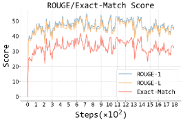
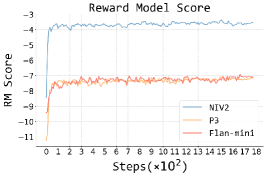
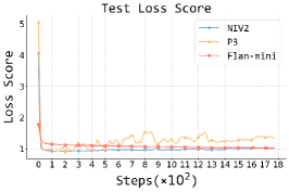
Figure 1: Average ROUGE-1, ROUGE-L, and Exact-Match scores (left), average RM scores (middle), and average loss scores (right) of checkpoints fine-tuned on NIV2 (left, middle, right), P3 (middle, right), and Flan-mini (middle, right), all evaluated on unseen tasks.

Results. We demonstrate that zero-shot generalization occurs at a very early stage during instruction tuning. As depicted in the left plot of Figure 1, using ROUGE-1, ROUGE-L, and Exact-Match as metrics, the ROUGE scores rise from approximately 15 to over 35 in just about 10 training steps, indicating significant generalization with only around 160 training samples. In the middle plot, the RM score exhibits a similar trend, stabilizing around 50 steps across all three datasets.

It is also noteworthy that all these metrics exhibit certain problems: ROUGE-1, ROUGE-L, and Exact-Match as metrics entail the resulting curves being seriously unstable, while the RM score for NIV2 is significantly higher than those for the other two datasets, indicating a certain bias induced. We provide a more detailed discussion in Section A.5. Therefore, we seek to apply a more reasonable metric as an indicator to evaluate zero-shot generalization.

2.2 Loss as the Measurement for Zero-Shot Generalization

Loss is commonly applied across various model pre-training and fine-tuning scenarios. For example, the scaling law [6, 17, 20] entails predicting loss based on model parameter count and dataset size, unsupervised learning uses cross-entropy loss to quantify the difference between probability distribution, etc. Recent studies have also delved into understanding emergent abilities from the perspective of loss, indicating that when pre-training loss drops below a specific threshold, the model can perform well on downstream tasks [12]. All these measures suggest loss to be a promising metric for evaluating generalization on unseen tasks. However, no currently established practice applies it to measure zero-shot generalization. To bridge this gap, we comprehensively study and justify that:

[couleur= msftBlack!05, epBord=1, arrondi=0.1, logo=, marge=6, ombre=true, blur, couleurBord=msftBlack!10, tailleOndu=2, sousTitre =Takeaway 2: Loss serves as a reasonable and suitable metric to measure zero-shot generalization due to its stability and fairness across datasets.]

Data and Settings. We use the same dataset as in the previous experiment. We randomly sample 120 data points from all unseen tasks and generate outputs using a series of instruction-tuned checkpoints. We then calculate the average cross-entropy loss against the corresponding labels within each step. This also entails the same setting as in the previous experiment. Please refer to Section A.4 for more details.

Results. Zero-shot generalization similarly occurs at an early stage of instruction tuning with loss as the evaluation metric. As shown in the right plot of Figure 1, all three datasets reach their lowest points in terms of loss within less than 50 steps, which further strengthens our conclusion that zero-shot generalization occurs early.

Moreover, compared to the left and middle plots in  Figure 1, it is noteworthy that loss as an indicator is more stable and fair across different datasets, entailing it as a more reasonable metric for the measurement. We also provide a case study of loss curves with regard to different unseen tasks, as detailed in Section A.6.

3 Facilitating Zero-Shot Generalization

Acknowledging the importance of metrics in measuring the positioning of zero-shot generalization, we next seek to investigate why generalization occurs at an early stage and what role training data plays during this phase. Our initial focus lies in the analysis of how training data permutations affect zero-shot generalization. Then, we investigate the facilitation of zero-shot generalization from both data similarity and granularity perspectives.

3.1 Effect of Training Data Permutations

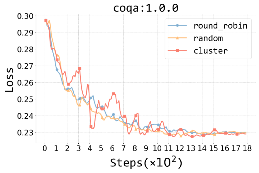
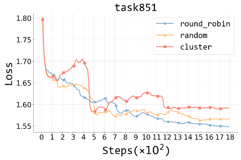
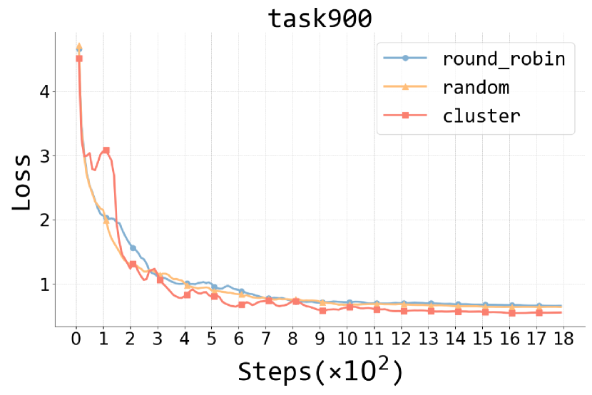
Figure 2: Sudden decrease in the average loss under cluster scheduling for the three tasks at steps 400, 450, and 150 respectively.

We have demonstrated that zero-shot generalization occurs at the early stage during instruction tuning. However, the reasons why models can achieve noteworthy generalization during this phase await investigation. The model receives only a limited amount of supervised data during this phase. Therefore, despite the scarcity, these data ought to play a significant role in facilitating generalization. With this intuition, we investigate the impact of exposure to different training data permutations during the early stage of instruction tuning.

Data and Settings. We apply 1600 Flan-mini training tasks to get a series of instruction-tuned checkpoints and evaluate them on various Flan-mini unseen tasks. Please refer to Section B.1 for more details. Specifically, we examine the following three training data permutations:

• Round-robin: We employ round-robin scheduling to disperse training tasks as much as possible. Consequently, the model iterates over one data point from each task every 100 training steps.

• Cluster: We arrange all data from each task together, resulting in task-level clusters throughout the entire training dataset. Consequently, the model trains on 8 new tasks every 10 steps.

• Random: We randomly shuffle all training data as a baseline for comparison.

Results. Different training data permutations entail different loss curve patterns. As shown in Figure 2, the pattern of random and round-robin scheduling is similar due to round-robin being an extreme form of data shuffling. However, cluster scheduling differs largely from both. At certain steps during the instruction tuning, there exists a sudden decrease in average loss across different test tasks. This further highlights that leveraging a relatively small amount of data may induce a substantial drop in the average loss, thus causing a great impact on zero-shot generalization.

3.2 Zero-Shot Generalization through Data Similarity and Granularity

We have observed that training data permutation could lead to significant changes in the loss curve and that the timing of presence for certain data may greatly facilitate generalization on unseen tasks. With these findings, we naturally ask what is the best permutation that facilitates zero-shot generalization the most, and how to arrange these “certain data” that promote early generalization. In the following sections, we seek to address these questions through two perspectives: similarity and granularity.

3.2.1 Enhancing Zero-Shot Generalization through High-Similarity Data

Previous research [9, 50] has consistently demonstrated that the performance of downstream tasks improves when the similarity between the pre-training data and the downstream task data increases. This finding aligns with our intuitive understanding that data points with higher similarity can better facilitate generalization. Furthermore, we have observed that zero-shot generalization consistently occurs during the early stages of instruction tuning. Based on these insights, we propose and subsequently validate that: [couleur= msftBlack!05, epBord=1, arrondi=0.1, logo=, marge=6, ombre=true, blur, couleurBord=msftBlack!10, tailleOndu=2, sousTitre =Takeaway 3: Encountering data with high similarity early during instruction tuning will greatly enhance zero-shot generalization compared to encountering such data later.]

Selection of Similarity Measures. To validate our hypothesis, we first have to define how to measure the similarity. To effectively permute all the training data, we aim to calculate the similarity distance between each training data point and the whole test set. Specifically, we investigate two main categories of similarity measures:

• N-gram similarity: We respectively measure the similarity distance by calculating the KL divergence between the bigram word distributions of each training set data point and all the test set data.

• Embedding similarity: We utilize all-MiniLM-L6-v2  from Sentence Transformer [36] to compute embeddings for each training and test data and then calculate the Cosine and Euclidean similarity distances, as detailed in Section B.3. Next, we refer to four classical distance calculation methods , namely “max” (maximal distance), “min” (minimal distance), “avg” (unweighted average distance), and “centroid” (centroid distance), to represent the distance of each training set data point to all the test set data.

We analyze a series of instruction-tuned checkpoints on Flan-mini and calculate the similarity distance between the training data seen by the $k^{th}$ checkpoint and all the test data. This entails in total nine similarity calculation methods ({N-gram} + {Cosine, Euclidean} $\times$ {max, min, avg, centroid}). Please refer to Section B.3 for exact calculation methods. Through analyzing LABEL:fig:nine_similarity_with_loss, we find that i) cosine and Euclidean measures show little difference; ii) the drop in minimum distance calculation coincides with the drop in loss curve; iii) average distance calculation promotes fairness by involving all test data in the actual calculation. Therefore, we consider using the Cosine Average (Cosine-Avg) and Cosine Minimum (Cosine-Min) for similarity calculation in later experiments. We also prove they both satisfy optimal substructure, ensuring that the effect of training set permutation according to Cosine-Avg or Cosine-Min can accumulate over time as more data point is presented to the model, detailed in Section B.5

Introduction of Weighted Similarity Distance. To raise the stability of computation and leverage the strengths from both Cosine-Avg and Cosine-Min, we consider performing a simple linear combination of both metrics for real similarity calculation. We denote our similarity distance measurement as Weighted Similarity Distance (WSD). Specifically, for each training data point $x_{i}$, we assume that the Average Distance and the Minimum Distance from $x_{i}$ to $\mathcal{D}_{\text{Test}}$ are $\text{AD}_{i}$ and $\text{MD}_{i}$ respectively. We define our WSD measure as follows:

$$\text{WSD}_{i}=w_{\text{avg}}\text{AD}_{i}+w_{\text{min}}\text{MD}_{i}$$ (1)

Empirically, we set $w_{\text{avg}}=1$, and $w_{\text{min}}$ to a scaling factor to ensure Cosine-Avg and Cosine-Min have the same magnitude, detailed in Equation 14. We investigate the impact of the WSD on zero-shot generalization during instruction tuning. Specifically, we examine three training permutations: Nearest First Training (NFT), Farthest First Training (FFT), and Random Training (RT) on the multi-task dataset Flan-mini. This setup allows us to differentiate between the nearest and farthest data points in terms of the temporal dimension of instruction tuning. By evaluating a series of fine-grained saved instruction-tuned checkpoints, we can compare the effects of the three settings and gain a clear understanding of the impact of WSD-based premutation on zero-shot generalization. More details are illustrated in Section B.1.

Settings. We utilize the Flan-mini dataset and randomly sample up to 20 instances for each training task. Each test task consists of at most five test data points to form a test set. We permute the training data based on the WSD measure to create the NFT, FFT, and RT settings. For each setting, we perform instruction tuning on the three training data permutations, resulting in a series of fine-grained checkpoints. We then calculate the average loss for each checkpoint on the test set containing various test tasks.

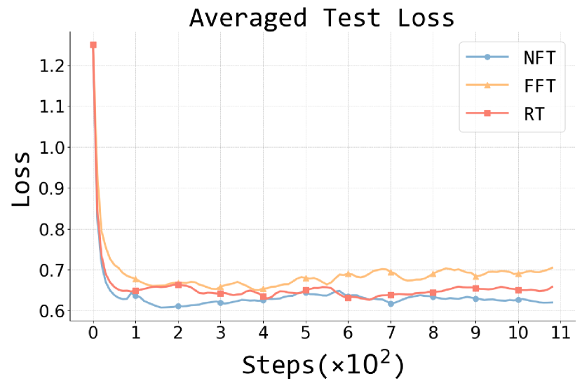
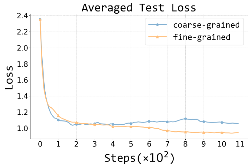
Figure 3: Left: The impact of the three similarity settings (NFT, FFT, and RT) on averaged test loss. Right: The impact of different granularity settings on averaged test loss.

Results. The earlier the model encounters data with high similarity to the test set, the more beneficial it is for zero-shot generalization. As shown in the left plot of Figure 3, we can observe that the NFT setting exhibits a rapid and low loss reduction, indicating better zero-shot generalization. In contrast, the FFT setting shows relatively poorer zero-shot generalization compared to the baseline RT setting.

3.2.2 Enhancing Zero-Shot Generalization through Fine-Grained Data

Traditional methods to enhance zero-shot generalization are mostly confined to the task level, focusing on task-pair transfer. However, the so-called “tasks” or “categories” are artificially defined and, from the perspective of LLMs, they are merely a collection of tokens or embedding representations. Therefore, different “tasks” or “categories” may still appear relatively similar to LLMs, while instances from the same task may exhibit profound differences. Thus, we propose and validate that:

[couleur= msftBlack!05, epBord=1, arrondi=0.1, logo=, marge=6, ombre=true, blur, couleurBord=msftBlack!10, tailleOndu=2, sousTitre =Takeaway 4: Treating all data points equally in finer granularity without the concept of “task” as constraints better promotes zero-shot generalization.]

Settings. We use the Flan-mini dataset and randomly sample up to 20 instances for each training task. We employ two approaches to permute the training data: i) coarse-grained setting, where all instances under each training task are clustered and then shuffled. We define the embedding of a task as the average embedding of all instances under that task. ii) fine-grained setting, where all data instances are directly shuffled instead of first being clustered.

Results. Compared to the coarse-grained setting, the fine-grained setting is more beneficial for enhancing zero-shot generalization. As shown in the right plot of Figure 3, the loss curve for the fine-grained setting decreases more quickly and effectively, indicating that removing task framework constraints can further improve zero-shot generalization.

4 Understanding Zero-Shot Generalization

In previous experiments, we empirically apply Cosine-Avg and Cosine-Min, as well as the WSD measure obtained through weighting. However, these measures inherently possess shortcomings: i) Cosine-Avg cannot distinguish the variance within the test set. When the test set collapses to the point where all data points are the same, the distribution becomes a spike; when the test set data is sufficiently spread out, the distribution becomes uniform. In both cases, the Cosine-Avg distance from all test data points to a certain training data point remains consistent, indicating that it could not distinguish the role of each test data point. ii) Cosine-Min cannot holistically represent all test set data points. If a certain test data point is closer to all training data points than all other test data points, Cosine-Min only considers the distance to that test data point and does not take into account others, even if they are relatively far away.

Therefore, we seek an approach that can better distinguish and permute the training data for enhanced zero-shot generalization. To this end, we present the Test-centric Multi-turn Arrangement (TMA).

Algorithm 1 Test-centric Multi-turn Arrangement Method

1:Dataset $\mathcal{D}$ split into training set $\mathcal{D}_{\text{train}}$ and test set $\mathcal{D}_{\text{test}}$

2:Sub-training sets $\mathcal{D}_{\text{train}}^{i}$ for each round $i$

3:$i\leftarrow 0$

4:while $\mathcal{D}_{\text{train}}\neq\emptyset$ do

5:     $i\leftarrow i+1$

6:     $\mathcal{D}_{\text{train}}^{i}\leftarrow\emptyset$

7:     for all $x\in\mathcal{D}_{\text{test}}$ do

8:         Find the nearest data point $y\in\mathcal{D}_{\text{train}}$ to $x$ based on cosine similarity

9:         $\mathcal{D}_{\text{train}}^{i}\leftarrow\mathcal{D}_{\text{train}}^{i}\cup\{y\}$

10:     end for

11:     $\mathcal{D}_{\text{train}}\leftarrow\mathcal{D}_{\text{train}}\setminus\mathcal{D}_{\text{train}}^{i}$

12:end while

13:return $\mathcal{Q}_{\text{train}}=\{\mathcal{D}_{\text{train}}^{1},\mathcal{D}_{\text{train}}^{2},\ldots,\mathcal{D}_{\text{train}}^{k}\}$

Formalization. We formalize TMA algorithm in Algorithm 1. This arrangement of the training data ensures that the embedding of each test data point is equally considered, thus taking into account all their characteristics. It avoids the limitations of Cosine-Avg, which disregards the distribution within the test data, or Cosine-Min, which only considers individual test data embeddings. A more detailed investigation of our arrangement method is provided in Section C.4.

4.1 Test-centric Multi-turn Arrangement Enhances Zero-Shot Generalization

With all the nice properties presented by TMA, we show that: [couleur= msftBlack!05, epBord=1, arrondi=0.1, logo=, marge=6, ombre=true, blur, couleurBord=msftBlack!10, tailleOndu=2, sousTitre =Takeaway 5: Test-centric Multi-turn Arrangement can further enhance zero-shot generalization, regardless of whether the data source involves the concept of “task” or not.]

Data and Settings. We employ two types of datasets: i) datasets with task splits, such as Flan-mini [14], and ii) datasets without task splits, such as ShareGPT [46] and NoRobots [35]. Flan-mini consists of task-specific splits, while ShareGPT and NoRobots are general dialogue datasets. We arrange the training data by applying Algorithm 1 and examine the same three training permutations, namely NFT, FFT, and RT, which are consistent with the experimental setup described in Section 3.2.1. Specifically, NFT under this setting refers to the sequential training data order as returned by Algorithm 1, and FFT refers to its reverse. For detailed configurations, please refer to Section C.2.

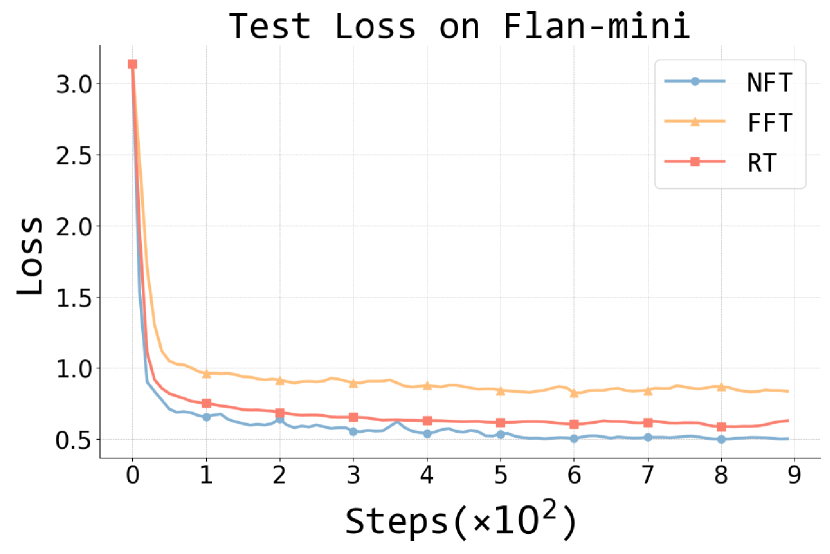
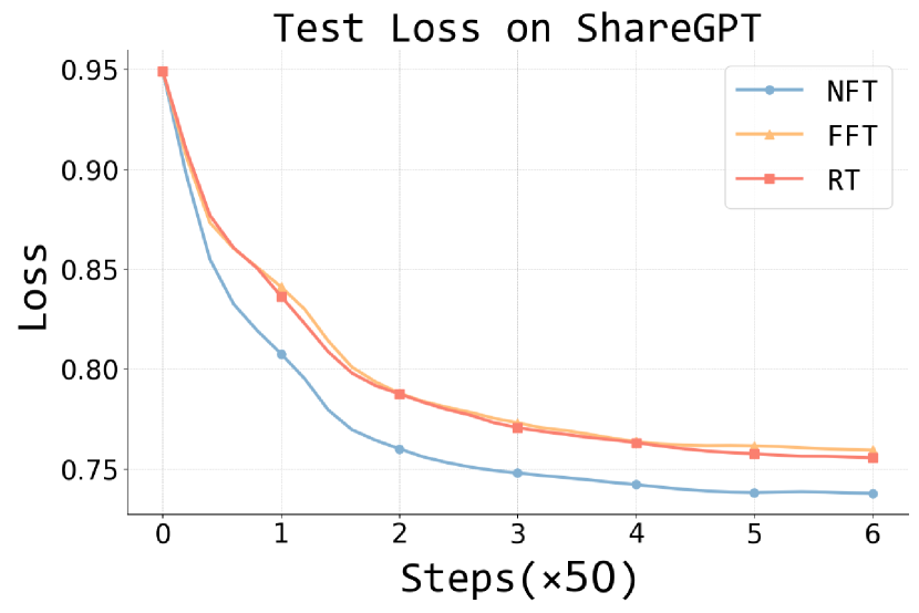
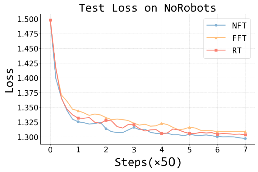
Figure 4: Averaged test loss of three similarity settings (NFT, FFT, and RT) under Test-centric Multi-turn Arrangement on Flan-mini (left), ShareGPT (middle), and NoRobots (right).

Results. Using the Test-centric Multi-turn Arrangement to order training data from nearest to farthest significantly enhances zero-shot generalization. As illustrated in Figure 4, whether with the task split in Flan-mini (left) or without the task split in ShareGPT (middle) and NoRobots (right), the loss curve under the NFT setting decreases more rapidly while reaching a lower point, whereas the FFT setting results in the poorest performance. This further validates the effectiveness of our arrangement method. We also conduct an ablation study on the final distribution of $\mathcal{Q}_{\text{train}}$, as detailed in Section C.3. We reveal that accessing high-similarity data during instruction tuning can facilitate continual learning and further loss reduction.

4.2 Early-Selected Sub-Training Set Shows Higher Effectiveness

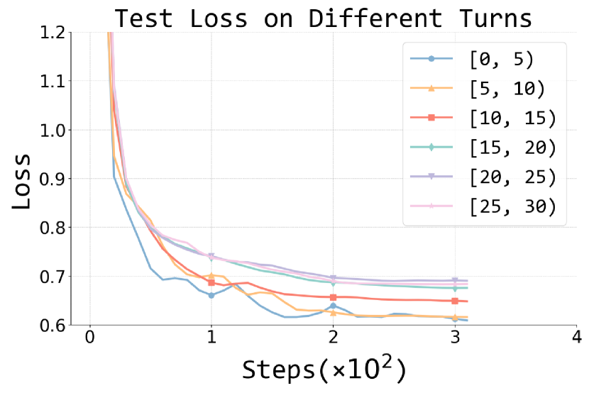
Figure 5: Averaged test loss on different turns of training data.

The final training set $\mathcal{Q}_{\text{train}}$ in the TMA algorithm is formed through multiple rounds of selections in order. We show that: [couleur= msftBlack!05, epBord=1, arrondi=0.1, logo=, marge=6, ombre=true, blur, couleurBord=msftBlack!10, tailleOndu=2, sousTitre =Takeaway 6: The earlier the sub-training set selected by TMA, the better its effect in promoting zero-shot generalization.]

Data and Settings. We apply Flan-mini as in the previous experiment. Specifically, we cluster the training data selected from rounds $[i,i+5)(i=0,5,10,15,20,25)$ based on TMA, and respectively perform instruction tuning. Then, for each instruction-tuned checkpoint, we calculate the average loss on the test set.

Results. The training data selected from the earliest rounds generally exhibits higher quality. As shown in Figure 5, we observe that from rounds $[0,5)$ to $[25,30)$, the decrease in loss becomes slower, and the minimum loss value tends to be higher. This indicates that our arrangement method could successfully distinguish high-quality training data and apply them early in tuning to enhance zero-shot generalization.

5 Related Work

In the course of deep learning’s development, several intriguing training dynamics have gradually been discovered, such as grokking [29], double descent [1], emergent abilities [49], and zero-shot generalization on unseen tasks. The first three phenomena have already received substantial explanations. For grokking, it happens from algorithm tasks [29] to a broader spectrum of realistic tasks [23], explained through the Slingshot Effects [42] or the competition between memorization and generalization circuits [44]. For double descent, Nakkiran et al. [27] proposed that double descent occurs both model-wise and epoch-wise, while Davies et al. [10] unified grokking and double descent through the learning speed and generalization ability of patterns. Regarding emergent abilities, Schaeffer et al.[38] suggested that the occurrence of emergent abilities is due to researchers using non-smooth metrics. Hu et al.[18] extended this idea by proposing an infinite resolution evaluation to predict the emergence of abilities, and Du et al. [12] attempted to understand emergent abilities from the perspective of loss. In the rapid development of LLMs, security issues have increasingly attracted the attention of researchers [8, 57]. Solving these security challenges relies on an in-depth understanding of training dynamics, which is crucial for comprehending the mechanisms of neural networks and contributes to building robust and interpretable LLMs. Research on these dynamics also offers valuable insights for investigating zero-shot generalization, especially the work on emergent abilities. We suggest that model-wise emergent abilities may be analogous to step-wise zero-shot generalization.

LLMs have been proven capable of zero-shot generalization across a variety of downstream tasks [2], and instruction tuning has emerged as the most effective method to achieve this [5, 37, 48]. Instruction-tuned LLMs possess strong capabilities in instruction following and logical reasoning. Moreover, enhancing their understanding of the implicit intentions behind instructions [31] makes it possible to develop these models into powerful agents [30, 34, 32, 33]. The zero-shot generalization phenomenon resulting from instruction tuning is crucial for building general LLMs. This means that models trained on certain tasks can generalize well to unseen tasks. Multi-task datasets designed for this purpose have continuously iterated in quality, quantity, and diversity, and numerous studies have explored how zero-shot generalization occurs during the instruction tuning process. Sanh et al. [37] constructed P3 using explicit multitask learning, demonstrating that explicit task prompt templates can promote zero-shot generalization. Wang et al. [47] created the Super Natural Instructions V2 (NIV2) dataset, which comprises over 1600 task types, and empirically showed that more observed tasks, an adequate number of training instances, and larger models improve generalization. Meta introduced OPT-IML [19], investigating the impacts of dataset scale and diversity, different task sampling strategies, and the presence of demonstrations on generalization. Subsequently, Chung et al. [24] proposed the Flan Collection, which encompasses up to 1836 tasks, and pointed out that scaling the number of tasks and model size, as well as incorporating chain-of-thought data, can dramatically improve performance on unseen tasks.

In addition, a line of research focuses on understanding the relationships in task-pair transfer [40, 45, 52], suggesting that not all tasks contribute positively to zero-shot generalization; some tasks may even result in negative transfer effects [21, 26, 56]. However, a significant limitation of the aforementioned works is that, whether training on one task and then evaluating on another [21, 56], or simply calculating intermediate task [45] or instruction [22] transfer scores, all these efforts to select the most informative tasks to promote zero-shot generalization are confined within the “task” framework. This approach is based on a premise: the human-defined “tasks” and even “categories” are sufficiently reasonable. This is precisely the issue our study strives to address: breaking free from the task-level framework to explore “generalization” at a more fundamental level.

6 Conclusion

Our research sheds light on the mechanism underlying zero-shot generalization during instruction tuning, moving beyond the conventional task-level analysis to a more data-centric perspective. By demonstrating that zero-shot generalization occurs early during instruction tuning and is significantly influenced by data similarity and granularity, we provide a new understanding of how instruction tuning brings up zero-shot generalization. Our proposed Test-centric Multi-turn Arrangement further illustrates the importance of accessing high-similarity data early in the training process to facilitate continual learning and loss reduction. For future work, we suggest exploring the quantitative relationship between similarity distance and loss. Specifically, investigating whether similarity distance can predict a model’s generalization performance on new data could further help the optimization of instruction tuning. We hope our findings will pave the way for developing more aligned and robust LLMs, enhancing their ability to generalize effectively in diverse applications.

Appendix

Appendix A Details for Section 2

A.1 Data and Setting

We utilized three datasets: Super Natural Instructions V2 [47], Public Pool of Prompts [37] and Flan-mini [14]. Here, we provide a detailed overview of each dataset.

NIV2.

Super Natural Instructions V2 (NIV2) is a large collection of tasks and their natural language definitions/instructions, with 746 tasks comprising a total of 74,317 instances in train split. In the NIV2 dataset, each task is characterized by its task name, task definition, positive examples, negative examples, and explanations, accompanied by several task instances comprising input and output. We adopt the default configuration in NIV2 repository , as illustrated in Table 1.

# Instances Per Task	# Instances Per Eval Task	Add Task Name	Add Task Definition	# Pos/Neg Examples	Add Explanation	Tk Instruct
100	100	False	True	2/0	False	False

Table 1: The hyper-parameters applied in NIV2 configuration.

P3.

Public Pool of Prompts (P3) is a collection of prompted English datasets covering a diverse set of NLP tasks. It is organized into a three-level hierarchy of category, task, and prompt template. For each task, instances are organized into a group of data according to several prompt templates. We refer to such binary pairs of (task, prompt) as a base-class dataset. We utilize the same base-class datasets for training and evaluation as we did for training and evaluating vanilla T0 . In the end, we filter out 284 training base-class datasets and 123 evaluation base-class datasets. Due to the vast amount of the P3 dataset and preliminary experiments indicating early zero-shot generalization, for each training base-class dataset, we randomly select up to 100 instances, resulting in a total of 28,372 training instances.

Flan-mini.

The flan-mini dataset is a carefully selected subset maintaining a high level of task diversity while reducing the overall FLAN collection size, encompassing not only the Flan2021 Collection and P3 data but also various ChatGPT datasets, including Alpaca, Code Alpaca, and ShareGPT, significantly increasing the diversity of tasks in the flan-mini dataset. In total, there are 1825 tasks, with 1600 tasks allocated for training and 225 unseen tasks for evaluation. Due to the vast amount of training data and preliminary experiments indicating early zero-shot generalization, we randomly select up to 20 instances for each training task, resulting in a total of 28,751 training instances.

A.2 Training Template and Examples

Concatenating the various fields from the data, examples of complete training data appear as follows:

  NIV2 example

⬇

<s>User: Definition: In this task, you will be shown a sentence, and you should determine whether it is overruling or non-overruling. In law, an overruling sentence is a statement that nullifies a previous case decision as a precedent by a constitutionally valid statute or a decision by the same or higher ranking court which establishes a different rule on the point of law involved. classify your answers into overruling or non-overruling.

Positive Example 1 -

Input: 876 f.3d at 1306.

Output: non-overruling.

Positive Example 2 -

Input: we disapprove cooper and craven to the extent that they may be read to conflict.

Output: overruling.

Now complete the following example -

Input: the court’s discussion fails to adequately account for the origin of the specific intent element that both section 2(a) and 2(b) contain.

Output:

Assistant: non-overruling.</s>

  P3 example

⬇

<s>User: I took part in a little mini production of this when I was a bout 8 at school and my mum bought the video for me. I’ve loved it ever since!! When I was younger, it was the songs and spectacular dance sequences that I enjoyed but since I’ve watched it when I got older, I appreciate more the fantastic acting and character portrayal. Oliver Reed and Ron Moody were brilliant. I can’t imagine anyone else playing Bill Sykes or Fagin. Shani Wallis’ Nancy if the best character for me. She put up with so much for those boys, I think she’s such a strong character and her final scene when... Well, you know... Always makes me cry! Best musical in my opinion of all time. It’s lasted all this time, it will live on for many more years to come! 11/10!! How does the reviewer feel about the movie?

Assistant: They loved it</s>

  Flan-mini example

⬇

<s>User: Do these sentences have the same meaning?

" The bank requires growth from elsewhere in the economy and needs the economy to rebalance , " he said in an interview with the Press Association news agency .

The Bank of England " requires growth from elsewhere in the economy and needs the economy to rebalance , " he told the Press Association news agency .

Available options:

(1). no;

(2). yes;

Assistant: (2).</s>

A.3 Hyper-Parameter Details

Model	Max Length	Epochs	BS Per Device	LR	Save Steps	LR Scheduler	Optimizer
LLaMA-2-7B	1024	1	8	1e-06	10	Cosine	AdamOffload

Table 2: The hyper-parameters applied during the instruction tuning. LR denotes the learning rate and BS denotes the batch size.

For instruction tuning, we present some key hyper-parameters related to instruction tuning in Table 2. Additionally, we utilize the model-center framework [25] to conduct full-parameter instruction tuning of LLaMA-2-7B on two 80GB A800s and dynamically adjust the loss scale based on the changing training loss to prevent underflow. All of our instruction tuning experiments utilize these hyper-parameters consistently.

Model	Max Gen Length	Repetition Penalty	Batch Size	Top-p	Temperature
LLaMA-2-7B	128	1.2	8	0.9	0.9

Table 3: The hyper-parameters applied during the generation.

For generation, we present some key hyper-parameters during the generation in Table 3. We still employ the model-center framework to conduct the generation of LLaMA-2-7B on one 80GB A800. All of our generations utilize the aforementioned hyper-parameters consistently.

A.4 Evaluation Details

Instruction-tuned model as a generalist.

Initially, we evaluate the model’s generalization ability at a holistic level, termed as a generalist. To achieve this, we randomly select 120 samples from all testing data, including a series of unseen tasks. These samples are evaluated against a series of fine-grained checkpoints saved during the instruction tuning stage. The average scores for Loss, ROUGE-1, ROUGE-L, RM Score, and Exact-Match across all samples are calculated. We present the calculation details and formulas of each metric above.

• Loss: We use cross entropy to calculate the error between labels and predictions. Because the position with a value of -100 in labels is a padding position, we ignore the prediction at this position during calculation.

• ROUGE-1: ROUGE-1 measures the comprehensiveness of the generated summary by calculating the overlap between words in the generated summary and words in the reference summary:

  $$\text{ROUGE}\textnormal{-}1=\frac{\text{Number of overlapping unigrams}}{\text{Total number of unigrams in reference summary}}$$ (2)

• ROUGE-L: ROUGE-L is based on the idea of Longest Common Subsequence (LCS). By measuring the length $m$ of the reference summary $X$ and the length $n$ of the generated summary $Y$, the ROUGE-L score is calculated as follows:

  $$R_{lcs}=\frac{\operatorname{LCS}(X,Y)}{m}$$ (3)

  $$P_{lcs}=\frac{\operatorname{LCS}(X,Y)}{n}$$ (4)

  $$F_{lcs}=\frac{\left(1+\beta^{2}\right)R_{lcs}P_{lcs}}{R_{lcs}+\beta^{2}P_{lcs}}$$ (5)

• Exact-Match: First of all, we normalize the answers by removing extra spaces, removing punctuation, and converting all characters to lowercase. Then, for each question-answer pair, if the characters of the model’s prediction exactly match the characters of the true answer, EM = 1, otherwise EM = 0. This is a strict all-or-nothing metric; being off by a single character results in a score of 0.

  $$\text{EM}=\begin{cases}1&\text{if the model's prediction exactly matches the true answer}\\ 0&\text{otherwise}\end{cases}$$ (6)

• RM score: Let $S$ represent the sentence to be evaluated, $f$ is the reward model function, which takes as input the sentence $S$ and model parameters $\theta$. We use UltraRM-13B as the reward model. Formally, the RM score assigned to sentence $S$ is defined as:

  $$R(S)=f(S,\theta)$$ (7)

	NIV2			P3			Flan-mini
	Train	General Eval	Speical Eval	Train	General Eval	Speical Eval	Train	General Eval	Speical Eval
# Tasks	746	—	119	284	—	123	1600	—	225
# Instances	74317	120	595	28372	120	—	28751	120	1121

Table 4: Detailed statistics for train and test splits of NIV2, P3, and flan-mini in our experiments. General Eval denotes the evaluation as a generalist. Special Eval denotes the evaluation as a specialist.

Instruction-tuned model as a specialist.

In order to facilitate more granular research on task-level scenarios, i.e., exploring the model’s generalization ability on specific unseen tasks, termed as a specialist, we take NIV2 and flan-mini datasets as examples. For each unseen task, we randomly select up to five testing instances. As shown in  Table 4, for evaluation as a specialist, the flan-mini test set comprises a total of 1,121 instances, covering all 225 unseen tasks. Additionally, the NIV2 test set contains a total of 595 instances, covering all 119 unseen tasks.

Subsequently, we allow a series of fine-grained checkpoints to generate answers on these 1,121 testing instances and compute the loss. We define the generalization metric on a specific unseen task as the average loss of up to five testing instances for that task, to verify whether the model specializes in it.

A.5 Discussion for Metrics

In previous experiments, we have discovered that zero-shot generalization might occur early in the instruction tuning process based on the ROUGE series, Exact-Match, and RM score. However, these metrics may not be suitable for measuring generalization effectively. First, for the ROUGE series, ROUGE-1 refers to the overlap of unigrams, and ROUGE-L is based on the longest common subsequence. Both metrics are limited to surface-level matching, primarily relying on lexical overlap between model outputs and labels, to the extent that capturing semantic similarity or a deeper understanding of the content conveyed in the sentences becomes challenging [13, 15]. Outputs and labels with different wordings but similar meanings may receive low ROUGE scores.

While the reliability of ROUGE series scores is questionable, metrics like Exact-Match are nonlinear, and previous research [38] has shown that nonlinear metrics are prone to observing emergent abilities. Although emergence is a model-wise phenomenon, if we adopt such nonlinear metrics step-wise, i.e., along the training timeline, we might also observe step-wise “emergence” so-called generalization phenomena. This might lead to misjudgments regarding the timing of zero-shot generalization. Therefore, we need to address this issue.

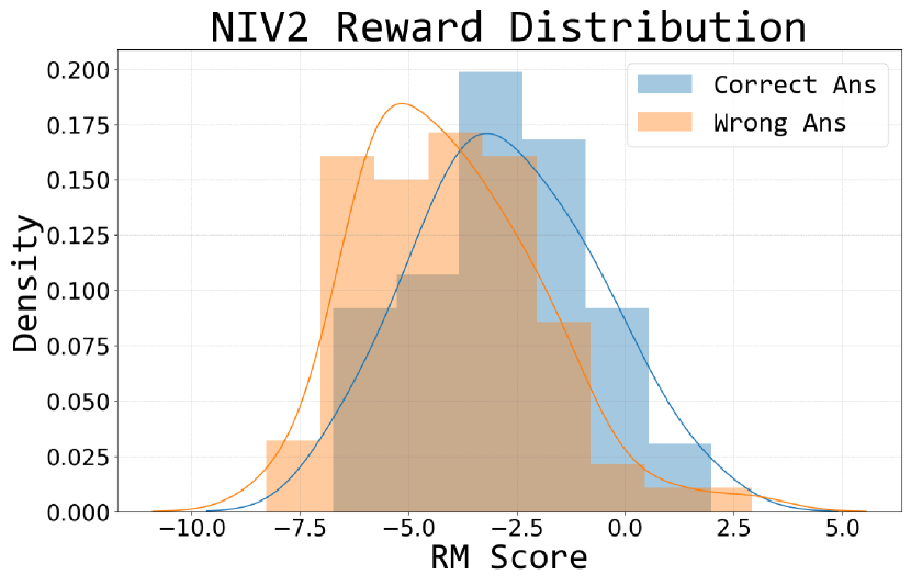
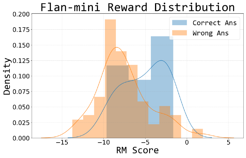
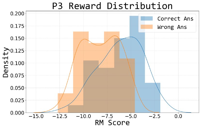
Figure 6: The reward distribution regarding the answer’s correctness on NIV2 (left), Flan-mini (middle), and P3 (right). The area under both curves in each figure has large overlaps, indicating the reward cannot well distinguish the quality of answers.

Acknowledging that the Reward Model (RM) is trained on preference data, it is inevitable that there will be a certain loss of ability when generalizing to out-of-distribution (OOD) datasets [39]. Consequently, scoring on different datasets may not be precise. As shown in Figure 1, RM scores for NIV2 are notably higher than those for the other two datasets, indicating a bias. Further, we compare the reward distribution with respect to the correctness of the model response respectively on the three datasets. The large overlap under both curves in Figure 6 indicates that RM could not well distinguish between responses of lower or higher quality. This further highlights the inappropriateness of using RM score to reflect zero-shot generalization.

A.6 Case Study

Continuing our investigation, we further delve into the fine-grained analysis of the generalization capability on individual unseen tasks.

Settings

Taking NIV2 and Flan-mini as examples, we curate a maximum of five test data points for each unseen task, consolidating them into a single test set. Similarly, we generate outputs using a series of fine-grained instruction-tuned checkpoints and compute the cross-entropy loss against the labels and average on a per-task level. For detailed evaluation settings, please refer to Section A.4.

Results.

From the perspective of individual unseen tasks, zero-shot generalization also occurs in the early stage of instruction tuning. However, different tasks exhibit distinct trends in terms of zero-shot generalization. We identified two primary trends: rapid decrease followed by stability and sharp decline followed by a gradual decrease, as shown in LABEL:fig:loss_classfied_figures. This finding further suggests that the majority of unseen tasks are generalized in the early stage of instruction tuning.

Appendix B Details for Section 3

B.1 Different Training Distributions

In Section 3, we take the Flan-mini dataset as an example. For each training task, we select a maximum of 20 data points, and for each testing task, we select a maximum of 5 data points. We employed various training data distributions on Flan-mini. Here, we provide detailed explanations of the data permutation methods and training specifics.

• Round-robin: In the round-robin setting, with a total batch size of 16, we save checkpoints every 10 steps during instruction tuning. Hence, there is a difference of 160 training data points between adjacent checkpoints. Considering the Flan-mini dataset, where we have divided 1600 training tasks, it takes 1600 data points to traverse all training tasks. Therefore, for every 10 checkpoints (every 100 steps), the model completes one pass over all training tasks.

• Cluster: In the cluster setting, similarly, there is a difference of 160 training data points between adjacent checkpoints. However, for each training task, we curate a maximum of 20 data points. Consequently, between adjacent checkpoints, the model encounters almost exactly 8 tasks.

• RT (Random Training): As a baseline, we randomly shuffle all training data.

• NFT (Nearest First Training): Given a certain similarity distance measure such as Weighted Similarity Distance (WSD), we compute the similarity distance from each training data point to the test set based on this measure, and then permute the training data points from nearest to farthest.

• FFT (Farthest First Training): Given a certain similarity distance measure such as Weighted Similarity Distance (WSD), we calculate the similarity distance from each training data point to the test set based on this measure, and then permute the training data points from farthest to nearest.

B.2 Effect of Test Data Distributions

Upon discovering that controlling the permutation of training data leads to entirely different loss curves for unseen tasks, we next aim to explore the impact of test data distribution on the results. As the order of test data does not impact the valuation results, we sample test data by employing different seeds to obtain varying test data subsets from the same task. Subsequently, we generate and calculate average loss across a series of fine-grained instruction-tuned checkpoints.

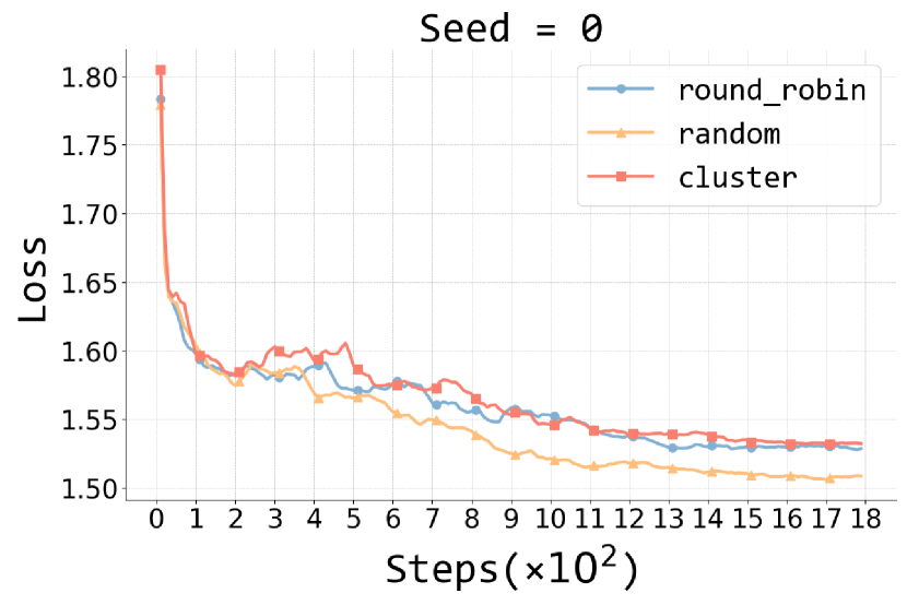
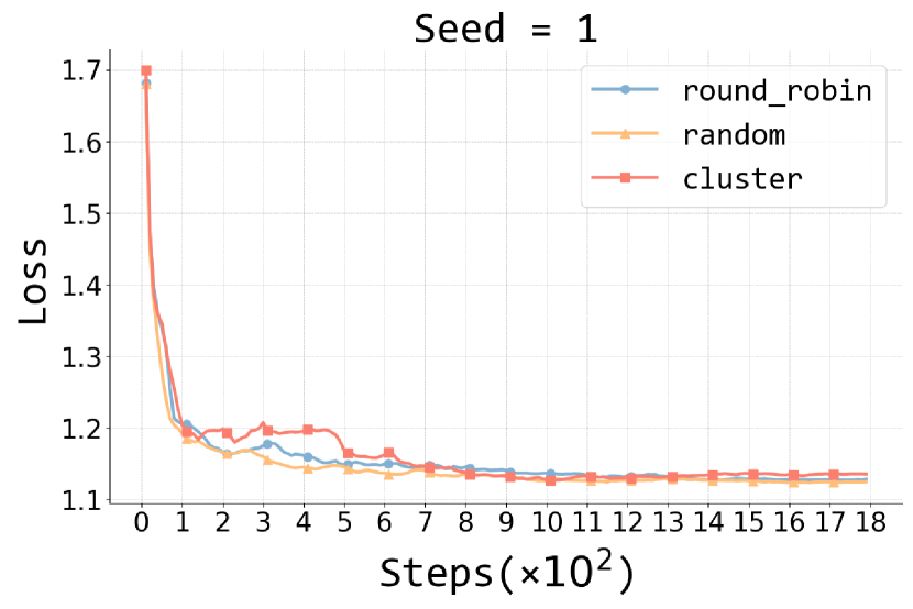
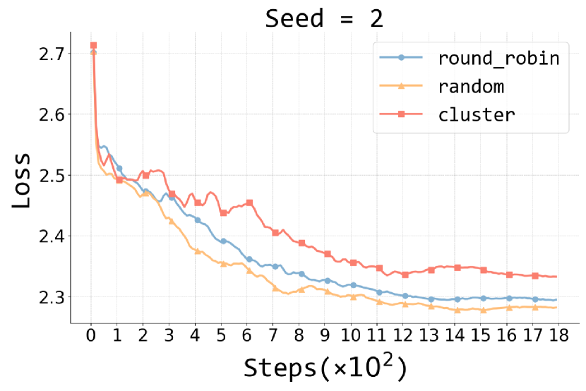
Figure 7: The descent in loss transitions from being gradual ($seed=2$) to rapid ($seed=0/1$). (task1264_ted_translation_pl_pt)

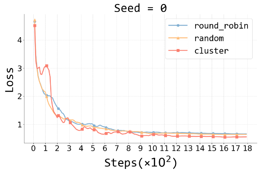
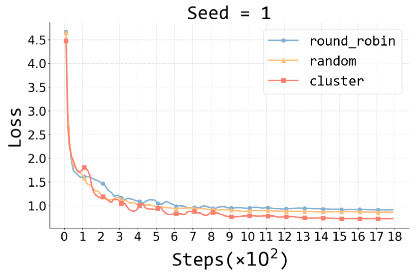
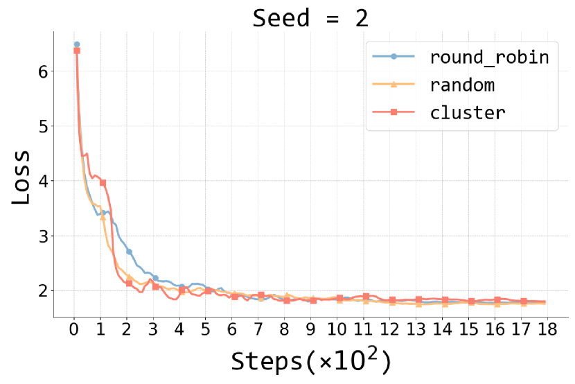
Figure 8: The sudden decrease ($seed=0/2$) observed in cluster scheduling disappears ($seed=1$). (task900_freebase_qa_category_classification)

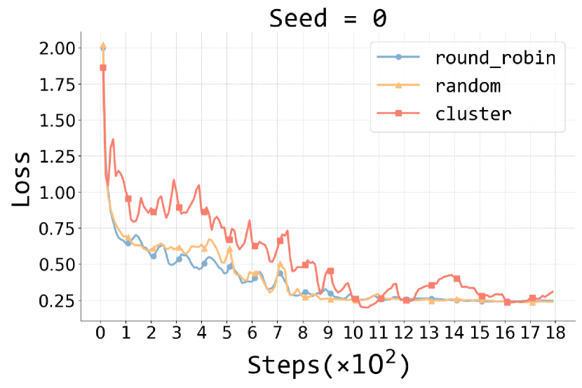
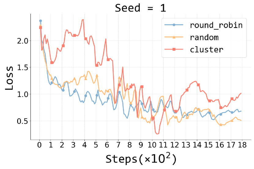
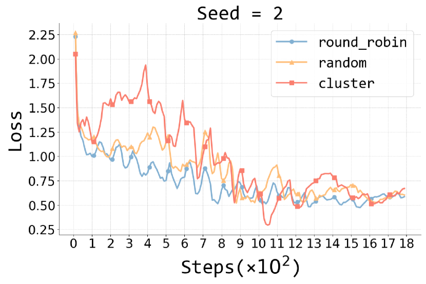
Figure 9: The fluctuation ($seed=1/2$) in loss becomes more stable ($seed=0$). (task050_multirc_answerability)

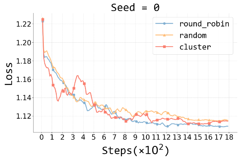
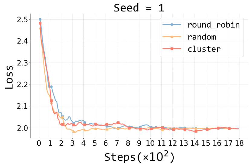
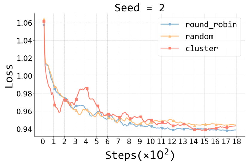
Figure 10: The lowest point of loss shows a significant decrease (from $seed=1$ to $seed=0/2$). (task511_reddit_tifu_long_text_summarization)

Under different seeds, which represent different subsets of test data for the same task, we observed that the loss curves exhibit distinct patterns:

• The descent in loss transitions from being gradual to rapid (Figure 7).

• The sudden decrease observed in cluster scheduling disappears (Figure 8).

• The fluctuation in loss becomes more stable (Figure 9).

• The lowest point of loss shows a significant decrease (Figure 10).

B.3 Similarity Measure Details

B.3.1 Embedding-based Similarity Measure

We utilize all-MiniLM-L6-v2  as our embedding model, which maps sentences to a 384-dimensional dense vector space. When generating the embedding vector of a particular piece of data, we simply format the instruction and answer of this data into a template like “{instruction} {answer}”, and then put this whole string into the embedding model to generate the corresponding embedding. After obtaining the embedding of each data, we compute the similarity distance between a training and a test data in the following two ways:

• Cosine similarity distance: Cosine similarity determines the similarity by computing the cosine of the angle between the two embeddings, yielding a value between -1 and 1. A value closer to 1 indicates higher similarity, while a value closer to -1 indicates lower similarity. When calculating, we add a negative sign to the cosine similarity to indicate the distance. Thus, a larger value indicates a greater distance between two embeddings. Suppose $\mathbf{A}$ and $\mathbf{B}$ are two embeddings, “$\cdot$” denotes the dot product of the embedding vectors, and $\|\mathbf{A}\|$ and $\|\mathbf{B}\|$ represent the L2 norms of the embeddings. We calculate the cosine similarity distance as follows:

  $$\text{cosine\_similarity\_distance}=\frac{{\mathbf{-A}\cdot\mathbf{B}}}{{\|\mathbf{A}\|\cdot\|\mathbf{B}\|}}$$ (8)

• Euclidean similarity distance: This method calculates the straight-line distance between two points in space. A higher distance value indicates a farther distance between the two embeddings. The Euclidean distance between two points $\mathbf{A}$ and $\mathbf{B}$ in an $n$-dimensional space is computed using the formula:

  $$\text{Euclidean\_similarity\_distance}=\sqrt{\sum_{i=1}^{n}(A_{i}-B_{i})^{2}}$$ (9)

Assuming that we have $N_{\text{train}}$ training data and $N_{\text{test}}^{T}$ test data (for an unseen task $T$), we calculate a similarity distance matrix $D$ with shape $(N_{\text{train}},N_{\text{test}}^{T})$, where each entry $d_{ij}$ represents the cosine or Euclidean similarity distance between the $i^{th}$ training data and the $j^{th}$ test data. For the ${k^{th}}$ saved checkpoints, it has seen $160\times k$ training data, so the Similarity Distance $SD_{k}$ between its seen training data and whole test data is calculated using:

$$\text{SD}_{k}=\text{Op}(D[:160\times k][:])\ \ \ \ \ \text{Op}\in[\ min,max,avg,centroid\ ]$$ (10)

B.3.2 N-gram Based Similarity Measure

During calculation, we still format the instruction and answer of each piece of data in the dataset into a template like “{instruction} {answer}”. We then iterate each word in this whole to generate a list of n-gram tuples, where $n$ represents the length of consecutive words:

$$\text{get\_n-grams}(\text{splice\_data},n)=\left\{(w_{i},w_{i+1},\ldots,w_{i+n-1})\,\middle|\,\begin{aligned} &\text{splice\_data}=w_{1}w_{2}\ldots w_{m},\\ &1\leq i\leq m-n+1\end{aligned}\right\}$$ (11)

Then the n-gram tuples of all the data in the dataset are counted, and the frequencies are converted to probabilities to obtain the n-gram distributions of the dataset. Finally, we use KL divergence to represent the similarity distance between two datasets:

• KL divergence similarity distance: KL divergence is a measure used to quantify the difference between two probability distributions. When its value is larger, it indicates that the two distributions are less similar. Let $p$ and $q$ represent the probability distributions of training dataset A and test dataset B, where $\epsilon$ denotes the smoothing parameter to avoid division by zero. $p_{i}$ and $q_{i}$ represent the probability of the $i^{th}$ n-gram. We compute KL divergence as follows:

  $$\text{KL\_divergence\_similarity\_distance}(p,q,\epsilon)=\sum_{i}p_{i}\log\left(\frac{p_{i}}{q_{i}+\epsilon}\right)$$ (12)

So the Similarity Distance $\text{SD}_{k}$ between its seen training data and whole test data is calculated using:

$$\text{SD}_{k}=\text{KL}(\text{get\_n-grams}(\mathcal{D}_{\text{train}},N_{\text{train}}),\ \text{get\_n-grams}(\mathcal{D}_{\text{test}},N_{\text{test}}),\ \epsilon)$$ (13)

B.4 Exploring Appropriate Similarity Measures

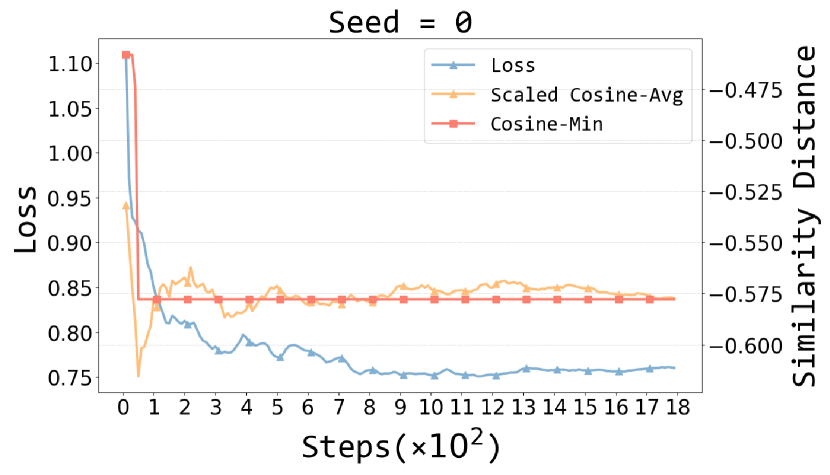
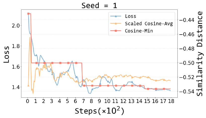
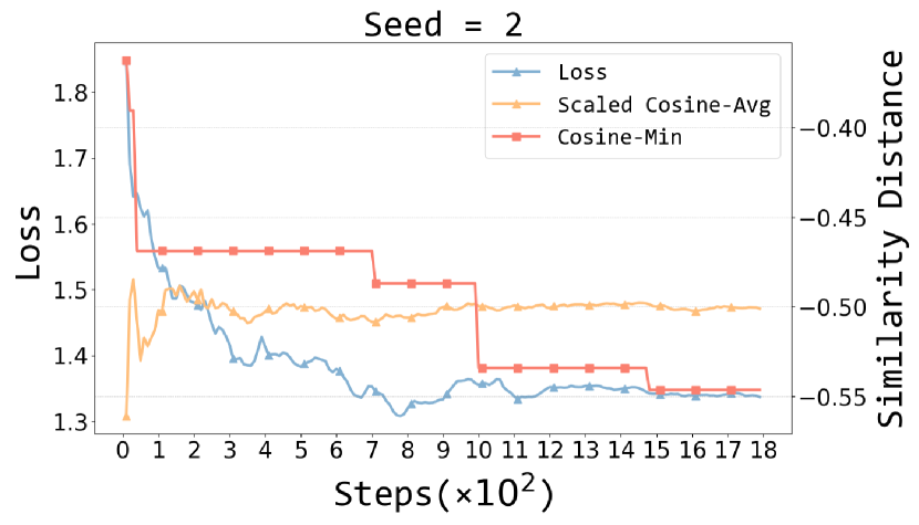
Figure 11: The loss and the similarity distances (scaled cosine average and cosine minimum) between the seen training set and the test set. Since the similarity distances calculated using the minimum (min) metric have a much larger range compared to the average (avg) metric, we consider scaling the average similarity to the same magnitude as the minimum similarity, denoted by “Scaled Cosine-Avg”. This will allow for better comparison and analysis between the two metrics.

Setting.

We analyze a series of checkpoints saved during instruction tuning on Flan-mini, based on the three settings described in Section 3.1. We calculate similarity distances between the training data seen by each checkpoint and each unseen task, as depicted in LABEL:fig:nine_similarity_with_loss. Furthermore, in the cluster setting, we explore the relationship between a significant decrease in the lowest loss observed with different seeds and the similarity measures. Specifically, suppose there are $N$ instruction-tuned checkpoints and $D$ is the similarity distance matrix, for $k^{th}$ checkpoint in the cluster setting, we compute the Scaled Cosine-Avg and Cosine-Min similarity distances as follows:

$$\text{Cosine-Min}_{k} =\text{MIN}(D[:160\times k][:])$$ (14)

$$\text{Cosine-Avg}_{k} =\text{AVG}(D[:160\times k][:])$$

$$\text{Scaled-Cosine-Avg}_{k} =\text{Cosine-Avg}_{k}\times\frac{\frac{1}{N}\sum_{k=1}^{N}\text{Cosine-Min}_{k}}{\frac{1}{N}\sum_{k=1}^{N}\text{Cosine-Avg}_{k}}$$

Results.

We found a strong correlation between the trends of similarity calculated using minimal measure and the trends of loss. In the leftmost plot of LABEL:fig:nine_similarity_with_loss, we observe sudden drops in both the cluster setting (red) and the similarity distances calculated using the minimal measure around step 450 and step 1150. Interestingly, the magnitude of these drops in similarity distances and loss appears coincidental. Furthermore, in Figure 11, we notice that for $seed=0$ (left), the Cosine-Min (red) decreases to around -0.58 at approximately 50 steps. In contrast, for $seed=1$ (middle) and $seed=2$ (right), the Cosine-Min (red) drops below -0.5 at around 700 steps and 1,000 steps, respectively. Additionally, the lowest loss for $seed=0$ (left) is significantly lower and exhibits a more stable decrease over time compared to the other two seeds.

Additionally, after carefully examining all 225 unseen tasks, among the nine similarity distance metrics, we observed that the i) fluctuation patterns are almost identical when using Euclidean and cosine distances, as well as when using centroid and average distances; ii) the sudden decrease observed in the loss curve in the preceding subsections seems to coincide with sharp drops when using the minimum distance calculation; iii) the KL divergence does not exhibit a clear pattern of change in relation to the loss, which may be due to the fact that KL divergence calculates differences based on n-gram distributions, without taking into account semantic information; iv) the “max” metric focuses on the least similar data encountered during the instruction tuning process.

For the model during instruction tuning, Cosine-Avg reflects the average distance from the seen training set to the test set, providing an overall perspective on the impact of seen samples on the test set. On the other hand, Cosine-Min reflects the impact of the closest sample in the seen training set to the test set, providing a local perspective on the influence of seen samples on the test set. Therefore, in the following experiments, we will consider using the Cosine Average (Cosine-Avg) and Cosine Minimum (Cosine-Min) embedding metrics for similarity calculation.

B.5 Proof of Optimal Substructure Property

Property of Similarity Measures.

Intuitively, we could compute the similarity distance between each training data point and the entire test set, and then reorder the training data based on this similarity distance. In this way, the model encounters the most similar training data point to the test set first during instruction tuning. We demonstrate that this approach exhibits the characteristics of optimal substructure:

Theorem B.1 (Optimal Substructure of Cosine-Avg and Cosine-Min)

Let $f$ be a function for calculating dataset-level similarity distance (Cosine-Avg and Cosine-Min), taking two sets $A$ and $B$ as inputs and outputting a real number. Given a training set $\mathcal{D}_{\text{train}}$ and a test set $\mathcal{D}_{\text{test}}$, assume $\mathcal{D}_{\text{train}}^{f}$ is obtained by reordering $\mathcal{D}_{\text{train}}$ based on the function $f$ in ascending order of similarity distance to $\mathcal{D}_{\text{test}}$. For any $i^{th}$ and $j^{th}$ training data $x_{i}$ and $x_{j}$ ($i<j$) in $\mathcal{D}_{\text{train}}^{f}$, naturally, we have $f(\{x_{i}\},\mathcal{D}_{\text{test}})\leq f(\{x_{j}\},\mathcal{D}_{\text{test}})$. We also have that,

$$f(\mathcal{D}_{\text{train}}^{f}[:i],\mathcal{D}_{\text{test}})\leq f(\mathcal{D}_{\text{train}}^{f}[:j],\mathcal{D}_{\text{test}})$$ (15)

The characteristic of optimal substructure ensures that the effect of training set permutation according to Cosine-Avg or Cosine-Min can accumulate over time as more data point is presented to the model.

Proof of Theorem B.1.

Let $f$ be a function for calculating dataset-level similarity distance (Cosine-Avg and Cosine-Min), taking two sets $A$ and $B$ as inputs and outputting a real number. Suppose the reordered training dataset $\mathcal{D}_{\text{train}}^{f}$ follows the sequence from the front to the end: {$x_{1}$, $x_{2}$, $\cdots$, $x_{i}$, $x_{i+1}$, $\cdots$, $x_{j}$, $x_{j+1}$, $\cdots$}, we consider the unary function $g(i)=f(\{x_{i}\},\mathcal{D}_{\text{test}})$, where $i\in[1,2,3,\cdots]$. Due to the reordering, the function $g(i)$ is monotonically non-decreasing. We have that:

$$f(\mathcal{D}_{\text{train}}^{f}[:i],\mathcal{D}_{\text{test}})\leq f(\mathcal{D}_{\text{train}}^{f}[:j],\mathcal{D}_{\text{test}})$$ (16)

Firstly, for Cosine-Avg, suppose the length of $\mathcal{D}_{\text{test}}$ is $N_{\text{test}}$ we have

$$f(\mathcal{D}_{\text{train}}^{f}[:i],\mathcal{D}_{\text{test}})=\frac{1}{i\times N_{\text{test}}}\sum_{p=1}^{i}\sum_{q=1}^{N_{\text{test}}}Cosine(x_{p},y_{q}),\ \ x_{p}\in\mathcal{D}_{\text{train}}^{f},y_{q}\in\mathcal{D}_{\text{test}}$$ (17)

By applying the $g(i)$ function, we have that

$$f(\mathcal{D}_{\text{train}}^{f}[:i],\mathcal{D}_{\text{test}})=\frac{1}{i}\sum_{p=1}^{i}g(p)$$ (18)

Similarly, we have

$$f(\mathcal{D}_{\text{train}}^{f}[:j],\mathcal{D}_{\text{test}})=\frac{1}{j}\sum_{p=1}^{j}g(p)$$ (19)

We notice that

$$\frac{1}{j}\sum_{p=1}^{j}g(p)-\frac{1}{i}\sum_{p=1}^{i}g(p) =\frac{i\sum_{p=1}^{j}g(p)-j\sum_{p=1}^{i}g(p)}{ij}$$ (20)

$$=\frac{i\sum_{p=i+1}^{j}g(p)-(j-i)\sum_{p=1}^{i}g(p)}{ij}$$

$$\geq\frac{i\sum_{p=i+1}^{j}g(i)-(j-i)\sum_{p=1}^{i}g(i)}{ij}$$

$$=\frac{i(j-i)g(p)-(j-i)ig(p)}{ij}$$

$$=0$$

Similarly for Cosine-Min, we have:

$$f(\mathcal{D}_{\text{train}}^{f}[:j],\mathcal{D}_{\text{test}})-f(\mathcal{D}_{\text{train}}^{f}[:j],\mathcal{D}_{\text{test}}) =\min_{1\leq p\leq j}g(p)-\min_{1\leq p\leq i}g(p)$$ (21)

$$\geq\min_{1\leq p\leq i}g(p)-\min_{1\leq p\leq i}g(p)$$

$$=0$$

The uses of $\geq$ in the expressions are due to the monotonically non-decreasing property of the $g(i)$ function. Thus, the original expression is proved.

Appendix C Details for Section 4

C.1 Data

We utilized three datasets: Flan-mini [14], ShareGPT (GPT4) [46] and NoRobots [35]. Here, we provide a detailed overview of ShareGPT (GPT4) and NoRobots.

ShareGPT

ShareGPT contains cleaned and filtered 6k expert conversations generated by GPT-4 used to train OpenChat [46]. We use the version from openchat .

NoRobots

NoRobots is a high-quality English dataset of 10K instructions and demonstrations created by skilled human annotators rather than GPTs. It was modeled after the instruction dataset described in OpenAI’s InstructGPT paper [28] and is comprised mostly of single-turn instructions.

Concatenating the various fields from the data, examples of complete training data appear as follows:

  ShareGPT example

⬇

<s>User: I want you to become my Prompt engineer. Your goal is to help me craft the best possible\n prompt for my needs. The prompt will be used by you, ChatGPT. You will follow the\n following process:\n\n1. Your first response will be to ask me what the prompt should be about. I will provide my\n answer, but we will need to improve it through continual iterations by going through the\n next steps.\n\n2. Based on my input, you will generate 2 sections. a) Revised prompt (provide your\n rewritten prompt. it should be clear, concise, and easily unders]god by you), b) Questions\n(ask any relevant questions pertaining to what additional information is needed from me to\n improve the prompt).\n\n3. We will continue this iterative process with me providing additional information to you\n and you updating the prompt in the Revised prompt section until I say we are done.

Assistant: What would you like the prompt to be about?</s>

  NoRobots example

⬇

<s>User: What is the fastest flying bird?

Assistant: The fastest-flying bird is the Peregrine Falcon. When diving, it has been measured at speeds over 186 miles per hour.</s>

C.2 Experimental Setup

Flan-mini.

We randomly selected several tasks as the testing set, while using all the data from the remaining tasks as the training set. Based on the findings in Section 2, which demonstrated that zero-shot generalization occurs early during instruction tuning, we decided to sample around 30,000 data points, maintaining a similar scale to our previous experiments to conserve resources.

ShareGPT & NoRobots.

We randomly select 200 data points as the testing set, while using all the remaining data points as the training set.

Settings.

For the three datasets mentioned above, we permute the training set based on the Test-centric Multi-turn Arrangement. Assuming that we select each turn of training data from the nearest to the farthest, denoted as $\mathcal{D}_{\text{train}}^{i}(i\in[1,N])$, where $N$ represents the total number of rounds. Similar to the experiments in Section 3, we have also configured the following three settings, while ensuring that the only difference between these three settings is the permutation of the same dataset:

• NFT (Nearest First Training): We sequentially organize the data for $\mathcal{D}_{\text{train}}^{i}$ from $i=1$ to $i=N$.

• FFT (Farthest First Training): We sequentially organize the data for $\mathcal{D}_{\text{train}}^{i}$ from $i=N$ to $i=1$.

• RT (Random Training): As a baseline, we randomly shuffle all training data.

C.3 Combining Training Data from Different Turns at a More Macroscopic Level

Settings.

In the case of Flan-mini, we randomly selected several tasks as the testing set while using all the data from the remaining tasks as the training set. Instead of randomly sampling 30k examples first, we apply the Test-centric Multi-turn Arrangement method to the whole training data, which exceeded 1 million instances. Assuming that we select each turn of training data from the nearest to the farthest, denoted as $\mathcal{D}_{\text{train}}^{i}(i\in[1,N])$, where $N$ represents the total number of rounds. We assume that $M$ represents the desired number of training data samples we want to obtain. We considered the following five settings:

• NFT (Nearest First Training): Firstly, we sequentially organize the data for $\mathcal{D}_{\text{train}}^{i}$ from $i=1$ to $i=N$ until the accumulated amount exceeds $\frac{M}{2}$, resulting in the dataset $\mathcal{D}_{\text{train1}}$. Subsequently, we proceed to sequentially organize the data for $\mathcal{D}_{\text{train}}^{i}$ from $i=N$ to $i=1$ until the accumulated amount exceeds $\frac{M}{2}$, yielding the dataset $\mathcal{D}_{\text{train2}}$. Finally, we merge $\mathcal{D}_{\text{train1}}$ and $\mathcal{D}_{\text{train2}}$ while ensuring that the data is ordered from nearest to farthest.

• FFT (Farthest First Training): We merge $\mathcal{D}_{\text{train1}}$ and $\mathcal{D}_{\text{train2}}$ in the NFT setting while ensuring that the data is ordered from farthest to nearest.

• RT (Random Training): As a baseline, we randomly shuffle all training data.

• MAX: We sequentially organize the data for $\mathcal{D}_{\text{train}}^{i}$ from $i=N$ to $i=1$ until the accumulated amount exceeded $M$.

• MIN: We sequentially organize the data for $\mathcal{D}_{\text{train}}^{i}$ from $i=1$ to $i=N$ until the accumulated amount exceeded $M$.

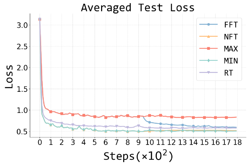
Figure 12: Averaged test loss on five similarity settings under Test-centric Multi-turn Arrangement on Flan-mini.

Results.

Early exposure to highly similar training data is beneficial for generalization while accessing high-similarity data during instruction tuning can facilitate continued learning and further loss reduction. From Figure 12, we find that i) NFT (yellow) and MIN (green) loss curves exhibited nearly identical patterns. This indicates that early exposure to training data that closely resembles the test data is advantageous for generalization. ii) On the other hand, FFT (blue) and MAX (red) loss curves diverged around the halfway point of training (at 950 steps). At this stage, FFT (blue) began encountering training data with high similarity to the test data, resulting in a further decrease in loss. This suggests that accessing high-similarity data during the instruction tuning phase can lead to improved performance. iii) RT (purple) occupied an intermediate position between the other approaches and served as a baseline. This suggests that RT, which follows a random training strategy, falls between the extremes of NFT and FFT in terms of performance.

C.4 A Deeper Understanding of Test-centric Multi-turn Arrangement

In the main text, we introduce the Test-centric Multi-turn Arrangement method, inspired by transportation theory. In transportation theory, we consider the calculation of the minimum cost required to transform a probability distribution $P(x)$ of a random variable $X$ into another probability distribution $Q(y)$ of a random variable $Y$. This minimum cost is defined as the Optimal Transport Divergence, as follows:

$$\text{OT}(P||Q)=\inf_{\gamma\in\Gamma(P,Q)}\mathbb{E}_{(x,y)\sim\gamma}[c(x,y)]$$ (22)

where $\Gamma(P,Q)$ denotes the set of all joint distributions $\gamma(x,y)$ whose marginals are $P(x)$ and $Q(y)$, respectively, and $c(x,y)$ represents the cost function measuring the "distance" between $x$ and $y$. A commonly used definition for $c(x,y)$ is the Euclidean distance between two points, which can also be understood as the square of the $L2$ norm. This leads to the definition of the 2-Wasserstein Distance:

$$W_{2}(P,Q)=\left(\inf_{\gamma\in\Gamma(P,Q)}\mathbb{E}_{(x,y)\sim\gamma}[\|x-y\|^{2}]\right)^{\frac{1}{2}}$$ (23)

More generally, the $k$-Wasserstein Distance is defined as follows:

$$W_{k}(P,Q)=\left(\inf_{\gamma\in\Gamma(P,Q)}\mathbb{E}_{(x,y)\sim\gamma}[\|x-y\|^{k}]\right)^{\frac{1}{k}}$$ (24)

This definition uses the $k$-th power of the $L2$ norm as the cost function, providing a generalized measure of the "transportation cost" between probability distributions.

In our article, we highlight the significant impact of the similarity between training data and test data on zero-shot generalization. Therefore, a natural question arises: how can we permute the training data using a better similarity distance measure to achieve better zero-shot generalization? Based on Optimal Transport Divergence, we can formalize our problem as follows:

$$\text{Minimize }\sum_{i=1}^{n}\sum_{j=1}^{m}\gamma_{ij}c(x_{i},y_{j})$$ (25)

subject to the constraints:

$$\sum_{j=1}^{m}\gamma_{ij} =P(x_{i})=\frac{1}{n}, \forall i=1,\ldots,n$$ (26)

$$\sum_{i=1}^{n}\gamma_{ij} =Q(y_{j})=\frac{1}{m}, \forall j=1,\ldots,m$$

where $\gamma_{ij}$ is the transport plan that minimizes the overall transportation cost between the distributions of the training data $P(x)$ and the test data $Q(y)$. The cost function $c(x,y)$ typically represents the Euclidean distance (L2 norm) between points $x$ and $y$.

The above method treats the distributions $P(x)$ and $Q(y)$ of training and test data as uniform, but this assumption fails when $n$ (training data) and $m$ (test data) are significantly different, causing each training data point to have much less impact compared to each test data point. Hence, we consider treating training and test data equally, with the constraint that the $\Gamma$ matrix contains only 0 or 1 elements. To bridge this gap, we propose the heuristic Test-centric Multi-turn Arrangement method in Algorithm 1 to address the imbalance between training and test data in zero-shot generalization.

This method ensures that each training data point is selected in exactly one round. For the $k$-th round of selected training data $\mathcal{D}_{\text{train}}^{k}$, for each $x_{i}$ in $\mathcal{D}_{\text{train}}^{k}$, there exists a test data point $y_{j}$ such that $c(x_{i},y_{j})$ is the $k$-th smallest element in the $j$-th column of the Cost Matrix $\mathcal{C}$ with each entry $c(x_{i},y_{j})$.

By ensuring this, we achieve a balanced selection of training data points that are optimally distributed according to their similarity to the test data, facilitating more effective zero-shot generalization.

Appendix D Limitations

Although our research has made significant progress by discovering that zero-shot generalization occurs in the early stage of instruction tuning and proposing various similarity distance measures to explore their impact on zero-shot generalization, we acknowledge that our study is far from perfect. Firstly, conducting a single experiment can be costly due to storage space requirements and computational resource limitations, so we only conducted limited explorations on a subset of datasets (NIV2, P3, flan-mini) using LLaMA-2-7B with a few runs, which may introduce biases in our conclusions. Secondly, the similarity distance measures we proposed may not have a strong theoretical foundation and can only serve as supplements to existing measures. Lastly, we chose loss as the metric for zero-shot generalization instead of traditional task-level evaluations often seen in benchmarks like MT-Bench. This is because we believe that traditional task-level generalization has certain limitations, as different tasks or categories may still appear relatively similar to LLMs, while instances from the same task may exhibit profound differences. However, this viewpoint still requires further validation. We hope future works can address these limitations.

Appendix E Compute Resources

All experiments in this study were conducted on multiple 80GB A800 instances, known for their high-performance capabilities. Conducting full-parameter instruction tuning of LLaMA-2-7B, with approximately 30,000 training data points, utilizing two 80GB A800 instances, required approximately 8 hours. The evaluation pipeline, which involved calculating loss on a series of fine-grained instruction-tuned checkpoints, was executed using a single 80GB A800 instance, taking approximately 10 hours. It is worth noting that the overall research project demanded a greater amount of compute resources than what is solely reported in this paper. This includes additional computational resources utilized for preliminary experiments and unsuccessful attempts that were not included in the final paper.

Appendix F Broader Impacts

Our work is dedicated to understanding the mechanisms of zero-shot generalization during instruction tuning and proposing several methods to enhance zero-shot generalization. This contributes to improving the generalization ability of generative models on unseen tasks. However, it is important to note that these techniques could potentially be utilized for enhancing generalization on harmful tasks as well. Therefore, ethical considerations and responsible deployment of such methods are crucial to ensure their appropriate and beneficial use. Possible mitigation strategies should be conducted, for example, clear policies should be implemented to govern their responsible use while engaging stakeholders to gather diverse perspectives.

NeurIPS Paper Checklist

1. Claims

2. Question: Do the main claims made in the abstract and introduction accurately reflect the paper’s contributions and scope?

3. Answer: [Yes]

4. Justification: See Sections 2, 3 and 4.

5. Guidelines:

   • The answer NA means that the abstract and introduction do not include the claims made in the paper.

   • The abstract and/or introduction should clearly state the claims made, including the contributions made in the paper and important assumptions and limitations. A No or NA answer to this question will not be perceived well by the reviewers.

   • The claims made should match theoretical and experimental results, and reflect how much the results can be expected to generalize to other settings.

   • It is fine to include aspirational goals as motivation as long as it is clear that these goals are not attained by the paper.

6. Limitations

7. Question: Does the paper discuss the limitations of the work performed by the authors?

8. Answer: [Yes]

9. Justification: See Appendix D.

10. Guidelines:

    • The answer NA means that the paper has no limitation while the answer No means that the paper has limitations, but those are not discussed in the paper.

    • The authors are encouraged to create a separate "Limitations" section in their paper.

    • The paper should point out any strong assumptions and how robust the results are to violations of these assumptions (e.g., independence assumptions, noiseless settings, model well-specification, asymptotic approximations only holding locally). The authors should reflect on how these assumptions might be violated in practice and what the implications would be.

    • The authors should reflect on the scope of the claims made, e.g., if the approach was only tested on a few datasets or with a few runs. In general, empirical results often depend on implicit assumptions, which should be articulated.

    • The authors should reflect on the factors that influence the performance of the approach. For example, a facial recognition algorithm may perform poorly when image resolution is low or images are taken in low lighting. Or a speech-to-text system might not be used reliably to provide closed captions for online lectures because it fails to handle technical jargon.

    • The authors should discuss the computational efficiency of the proposed algorithms and how they scale with dataset size.

    • If applicable, the authors should discuss possible limitations of their approach to address problems of privacy and fairness.

    • While the authors might fear that complete honesty about limitations might be used by reviewers as grounds for rejection, a worse outcome might be that reviewers discover limitations that aren’t acknowledged in the paper. The authors should use their best judgment and recognize that individual actions in favor of transparency play an important role in developing norms that preserve the integrity of the community. Reviewers will be specifically instructed to not penalize honesty concerning limitations.

11. Theory Assumptions and Proofs

12. Question: For each theoretical result, does the paper provide the full set of assumptions and a complete (and correct) proof?

13. Answer: [Yes]

14. Justification: See Theorem B.1 and proof in Section B.5.

15. Guidelines:

    • The answer NA means that the paper does not include theoretical results.

    • All the theorems, formulas, and proofs in the paper should be numbered and cross-referenced.

    • All assumptions should be clearly stated or referenced in the statement of any theorems.

    • The proofs can either appear in the main paper or the supplemental material, but if they appear in the supplemental material, the authors are encouraged to provide a short proof sketch to provide intuition.

    • Inversely, any informal proof provided in the core of the paper should be complemented by formal proofs provided in appendix or supplemental material.

    • Theorems and Lemmas that the proof relies upon should be properly referenced.

16. Experimental Result Reproducibility

17. Question: Does the paper fully disclose all the information needed to reproduce the main experimental results of the paper to the extent that it affects the main claims and/or conclusions of the paper (regardless of whether the code and data are provided or not)?

18. Answer: [Yes]

19. Justification: See details of main experimental setup in Appendices A, B and C, and we have also provided the code, as well as the links to the data and the model we used.

20. Guidelines:

    • The answer NA means that the paper does not include experiments.

    • If the paper includes experiments, a No answer to this question will not be perceived well by the reviewers: Making the paper reproducible is important, regardless of whether the code and data are provided or not.

    • If the contribution is a dataset and/or model, the authors should describe the steps taken to make their results reproducible or verifiable.

    • Depending on the contribution, reproducibility can be accomplished in various ways. For example, if the contribution is a novel architecture, describing the architecture fully might suffice, or if the contribution is a specific model and empirical evaluation, it may be necessary to either make it possible for others to replicate the model with the same dataset, or provide access to the model. In general. releasing code and data is often one good way to accomplish this, but reproducibility can also be provided via detailed instructions for how to replicate the results, access to a hosted model (e.g., in the case of a large language model), releasing of a model checkpoint, or other means that are appropriate to the research performed.

    • While NeurIPS does not require releasing code, the conference does require all submissions to provide some reasonable avenue for reproducibility, which may depend on the nature of the contribution. For example

      1. If the contribution is primarily a new algorithm, the paper should make it clear how to reproduce that algorithm.

      2. If the contribution is primarily a new model architecture, the paper should describe the architecture clearly and fully.

      3. If the contribution is a new model (e.g., a large language model), then there should either be a way to access this model for reproducing the results or a way to reproduce the model (e.g., with an open-source dataset or instructions for how to construct the dataset).

      4. We recognize that reproducibility may be tricky in some cases, in which case authors are welcome to describe the particular way they provide for reproducibility. In the case of closed-source models, it may be that access to the model is limited in some way (e.g., to registered users), but it should be possible for other researchers to have some path to reproducing or verifying the results.

21. Open access to data and code

22. Question: Does the paper provide open access to the data and code, with sufficient instructions to faithfully reproduce the main experimental results, as described in supplemental material?

23. Answer: [Yes]

24. Justification: We have provided the code and links to public datasets used to reproduce our results.

25. Guidelines:

    • The answer NA means that paper does not include experiments requiring code.

    • Please see the NeurIPS code and data submission guidelines (https://nips.cc/public/guides/CodeSubmissionPolicy) for more details.

    • While we encourage the release of code and data, we understand that this might not be possible, so “No” is an acceptable answer. Papers cannot be rejected simply for not including code, unless this is central to the contribution (e.g., for a new open-source benchmark).

    • The instructions should contain the exact command and environment needed to run to reproduce the results. See the NeurIPS code and data submission guidelines (https://nips.cc/public/guides/CodeSubmissionPolicy) for more details.

    • The authors should provide instructions on data access and preparation, including how to access the raw data, preprocessed data, intermediate data, and generated data, etc.

    • The authors should provide scripts to reproduce all experimental results for the new proposed method and baselines. If only a subset of experiments are reproducible, they should state which ones are omitted from the script and why.

    • At submission time, to preserve anonymity, the authors should release anonymized versions (if applicable).

    • Providing as much information as possible in supplemental material (appended to the paper) is recommended, but including URLs to data and code is permitted.

26. Experimental Setting/Details

27. Question: Does the paper specify all the training and test details (e.g., data splits, hyperparameters, how they were chosen, type of optimizer, etc.) necessary to understand the results?

28. Answer: [Yes]

29. Justification: See details of main experimental setup in Appendices A, B and C, and we have also provided the code, as well as the links to the data and the model we used.

30. Guidelines:

    • The answer NA means that the paper does not include experiments.

    • The experimental setting should be presented in the core of the paper to a level of detail that is necessary to appreciate the results and make sense of them.

    • The full details can be provided either with the code, in appendix, or as supplemental material.

31. Experiment Statistical Significance

32. Question: Does the paper report error bars suitably and correctly defined or other appropriate information about the statistical significance of the experiments?

33. Answer: [No]

34. Justification: Conducting a single experiment can be costly due to the requirements of consuming extensive storage space (for storing a large number of fine-grained full instruction tuning checkpoints) and computational resource limitations (for running many full instruction tuning on LLaMA-2-7B).

35. Guidelines:

    • The answer NA means that the paper does not include experiments.

    • The authors should answer "Yes" if the results are accompanied by error bars, confidence intervals, or statistical significance tests, at least for the experiments that support the main claims of the paper.

    • The factors of variability that the error bars are capturing should be clearly stated (for example, train/test split, initialization, random drawing of some parameter, or overall run with given experimental conditions).

    • The method for calculating the error bars should be explained (closed form formula, call to a library function, bootstrap, etc.)

    • The assumptions made should be given (e.g., Normally distributed errors).

    • It should be clear whether the error bar is the standard deviation or the standard error of the mean.

    • It is OK to report 1-sigma error bars, but one should state it. The authors should preferably report a 2-sigma error bar than state that they have a 96% CI, if the hypothesis of Normality of errors is not verified.

    • For asymmetric distributions, the authors should be careful not to show in tables or figures symmetric error bars that would yield results that are out of range (e.g. negative error rates).

    • If error bars are reported in tables or plots, The authors should explain in the text how they were calculated and reference the corresponding figures or tables in the text.

36. Experiments Compute Resources

37. Question: For each experiment, does the paper provide sufficient information on the computer resources (type of compute workers, memory, time of execution) needed to reproduce the experiments?

38. Answer: [Yes]

39. Justification: See Appendix E

40. Guidelines:

    • The answer NA means that the paper does not include experiments.

    • The paper should indicate the type of compute workers CPU or GPU, internal cluster, or cloud provider, including relevant memory and storage.

    • The paper should provide the amount of compute required for each of the individual experimental runs as well as estimate the total compute.

    • The paper should disclose whether the full research project required more compute than the experiments reported in the paper (e.g., preliminary or failed experiments that didn’t make it into the paper).

41. Code Of Ethics

42. Question: Does the research conducted in the paper conform, in every respect, with the NeurIPS Code of Ethics https://neurips.cc/public/EthicsGuidelines?

43. Answer: [Yes]

44. Justification: We ensure this by carefully examining all experimental setups.

45. Guidelines:

    • The answer NA means that the authors have not reviewed the NeurIPS Code of Ethics.

    • If the authors answer No, they should explain the special circumstances that require a deviation from the Code of Ethics.

    • The authors should make sure to preserve anonymity (e.g., if there is a special consideration due to laws or regulations in their jurisdiction).

46. Broader Impacts

47. Question: Does the paper discuss both potential positive societal impacts and negative societal impacts of the work performed?

48. Answer: [Yes]

49. Justification: See Appendix F

50. Guidelines:

    • The answer NA means that there is no societal impact of the work performed.

    • If the authors answer NA or No, they should explain why their work has no societal impact or why the paper does not address societal impact.

    • Examples of negative societal impacts include potential malicious or unintended uses (e.g., disinformation, generating fake profiles, surveillance), fairness considerations (e.g., deployment of technologies that could make decisions that unfairly impact specific groups), privacy considerations, and security considerations.

    • The conference expects that many papers will be foundational research and not tied to particular applications, let alone deployments. However, if there is a direct path to any negative applications, the authors should point it out. For example, it is legitimate to point out that an improvement in the quality of generative models could be used to generate deepfakes for disinformation. On the other hand, it is not needed to point out that a generic algorithm for optimizing neural networks could enable people to train models that generate Deepfakes faster.

    • The authors should consider possible harms that could arise when the technology is being used as intended and functioning correctly, harms that could arise when the technology is being used as intended but gives incorrect results, and harms following from (intentional or unintentional) misuse of the technology.

    • If there are negative societal impacts, the authors could also discuss possible mitigation strategies (e.g., gated release of models, providing defenses in addition to attacks, mechanisms for monitoring misuse, mechanisms to monitor how a system learns from feedback over time, improving the efficiency and accessibility of ML).

51. Safeguards

52. Question: Does the paper describe safeguards that have been put in place for responsible release of data or models that have a high risk for misuse (e.g., pretrained language models, image generators, or scraped datasets)?

53. Answer: [N/A]

54. Justification: Our research does not involve the creation of new datasets or training and releasing new models.

55. Guidelines:

    • The answer NA means that the paper poses no such risks.

    • Released models that have a high risk for misuse or dual-use should be released with necessary safeguards to allow for controlled use of the model, for example by requiring that users adhere to usage guidelines or restrictions to access the model or implementing safety filters.

    • Datasets that have been scraped from the Internet could pose safety risks. The authors should describe how they avoided releasing unsafe images.

    • We recognize that providing effective safeguards is challenging, and many papers do not require this, but we encourage authors to take this into account and make a best faith effort.

56. Licenses for existing assets

57. Question: Are the creators or original owners of assets (e.g., code, data, models), used in the paper, properly credited and are the license and terms of use explicitly mentioned and properly respected?

58. Answer: [Yes]

59. Justification: For the models and datasets used, we have provided references to the HuggingFace links or papers for proper citation.

60. Guidelines:

    • The answer NA means that the paper does not use existing assets.

    • The authors should cite the original paper that produced the code package or dataset.

    • The authors should state which version of the asset is used and, if possible, include a URL.

    • The name of the license (e.g., CC-BY 4.0) should be included for each asset.

    • For scraped data from a particular source (e.g., website), the copyright and terms of service of that source should be provided.

    • If assets are released, the license, copyright information, and terms of use in the package should be provided. For popular datasets, paperswithcode.com/datasets has curated licenses for some datasets. Their licensing guide can help determine the license of a dataset.

    • For existing datasets that are re-packaged, both the original license and the license of the derived asset (if it has changed) should be provided.

    • If this information is not available online, the authors are encouraged to reach out to the asset’s creators.

61. New Assets

62. Question: Are new assets introduced in the paper well documented and is the documentation provided alongside the assets?

63. Answer: [N/A]

64. Justification: The paper does not release new assets.

65. Guidelines:

    • The answer NA means that the paper does not release new assets.

    • Researchers should communicate the details of the dataset/code/model as part of their submissions via structured templates. This includes details about training, license, limitations, etc.

    • The paper should discuss whether and how consent was obtained from people whose asset is used.

    • At submission time, remember to anonymize your assets (if applicable). You can either create an anonymized URL or include an anonymized zip file.

66. Crowdsourcing and Research with Human Subjects

67. Question: For crowdsourcing experiments and research with human subjects, does the paper include the full text of instructions given to participants and screenshots, if applicable, as well as details about compensation (if any)?

68. Answer: [N/A]

69. Justification: The paper does not involve crowdsourcing nor research with human subjects.

70. Guidelines:

    • The answer NA means that the paper does not involve crowdsourcing nor research with human subjects.

    • Including this information in the supplemental material is fine, but if the main contribution of the paper involves human subjects, then as much detail as possible should be included in the main paper.

    • According to the NeurIPS Code of Ethics, workers involved in data collection, curation, or other labor should be paid at least the minimum wage in the country of the data collector.

71. Institutional Review Board (IRB) Approvals or Equivalent for Research with Human Subjects

72. Question: Does the paper describe potential risks incurred by study participants, whether such risks were disclosed to the subjects, and whether Institutional Review Board (IRB) approvals (or an equivalent approval/review based on the requirements of your country or institution) were obtained?

73. Answer: [N/A]

74. Justification: The paper does not involve crowdsourcing nor research with human subjects.

75. Guidelines:

    • The answer NA means that the paper does not involve crowdsourcing nor research with human subjects.

    • Depending on the country in which research is conducted, IRB approval (or equivalent) may be required for any human subjects research. If you obtained IRB approval, you should clearly state this in the paper.

    • We recognize that the procedures for this may vary significantly between institutions and locations, and we expect authors to adhere to the NeurIPS Code of Ethics and the guidelines for their institution.

    • For initial submissions, do not include any information that would break anonymity (if applicable), such as the institution conducting the review.

References

- [1] Mikhail Belkin, Daniel Hsu, Siyuan Ma, and Soumik Mandal. Reconciling modern machine-learning practice and the classical bias–variance trade-off. Proceedings of the National Academy of Sciences, 116(32):15849–15854, 2019.
- [2] Tom Brown, Benjamin Mann, Nick Ryder, Melanie Subbiah, Jared D Kaplan, Prafulla Dhariwal, Arvind Neelakantan, Pranav Shyam, Girish Sastry, Amanda Askell, et al. Language models are few-shot learners. Advances in neural information processing systems, 33:1877–1901, 2020.
- [3] Lichang Chen, Shiyang Li, Jun Yan, Hai Wang, Kalpa Gunaratna, Vikas Yadav, Zheng Tang, Vijay Srinivasan, Tianyi Zhou, Heng Huang, et al. Alpagasus: Training a better alpaca with fewer data. arXiv preprint arXiv:2307.08701, 2023.
- [4] Wei-Lin Chiang, Zhuohan Li, Zi Lin, Ying Sheng, Zhanghao Wu, Hao Zhang, Lianmin Zheng, Siyuan Zhuang, Yonghao Zhuang, Joseph E. Gonzalez, Ion Stoica, and Eric P. Xing. Vicuna: An open-source chatbot impressing gpt-4 with 90%* chatgpt quality, March 2023.
- [5] Hyung Won Chung, Le Hou, Shayne Longpre, Barret Zoph, Yi Tay, William Fedus, Yunxuan Li, Xuezhi Wang, Mostafa Dehghani, Siddhartha Brahma, et al. Scaling instruction-finetuned language models. Journal of Machine Learning Research, 25(70):1–53, 2024.
- [6] Aidan Clark, Diego de Las Casas, Aurelia Guy, Arthur Mensch, Michela Paganini, Jordan Hoffmann, Bogdan Damoc, Blake Hechtman, Trevor Cai, Sebastian Borgeaud, et al. Unified scaling laws for routed language models. In International conference on machine learning, pages 4057–4086. PMLR, 2022.
- [7] Ganqu Cui, Lifan Yuan, Ning Ding, Guanming Yao, Wei Zhu, Yuan Ni, Guotong Xie, Zhiyuan Liu, and Maosong Sun. Ultrafeedback: Boosting language models with high-quality feedback. arXiv preprint arXiv:2310.01377, 2023.
- [8] Ganqu Cui, Lifan Yuan, Bingxiang He, Yangyi Chen, Zhiyuan Liu, and Maosong Sun. A unified evaluation of textual backdoor learning: Frameworks and benchmarks. Advances in Neural Information Processing Systems, 35:5009–5023, 2022.
- [9] Xiang Dai, Sarvnaz Karimi, Ben Hachey, and Cecile Paris. Using similarity measures to select pretraining data for ner. arXiv preprint arXiv:1904.00585, 2019.
- [10] Xander Davies, Lauro Langosco, and David Krueger. Unifying grokking and double descent. arXiv preprint arXiv:2303.06173, 2023.
- [11] Ning Ding, Yulin Chen, Bokai Xu, Yujia Qin, Zhi Zheng, Shengding Hu, Zhiyuan Liu, Maosong Sun, and Bowen Zhou. Enhancing chat language models by scaling high-quality instructional conversations. arXiv preprint arXiv:2305.14233, 2023.
- [12] Zhengxiao Du, Aohan Zeng, Yuxiao Dong, and Jie Tang. Understanding emergent abilities of language models from the loss perspective. arXiv preprint arXiv:2403.15796, 2024.
- [13] Kavita Ganesan. Rouge 2.0: Updated and improved measures for evaluation of summarization tasks. arXiv preprint arXiv:1803.01937, 2018.
- [14] Deepanway Ghosal, Yew Ken Chia, Navonil Majumder, and Soujanya Poria. Flacuna: Unleashing the problem solving power of vicuna using flan fine-tuning. arXiv preprint arXiv:2307.02053, 2023.
- [15] Max Grusky. Rogue scores. In Proceedings of the 61st Annual Meeting of the Association for Computational Linguistics (Volume 1: Long Papers), pages 1914–1934, 2023.
- [16] Arnav Gudibande, Eric Wallace, Charlie Snell, Xinyang Geng, Hao Liu, Pieter Abbeel, Sergey Levine, and Dawn Song. The false promise of imitating proprietary llms. arXiv preprint arXiv:2305.15717, 2023.
- [17] Tom Henighan, Jared Kaplan, Mor Katz, Mark Chen, Christopher Hesse, Jacob Jackson, Heewoo Jun, Tom B Brown, Prafulla Dhariwal, Scott Gray, et al. Scaling laws for autoregressive generative modeling. arXiv preprint arXiv:2010.14701, 2020.
- [18] Shengding Hu, Xin Liu, Xu Han, Xinrong Zhang, Chaoqun He, Weilin Zhao, Yankai Lin, Ning Ding, Zebin Ou, Guoyang Zeng, et al. Predicting emergent abilities with infinite resolution evaluation. arXiv e-prints, pages arXiv–2310, 2023.
- [19] Srinivasan Iyer, Xi Victoria Lin, Ramakanth Pasunuru, Todor Mihaylov, Daniel Simig, Ping Yu, Kurt Shuster, Tianlu Wang, Qing Liu, Punit Singh Koura, et al. Opt-iml: Scaling language model instruction meta learning through the lens of generalization. arXiv preprint arXiv:2212.12017, 2022.
- [20] Jared Kaplan, Sam McCandlish, Tom Henighan, Tom B Brown, Benjamin Chess, Rewon Child, Scott Gray, Alec Radford, Jeffrey Wu, and Dario Amodei. Scaling laws for neural language models. arXiv preprint arXiv:2001.08361, 2020.
- [21] Joongwon Kim, Akari Asai, Gabriel Ilharco, and Hannaneh Hajishirzi. Taskweb: Selecting better source tasks for multi-task nlp. arXiv preprint arXiv:2305.13256, 2023.
- [22] Changho Lee, Janghoon Han, Seonghyeon Ye, Stanley Jungkyu Choi, Honglak Lee, and Kyunghoon Bae. Instruction matters, a simple yet effective task selection approach in instruction tuning for specific tasks. arXiv preprint arXiv:2404.16418, 2024.
- [23] Ziming Liu, Eric J Michaud, and Max Tegmark. Omnigrok: Grokking beyond algorithmic data. In The Eleventh International Conference on Learning Representations, 2022.
- [24] Shayne Longpre, Le Hou, Tu Vu, Albert Webson, Hyung Won Chung, Yi Tay, Denny Zhou, Quoc V Le, Barret Zoph, Jason Wei, et al. The flan collection: Designing data and methods for effective instruction tuning. In International Conference on Machine Learning, pages 22631–22648. PMLR, 2023.
- [25] modelcenter. modelcenter. https://github.com/OpenBMB/ModelCenter, 2023.
- [26] Niklas Muennighoff, Thomas Wang, Lintang Sutawika, Adam Roberts, Stella Biderman, Teven Le Scao, M Saiful Bari, Sheng Shen, Zheng-Xin Yong, Hailey Schoelkopf, et al. Crosslingual generalization through multitask finetuning. arXiv preprint arXiv:2211.01786, 2022.
- [27] Preetum Nakkiran, Gal Kaplun, Yamini Bansal, Tristan Yang, Boaz Barak, and Ilya Sutskever. Deep double descent: Where bigger models and more data hurt. Journal of Statistical Mechanics: Theory and Experiment, 2021(12):124003, 2021.
- [28] Long Ouyang, Jeffrey Wu, Xu Jiang, Diogo Almeida, Carroll Wainwright, Pamela Mishkin, Chong Zhang, Sandhini Agarwal, Katarina Slama, Alex Ray, et al. Training language models to follow instructions with human feedback. Advances in neural information processing systems, 35:27730–27744, 2022.
- [29] Alethea Power, Yuri Burda, Harri Edwards, Igor Babuschkin, and Vedant Misra. Grokking: Generalization beyond overfitting on small algorithmic datasets. arXiv preprint arXiv:2201.02177, 2022.
- [30] Cheng Qian, Chi Han, Yi Fung, Yujia Qin, Zhiyuan Liu, and Heng Ji. Creator: Tool creation for disentangling abstract and concrete reasoning of large language models. In Findings of the Association for Computational Linguistics: EMNLP 2023, pages 6922–6939, 2023.
- [31] Cheng Qian, Bingxiang He, Zhong Zhuang, Jia Deng, Yujia Qin, Xin Cong, Yankai Lin, Zhong Zhang, Zhiyuan Liu, and Maosong Sun. Tell me more! towards implicit user intention understanding of language model driven agents. arXiv preprint arXiv:2402.09205, 2024.
- [32] Cheng Qian, Shihao Liang, Yujia Qin, Yining Ye, Xin Cong, Yankai Lin, Yesai Wu, Zhiyuan Liu, and Maosong Sun. Investigate-consolidate-exploit: A general strategy for inter-task agent self-evolution. arXiv preprint arXiv:2401.13996, 2024.
- [33] Cheng Qian, Chenyan Xiong, Zhenghao Liu, and Zhiyuan Liu. Toolink: Linking toolkit creation and using through chain-of-solving on open-source model. arXiv preprint arXiv:2310.05155, 2023.
- [34] Yujia Qin, Shengding Hu, Yankai Lin, Weize Chen, Ning Ding, Ganqu Cui, Zheni Zeng, Yufei Huang, Chaojun Xiao, Chi Han, et al. Tool learning with foundation models. arXiv preprint arXiv:2304.08354, 2023.
- [35] Nazneen Rajani, Lewis Tunstall, Edward Beeching, Nathan Lambert, Alexander M. Rush, and Thomas Wolf. No robots. https://huggingface.co/datasets/HuggingFaceH4/no_robots, 2023.
- [36] Nils Reimers and Iryna Gurevych. Sentence-bert: Sentence embeddings using siamese bert-networks. arXiv preprint arXiv:1908.10084, 2019.
- [37] Victor Sanh, Albert Webson, Colin Raffel, Stephen H Bach, Lintang Sutawika, Zaid Alyafeai, Antoine Chaffin, Arnaud Stiegler, Teven Le Scao, Arun Raja, et al. Multitask prompted training enables zero-shot task generalization. arXiv preprint arXiv:2110.08207, 2021.
- [38] Rylan Schaeffer, Brando Miranda, and Sanmi Koyejo. Are emergent abilities of large language models a mirage? Advances in Neural Information Processing Systems, 36, 2024.
- [39] Prasann Singhal, Nathan Lambert, Scott Niekum, Tanya Goyal, and Greg Durrett. D2PO: Discriminator-Guided DPO with Response Evaluation Models. arXiv e-prints, page arXiv:2405.01511, May 2024.
- [40] Jie Song, Yixin Chen, Xinchao Wang, Chengchao Shen, and Mingli Song. Deep model transferability from attribution maps. Advances in Neural Information Processing Systems, 32, 2019.
- [41] Rohan Taori, Ishaan Gulrajani, Tianyi Zhang, Yann Dubois, Xuechen Li, Carlos Guestrin, Percy Liang, and Tatsunori B. Hashimoto. Stanford alpaca: An instruction-following llama model. https://github.com/tatsu-lab/stanford_alpaca, 2023.
- [42] Vimal Thilak, Etai Littwin, Shuangfei Zhai, Omid Saremi, Roni Paiss, and Joshua Susskind. The slingshot mechanism: An empirical study of adaptive optimizers and the grokking phenomenon. arXiv preprint arXiv:2206.04817, 2022.
- [43] Hugo Touvron, Louis Martin, Kevin Stone, Peter Albert, Amjad Almahairi, Yasmine Babaei, Nikolay Bashlykov, Soumya Batra, Prajjwal Bhargava, Shruti Bhosale, et al. Llama 2: Open foundation and fine-tuned chat models. arXiv preprint arXiv:2307.09288, 2023.
- [44] Vikrant Varma, Rohin Shah, Zachary Kenton, János Kramár, and Ramana Kumar. Explaining grokking through circuit efficiency. arXiv preprint arXiv:2309.02390, 2023.
- [45] Tu Vu, Tong Wang, Tsendsuren Munkhdalai, Alessandro Sordoni, Adam Trischler, Andrew Mattarella-Micke, Subhransu Maji, and Mohit Iyyer. Exploring and predicting transferability across nlp tasks. arXiv preprint arXiv:2005.00770, 2020.
- [46] Guan Wang, Sijie Cheng, Xianyuan Zhan, Xiangang Li, Sen Song, and Yang Liu. Openchat: Advancing open-source language models with mixed-quality data. arXiv preprint arXiv:2309.11235, 2023.
- [47] Yizhong Wang, Swaroop Mishra, Pegah Alipoormolabashi, Yeganeh Kordi, Amirreza Mirzaei, Atharva Naik, Arjun Ashok, Arut Selvan Dhanasekaran, Anjana Arunkumar, David Stap, Eshaan Pathak, Giannis Karamanolakis, Haizhi Lai, Ishan Purohit, Ishani Mondal, Jacob Anderson, Kirby Kuznia, Krima Doshi, Kuntal Kumar Pal, Maitreya Patel, Mehrad Moradshahi, Mihir Parmar, Mirali Purohit, Neeraj Varshney, Phani Rohitha Kaza, Pulkit Verma, Ravsehaj Singh Puri, Rushang Karia, Savan Doshi, Shailaja Keyur Sampat, Siddhartha Mishra, Sujan Reddy A, Sumanta Patro, Tanay Dixit, and Xudong Shen. Super-NaturalInstructions: Generalization via declarative instructions on 1600+ NLP tasks. In Yoav Goldberg, Zornitsa Kozareva, and Yue Zhang, editors, Proceedings of the 2022 Conference on Empirical Methods in Natural Language Processing, pages 5085–5109, Abu Dhabi, United Arab Emirates, December 2022. Association for Computational Linguistics.
- [48] Jason Wei, Maarten Bosma, Vincent Y Zhao, Kelvin Guu, Adams Wei Yu, Brian Lester, Nan Du, Andrew M Dai, and Quoc V Le. Finetuned language models are zero-shot learners. arXiv preprint arXiv:2109.01652, 2021.
- [49] Jason Wei, Yi Tay, Rishi Bommasani, Colin Raffel, Barret Zoph, Sebastian Borgeaud, Dani Yogatama, Maarten Bosma, Denny Zhou, Donald Metzler, et al. Emergent abilities of large language models. arXiv preprint arXiv:2206.07682, 2022.
- [50] Gregory Yauney, Emily Reif, and David Mimno. Data similarity is not enough to explain language model performance. arXiv preprint arXiv:2311.09006, 2023.
- [51] Lifan Yuan, Ganqu Cui, Hanbin Wang, Ning Ding, Xingyao Wang, Jia Deng, Boji Shan, Huimin Chen, Ruobing Xie, Yankai Lin, et al. Advancing llm reasoning generalists with preference trees. arXiv preprint arXiv:2404.02078, 2024.
- [52] Amir R Zamir, Alexander Sax, William Shen, Leonidas J Guibas, Jitendra Malik, and Silvio Savarese. Taskonomy: Disentangling task transfer learning. In Proceedings of the IEEE conference on computer vision and pattern recognition, pages 3712–3722, 2018.
- [53] Hao Zhao, Maksym Andriushchenko, Francesco Croce, and Nicolas Flammarion. Long is more for alignment: A simple but tough-to-beat baseline for instruction fine-tuning. arXiv preprint arXiv:2402.04833, 2024.
- [54] Wenting Zhao, Xiang Ren, Jack Hessel, Claire Cardie, Yejin Choi, and Yuntian Deng. Wildchat: 1m chatgpt interaction logs in the wild. arXiv preprint arXiv:2405.01470, 2024.
- [55] Chunting Zhou, Pengfei Liu, Puxin Xu, Srinivasan Iyer, Jiao Sun, Yuning Mao, Xuezhe Ma, Avia Efrat, Ping Yu, Lili Yu, et al. Lima: Less is more for alignment. Advances in Neural Information Processing Systems, 36, 2024.
- [56] Jing Zhou, Zongyu Lin, Yanan Zheng, Jian Li, and Zhilin Yang. Not all tasks are born equal: Understanding zero-shot generalization. In The Eleventh International Conference on Learning Representations, 2022.
- [57] Biru Zhu, Lifan Yuan, Ganqu Cui, Yangyi Chen, Chong Fu, Bingxiang He, Yangdong Deng, Zhiyuan Liu, Maosong Sun, and Ming Gu. Beat llms at their own game: Zero-shot llm-generated text detection via querying chatgpt. In Proceedings of the 2023 Conference on Empirical Methods in Natural Language Processing, pages 7470–7483, 2023.