Scalable Expressiveness through Preprocessed Graph Perturbations

Abstract.

Graph Neural Networks (GNNs) have emerged as the predominant method for analyzing graph-structured data. However, canonical GNNs have limited expressive power and generalization capability, thus triggering the development of more expressive yet computationally intensive methods. One such approach is to create a series of perturbed versions of input graphs and then repeatedly conduct multiple message-passing operations on all variations during training. Despite their expressive power, this approach does not scale well on larger graphs. To address this scalability issue, we introduce Scalable Expressiveness through Preprocessed Graph Perturbation (SE2P). This model offers a flexible, configurable balance between scalability and generalizability with four distinct configuration classes. At one extreme, the configuration prioritizes scalability through minimal learnable feature extraction and extensive preprocessing; at the other extreme, it enhances generalizability with more learnable feature extractions, though this increases scalability costs. We conduct extensive experiments on real-world datasets to evaluate the generalizability and scalability of SE2P variants compared to various state-of-the-art benchmarks. Our results indicate that, depending on the chosen SE2P configuration, the model can enhance generalizability compared to benchmarks while achieving significant speed improvements of up to 8-fold.

1. Introduction

Graph Neural Networks (GNNs) possess exceptional predictive capabilities on relational data (e.g., social networks, protein-protein interaction networks, etc.). Their applicability spans various domains, such as recommender systems (Wu et al., 2022), protein structure modeling (Gao et al., 2020), educational systems (Namanloo et al., 2022), and knowledge graph completion (Arora, 2020). However, relational data’s complexity, scale, and dynamic nature pose substantial challenges to GNNs, emphasizing the importance of improving their generalization and computational efficiency.

Message-passing GNNs (MPNNs), a popular class of GNNs, facilitate the exchange of messages between nodes to integrate their local structural and feature information within a graph. Stacking multiple layers of message-passing allows the messages to be transmitted across longer distances in the graph, thus learning more global structural information. However, this approach increases computational complexity, particularly for larger graphs, and its generalization capabilities are limited by the $1$-dimensional Weisfeiler-Lehman ($1$-WL) graph-isomorphism test (Leman and Weisfeiler, 1968).

Several approaches have been proposed to enhance the computational efficiency of message-passing GNNs. Simplified graph neural networks (SGNNs) simplifies graph neural networks by removing their non-linearities between intermediate GNN layers, thus facilitating the preprocessing of message-passing for faster training (Wu et al., 2019; Frasca et al., 2020; Louis et al., 2023; Zhang et al., 2022; Feng et al., 2020). Another acceleration approach involves sampling methods, where node neighborhoods are sampled during preprocessing (Chiang et al., 2019; Zeng et al., 2019; Shi et al., 2023; Louis et al., 2022) or message-passing (Hamilton et al., 2017; Chen et al., 2018; Huang et al., 2018; Zou et al., 2019; Ying et al., 2018a; Chen and Zhu, 2018) to reduce the number of messages during training or inference. The $1$-WL expressivity constraint also extends to these scalability approaches for message-passing GNNs.

To go beyond $1$-WL expressive power, many attempts are made. Higher-order GNNs, similar to the hierarchy in $k$-WL tests (Li et al., 2019; Maron et al., 2019), expand message-passing from individual nodes to node tuples, yielding richer representations. As an alternative approach, Feature-augmented GNNs integrate additional features like structural encodings (Bouritsas et al., 2022; Barceló et al., 2021), geodesic distances (Li et al., 2020; Zhang et al., 2021; Velingker et al., 2022), resistance distances (Velingker et al., 2022), and positional encodings (Dwivedi et al., 2022) for nodes or edges. Other approaches known as Subgraph GNNs focus on extracting multiple subgraphs for each node, using techniques such as node/edge labeling (You et al., 2021; Papp and Wattenhofer, 2022; Huang et al., 2022) or node/edge deletion (Papp et al., 2021; Huang et al., 2022; Bevilacqua et al., 2021; Rong et al., 2020). These techniques generate a variety of subgraph perturbations, enriching the graph’s representational diversity.

Despite their improved expressiveness, these approaches are less computationally efficient than the conventional GNNs. Higher-order GNNs require (at least) cubic computational complexity for message passing (Zhang and Li, 2021; Zhang and Yao, 2022). Feature-augmented GNNs can struggle with scalability, as computing augmented features (e.g., structural encodings, resistance distance, shortest path distance, etc.) is computationally expensive for large graphs. Subgraph GNNs typically involve extracting or creating multiple large subgraphs from a larger graph and processing these with GNNs. Due to potential overlap among these subgraphs, their cumulative size can significantly expand, sometimes to hundreds of times the size of the original graph, rendering them impractical for large-scale graphs. For instance, DropGNN (Papp et al., 2021) generates multiple perturbations of the graph through random node removal and applies GNN on the perturbed graphs during training to enhance expressivity. However, scalability becomes a critical concern as the number of perturbations grows, confining the method’s applicability to smaller datasets. Our approach. In our pursuit of formulating a flexible, scalable, and expressive model, we introduce Scalable Expressiveness through Preprocessed Graph Perturbation (SE2P). Our approach offers four configuration classes, each offering a unique balance between scalability and generalizability. SE2P first creates multiple perturbations of the input graph through a perturbation policy (e.g., random node removal) and then diffuses nodal features through each perturbed graph. Unlike conventional message-passing GNNs, but similar to SGNNs (Wu et al., 2019; Frasca et al., 2020; Louis et al., 2023; Zhang et al., 2022; Feng et al., 2020), the feature diffusion occurs once during preprocessing. Our SE2P differentiates from SGNNs by leveraging the expressive power offered by multiple perturbed graphs (Papp et al., 2021; Bevilacqua et al., 2021). The diffusions from each perturbation are combined, and nodal representations of all perturbations are merged to construct the final nodal profiles. Then, these profiles are subjected to a pooling operation for graph classification tasks to produce a vector representation of the entire input graph. A critical computational strength of our framework is its flexibility, allowing for the selection of aggregation functions (learnable or non-learnable), thus enabling scalable or expressive variations of many models. Depending on the selected configuration, our empirical results demonstrate significant speedup (up to $8\times$) compared to baselines while also improving the generalizability of expressive models such as DropGNN. Our experiments confirm that SE2P surpasses the generalization limitation of SGNNs (e.g., SGCNs, and SIGN) while offering comparable scalability. SE2P demonstrates flexibility in balancing expressiveness and scalability: The SE2P’s instance SE2P-C2 achieves $3$-$6\times$ speed up with comparable generalizability to baselines, while another instance SE2P-C3 maintains baseline computational requirements and enhanced generalizability by up to $1.5\%$.

2. Related Work

We review existing methods that enhance the scalability (i.e., computational efficiency) or expressiveness of Graph Neural Networks. We have identified key subdomains within these areas. Simplification Methods (Scalability). To reduce the computational burden associated with multiple message-passing layers, one strategy (Wu et al., 2019; Frasca et al., 2020; Louis et al., 2023; Feng et al., 2020; Zhang et al., 2022) is to simplify GNN architectures by removing intermediate non-linearities, thus enabling feature propagation preprocessing across the graph. Simplified Graph Convolutional Networks (SGCN) (Wu et al., 2019) introduces a diffusion matrix by removing non-linearities from multi-layer Graph Convolutional Networks (Kipf and Welling, 2016). SIGN (Frasca et al., 2020), GRAND (Feng et al., 2020), and NAFS (Zhang et al., 2022) extend SGCN to multiple diffusion matrices instead of a single one. Similarly, S3GRL (Louis et al., 2023) extends this technique to enrich the subgraph representations. However, many diffusion approaches (e.g., SGCN, SIGN, etc.) exhibit limited expressivity. Our SE2P framework leverages this feature diffusion approach while enhancing these models with graph perturbations to overcome their expressivity limitations. Sampling Methods (Scalability). The sampling techniques are deployed to control the exponential growth of receptive fields across GNN layers for better scalability. Node-based sampling methods (Hamilton et al., 2017; Ying et al., 2018a; Chen and Zhu, 2018) samples fixed-size nodes’ neighborhoods for message-passing within mini-batches to reduce the nodes involved in the message-passing process. In contrast, layer-based sampling methods (Chen et al., 2018; Huang et al., 2018; Zou et al., 2019) targets the architectural level of GNNs by selectively sampling nodes for each layer. Subgraph-based sampling (Chiang et al., 2019; Zeng et al., 2019; Shi et al., 2023; Louis et al., 2022) focuses on sampling subgraphs during preprocessing to handle large graphs on limited memory, and integrates these smaller, representative subgraphs into minibatches during training to update embeddings. Despite scalability, these sampling methods are limited to the $1$-WL isomorphism test, necessitating enhancements in GNN expressivity.

Higher-order GNNs (Expressivity). Inspired by the higher-order WL tests (Morris et al., 2017), higher-order GNNs pass messages between node tuples instead of individual nodes (Morris et al., 2019; Azizian and Lelarge, 2020). To offset their high computational demands, localized and sparse higher-order aggregation methods have been developed (Morris et al., 2020b), with the cost of reduced expressiveness (Morris et al., 2022).

Subgraph GNNs or Perturbed GNNs (Expressivity). An emerging body of research has focused on generating a bag of subgraphs (or perturbations) from an input graph and then applying GNNs on all subgraphs to get more expressive nodal representations. The primary distinction between these approaches is how subgraphs are generated or sampled. Some common techniques include node dropping (Papp et al., 2021; Cotta et al., 2021; Feng et al., 2020), edge dropping (Bevilacqua et al., 2021; Rong et al., 2020), node marking (Papp and Wattenhofer, 2022), and ego-networks (Zhao et al., 2022; Zhang and Li, 2021; You et al., 2021). The methods involving the removal of nodes or edges can also be viewed as regularization tools for GNNs, helping to reduce over-fitting (Feng et al., 2020; Rong et al., 2020). However, these methods often require a large number of perturbed graphs (or subgraphs) for each input graph, proportional to the graph size. For example, the number of perturbations that DropGNN (Papp et al., 2021) requires is set to be the average node degree (e.g., 75 perturbed graphs for each graph in the COLLAB dataset). Applying GNNs to this many perturbed graphs for a single input graph proves to be impractical, hindering scalability. Our approach shares some similarities with this body of research in generating perturbed graphs, albeit with a notable distinction: By once preprocessing diffused features of perturbed graphs, we ease the training computations, thus significantly improving scalability compared to DropGNN and other similar methods. Feature augmented GNNs (Expressivity). Several studies have aimed to increase the expressiveness of GNNs by enriching or augmenting node features. Some examples of auxiliary/augmented node information include geodesic distances (Li et al., 2020; Zhang et al., 2021; Velingker et al., 2022), resistance distances (Velingker et al., 2022), subgraph-induced structural information (Bouritsas et al., 2022; Barceló et al., 2021), and positional encodings (Dwivedi et al., 2022). Despite the potential of feature augmentation to improve expressiveness, they fall short in scalability, as computation of the auxiliary features (e.g., substructure counts, the shortest distance between pairs, etc.) is expensive for large graphs.

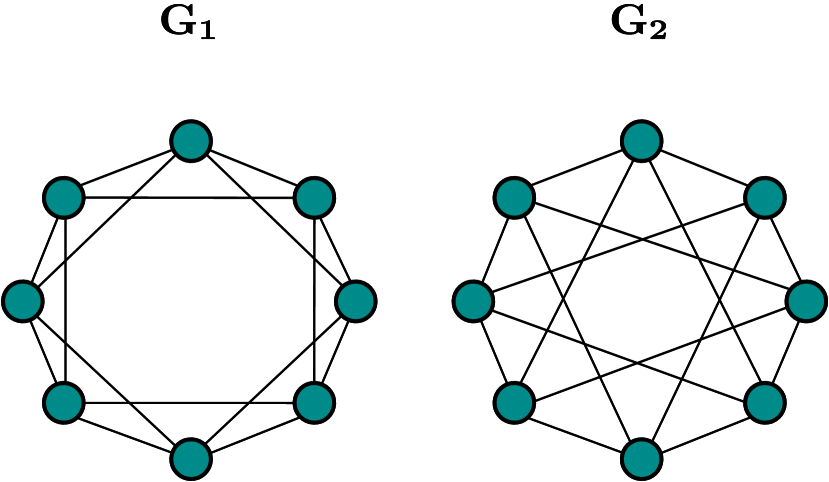
((a)) Two non-isomorphic graphs, indistinguishable by 1-WL test with the same label distributions.

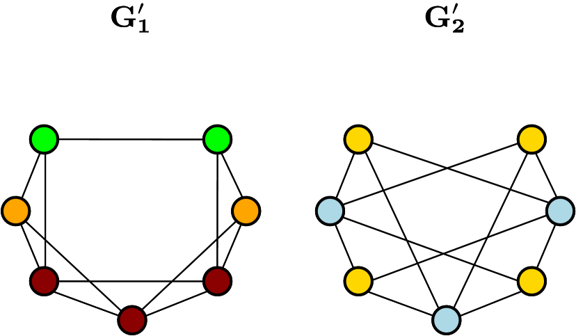
((b)) Perturbed input graphs, distinguishable by 1-WL test with different label distributions.

Figure 1. $1$-WL graph isomorphism test (a) fails to distinguish between two non-isomorphic graphs $G_{1}$ and $G_{2}$, but (b) successfully detect their perturbation (through node removal) $G_{1}^{\prime}$ and $G_{2}^{\prime}$.

3. Preliminary and Background

We consider an undirected graph $G=(V,E)$ with $|V|=n$ nodes, $|E|=m$ edges, and adjacency matrix $\mathbf{A}\in\mathbb{R}^{{n}\times{n}}$. Each node $i\in V$ possesses the $d$-dimensional feature vector $\mathbf{x}_{i}\in\mathbb{R}^{n}$, which can be viewed as the $i$-th row of $n\times d$ feature matrix $\mathbf{X}$.

3.1. Graph Prediction Task

Graph classification or regression involves predicting a label (e.g., carcinogenicity classification (Toivonen et al., 2003)) or a property (e.g., molecule solubility level (Gilmer et al., 2017)) for an entire graph based on its structure and associated features (e.g., node or edge features). Specifically, the task is formulated as a supervised learning problem, aiming to learn a mapping function $f:\mathcal{G}\to\mathcal{Y}$, given a labeled dataset $D=\{(G_{i},y_{i})\}$, where $\mathcal{G}$ is input space, and $\mathcal{Y}$ is class label space (or real for regression), $G_{i}$ is input graph sample, and $y_{i}$ is an expected label (or property). Graph Neural Networks have demonstrated significant success in effectively addressing the challenges of graph classification or regression tasks (Hamilton, 2020).

3.2. Graph Neural Networks

In message-passing Graph Neural Networks (GNNs), each node’s representation $\mathbf{h}_{i}$ is iteratively updated and refined through the aggregation of messages received from its neighbor’s representations. In GNNs, the node $i$’s representation at step (or layer) $l$ is updated by:

(1) $$\mathbf{h}_{i}^{(l)}=\operatorname{UPDATE}\left(\mathbf{h}_{i}^{(l-1)},\mathbf{m}_{N(i)}^{(l-1)}\right)$$

where $\mathbf{m}_{N(i)}^{(l-1)}$ is the message aggregated from $i$’s neighborhood $N(i)$:

(2) $$\mathbf{m}_{N(i)}^{(l-1)}=\operatorname{AGGREGATE}\left(\left\{\mathbf{h}_{j}^{(l-1)}\middle|j\in N(i)\right\}\right).$$

GNNs usually differ from one another in how their $\operatorname{AGGREGATE}$ and $\operatorname{UPDATE}$ functions are defined. For example, graph convolutional networks (GCN) (Kipf and Welling, 2016) employ a degree-normalized weighted mean as the $\operatorname{AGGREGATE}$ function:

(3) $$\mathbf{m}_{N(i)}^{(l-1)}=\sum_{j\in N(i)}\frac{\mathbf{h}_{j}^{(l-1)}}{\sqrt{|N(i)||N(j)|}},$$

followed by a simple update function of:

(4) $$\mathbf{h}_{i}^{(l)}=\sigma\left(\mathbf{W}^{(l)}\left(\frac{\mathbf{h}_{i}^{(l-1)}}{|N(i)|}+{\mathbf{m}}_{N(i)}^{(l-1)}\right)\right),$$

where $\sigma$ is a non-linearity function (e.g., ReLU), and $\mathbf{W}^{(l)}$ is the $l^{th}$ layer’s learnable weight matrix. In GNNs, for each node $i\in V$, the initial node representation at step $0$ is usually set to their original node features: $\mathbf{h}_{i}^{(0)}=\mathbf{x}_{i}$. After $L$ message-passing iterations, the node $i$’s representation $\mathbf{z}_{i}$ is the output of layer $L$, i.e., $\mathbf{z}_{i}=\mathbf{h}_{i}^{(L)}$, or a combination of all $L$ layers’ outputs $\mathbf{z}_{i}=\operatorname{COMBINE}(\mathbf{h}_{i}^{(1)},\dots,\mathbf{h}_{i}^{(L)})$ (Xu et al., 2018). One can view all learned node’s representations in the form $n\times d^{\prime}$ matrix $\mathbf{Z}$, where $d^{\prime}$ is the hidden dimensionality. All nodes’ final representations are then aggregated to form a graph (vector) representation:

(5) $$\mathbf{z}_{G}=\operatorname{POOL}\left(\left\{\mathbf{z}_{i}\middle|i\in G\right\}\right),$$

where the $\operatorname{POOL}$ function can be non-adaptive (e.g., element-wise mean or max) or adaptive (e.g., top-k pooling (Lee et al., 2019a; Gao and Ji, 2019), set transformer (Buterez et al., 2022), or MLP (Buterez et al., 2022)). The class probabilities are then computed by passing $\mathbf{z}_{G}$ through a non-linear learnable transformation (e.g., MLP).

Despite the success of GNNs, their expressive power is limited and upper bounded by the $1$-WL test (Xu et al., 2019; Morris et al., 2019). This limitation necessitates the development of new approaches with enhanced expressiveness.

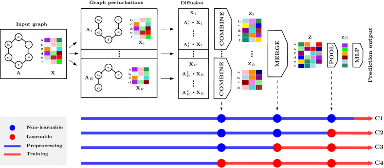
Figure 2. The SE2P framework first generates $R$ perturbations of the input graph, where each perturbation involves randomly removing some nodes, thereby resulting in new adjacency and feature matrices ${(\mathbf{A}_{r},\mathbf{X}_{r})}$. Next, node features are diffused for each perturbation by a set of diffusion matrices: the perturbed adjacency matrix powers. Then, the $\operatorname{COMBINE}$ function combines these diffused features for each perturbed graph to produce feature matrices $\mathbf{Z}_{r}$. All these matrices then undergo the $\operatorname{MERGE}$ function to generate a single nodal representation matrix $\mathbf{Z}$ for the input graph. Focusing on the graph-level task, we then apply $\operatorname{POOL}$ to yield a graph (vector) representation $z_{G}$ and further achieve the predicted output through a non-linear transformation by MLP. The functions $\operatorname{COMBINE}$, $\operatorname{MERGE}$, and $\operatorname{POOL}$ can be either non-learnable (blue circle) or learnable (red circle). This flexibility allows us to choose between different configuration classes (C1, C2, C3, and C4) to balance scalability, achieved by including more preprocessing steps (blue line), and expressivity, achieved by having more learnable components and a longer training phase (red line).

3.3. Perturbed Graph Neural Networks

To overcome $1$-WL expressivity limitation of canonical GNNs (Xu et al., 2019; Morris et al., 2019), Perturbed GNNs (e.g., DropGNN (Papp et al., 2021)) applies a shared GNN on $R$ different perturbations of the input graph (during both training and testing). For each perturbation $(\mathbf{A}_{r},\mathbf{X}_{r})$, some graph structure (e.g., nodes or edges) is randomly changed. For example, DropGNN randomly drops out some nodes for each perturbation, allowing a shared $L$-layer GNN to operate on a slightly perturbed version of the input graph to generate perturbed node representations $\mathbf{Z}_{r}=\operatorname{GNN}(\mathbf{A}_{r},\mathbf{X}_{r})$. These perturbed embeddings are then merged into final node embeddings using an aggregator function:

(6) $$\mathbf{Z}=\operatorname{MERGE}\left(\mathbf{Z}_{1},\cdots,\mathbf{Z}_{R}\right),$$

where $\operatorname{MERGE}$ can be an element-wise mean operator. Through multiple perturbations, the model observes slightly perturbed variants of the same $L$-hop neighborhood around any node. Thus, even if the non-isomorphic neighborhoods are indistinguishable by the standard GNNs (or $1$-WL), their randomly modified variants are more likely to be distinguishable, yielding higher expressive power. For example, in Figure 1a, there are two non-isomorphic graphs which differ by the presence or absence of 3-length cycles (left graph vs right graph). The 1-WL algorithm cannot distinguish these two graphs as non-isomorphic. However, after a slight perturbation by removing a node (see Figure 1b), the 1-WL test successfully identifies them as non-isomorphic.

For graph classification, the node representations $\mathbf{Z}$ in Equation 6 can be aggregated by a $\operatorname{POOL}$ function into a graph-level representation $\mathbf{z}_{G}$. However, Perturbed GNNs (e.g., DropGNN) face major scalability issues as the number of perturbations increases, hindering their effectiveness on large datasets with high average node degrees.

3.4. Simplified Diffusion-Based Models

A practical approach to enhance the scalability of GNNs is simplifying their architectures by eliminating their intermediate non-linearities (Wu et al., 2019; Frasca et al., 2020; Louis et al., 2023; Zhang et al., 2022; Feng et al., 2020). This simplification technique allows for the precomputation of feature propagation and further acceleration. For instance, SGCN (Wu et al., 2019) removes intermediate non-linearities in an $L$-layer GCN, to predict node class labels $\mathbf{Y}$ using $\mathbf{Y}=\sigma(\mathbf{A}^{L}\mathbf{XW})$, where $\sigma$ is a non-linear function, and $\mathbf{W}$ is a learnable weight matrix. The diffusion term $\mathbf{A}^{L}\mathbf{X}$ can be precomputed once before training. Extending upon SGCN, SIGN (Frasca et al., 2020) considers a set of diffusion matrices $\{\mathbf{S}^{(i)}\}$ (rather than just one diffusion matrix) to apply to the feature matrix $\mathbf{X}$:

(7) $$\mathbf{Z}=\sigma\left(\bigoplus_{i}\mathbf{S}^{(i)}\mathbf{X}\mathbf{W}_{i}\right),$$

where $\mathbf{W}_{i}$ is a learnable weight matrix associated with the diffusion matrix $\mathbf{S}^{(i)}$. Like SGCN, the terms $\mathbf{S}^{(i)}\mathbf{X}$ can be precomputed before training to speed up computation. The diffusion terms in our model share some similarities to SIGN. However, unlike our method, the expressivity of SGCN and SIGN is bounded by the $1$-WL, as they were proposed to make the traditional GNNs more scalable.

4. SE2P

Inspired by the expressive power of methods relying on generating perturbations (e.g., DropGNN (Papp et al., 2021)), yet motivated to address the scalability limitations, we propose Scalable Expressiveness through Preprocessed Graph Perturbations (SE2P). In SE2P, we first generate different perturbations of the input graph (e.g., through random node dropout) to improve expressiveness. The scalability is offered by once precomputing feature diffusions over perturbed graphs and eliminating the need for message-passing during training.

As illustrated in Fig. 2, SE2P generates a set of $R$ graph perturbations $\{(\mathbf{A}_{r},\mathbf{X}_{r})\}$ for graph $G$ with adjacency matrix $\mathbf{A}$ and feature matrix $\mathbf{X}$. Although SE2P accommodates any perturbation kind (e.g., node removal, subgraph sampling, etc.), we here consider random nodal removal as a perturbation. In each perturbation $(\mathbf{A}_{r},\mathbf{X}_{r})$, any node of the original graph $G$ is removed with probability $p$. Each perturbed adjacency matrix $\mathbf{A}_{r}$ is normalized by $\hat{\mathbf{A}}_{r}=\mathbf{D}_{r}^{-\frac{1}{2}}\mathbf{A}_{r}\mathbf{D}_{r}^{-\frac{1}{2}}$, where $\mathbf{D}_{r}$ is the diagonal matrix of $\mathbf{A}_{r}$. To emulate the message-passing of GNNs on perturbed graphs, we apply feature diffusion by $\hat{\mathbf{A}}_{r}\mathbf{X_{r}}$. Similarly, the message passing of an $L$-layer GNN can be emulated by $\hat{\mathbf{A}}_{r}^{L}\mathbf{X_{r}}$, which can be once precomputed before the training for each perturbed graph as a preprocessing step. For each perturbed graph, to have a more expressive node representation, we emulate the jumping knowledge (Xu et al., 2019) by

(8) $$\mathbf{Z}_{r}=\operatorname{COMBINE}(\mathbf{X},\hat{\mathbf{A}}_{r}^{1}\mathbf{X}_{r},\cdots,\hat{\mathbf{A}}_{r}^{L}\mathbf{X}_{r}),$$

where the $\operatorname{COMBINE}$ function combines all the virtual $L$ layer’s output with the original feature matrix into the node embedding matrix of the perturbed graph. The examples of $\operatorname{COMBINE}$ can be simple readout-type operators (e.g., column-wise vector concatenation, etc.) or learnable adaptive aggregation mechanisms (e.g., LSTM or DeepSet). When the simple non-learnable operator is deployed, we compute $\mathbf{Z}_{r}$ through preprocessing steps for more speedup.

The next step is to aggregate node representations of perturbed graphs $\{\mathbf{Z}_{r}\}$ to a single nodal representation matrix $\mathbf{Z}$:

(9) $$\mathbf{Z}=\operatorname{MERGE}(\mathbf{Z}_{1},\cdots,\mathbf{Z}_{R}),$$

where several options exist for $\operatorname{MERGE}$ ranging from non-learnable aggregation methods (e.g., element-wise mean) to learnable set aggregations (e.g., DeepSet (Zaheer et al., 2017)). While non-learnable aggregation methods, such as averaging, provide simplicity and computational efficiency, they may override and blend information across perturbed graphs, possibly leading to the loss or dilution of discriminative information. However, all computations up to this point can occur during the preprocessing phase, provided that aggregations in Eqs. 8 and 9 are non-learnable. This preprocessing offers a considerable speedup, as it emulates the message-passing of a multi-layer GNN on multiple perturbed graphs through a one-time preprocessing step rather than iterative computations during training. When more expressiveness is desired over scalability, one can employ learnable aggregation over perturbed graphs.

For graph prediction tasks (i.e., graph classification and regressions), we then apply a $\operatorname{POOL}$ function to aggregate nodes’ final representations into a graph (vector) representation:

(10) $$\mathbf{z}_{G}=\operatorname{POOL}(\mathbf{Z}),$$

where $\mathbf{z}_{G}$ is the graph representation and the $\operatorname{POOL}$ function can be non-learnable (e.g., element-wise sum) or a learnable graph pooling method. Non-learnable functions can speed up computation (specifically if they facilitate precomputation); However, they come at the cost of not introducing any non-linearity to the model to output graph representation, thus reducing the model’s expressive power to some extent. If higher expressiveness is desired, given some computational budget, one might consider various learnable graph pooling methods such as hierarchical or top-k pooling (Ying et al., 2018b; Gao and Ji, 2019; Knyazev et al., 2019; Cangea et al., 2018), global soft attention layer (Li et al., 2015), set-transformer (Lee et al., 2019b), or even MLP combined non-learnable aggregators (e.g., sum or mean). After the pooling operation, we apply a learnable non-linear function $\omega$ to get the class probabilities $\mathbf{y}$ from graph representation $\mathbf{z}_{G}$:

(11) $$\mathbf{y}=\omega(\mathbf{z}_{G}).$$

How does SE2P trade-off scalability and expressivity? The SE2P’s aggregation functions $\operatorname{COMBINE}$, $\operatorname{MERGE}$, and $\operatorname{POOL}$ offer a balance between scalability and expressivity. We can configure each to belong to either learnable or non-learnable aggregator classes. Thus, we specify four practical configuration classes within SE2P for balancing scalability vs expressiveness. Each configuration class is identified by which aggregator is learnable or not. All functions can be configured to be non-learnable (e.g., element-wise mean, sum, or max) for maximum scalability (see configuration class C1 in Fig. 2). This offers the highest scalability as all the computations up to obtaining the graph (vector) representation can be once precomputed before training. By exploiting a learnable function for $\operatorname{POOL}$ while keeping $\operatorname{COMBINE}$ and $\operatorname{MERGE}$ non-learnable, we can improve the expressivity of the model before generating the graph representation (see configuration class C2 in Fig. 2). In this class, one can still preprocess the perturbed graphs, their diffusion, $\operatorname{COMBINE}$, and $\operatorname{MERGE}$ for improved efficiency. Going one step further to enhance the expressivity, we can select $\operatorname{MERGE}$ as learnable in addition to $\operatorname{POOL}$ (see configuration class C3 in Fig. 2). In this class, the diffused matrices of the graph perturbations will be merged in the training stage. Given the desired computational resources, one can select learnable functions for all the aggregation functions. This configuration will be the least scalable configuration class (C4 in Fig. 2). Moving from C1 to C4 increases expressiveness but reduces scalability, as it allows less preprocessing to ease training’s computational burden. Our experimented configurations for SE2P. We have implemented and studied four instances of SE2P, covering all four configuration classes, with specific $\operatorname{COMBINE}$, $\operatorname{MERGE}$, and $\operatorname{POOL}$ functions. SE2P-C1 uses column-wise vector concatenation for $\operatorname{COMBINE}$, element-wise mean for $\operatorname{MERGE}$, and element-wise sum pooling for $\operatorname{POOL}$. With all non-learnable aggregation functions, all operations up to generating the graph representations are precomputed for maximum scalability. SE2P-C2 replaces the sum pooling of SE2P-C1 with a learnable $\operatorname{POOL}$ function, which consists of an MLP followed by element-wise sum pooling. SE2P-C3 is the same as SE2P-C2 except for leveraging DeepSet as a learnable $\operatorname{MERGE}$ function (rather than non-learnable element-wise mean in SE2P-C2). The least scalable configuration SE2P-C4 replaces the non-learnable $\operatorname{COMBINE}$ of SE2P-C3 to DeepSet, making all aggregator functions learnable for maximum expressivity. Table 1 summarizes the selected aggregation functions of the configurations.

Table 1. The experimented non-learnable or learnable aggregation functions of the SE2P configurations.

Configuration	$\operatorname{COMBINE}$	$\operatorname{MERGE}$	$\operatorname{POOL}$
SE2P-C1	Concat	Mean	Sum
SE2P-C2	Concat	Mean	MLP + Sum
SE2P-C3	Concat	DeepSet	MLP + Sum
SE2P-C4	DeepSet	DeepSet	MLP + Sum

4.1. Runtime Analysis

We investigate the (amortized) preprocessing and training time complexity per graph instance for DropGNN and our examined SE2P variants (see Table 2 for summary). For simplicity of representations, through our analyses, we assume that both input data dimensionality $d$ and hidden representation dimensionality $h$ have the same order of dimensionality $O(d)$.

For DropGNN, the preprocessing time is $O(1)$. For its training, the $R$ perturbations are generated in $O(Rn)$ by creating a dropout mask to zero out the connection of removed nodes, assuming that the graph is stored in a sparse matrix. For inference, the model applies $L$ layers of graph convolution and a two-layer MLP on each perturbation, which runs in $O(RL(nd^{2}+md)+nd^{2})$ time, assuming $d$ is the feature dimension and proportional to the hidden dimensionality of both graph convolutions and MLP, and $m$ is number of edges. The inference time complexity of DropGNN is $O(Rn+RL(nd^{2}+md)+d^{2})=O(RL(nd^{2}+md))$.

Table 2. Running time complexities of DropGNN and SE2P configurations. $R$ denotes the number of perturbations, $L$ is the number of virtual layers of the diffusion step, $n$ is the number of nodes, $m$ is the number of edges, and $d$ is the feature dimensionality or the hidden dimensionality.

Model	Preprocessing	Inference
DropGNN	$O(1)$	$O(LR(nd^{2}+md))$
SE2P-C1	$O(RLmd)$	$O(d^{2})$
SE2P-C2	$O(RLmd)$	$O(nd^{2})$
SE2P-C3	$O(RLmd)$	$O(Rnd^{2})$
SE2P-C4	$O(RLmd)$	$O(RLnd^{2})$

Table 3. Statistics of all the datasets used in our experiments.

Dataset	Task	#Graphs	Avg. Nodes	Avg. Deg.	#Classes	Feat. Type
MUTAG	Classify mutagenicity of compounds	$188$	$17.93$	$3.01$	$2$	Original
PROTEINS	Classify enzyme & non-enzyme	$1109$	$39.06$	$5.78$	$2$	Original
PTC-MR	Classify chemical compounds	$344$	$14.29$	$3.18$	$2$	Original
IMDB-B	Classify movie genre	$996$	$19.77$	$18.69$	$2$	Encoded
IMDB-M	Classify movie genre	$1498$	$12.9$	$11.91$	$3$	Encoded
COLLAB	Classify researcher fields	$5000$	$74.49$	$73.49$	$3$	Encoded
OGBG-MOLTOX21	Classify qualitative toxicity measurements	$7831$	$19$	$3.27$	$12$	Original
OGBG-MOLHIV	Classify HIV virus replication	$41127$	$25.5$	$3.38$	$2$	Original

The preprocessing time for all SE2P variants is $O(RLmd)$. The preprocessing in SE2P-C4 involves two parts: (i) creating $R$ node-removal perturbations in $O(Rn)$ time; (ii) diffusion of features over $RL$ sparse adjacency matrices of graphs with $O(m)$ edges in $O(RLmd)$ time. Note that $O(Rn+RLmd)=O(RLmd)$. The SE2P-C3 has an extra concatenation in $O(RLnd)$ time, dominated by $O(RLmd)$, thus again the total preprocessing time of $O(RLmd)$. The $\operatorname{MERGE}$ function of Mean in both SE2P-C1 and SE2P-C2 has a running time of $O(RLnd)$, and Sum for $\operatorname{POOL}$ in SE2P-C1 has a running time of $O(Rnd)$; all are dominated by $O(RLmd)$, rendering the total running time for SE2P-C1 and SE2P-C2 again $O(RLmd)$.

For inference, SE2P-C1 only applies the MLP transformation to the graph representation for graph classification, resulting in a time complexity of $O(d^{2})$. SE2P-C2 adds another learnable component in the $\operatorname{POOL}$ function (MLP + SUM), with time complexity of $O(nd^{2})$. Thus, the SE2P-C2 infer in $O(nd^{2}+d^{2})=O(nd^{2})$ time. Compared to SE2P-C2, SE2P-C3 has an additional learnable DeepSet for $\operatorname{MERGE}$ to combine perturbations. This DeepSet runs in $O(Rnd^{2}+nd^{2})=O(Rnd^{2})$, dominating other running times of $\operatorname{POOL}$ and final transformation, thus making SE2P-C3 running time $O(Rnd^{2})$. SE2P-C4 has an additional DeepSet as $\operatorname{COMBINE}$ for aggregating the $L$ virtual layer’s representations in each perturbation, which runs in $O(RLnd^{2})$. As this dominates other components’ running time asymptotically, the time complexity of SE2P-C4 is $O(RLnd^{2})$.

5. Experiments

Our experiments aim to empirically validate the scalability (e.g., runtime, memory requirements, etc.) and generalizability of our SE2P models against various benchmarks on graph prediction tasks. Datasets. For graph classification tasks, we experiment with six datasets from the TUDataset collection (Morris et al., 2020a): three bioinformatics datasets of MUTAG (Debnath et al., 1991), PROTEINS (Borgwardt et al., 2005; Dobson and Doig, 2003), and PTC-MR (Toivonen et al., 2003); and three social network datasets of IMDB-B (Yanardag and Vishwanathan, 2015), IMDB-M (Yanardag and Vishwanathan, 2015), and COLLAB (Yanardag and Vishwanathan, 2015). These datasets have been the subject of study for other prominent graph classification methods (Xu et al., 2019; Bevilacqua et al., 2021; Frasca et al., 2022; Papp et al., 2021; Zhao et al., 2022). The bioinformatics datasets contain categorical nodal features, while the social network datasets do not have any nodal features. As with others (Xu et al., 2019; Bevilacqua et al., 2021; Papp et al., 2021), we encode node degrees as node features for datasets without nodal features. For TU datasets, we use the same dataset splitting deployed by other related studies (Xu et al., 2019; Bevilacqua et al., 2021; Papp et al., 2021; Zhao et al., 2022), which is 10-fold cross-validation. We also test our model on the OGBG-MOLHIV and OGBG-MOLTOX datasets from Open Graph Benchmark (OGB) (Hu et al., 2020) using their provided scaffold splits. Their provided splits have been widely used among other works evaluating OGB benchmarks (Bevilacqua et al., 2021; Zhao et al., 2022). We provide the statistics of all datasets in Table 3. Baselines. For graph classification on TU datasets, we assess and compare our model with several state-of-the-art baselines: the WL subtree kernel (Shervashidze et al., 2011), Diffusion convolutional neural networks (DCNN) (Atwood and Towsley, 2016), Deep Graph CNN (DGCNN) (Zhang et al., 2018), PATCHY-SAN (Niepert et al., 2016), IGN (Maron et al., 2018), GCN (Kipf and Welling, 2016), GIN (Xu et al., 2019), DropGIN (Papp et al., 2021), and DropGCN. On open Graph Benchmark datasets, we compare our proposed models against GCN, GIN, DropGCN, and DropGIN.

Table 4. Average validation accuracy (%), TU datasets. The best result is in bold. In parenthesis: the ranks of our model against baselines (1st, 2nd, and 3rd are colored), and comparison to DropGNNs (=better, =comparable with difference ¡ 0.2, and =worse). OOM denotes out of memory.

Model / Dataset	MUTAG	PROTEINS	PTC-MR	IMDB-B	IMDB-M	COLLAB
WL subtree	90.4 $\pm$ 5.7	$75.0\pm 3.1$	$59.9\pm 4.3$	$73.8\pm 3.9$	$50.9\pm 3.8$	$78.9\pm 1.9$
DCNN	$67.0\pm 2.1$	$61.3\pm 1.6$	$56.6\pm 1.2$	$49.1\pm 1.4$	$33.5\pm 1.4$	$52.1\pm 2.7$
DGCNN	$85.8\pm 1.7$	$75.5\pm 0.9$	$58.6\pm 2.5$	$70.0\pm 0.9$	$47.8\pm 0.9$	$73.7\pm 0.4$
PATCHYSAN	$89.0\pm 4.4$	$75.0\pm 2.5$	$62.3\pm 5.7$	$71.0\pm 2.3$	$45.2\pm 2.8$	$72.6\pm 2.2$
IGN	$83.9\pm 13.0$	$76.6\pm 5.5$	$58.5\pm 6.9$	$72.0\pm 5.5$	$48.7\pm 3.4$	$78.3\pm 2.5$
GIN	$88.8\pm 5.7$	$75.4\pm 5.0$	$63.9\pm 8.3$	$75.5\pm 4.0$	$51.5\pm 4.0$	$82.2\pm 2.1$
GCN	$85.5\pm 9.4$	$75.9\pm 5.5$	$64.2\pm 9.7$	$75.7\pm 3.6$	$52.0\pm 4.1$	$82.6\pm 2.2$
DropGIN	$89.1\pm 9.2$	$76.1\pm 5.1$	$65.2\pm 9.8$	$75.2\pm 3.1$	$52.3\pm 3.8$	OOMa
DropGCN	$87.1\pm 9.7$	$76.1\pm 5.8$	$64.5\pm 9.1$	$75.3\pm 3.3$	$52.1\pm 3.3$	OOMa
SE2P-C1	$87.8\pm 6.9\ (5\ ,\leavevmode\hbox to5.17pt{\vbox to5.17pt{\text{[drawing]}}})$	$74.7\pm 5.7\ (9\ ,\leavevmode\hbox to5.17pt{\vbox to5.17pt{\text{[drawing]}}})$	$64.5\pm 8.0\ ({\color[rgb]{1,0.65,0}\mathbf{2}}\ ,\leavevmode\hbox to5.17pt{\vbox to5.17pt{\text{[drawing]}}})$	$74.6\pm 3.7\ (5\ ,\leavevmode\hbox to5.17pt{\vbox to5.17pt{\text{[drawing]}}})$	$52.1\pm 2.8\ ({\color[rgb]{1,0.65,0}\mathbf{2}}\ ,\leavevmode\hbox to5.17pt{\vbox to5.17pt{\text{[drawing]}}})$	$79.8\pm 1.5\ ({\color[rgb]{0.9,0,0}\mathbf{3}}\ ,\leavevmode\hbox to5.17pt{\vbox to5.17pt{\text{[drawing]}}})$
SE2P-C2	$89.4\pm 7.4\ ({\color[rgb]{1,0.65,0}\mathbf{2}}\ ,\leavevmode\hbox to5.17pt{\vbox to5.17pt{\text{[drawing]}}})$	$77.6\pm 6.3\ ({\color[rgb]{0,0.65,0}\mathbf{1}}\ ,\leavevmode\hbox to5.17pt{\vbox to5.17pt{\text{[drawing]}}})$	$65.1\pm 7.3\ ({\color[rgb]{1,0.65,0}\mathbf{2}}\ ,\leavevmode\hbox to5.17pt{\vbox to5.17pt{\text{[drawing]}}})$	$75.2\pm 2.9\ ({\color[rgb]{0.9,0,0}\mathbf{3}}\ ,\leavevmode\hbox to5.17pt{\vbox to5.17pt{\text{[drawing]}}})$	$52.3\pm 2.3\ ({\color[rgb]{0,0.65,0}\mathbf{1}}\ ,\leavevmode\hbox to5.17pt{\vbox to5.17pt{\text{[drawing]}}})$	$83.3\pm 2.1\ ({\color[rgb]{0,0.65,0}\mathbf{1}}\ ,\leavevmode\hbox to5.17pt{\vbox to5.17pt{\text{[drawing]}}})$
SE2P-C3	$89.5\pm 6.6\ ({\color[rgb]{1,0.65,0}\mathbf{2}}\ ,\leavevmode\hbox to5.17pt{\vbox to5.17pt{\text{[drawing]}}})$	$\textbf{77.6}\pm\textbf{5.0}\ ({\color[rgb]{0,0.65,0}\mathbf{1}}\ ,\leavevmode\hbox to5.17pt{\vbox to5.17pt{\text{[drawing]}}})$	$\mathbf{66.2\pm 6.8}\ ({\color[rgb]{0,0.65,0}\mathbf{1}}\ ,\leavevmode\hbox to5.17pt{\vbox to5.17pt{\text{[drawing]}}})$	$\textbf{75.9}\pm\textbf{3.4}\ ({\color[rgb]{0,0.65,0}\mathbf{1}}\ ,\leavevmode\hbox to5.17pt{\vbox to5.17pt{\text{[drawing]}}})$	$\textbf{52.9}\pm\textbf{3.5}\ ({\color[rgb]{0,0.65,0}\mathbf{1}}\ ,\leavevmode\hbox to5.17pt{\vbox to5.17pt{\text{[drawing]}}})$	$\textbf{83.5}\pm\textbf{1.7}\ ({\color[rgb]{0,0.65,0}\mathbf{1}}\ ,\leavevmode\hbox to5.17pt{\vbox to5.17pt{\text{[drawing]}}})$
SE2P-C4	$89.7\pm 7.5\ ({\color[rgb]{1,0.65,0}\mathbf{2}}\ ,\leavevmode\hbox to5.17pt{\vbox to5.17pt{\text{[drawing]}}})$	$76.8\pm 4.7\ ({\color[rgb]{0,0.65,0}\mathbf{1}}\ ,\leavevmode\hbox to5.17pt{\vbox to5.17pt{\text{[drawing]}}})$	$66.1\pm 8.8\ ({\color[rgb]{0,0.65,0}\mathbf{1}}\ ,\leavevmode\hbox to5.17pt{\vbox to5.17pt{\text{[drawing]}}})$	$75.7\pm 4.8\ ({\color[rgb]{1,0.65,0}\mathbf{2}}\ ,\leavevmode\hbox to5.17pt{\vbox to5.17pt{\text{[drawing]}}})$	$52.4\pm 2.4\ ({\color[rgb]{0,0.65,0}\mathbf{1}}\ ,\leavevmode\hbox to5.17pt{\vbox to5.17pt{\text{[drawing]}}})$	$82.8\pm 2.1\ ({\color[rgb]{0,0.65,0}\mathbf{1}}\ ,\leavevmode\hbox to5.17pt{\vbox to5.17pt{\text{[drawing]}}})$

• We encountered out-of-memory issues with DropGNN on the COLLAB dataset due to the large number of graphs and perturbations, but reducing the batch size (e.g., from 32 to 6 in DropGCN on our server) allows these models to run. However, this resulted in suboptimal performance, leading us to report OOM results to highlight computational bottlenecks rather than expressiveness concerns.

Experimental setup. For a fair comparison between DropGNN (Papp et al., 2021) and SE2P variants, we adopt the recommended hyperparameters for DropGNN by setting the probability of dropping node $p=\frac{2}{1+\gamma}$ and the number of perturbations $R=\left\lfloor\gamma\right\rfloor$, where $\gamma$ is the average node degree in the dataset. The number of (virtual) layers $L$ is set to $2$ or $3$ for each dataset. For TU benchmark evaluations, we present the accuracies of the WL subtree kernel, DCNN, DGCNN, PATCHY-SAN, and IGN, as reported in their original papers. Under this experimental setup, we also reproduced the results for GCN (Kipf and Welling, 2016), GIN (Xu et al., 2019), DropGIN (Papp et al., 2021), and DropGCN. We grid-searched the hyperparameters for these baselines on the recommended search spaces (Papp et al., 2021). For the SE2P variants, we performed a hyperparameter search for each dataset using a cascading approach from SE2P-C1 to SE2P-C4: Once hyperparameters are determined for a component of a model (e.g., final MLP transformation component in SE2P-C1), they are kept the same across all subsequent configurations (e.g., SE2P-C2 to SE2P-C4). A subsequent hyperparameter search is then conducted on the immediate subsequent variant (e.g., SE2P-C2) while focusing solely on its introduced hyperparameters (e.g., hyperparameters for the $\operatorname{POOL}$ function in SE2P-C2). Then, the tuned hyperparameters are again fixed and copied to all subsequent variants (e.g., SE2P-C3 and SE2P-C4). The cascading process continues until all hyperparameters of the last variant are tuned.

Similar to Xu et al. (Xu et al., 2019), our experimental setup involves a $10$-fold cross-validation. For each fold, we optimized a model with Adam for $350$ epochs, and an initial learning rate of $0.01$ decayed by a factor of $0.5$ every $50$ epochs. In this setup, datasets are split into training and validation sets (without a separate test set), and the reported results are on the validation accuracy. We obtain 10 validation curves corresponding to the 10 folds, calculate the average validation curve across all folds, and then select an epoch that achieves the highest averaged validation accuracy. We also compute standard deviation over the 10 folds at the selected epoch. For the OGB benchmark, we employed the same hyperparameter tuning approach as we did for the TU benchmark, and then followed the evaluation procedure proposed in (Hu et al., 2020): we ran each experiment with 10 different random seeds, optimized using Adam for 100 epochs. We obtained the element-wise mean of the validation curves of all the seeds and determined the test accuracies (and their average) corresponding to the best validation accuracy.

Table 5. Runtime Analysis over TU datasets. The training time is the average time per epoch (over 350 epochs), and the runtime is the processing time and the training time. SE2Ps are color-coded by faster,comparable, and slower than the baselines. The maximum and minimum speedup corresponds to the ratio of time taken by the slowest and the fastest baselines compared to our model. All results are reported in seconds.

MUTAG PROTEINS PTC-MR IMDB-B IMDB-M COLLAB Model Prep. Train Run Prep. Train Run Prep. Train Run Prep. Train Run Prep. Train Run Prep. Train Run GIN $-$ $0.71$ $248$ $-$ $0.74$ $259$ $-$ $1.52$ $532$ $-$ $0.71$ $248$ $-$ $0.72$ $252$ $-$ $3.87$ $1354$ GCN $-$ $0.76$ $266$ $-$ $0.71$ $248$ $-$ $0.64$ $224$ $-$ $0.77$ $269$ $-$ $0.73$ $255$ $-$ $2.62$ $918$ DropGIN $-$ $0.82$ $287$ $-$ $0.86$ $301$ $-$ $1.74$ $609$ $-$ $1.05$ $367$ $-$ $0.94$ $329$ $-$ OOM OOM DropGCN $-$ $1.04$ $364$ $-$ $0.94$ $329$ $-$ $0.86$ $303$ $-$ $0.99$ $348$ $-$ $1.19$ $418$ $-$ OOM OOM SE2P-C1 $0.5$ $0.26$ $92$ $8.7$ $0.27$ $103$ $1.8$ $0.22$ $79$ $3.8$ $0.22$ $81$ $4.0$ $0.23$ $84$ $230.3$ $0.26$ $321$ Max speedup $-$ $4.00$ $3.96$ $-$ $3.48$ $3.19$ $-$ $7.90$ $7.70$ $-$ $4.77$ $4.53$ $-$ $5.17$ $4.97$ $-$ $14.88$ $4.21$ Min speedup $-$ $2.73$ $2.69$ $-$ $2.62$ $2.40$ $-$ $2.90$ $2.83$ $-$ $3.22$ $3.06$ $-$ $3.13$ $3.00$ $-$ $10.07$ $2.85$ SE2P-C2 $0.5$ $0.42$ $148$ $8.7$ $0.41$ $152$ $1.7$ $0.28$ $101$ $3.8$ $0.38$ $137$ $4.0$ $0.37$ $133$ $224.2$ $0.72$ $476$ Max speedup $-$ $2.47$ $2.45$ $-$ $2.29$ $2.16$ $-$ $6.21$ $6.02$ $-$ $2.76$ $2.67$ $-$ $3.13$ $3.14$ $-$ $5.37$ $2.84$ Min speedup $-$ $1.69$ $1.67$ $-$ $1.73$ $1.63$ $-$ $2.28$ $2.21$ $-$ $1.86$ $1.81$ $-$ $1.89$ $1.89$ $-$ $3.63$ $1.92$ SE2P-C3 $0.5$ $1.19$ $417$ $8.5$ $1.34$ $477$ $1.6$ $0.70$ $247$ $2.9$ $0.85$ $300$ $3.1$ $0.82$ $291$ $220.2$ $20.06$ $7241$ Max speedup $-$ $0.87$ $0.87$ $-$ $0.70$ $0.68$ $-$ $2.48$ $2.46$ $-$ $1.19$ $1.22$ $-$ $1.45$ $1.43$ $-$ $0.19$ $0.18$ Min speedup $-$ $0.59$ $0.59$ $-$ $0.52$ $0.51$ $-$ $0.91$ $0.90$ $-$ $0.83$ $0.82$ $-$ $0.87$ $0.86$ $-$ $0.12$ $0.12$ SE2P-C4 $0.5$ $5.22$ $1827$ $8.5$ $7.06$ $2479$ $1.4$ $3.58$ $1254$ $2.9$ $3.90$ $1368$ $3.0$ $2.61$ $918$ $214.7$ $42.86$ $15215$ Max speedup $-$ $0.19$ $0.19$ $-$ $0.13$ $0.13$ $-$ $0.48$ $0.48$ $-$ $0.26$ $0.26$ $-$ $0.45$ $0.45$ $-$ $0.09$ $0.08$ Min speedup $-$ $0.13$ $0.13$ $-$ $0.10$ $0.09$ $-$ $0.17$ $0.17$ $-$ $0.18$ $0.18$ $-$ $0.27$ $0.27$ $-$ $0.06$ $0.05$

Table 6. Average ROC-AUC (%) over 10 runs on OGB datasets. The best is in bold. The preprocessing time, training time per epoch, and the total runtime are provided in seconds. Color-coding is faster,comparable, and slower than any of baselines.

Model OGBG-MOLHIV OGBG-MOLTOX21 Validation Test Prep. Time/epoch Run Validation Test Prep. Time/epoch Run GIN $78.1\pm 2.0$ $74.0\pm 1.9$ $-$ $3.54$ $354$ $75.6\pm 1.1$ $72.7\pm 1.7$ $-$ $1.56$ $156$ GCN 78.6 $\pm$ 2.4 $74.1\pm 1.9$ $-$ $3.56$ $356$ $76.0\pm 0.8$ $72.2\pm 1.1$ $-$ $1.71$ $171$ DropGIN OOM OOM $-$ $-$ $-$ $75.7\pm 0.7$ $73.6\pm 1.0$ $-$ $2.33$ $233$ DropGCN OOM OOM $-$ $-$ $-$ $76.2\pm 0.7$ $72.1\pm 1.1$ $-$ $2.52$ $252$ SE2P-C1 $73.1\pm 2.0$ $71.4\pm 1.3$ $170.5$ $1.79$ $349$ $72.6\pm 0.4$ $71.6\pm 0.5$ $22.6$ $0.59$ $81$ SE2P-C2 $77.1\pm 0.9$ $74.0\pm 1.3$ $169.7$ $2.23$ $393$ $76.1\pm 0.8$ $72.9\pm 0.6$ $22.5$ $0.87$ $109$ SE2P-C3 $76.3\pm 2.2$ 74.5 $\pm$ 2.6 $171.6$ $11.21$ $1292$ $76.7\pm 0.9$ $73.5\pm 1.0$ $22.6$ $2.46$ $268$ SE2P-C4 OOM OOM $173.1$ $-$ $-$ 77.0 $\pm$ 1.3 74.1 $\pm$ 1.0 $22.6$ $11.36$ $1158$

Results and Discussions. We present the validation accuracy results on TU datasets in Table 4. In all datasets except MUTAG, SE2P-C3 outperforms other SE2P configurations and baselines, and improves the generalizability over all baselines ranging from 0.6% (in IMDB-M) to 1.5% (in PROTEINS). SE2P-C2 and SE2P-C4 also show competitive performance, securing the top three-ranked methods among all baselines for all datasets. For instance, SE2P-C4 improves or shows comparable results to all baselines in all datasets except MUTAG, where the WL subtree model performed best. Our least expressive SE2P-C1 model performs suboptimally on three datasets of MUTAG, PROTEINS, and IMDB-B, but is relatively competitive in other datasets (e.g., PTC-MR, IMDB-M, COLLAB) by being ranked among the top three of baselines. The poor performance in those three datasets might be due to the lack of non-linearity before obtaining the graph representation and complexity of those datasets. Notably, for most datasets, models involving perturbation generation (SE2P, DropGCN, and DropGIN) outperform most baselines that do not utilize graph perturbation (e.g., GCN, IGN). This result suggests that graph perturbations are not only a theoretically-founded method for going above 1-WL expressiveness, but are a simple yet effective method for improving generalization. Comparing our SE2P models with DropGNN, which benefits from the power of graph perturbations, our configurations (except for SE2P-C1) always show comparable or improved generalizability. This generalization improvement is also complemented by handling the scalability issues of DropGNN (e.g., OOM in COLLAB and longer training times for other datasets).

Table 7. Ablation study comparing the impact of removing perturbations and the $\operatorname{MERGE}$ function (SIGN), removing perturbations and $\operatorname{COMBINE}$ and $\operatorname{MERGE}$ functions (SGCN) versus SE2P-C2 on TU datasets. The preprocessing time (Pre), training time per epoch (Train), and the total runtime (Run) are provided in seconds. Reported results are in terms of graph classification validation accuracy (Val). The best is highlighted in bold.

	MUTAG				PROTEINS
Model	Pre	Train	Run	Val	Pre	Train	Run	Val
SGCN	0.1	0.41	144	87.7 $\pm$ 8.9	0.5	0.41	143	76.2 $\pm$ 5.3
SIGN	0.1	0.43	150	87.2 $\pm$ 9.6	0.7	0.41	143	76.4 $\pm$ 5.7
SE2P-C2	0.5	0.42	148	89.4 $\pm$ 7.4	8.7	0.41	152	77.6 $\pm$ 6.3
	PTC-MR				IMDB-B
Model	Pre	Train	Run	Val	Pre	Train	Run	Val
SGCN	0.1	0.29	102	63.6 $\pm$ 9.7	0.4	0.33	116	74.2 $\pm$ 3.4
SIGN	0.2	0.30	105	64.5 $\pm$ 5.8	0.5	0.36	126	74.5 $\pm$ 5.4
SE2P-C2	1.7	0.28	101	65.1 $\pm$ 7.3	3.8	0.38	137	75.2 $\pm$ 2.9
	IMDB-M				COLLAB
Model	Pre	Train	Run	Val	Pre	Train	Run	Val
SGCN	0.5	0.37	130	51.4 $\pm$ 2.9	4.8	0.46	166	80.8 $\pm$ 1.7
SIGN	0.7	0.38	133	51.6 $\pm$ 3.7	6.8	0.71	255	82.3 $\pm$ 1.8
SE2P-C2	4.0	0.37	133	52.3 $\pm$ 3.5	224.2	0.72	476	83.3 $\pm$ 2.1

However, graph perturbations in DropGNNs are not computationally efficient as for the largest dataset COLLAB, memory limitations prevented the assessment of these models on this dataset, as it requires the generation of nearly a hundred perturbations for each graph in the training phase to be fitted into the memory. In contrast, SE2P-C2 efficiently outperforms the best-performing baseline with a 0.7% improvement. One might wonder why SE2P-C4 does not outperform all other configurations despite involving more training steps and feature extraction. We hypothesize that the main issue could be our adopted cascading approach for hyperparameter tuning, which may have led to suboptimal optimization for this configuration compared to the others.

We further compare the runtime efficiency of SE2P configurations with GCN, GIN, DropGCN, and DropGIN in Table 5. The preprocessing time of SE2P for most datasets is relatively short, ranging from a minimum of half a second for MUTAG to a maximum of $4$ minutes for COLLAB. Across all datasets, SE2P-C1 and SE2P-C2 emerged as faster models for training time and total runtime (including preprocessing and training time over all epochs) than the baselines. The speedup for total runtime ranges from $3.19\times$ (in PROTEINS) to $7.90\times$ (in PTC-MR) for SE2P-C1, and from $2.16\times$ (in PROTEINS) to $6.02\times$ (in PTC-MR) for SE2P-C2. SE2P-C3 achieves a runtime comparable to the baselines (except for COLLAB due to a large number of graphs) while improving generalizability. SE2P-C4 is the slowest model, as it involves more training time than the others. In general, if scalability of $3$-$6\times$ is desired while keeping generalizability comparable, SE2P-C2 is the best option. If one aims to maintain scalability comparable to the baselines while improving generalizability up to $1.5\%$, SE2P-C3 is recommended.

Our SE2P methods on the OGB datasets demonstrate promising results, as shown in Table 6. In OGBG-MOLHIV, SE2P-C2 achieves comparable results to the baselines while offering a speedup of roughly $30\%$. SE2P-C3 outperforms baseline methods but at the expense of longer training times. DropGCN, DropGIN, and SE2P-C4 encountered out-of-memory issues, primarily due to the large number of graphs in this dataset ($48,127$ graphs). These issues arose from the application of message-passing over many graph perturbations (for DropGCN and DropGIN) or feature transformation over diffusion sets of all perturbations of a graph (for SE2P-C4) during the training phase. For OGBG-MOLTOX, all methods utilizing node-dropout perturbations (except SE2P-C1, which lacks sufficient non-linearity and expressivity) outperform the two baselines without graph perturbations. For comparable performance and faster runtime, SE2P-C2 is preferred. It demonstrates roughly a $30\%$ speed improvement over the fastest baseline (GIN) and a $130\%$ speed improvement over the slowest baseline (DropGCN). If higher generalization is sought, SE2P-C3 and SE2P-C4 are recommended at the expense of reduced scalability.

Ablation study. Our ablation studies intend to assess the effectiveness of perturbations and aggregator functions of $\operatorname{COMBINE}$ and $\operatorname{MERGE}$ on the generalizability of SE2P-C2. By excluding the generation of perturbations and $\operatorname{MERGE}$ from SE2P-C2, we obtain a variant SIGN (Frasca et al., 2020). For this model, we keep $\operatorname{COMBINE}$ and $\operatorname{POOL}$ the same as SE2P-C2. From SIGN, we further remove $\operatorname{COMBINE}$, thus only applying one diffusion matrix (i.e., the $L$th power of adjacency matrix). The resulting model is SGCN (Wu et al., 2019) with the same $\operatorname{POOL}$ function of SE2P-C2. Note that these two SIGN and SGCN variants not only allow us to conduct our ablation studies but also enable us to assess the extent of generalizability provided by the higher expressiveness of our SE2P models.

Table 7 reports the results of our ablation studies. For all datasets, SE2P-C2 with node-dropout perturbation outperforms both SGCN and SIGN, which do not have any perturbations. This suggests that the expressive power offered by perturbations can lead to improved generalizability. Recall that the expressive power of SGCN and SIGN is bound by the $1$-WL. However, we can surpass this limitation by generating perturbations and achieving better results on benchmark datasets. The runtime of SE2P-C2 is comparable with those of SGCN and SIGN across all datasets except for COLLAB, for which our model has a longer preprocessing time. This is due to both the large number of graphs and high average-degree graphs, which dictate a larger number of required perturbations for each graph.

6. Conclusion and Future Work

We introduced SE2P, a flexible framework with four configuration classes that balance scalability and generalizability. SE2P leverages graph perturbations and feature diffusion in the preprocessing stage and offers choices between learnable and non-learnable aggregator functions to achieve the desirable scalability-expressiveness balance. Our experiments on an extensive set of benchmarks validate the effectiveness of SE2P, demonstrating significant speed improvements and enhanced generalizability depending on the selected configuration. Future directions include exploring other graph perturbation policies beyond node dropout, providing theoretical analyses of graph perturbations through the lens of matrix perturbation theory, and developing adaptive and learnable methods for selecting the number of graph perturbations.

Appendix A Hyper-parameters

The hyperparameters of our models (C1–C4) are shared and nested, with each more expressive configuration introducing new hyperparameters while retaining those of the less expressive model. This nested structure allows us to adopt a cascading approach for hyperparameter tuning from the SE2P-C1 to the SE2P-C4, which helps in reducing our search space. Beginning with the least expressive configuration SE2P-C1, we optimized its hyperparameters and then fixed them for use in the SE2P-C2, tuning only the newly introduced hyperparameters for this configuration. We repeated this process, fixing the optimized hyperparameters of each configuration for the subsequent one (SE2P-C3 and SE2P-C4), and applied the hyperparameter tuning only on the new hyperparameters. For instance, when moving from SE2P-C2 to SE2P-C3, we search for two new hyperparameters: the number of inner and outer MLP layers in the DeepSet’s $\operatorname{MERGE}$ function of SE2P-C3, while keeping the other hyperparameters the same as in SE2P-C2. While this strategy reduces the search space, it may compromise the optimal performance of the more expressive configurations, as they might be tuned to suboptimal hyperparameters. Table 8 reports our tunned hyperparameters for all four instances and datasets.

Table 8. Selected hyperparameters for each dataset. $L$ denotes the number of virtual layers for the diffusion step. $N_{f}$ is the number of hidden layers in the final MLP. $N_{p}$ is the number of hidden layers in the $\operatorname{POOL}$ function. $N^{mer}_{inn}$ and $N^{mer}_{out}$ are the number of hidden layers in the inner and outer MLP of the Deepset in the $\operatorname{MERGE}$ function. $N^{com}_{inn}$ and $N^{com}_{out}$ are the number of hidden layers in the inner and outer MLP of the Deepset in the $\operatorname{COMBINE}$ function. $h$ is the hidden dimensionality of all MLPs except the final MLP. The MLPs with zero hidden layers are single non-linear transformations.

Dataset	SE2P-C4
	SE2P-C3
	SE2P-C2
	SE2P-C1
	Batchsize	Dropout	$L$	$N_{f}$	$N_{p}$	$h$	$N^{mer}_{inn}$	$N^{mer}_{out}$	$N^{com}_{inn}$	$N^{com}_{out}$
MUTAG	$64$	$0.5$	$3$	$1$	$3$	$32$	$1$	$1$	$1$	$2$
PROTEINS	$64$	$0.5$	$3$	$1$	$2$	$16$	$2$	$2$	$0$	$3$
PTC-MR	$32$	$0.0$	$3$	$1$	$1$	$32$	$0$	$0$	$0$	$0$
IMDB-B	$32$	$0.5$	$2$	$1$	$3$	$32$	$0$	$0$	$3$	$2$
IMDB-M	$32$	$0.5$	$2$	$1$	$3$	$32$	$2$	$2$	$0$	$1$
COLLAB	$32$	$0.5$	$2$	$1$	$2$	$32$	$0$	$0$	$0$	$0$
OGBG-MOLHIV	$256$	$0.0$	$3$	$1$	$2$	$32$	$0$	$1$	N/A	N/A
OGBG-MOLTOX	$64$	$0.0$	$3$	$1$	$3$	$64$	$1$	$1$	$0$	$0$

Appendix B Number of Parameters

We derive equations for calculating the number of learnable parameters for each examined configuration of SE2P. We first compute the size of each learning component used in any of our configurations, then drive the size of configurations based on which components are used in them. We denote $L$ as the number of virtual layers for the diffusion step. The model size of $M$ is denoted by $|M|$ in our analyses below.

All of our models have final $MLP_{f}$ with $N_{f}$ hidden layers for classification; we compute its number of parameters as a function of its input size $h_{0}$. Assuming $C$ is the number of classes, this MLP has $\sum_{k=0}^{N_{f-1}}h_{k}h_{k+1}+h_{N_{f}}c$ parameters, where $h_{k}$ is the dimensionality of the $k^{th}$ hidden layer. For this MLP, we reduce the dimensionality of each hidden layer by a factor of $0.5$, i.e., $h_{i}=\frac{h_{i-1}}{2}$. Thus, $h_{k}=\frac{h_{0}}{2^{k}}$. In all experiments in this paper, we set $N_{f}=1$, so the number of parameters as a function of its input size $h_{0}$ is calculated by:

(12) $$|MLP_{f}(h_{0})| =\frac{h_{0}}{2}(h_{0}+C).$$

Three configurations have $MLP_{p}$ as part of their learnable pooling functions. $MLP_{p}$ has $N_{p}$ hidden layers, each having fixed hidden dimensionality $h$; we compute its number of parameters as a function of its input size $h_{0}$. Assuming $h$ is also its output dimensionality, this MLP has

(13) $$|MLP_{p}(h_{0})| =h_{0}h+N_{p}h^{2}.$$

DeepSet has been employed as a learning component for either $\operatorname{COMBINE}$ or $\operatorname{MERGE}$ functions in two configurations SE2P-C3 and SE2P-C4. Assuming its inner and outer MLPs have $N_{inn}$ and $N_{out}$ hidden layers with hidden dimensionality $h$, we compute its number of parameters as a function of its input size $h_{0}$:

$$|DS(h_{0})| =h_{0}h+N_{inn}h^{2}+(N_{out}+1)h^{2}$$

(14) $$=h_{0}h+(N_{inn}+N_{out}+1)h^{2}.$$

From now on, we define $N^{fn}_{inn}$ and $N^{fn}_{out}$ as the number of hidden layers in the inner and outer MLPs of the Deepset $DS^{fn}$, where $fn$ specifies either the $\operatorname{MERGE}$ function or the $\operatorname{COMBINE}$ function, denoted by $mer$ and $com$, respectively.

The learnable parameters of SE2P-C1 are only from an MLP with one hidden layer for final classification and input size of $(L+1)d$. So the number of learnable parameters are:

$$|\textnormal{SE2P-C1}| =|MLP_{f}((L+1)d)|$$

(15) $$=\frac{(L+1)d}{2}((L+1)d+C)$$

SE2P-C2 has two MLPs, one for pooling $MLP_{p}$ with input size $(L+1)d$ and the other one for the final classification $MLP_{f}$ with $h$ input size. So its number of parameters is:

$$|\textnormal{SE2P-C2}| =|MLP_{p}((L+1)d)|+|MLP_{f}(h)|$$

$$=(L+1)dh+N_{p}h^{2}+\frac{h}{2}(h+C)$$

$$=(L+1)dh+(N_{p}+\frac{1}{2})h^{2}+\frac{Ch}{2}$$

(16) $$=(Ld+d+C/2)h+(N_{p}+\frac{1}{2})h^{2}$$

SE2P-C3 has $DS^{mer}$ with input size of $(L+1)d$, $MLP_{p}$ with input size $h$, $MLP_{f}$ with input size of $h$. So its size is given by:

$$|\textnormal{SE2P-C3}| =|DS^{mer}((L+1)d)|+|MLP_{p}(h)|+|MLP_{f}(h)|$$

$$=(L+1)dh+(N^{mer}_{inn}+N^{mer}_{out}+1)h^{2}$$

$$\quad\quad\quad\quad\quad+(N_{p}+1)h^{2}+\frac{h}{2}(h+C)$$

(17) $$=(Ld+d+C/2)h+(N^{mer}_{inn}+N^{mer}_{out}+N_{p}+\frac{5}{2})h^{2}$$

SE2P-C4 has $DS^{com}$ with input size $d$, $DS^{mer}$ with input size $h$, $MLP_{p}$ with input size $h$, and $MLP_{f}$ with input size of $h$. So, its number of parameters are:

$$|\textnormal{SE2P-C4}| =|DS^{com}(d)|+|DS^{mer}(h)|+|MLP_{p}(h)|+|MLP_{f}(h)|$$

$$=dh+(N_{inn}^{com}+N_{out}^{com}+1)h^{2}+(N^{mer}_{inn}+N^{mer}_{out}+2)h^{2}$$

$$\quad\quad+(N_{p}+1)h^{2}+\frac{h}{2}(h+C)$$

$$=(N^{mer}_{inn}+N^{mer}_{out}+N_{inn}^{com}+N_{out}^{com}+N_{p}+\frac{9}{2})h^{2}$$

(18) $$\quad\quad+(\frac{C}{2}+d)h.$$

Table 9. Number of learnable parameters.

Model	MUTAG	PROTEINS	PTC-MR	IMDB-B	IMDB-M	COLLAB	OGBG-MOLHIV	OGBG-MOLTOX
GIN	$2440$	$2368$	$2656$	$35284$	$35614$	$63955$	$31054$	$34024$
GCN	$3960$	$1152$	$4368$	$18132$	$18462$	$80595$	$13902$	$16872$
DropGIN	$2440$	$2368$	$2656$	$35284$	$35614$	N/A	N/A	$34024$
DropGCN	$3960$	$1152$	$3744$	$18132$	$18462$	N/A	N/A	$16872$
SE2P-C1	$464$	$104$	$3080$	$21838$	$21942$	$1093719$	$721$	$930$
SE2P-C2	$4914$	$1002$	$4210$	$10642$	$10659$	$50147$	$4033$	$5340$
SE2P-C3	$9394$	$2826$	$6450$	$12882$	$17379$	$52387$	$8513$	$34988$
SE2P-C4	$14322$	$4202$	$6866$	$16306$	$16323$	$23139$	N/A	$41836$

References

- (1)
- Arora (2020) Siddhant Arora. 2020. A survey on graph neural networks for knowledge graph completion. arXiv preprint arXiv:2007.12374 (2020).
- Atwood and Towsley (2016) James Atwood and Don Towsley. 2016. Diffusion-convolutional neural networks. Advances in neural information processing systems 29 (2016).
- Azizian and Lelarge (2020) Waiss Azizian and Marc Lelarge. 2020. Expressive power of invariant and equivariant graph neural networks. arXiv preprint arXiv:2006.15646 (2020).
- Barceló et al. (2021) Pablo Barceló, Floris Geerts, Juan Reutter, and Maksimilian Ryschkov. 2021. Graph neural networks with local graph parameters. Advances in Neural Information Processing Systems 34 (2021), 25280–25293.
- Bevilacqua et al. (2021) Beatrice Bevilacqua, Fabrizio Frasca, Derek Lim, Balasubramaniam Srinivasan, Chen Cai, Gopinath Balamurugan, Michael M Bronstein, and Haggai Maron. 2021. Equivariant subgraph aggregation networks. arXiv preprint arXiv:2110.02910 (2021).
- Borgwardt et al. (2005) Karsten M Borgwardt, Cheng Soon Ong, Stefan Schönauer, SVN Vishwanathan, Alex J Smola, and Hans-Peter Kriegel. 2005. Protein function prediction via graph kernels. Bioinformatics 21, suppl_1 (2005), i47–i56.
- Bouritsas et al. (2022) Giorgos Bouritsas, Fabrizio Frasca, Stefanos Zafeiriou, and Michael M Bronstein. 2022. Improving graph neural network expressivity via subgraph isomorphism counting. IEEE Transactions on Pattern Analysis and Machine Intelligence 45, 1 (2022), 657–668.
- Buterez et al. (2022) David Buterez, Jon Paul Janet, Steven J Kiddle, Dino Oglic, and Pietro Liò. 2022. Graph neural networks with adaptive readouts. Advances in Neural Information Processing Systems 35 (2022), 19746–19758.
- Cangea et al. (2018) Cătălina Cangea, Petar Veličković, Nikola Jovanović, Thomas Kipf, and Pietro Liò. 2018. Towards sparse hierarchical graph classifiers. arXiv preprint arXiv:1811.01287 (2018).
- Chen et al. (2018) Jie Chen, Tengfei Ma, and Cao Xiao. 2018. Fastgcn: fast learning with graph convolutional networks via importance sampling. arXiv preprint arXiv:1801.10247 (2018).
- Chen and Zhu (2018) Jianfei Chen and Jun Zhu. 2018. Stochastic training of graph convolutional networks. (2018).
- Chiang et al. (2019) Wei-Lin Chiang, Xuanqing Liu, Si Si, Yang Li, Samy Bengio, and Cho-Jui Hsieh. 2019. Cluster-gcn: An efficient algorithm for training deep and large graph convolutional networks. In Proceedings of the 25th ACM SIGKDD international conference on knowledge discovery & data mining. 257–266.
- Cotta et al. (2021) Leonardo Cotta, Christopher Morris, and Bruno Ribeiro. 2021. Reconstruction for powerful graph representations. Advances in Neural Information Processing Systems 34 (2021), 1713–1726.
- Debnath et al. (1991) Asim Kumar Debnath, Rosa L Lopez de Compadre, Gargi Debnath, Alan J Shusterman, and Corwin Hansch. 1991. Structure-activity relationship of mutagenic aromatic and heteroaromatic nitro compounds. correlation with molecular orbital energies and hydrophobicity. Journal of medicinal chemistry 34, 2 (1991), 786–797.
- Dobson and Doig (2003) Paul D Dobson and Andrew J Doig. 2003. Distinguishing enzyme structures from non-enzymes without alignments. Journal of molecular biology 330, 4 (2003), 771–783.
- Dwivedi et al. (2022) Vijay Prakash Dwivedi, Anh Tuan Luu, Thomas Laurent, Yoshua Bengio, and Xavier Bresson. 2022. Graph Neural Networks with Learnable Structural and Positional Representations. In International Conference on Learning Representations.
- Feng et al. (2020) Wenzheng Feng, Jie Zhang, Yuxiao Dong, Yu Han, Huanbo Luan, Qian Xu, Qiang Yang, Evgeny Kharlamov, and Jie Tang. 2020. Graph random neural networks for semi-supervised learning on graphs. Advances in neural information processing systems 33 (2020), 22092–22103.
- Frasca et al. (2022) Fabrizio Frasca, Beatrice Bevilacqua, Michael Bronstein, and Haggai Maron. 2022. Understanding and extending subgraph gnns by rethinking their symmetries. Advances in Neural Information Processing Systems 35 (2022), 31376–31390.
- Frasca et al. (2020) Fabrizio Frasca, Emanuele Rossi, Davide Eynard, Benjamin Chamberlain, Michael Bronstein, and Federico Monti. 2020. SIGN: Scalable Inception Graph Neural Networks. In ICML 2020 Workshop on Graph Representation Learning and Beyond.
- Gao and Ji (2019) Hongyang Gao and Shuiwang Ji. 2019. Graph u-nets. In international conference on machine learning. PMLR, 2083–2092.
- Gao et al. (2020) Wenhao Gao, Sai Pooja Mahajan, Jeremias Sulam, and Jeffrey J Gray. 2020. Deep learning in protein structural modeling and design. Patterns 1, 9 (2020).
- Gilmer et al. (2017) Justin Gilmer, Samuel S Schoenholz, Patrick F Riley, Oriol Vinyals, and George E Dahl. 2017. Neural message passing for quantum chemistry. In International conference on machine learning. PMLR, 1263–1272.
- Hamilton et al. (2017) Will Hamilton, Zhitao Ying, and Jure Leskovec. 2017. Inductive representation learning on large graphs. Advances in neural information processing systems 30 (2017).
- Hamilton (2020) William L Hamilton. 2020. Graph representation learning. Morgan & Claypool Publishers.
- Hu et al. (2020) Weihua Hu, Matthias Fey, Marinka Zitnik, Yuxiao Dong, Hongyu Ren, Bowen Liu, Michele Catasta, and Jure Leskovec. 2020. Open graph benchmark: Datasets for machine learning on graphs. Advances in neural information processing systems 33 (2020), 22118–22133.
- Huang et al. (2018) Wenbing Huang, Tong Zhang, Yu Rong, and Junzhou Huang. 2018. Adaptive sampling towards fast graph representation learning. Advances in neural information processing systems 31 (2018).
- Huang et al. (2022) Yinan Huang, Xingang Peng, Jianzhu Ma, and Muhan Zhang. 2022. Boosting the Cycle Counting Power of Graph Neural Networks with -GNNs. arXiv preprint arXiv:2210.13978 (2022).
- Kipf and Welling (2016) Thomas N Kipf and Max Welling. 2016. Semi-supervised classification with graph convolutional networks. arXiv preprint arXiv:1609.02907 (2016).
- Knyazev et al. (2019) Boris Knyazev, Graham W Taylor, and Mohamed Amer. 2019. Understanding attention and generalization in graph neural networks. Advances in neural information processing systems 32 (2019).
- Lee et al. (2019a) Junhyun Lee, Inyeop Lee, and Jaewoo Kang. 2019a. Self-attention graph pooling. In International conference on machine learning. PMLR, 3734–3743.
- Lee et al. (2019b) Juho Lee, Yoonho Lee, Jungtaek Kim, Adam Kosiorek, Seungjin Choi, and Yee Whye Teh. 2019b. Set transformer: A framework for attention-based permutation-invariant neural networks. In International conference on machine learning. PMLR, 3744–3753.
- Leman and Weisfeiler (1968) AA Leman and Boris Weisfeiler. 1968. A reduction of a graph to a canonical form and an algebra arising during this reduction. Nauchno-Technicheskaya Informatsiya 2, 9 (1968), 12–16.
- Li et al. (2020) Pan Li, Yanbang Wang, Hongwei Wang, and Jure Leskovec. 2020. Distance encoding: Design provably more powerful neural networks for graph representation learning. Advances in Neural Information Processing Systems 33 (2020), 4465–4478.
- Li et al. (2019) Yujia Li, Chenjie Gu, Thomas Dullien, Oriol Vinyals, and Pushmeet Kohli. 2019. Graph matching networks for learning the similarity of graph structured objects. In International conference on machine learning. PMLR, 3835–3845.
- Li et al. (2015) Yujia Li, Daniel Tarlow, Marc Brockschmidt, and Richard Zemel. 2015. Gated graph sequence neural networks. arXiv preprint arXiv:1511.05493 (2015).
- Louis et al. (2022) Paul Louis, Shweta Ann Jacob, and Amirali Salehi-Abari. 2022. Sampling enclosing subgraphs for link prediction. In Proceedings of the 31st ACM International Conference on Information & Knowledge Management. 4269–4273.
- Louis et al. (2023) Paul Louis, Shweta Ann Jacob, and Amirali Salehi-Abari. 2023. Simplifying subgraph representation learning for scalable link prediction. arXiv preprint arXiv:2301.12562 (2023).
- Maron et al. (2019) Haggai Maron, Heli Ben-Hamu, Hadar Serviansky, and Yaron Lipman. 2019. Provably powerful graph networks. Advances in neural information processing systems 32 (2019).
- Maron et al. (2018) Haggai Maron, Heli Ben-Hamu, Nadav Shamir, and Yaron Lipman. 2018. Invariant and equivariant graph networks. arXiv preprint arXiv:1812.09902 (2018).
- Morris et al. (2017) Christopher Morris, Kristian Kersting, and Petra Mutzel. 2017. Glocalized weisfeiler-lehman graph kernels: Global-local feature maps of graphs. In 2017 IEEE International Conference on Data Mining (ICDM). IEEE, 327–336.
- Morris et al. (2020a) Christopher Morris, Nils M. Kriege, Franka Bause, Kristian Kersting, Petra Mutzel, and Marion Neumann. 2020a. TUDataset: A collection of benchmark datasets for learning with graphs. In ICML 2020 Workshop on Graph Representation Learning and Beyond (GRL+ 2020).
- Morris et al. (2022) Christopher Morris, Gaurav Rattan, Sandra Kiefer, and Siamak Ravanbakhsh. 2022. Speqnets: Sparsity-aware permutation-equivariant graph networks. In International Conference on Machine Learning. PMLR, 16017–16042.
- Morris et al. (2020b) Christopher Morris, Gaurav Rattan, and Petra Mutzel. 2020b. Weisfeiler and Leman go sparse: Towards scalable higher-order graph embeddings. Advances in Neural Information Processing Systems 33 (2020), 21824–21840.
- Morris et al. (2019) Christopher Morris, Martin Ritzert, Matthias Fey, William L Hamilton, Jan Eric Lenssen, Gaurav Rattan, and Martin Grohe. 2019. Weisfeiler and leman go neural: Higher-order graph neural networks. In Proceedings of the AAAI conference on artificial intelligence, Vol. 33. 4602–4609.
- Namanloo et al. (2022) Alireza A Namanloo, Julie Thorpe, and Amirali Salehi-Abari. 2022. Improving Peer Assessment with Graph Neural Networks. International Educational Data Mining Society (2022).
- Niepert et al. (2016) Mathias Niepert, Mohamed Ahmed, and Konstantin Kutzkov. 2016. Learning convolutional neural networks for graphs. In International conference on machine learning. PMLR, 2014–2023.
- Papp et al. (2021) Pál András Papp, Karolis Martinkus, Lukas Faber, and Roger Wattenhofer. 2021. DropGNN: Random dropouts increase the expressiveness of graph neural networks. Advances in Neural Information Processing Systems 34 (2021), 21997–22009.
- Papp and Wattenhofer (2022) Pál András Papp and Roger Wattenhofer. 2022. A theoretical comparison of graph neural network extensions. In International Conference on Machine Learning. PMLR, 17323–17345.
- Rong et al. (2020) Yu Rong, Wenbing Huang, Tingyang Xu, and Junzhou Huang. 2020. DropEdge: Towards Deep Graph Convolutional Networks on Node Classification. In International Conference on Learning Representations.
- Shervashidze et al. (2011) Nino Shervashidze, Pascal Schweitzer, Erik Jan Van Leeuwen, Kurt Mehlhorn, and Karsten M Borgwardt. 2011. Weisfeiler-lehman graph kernels. Journal of Machine Learning Research 12, 9 (2011).
- Shi et al. (2023) Zhihao Shi, Xize Liang, and Jie Wang. 2023. LMC: Fast training of GNNs via subgraph sampling with provable convergence. arXiv preprint arXiv:2302.00924 (2023).
- Toivonen et al. (2003) Hannu Toivonen, Ashwin Srinivasan, Ross D King, Stefan Kramer, and Christoph Helma. 2003. Statistical evaluation of the predictive toxicology challenge 2000–2001. Bioinformatics 19, 10 (2003), 1183–1193.
- Velingker et al. (2022) Ameya Velingker, Ali Kemal Sinop, Ira Ktena, Petar Veličković, and Sreenivas Gollapudi. 2022. Affinity-aware graph networks. arXiv preprint arXiv:2206.11941 (2022).
- Wu et al. (2019) Felix Wu, Amauri Souza, Tianyi Zhang, Christopher Fifty, Tao Yu, and Kilian Weinberger. 2019. Simplifying graph convolutional networks. In International conference on machine learning. PMLR, 6861–6871.
- Wu et al. (2022) Shiwen Wu, Fei Sun, Wentao Zhang, Xu Xie, and Bin Cui. 2022. Graph neural networks in recommender systems: a survey. Comput. Surveys 55, 5 (2022), 1–37.
- Xu et al. (2019) Keyulu Xu, Weihua Hu, Jure Leskovec, and Stefanie Jegelka. 2019. How Powerful are Graph Neural Networks?. In International Conference on Learning Representations.
- Xu et al. (2018) Keyulu Xu, Chengtao Li, Yonglong Tian, Tomohiro Sonobe, Ken-ichi Kawarabayashi, and Stefanie Jegelka. 2018. Representation learning on graphs with jumping knowledge networks. In International conference on machine learning. PMLR, 5453–5462.
- Yanardag and Vishwanathan (2015) Pinar Yanardag and SVN Vishwanathan. 2015. Deep graph kernels. In Proceedings of the 21th ACM SIGKDD international conference on knowledge discovery and data mining. 1365–1374.
- Ying et al. (2018a) Rex Ying, Ruining He, Kaifeng Chen, Pong Eksombatchai, William L Hamilton, and Jure Leskovec. 2018a. Graph convolutional neural networks for web-scale recommender systems. In Proceedings of the 24th ACM SIGKDD international conference on knowledge discovery & data mining. 974–983.
- Ying et al. (2018b) Zhitao Ying, Jiaxuan You, Christopher Morris, Xiang Ren, Will Hamilton, and Jure Leskovec. 2018b. Hierarchical graph representation learning with differentiable pooling. Advances in neural information processing systems 31 (2018).
- You et al. (2021) Jiaxuan You, Jonathan M Gomes-Selman, Rex Ying, and Jure Leskovec. 2021. Identity-aware graph neural networks. In Proceedings of the AAAI conference on artificial intelligence, Vol. 35. 10737–10745.
- Zaheer et al. (2017) Manzil Zaheer, Satwik Kottur, Siamak Ravanbakhsh, Barnabas Poczos, Russ R Salakhutdinov, and Alexander J Smola. 2017. Deep sets. Advances in neural information processing systems 30 (2017).
- Zeng et al. (2019) Hanqing Zeng, Hongkuan Zhou, Ajitesh Srivastava, Rajgopal Kannan, and Viktor Prasanna. 2019. Graphsaint: Graph sampling based inductive learning method. arXiv preprint arXiv:1907.04931 (2019).
- Zhang et al. (2018) Muhan Zhang, Zhicheng Cui, Marion Neumann, and Yixin Chen. 2018. An end-to-end deep learning architecture for graph classification. In Proceedings of the AAAI conference on artificial intelligence, Vol. 32.
- Zhang and Li (2021) Muhan Zhang and Pan Li. 2021. Nested graph neural networks. Advances in Neural Information Processing Systems 34 (2021), 15734–15747.
- Zhang et al. (2021) Muhan Zhang, Pan Li, Yinglong Xia, Kai Wang, and Long Jin. 2021. Labeling trick: A theory of using graph neural networks for multi-node representation learning. Advances in Neural Information Processing Systems 34 (2021), 9061–9073.
- Zhang et al. (2022) Wentao Zhang, Zeang Sheng, Mingyu Yang, Yang Li, Yu Shen, Zhi Yang, and Bin Cui. 2022. NAFS: A Simple yet Tough-to-beat Baseline for Graph Representation Learning. In International Conference on Machine Learning. PMLR, 26467–26483.
- Zhang and Yao (2022) Yongqi Zhang and Quanming Yao. 2022. Knowledge graph reasoning with relational digraph. In Proceedings of the ACM web conference 2022. 912–924.
- Zhao et al. (2022) Lingxiao Zhao, Wei Jin, Leman Akoglu, and Neil Shah. 2022. From Stars to Subgraphs: Uplifting Any GNN with Local Structure Awareness. In International Conference on Learning Representations.
- Zou et al. (2019) Difan Zou, Ziniu Hu, Yewen Wang, Song Jiang, Yizhou Sun, and Quanquan Gu. 2019. Layer-dependent importance sampling for training deep and large graph convolutional networks. Advances in neural information processing systems 32 (2019).