Incentive Contracts and Peer Effects in the Workplace

Abstract

Risk-averse workers in a team exert effort to produce joint output. Workers’ incentives are connected via chains of productivity spillovers, represented by a network of peer-effects. We study the problem of a principal offering wage contracts that simultaneously incentivize and insure agents. We solve for the optimal linear contract for any network and show that optimal incentives are loaded more heavily on workers that are more central in a specific way. We conveniently link firm profits to network structure via the networks spectral properties. When firms can’t personalize contracts, better connected workers extract rents. In this case, a group composition result follows: large within-group differences in centrality can decrease firm’s profits. Finally, we find that modular production has important implications for how peer structures distribute incentives.

Latest version.

Keywords: Moral Hazard, Networks, Incentives, Organizations, Contracts

JEL Codes: D21, D23, L14, L22,

1 Introduction

The members of a firm typically supply labor in exchange for wages, which in many cases stipulate a fixed and variable payment. Variable payments – often payed out in the form of stock options, bonuses, commissions, and other performance-based compensation schemes – grow with a firm’s output and therefore motivate workers. However, making workers responsible for output also imposes risk. If workers are risk-averse, higher risk decreases the surplus generated by their involvement in the organization, which means that firms must forgo profits in order to compensate them. Organizations must therefore strike an optimal balance between providing incentives on the one hand and insuring workers on the other.

In this paper, we investigate how firms should optimally design wages when organizations feature productivity spillovers between its members. It is by now a well-documented fact that workers’ effort rate (and ultimately their output) are a function of co-workers’ effort rates. Such "peer effects" can be modelled as a weighted network of co-worker connection, which could reflect a firm’s physical layout (Mas and Moretti, 2009), a firm’s assignment of roles and responsibilities as depicted in their flow chart (Frenkel, 2003), or even the informal bonds of assistance and friendship that are forged near the water cooler (Bandiera et al., 2005). Better-connected workers therefore have an outsize influence on overall firm performance and, if properly incentivized, can distribute incentives across the entire organization without spreading risk. In f firms can realize large gains by internalizing how co-workers influence each other when designing wage contracts.

In this paper we link optimal wages to workers’ position within the organizational structure of the firm. To do this, we solve for the optimal linear wage contract that maximizes the profits of a risk-neutral firm when workers collaborate in teams to form joint output by contributing effort, which is not contractible. As is typical in the literature on peer effects, each worker’s effort has a direct contribution to total output (independent of others), which is then amplified via chains of productivity spillovers. The overall productivity of a worker’s effort is therefore a function of the efforts of some subset of other workers. The pattern of spillovers is assumed to be fixed and defines an exogenous network.

In the first part of the paper we consider the situation in which the firm can offer a personalized take-it-or-leave-it wage offer to each worker as a function of their position in the network. Since firms can extract all surplus from each worker, the optimal wage contract maximizes surplus. We show that firms choose to concentrate high-powered incentives on workers that are "closest" to the rest of the workforce, as determined by a network metric that aggregates path lengths. This measure of network centrality emerges as the natural "incentives target" under moral hazard in networked teams. Unlike other optimal interventions in the literature (Galeotti et al., 2020) our "incentives target" is not proportional to the principal component of the peer network because our objective must also account for workers’ risk exposure. In fact, we describe a "wage-risk wedge" that determines how the two interventions relate for any network. This allows us to link firm profits to structural features of the network, which determine the optimal organizational design of firms, as we show in an application.

In the second part of the paper, we coarsen the contract space available to the firm. We start from the observation that firms typically offer similar contracts to a whole category of workers satisfying the same job description, even though they may occupy very different parts of the network. For instance, two junior marketing assistants may associate with very different sets of coworkers, either organically or due to the firm’s own assignment of responsibilities. We obtain the optimal contract for any group composition and any network. As is natural, the assignment of incentives now depends on a group-level average of members’ centrality. More importantly, firms can no longer discriminate fully and therefore must forgo some rents. In fact, firms can only extract all surplus from the "poorest connected" member of each group; all other workers receive rents in proportion to how connected they are. This result opens up the possibility that firms prefer to exclude the least connected members from each group. Although this lowers output it increases the share kept by the firm, and hence profits. This leads to a powerful new group composition result. We show that it is never optimal for firms to have active groups of workers where the variance in connectivity is larger than some threshold.

1.1 Related Literature

Our research locates at the interplay between contract and network theory. We begin with the classic model of moral hazard with a risk-neutral principal, risk-averse agents with CARA preferences, linear contracts and normally-distributed random shocks (Holmstrom, 1982; Mookherjee, 1984; Holmstrom and Milgrom, 1991; Macho-Stadler and Pérez-Castrillo, 1993; Bolton and Dewatripont, 2004). We extend this model by introducing interactions in social networks (Bramoullé and Kranton, 2007; Ambrus et al., 2014), and analyze the role of peer effects on strategic decision-making and resulting economic and social outcomes. To operationalize such peer effects, we rely on the parametrization and functional form of the agent’s utility function outlined in the work of Ballester et al. (2006). Interventions on these type of games is common in the networks literature (Bramoullé and Kranton, 2007; Galeotti et al., 2020; Parise and Ozdaglar, 2023). Moreover, evidence on the existence of peers has been documented in team productivity (Mas and Moretti, 2009; Bandiera et al., 2005; Hamilton et al., 2003), wages (Cornelissen et al., 2017), and education (Calvó-Armengol et al., 2009).

Recent related literature has explored optimal compensation using equity instruments (Dasaratha et al., 2023; Shi, 2022) and linear contracts in undirected (Milán and Oviedo-Dávila, April, 2024) and weighted networks (Claveria-Mayol, 2024). Our model complements and advances this literature by providing a theoretical foundation for the general case of agents heterogeneous in several dimensions, providing a direct mapping from network features to Principal’s profits, and exploring the implications of limiting a principal’s decision to coarser forms of contracts.

The remainder of the paper is organized as follows. Section 2 presents the basic model. In Section 3 we present the main implications of optimal contract design when individual-based contracts are offered. When then explore the economic implications when only a coarser set of contracts is available. In this section we also provide simulations to illustrate our main results. We conclude with a brief discussion of the main findings.

2 The Model

2.1 Basic Setup

Consider a risk-neutral firm that hires $n$ workers $A=\{1,2,\ldots,n\}$, to conduct a joint production process. Each worker chooses individual effort $e_{i}\in\mathbb{R}_{+}$ and the firm’s production is given by

$$X(\mathbf{e})=\sum_{i=1}^{n}e_{i}+\varepsilon$$

where $\varepsilon\sim\mathcal{N}(0,\sigma^{2})$ is an unobserved random shock to output. Because individual effort is not observable, contractual wage agreements must be based on observable (and verifiable) outcomes, such as output. We focus on the case in which the firm offers linear wage schemes of the form

$$w_{i}(X)=\beta_{i}+\alpha_{i}X$$

where $\beta_{i}$ is a fixed payment and $\alpha_{i}$ captures the contract’s performance-based compensation.

We assume that workers are embedded in a fixed and exogenous peer network represented by the adjacency matrix $\mathbf{G}$. Depending on the application in mind, the network might reflect the firm’s organizational structure – i.e. how roles and responsibilities are assigned– but it can also capture the informal bonds of assistance that are forged between workers. Effort costs are assumed to be a linear-quadratic function of own and neighbors’ efforts following the standard form in the peer effects literature:

$$\psi_{i}(\mathbf{e};\mathbf{G})=\frac{1}{2}e_{i}^{2}-\lambda e_{i}\sum_{j}g_{ij}e_{j}.$$

The parameter $\lambda$ captures the strength of peer effects. If $\lambda>0$, then actions are strategic complements; if $\lambda<0$, then actions are strategic substitutes. When $\lambda=0$ the model specifies to the classical textbook model in Bolton and Dewatripont (2004).

Workers are assumed to be risk averse with constant absolute risk aversion (CARA) parameter $r$:

$$u_{i}(\mathbf{e},\mathbf{G},X;\alpha_{i},\beta_{i})=-\exp\left[-r\left(w_{i}(X;\alpha_{i},\beta_{i})-\psi_{i}(\mathbf{e},\mathbf{G})\right)\right]$$

Since wages are linear and output is normally distributed, expected utility takes a tractable form as

$$\mathbb{E}[u_{i}(\mathbf{e},\mathbf{G};\alpha_{i},\beta_{i})]\equiv-\exp\left[-r\>\operatorname{CE}_{i}(\mathbf{e},\mathbf{G};\alpha_{i},\beta_{i})\right],$$

where the certain equivalent of agent $i$, $\operatorname{CE}_{i}$, is defined as:

$$\operatorname{CE}_{i}(\mathbf{e},\mathbf{G};\alpha_{i},\beta_{i})=\beta_{i}+\alpha_{i}\sum_{j=1}^{n}e_{j}-\frac{1}{2}e_{i}^{2}+\lambda e_{i}\sum_{j}g_{ij}e_{j}-\alpha_{i}^{2}\frac{r\sigma^{2}}{2}$$ (1)

The above functional form is conveniently analogous to the utility functions proposed by Ballester et al. (2006) and Calvó-Armengol et al. (2009), with an additional term correcting for uncertainty. The last term captures how adding risk into workers’ compensation (through $\alpha_{i}$) decreases individual welfare. Indeed, contractual arrangements with larger contingent payments, more risk averse agents, or highly volatile production processes will deliver lower utility to workers.

If a contract ($\alpha_{i}$, $\beta_{i}$) is acceptable, worker $i$ will optimally choose the effort level that maximizes her certain equivalent (which is equivalent to maximize her expected utility), taking all other workers’ equilibrium effort levels as given,

$$e^{\star}_{i}\in\arg\max_{\hat{e}_{i}\in\mathbb{R}_{+}}\operatorname{CE}_{i}(\hat{e}_{i},\mathbf{e}^{\star}_{-i})$$

A worker accepts the contract only if the certain equivalent in equilibrium is greater than or equal to her parameter $U_{i}$ that guarantees her level of reservation utility $-\exp\left[-r\>U_{i}\right]$, thus,

$$\operatorname{CE}_{i}(\mathbf{e})\geq U_{i}$$

We take $U_{i}$ as exogenous and fixed. We consider therefore a situation in which the firm has all bargaining power and essentially makes a take-it-or-leave-it offer to the worker. In an extension, we consider how the optimal contract looks like when firms compete for workers.

The firm will select a contract for each worker in order to maximize expected profits. The set of contracts represented by the vectors of fixed $(\boldsymbol{\beta})$ and variable $(\boldsymbol{\alpha})$ payments must be individually rational and incentive compatible. Formally we have,

$$\max_{\boldsymbol{\alpha},\boldsymbol{\beta}}\>\mathbb{E}[\pi(\mathbf{e}\mid\boldsymbol{\alpha},\boldsymbol{\beta})]$$

subject to

$$\operatorname{CE}_{i}(\mathbf{e})\geq U_{i},\,\forall i\quad$$ (IR)

$$e_{i}\in\arg\max_{\hat{e}_{i}\in\mathbb{R}_{+}}\operatorname{CE}_{i}(\hat{e}_{i},\mathbf{e}_{-i}),\,\forall i\quad$$ (IC)

The solution to this problem characterizes optimal linear contracts as a function of the existing peer network $(\boldsymbol{\alpha}(\mathbf{G}),\>\boldsymbol{\beta}(\mathbf{G}))$.

First-Best Contract

As is typical in principal-agent models, we begin by presenting the optimal contract under symmetric information, to establish a starting point for comparison. In this scenario, effort is both observable and contractible. As a result, there is no need for incentive compatibility, and the Principal’s problem can be stated as follows:

$$\max_{\boldsymbol{\alpha},\boldsymbol{\beta},\boldsymbol{e}}\>\mathbb{E}[\pi(\mathbf{e}\mid\boldsymbol{\alpha},\boldsymbol{\beta})]$$

subject to

$$\operatorname{CE}_{i}(\mathbf{e})=U_{i},\,\forall i\quad$$ (IR)

Lemma 1 (first best).

Under symmetric information agents are fully insured. Wages and principal’s profits are increasing in peer effects. The optimal contract implies $\boldsymbol{\alpha}^{\star}=\boldsymbol{0}$, $\mathbf{e}^{\star}=(\mathbf{I}-2\lambda\mathbf{G})^{-1}\boldsymbol{1}$, and $\boldsymbol{\pi}^{\star}=\frac{1}{2}\boldsymbol{1}^{\prime}\mathbf{e}^{\star}$, with $\boldsymbol{1}$ representing a vector of ones.

Under symmetric information, the principal fully insures risk-averse agents. Moreover, optimallity demands from each worker a level of effort equal to their Bonacich centrality but with a factor of $2\lambda$. This implies that all agents derive their reservation utility, and optimal profits are equal to the half the amount of Bonacich centralities.

2.2 Optimal Wage Contracts with Moral Hazard

To solve the model, consider first the optimal effort decision of the worker for any contract $(\alpha_{i},\beta_{i})$. Recall that $e_{i}$ maximizes worker $i$’s certainty equivalent consumption as defined in (1). Workers play a non-cooperative game similar to that in Ballester et al. (2006). The best-reply function of worker $i$ is thus given by

$$e_{i}^{\star}(\mathbf{e}_{-i})=\alpha_{i}+\lambda\sum_{j}g_{ij}e_{j}\quad\forall i\in N$$ (2)

Notice that the contract’s fixed payment $\beta_{i}$ has no effect on workers’ incentives. A worker is motivated to work only through performance-based compensations $\alpha_{i}$, and by the actions of others. Any Nash equilibrium effort profile $\mathbf{e}^{\star}$ satisfies

$$\left(\mathbf{I}-\lambda\mathbf{G}\right)\mathbf{e}^{\star}=\boldsymbol{\alpha}$$ (3)

We now make an assumption about the strength of strategic spillovers. Recall that the spectral radius of a matrix is the maximum of its eigenvalues’ absolute values.

Assumption 1.

The spectral radius of $\lambda\mathbf{G}$ is less than 1

Assumption 1 guarantees that equation (3) is a necessary and sufficient condition for best-responses and ensures that the Nash equilibrium is unique. Under this assumption, the unique Nash equilibrium of the game can be characterized by:

$$\mathbf{e}^{\star}=(\mathbf{I}-\lambda\mathbf{G})^{-1}\boldsymbol{\alpha}$$

In what follows we will use $\mathbf{C}=(\mathbf{I}-\lambda\mathbf{G})^{-1}$, such that $\mathbf{e}^{\star}=\mathbf{C}\boldsymbol{\alpha}$. We will also use $B_{i}(\lambda)=\mathbf{C1}_{i}$ to denote worker $i$’s Bonacich centrality with parameter $\lambda$.

Finally, notice that the firm can set fixed payments $\beta_{i}$ in order to extract all surplus from workers, such that $\operatorname{CE}_{i}(\mathbf{e})=U_{i}$, with $U_{i}$ small enough to allow for the participation of the principal. We can therefore rewrite the firm’s problem as:

$$\max_{\boldsymbol{\alpha},\boldsymbol{\beta}}\>\mathbb{E}[\pi(\mathbf{e}\mid\boldsymbol{\alpha},\boldsymbol{\beta})]$$

subject to

$$\operatorname{CE}_{i}(\mathbf{e})=U_{i},\,\forall i\quad$$ (IR)

$$\mathbf{e}^{\star}=\mathbf{C}\boldsymbol{\alpha}\quad$$ (IC)

From the (IR) constraint we can obtain an expression for the fixed payments as a function of equilibrium actions $\mathbf{e}$ and incentives payments $\boldsymbol{\alpha}$. To simplify notation, we normalize outside options to zero for everyone, i.e. $U_{i}=0$ for all $i\in N$. In the appendix we show results for a more general model with heterogeneous outside options, risk aversion and productivity parameters. Therefore, we have that,

$$\beta_{i}(\boldsymbol{\alpha},\mathbf{e})=-\alpha_{i}\sum_{k}e_{k}+\frac{1}{2}e_{i}^{2}-\lambda e_{i}\sum_{j}g_{ji}e_{k}+\alpha_{i}^{2}\frac{r\sigma^{2}}{2}$$

We can use this expression to rewrite profits only as a function of $\boldsymbol{\alpha}$ as,

$$\mathbb{E}[\pi(\mathbf{e}\mid\boldsymbol{\alpha},\boldsymbol{\beta})] =\sum_{i=1}^{n}e_{i}-\sum_{i=1}^{n}w_{i}$$

$$=\left(1-\sum_{i=1}^{n}\alpha_{i}\right)\sum_{i=1}^{n}e_{i}-\sum_{i=1}^{n}\beta_{i}$$

$$=\sum e_{i}-\frac{1}{2}\sum_{i}e_{i}^{2}+\frac{r\sigma^{2}}{2}\sum_{i}\alpha_{i}^{2}+\lambda\sum_{ji}g_{ji}e_{i}e_{j}$$

Solving the firm’s problem we obtain an explicit characterization of optimal wage contracts with networked teams. To ensure that the firm’s problem is a concave optimization problem we must bound peer effects from above, as we did for the worker’s problem in Assumption 1. It turns out that the firm’s problem requires further restrictions on $\lambda$ which we summarize below

Assumption 2.

The strength of peer effects $\lambda$ is bounded above:

$$\lambda\mu_{1}(\mathbf{G})\leq\frac{1+r\sigma^{2}-\sqrt{1+r\sigma^{2}}}{r\sigma^{2}}\leq 1$$

where $\mu_{1}(\mathbf{G})$ is the largest eigenvalue of $\mathbf{G}$.

Obviously, Assumption 2 implies Assumption 1, so we replace Assumption 1 by this condition from now on. We are now ready to characterize optimal contracts.

Proposition 1 (Optimal Contracts).

Under Assumption 2, there exists a unique profit-maximizing linear wage function $w_{i}(\mathbf{G})=\beta_{i}+\alpha_{i}X$, for each worker $i$, with

$$\boldsymbol{\alpha}^{\star}=\frac{1}{1+r\sigma^{2}}\left[\mathbf{I}-\frac{\lambda^{2}}{1+r\sigma^{2}}(\mathbf{CG})^{\prime}\mathbf{C}\mathbf{G}\right]^{-1}\mathbf{C^{\prime}1}$$ (4)

and

$$\boldsymbol{\beta}^{\star}=\frac{1}{2}\left[\mathbf{C}\boldsymbol{\alpha}^{\star}\circ\left(\mathbf{I}-2\lambda\mathbf{G}\right)\mathbf{C}\boldsymbol{\alpha}^{\star}+\boldsymbol{\alpha}^{\star}\circ\left(r\sigma^{2}\mathbf{I}-2\mathbf{1}\mathbf{1}^{\prime}\mathbf{C}^{\prime}\right)\boldsymbol{\alpha}^{\star}\right]$$ (5)

with $\mathbf{C}\equiv(\mathbf{I}-\lambda\mathbf{G})^{-1}$ and where $\circ$ denotes the Hadamard (element-wise) product.

The intuition behind Proposition 1 is that firms optimally concentrate high-powered incentives on workers who are "closest" to the rest of the workforce, as determined by aggregating all directed outward paths on the peer network. Technically speaking, this measure is obtained by a weighted average of the canonical (outgoing) Katz-Bonacich measure of centrality, $\mathbf{C^{\prime}1}$. In fact, the $(i,j)$ element of $\mathbf{W}:=\left[\mathbf{I}-\frac{\lambda^{2}}{1+r\sigma^{2}}(\mathbf{CG})^{\prime}\mathbf{C}\mathbf{G}\right]^{-1}$, which we call $w_{ij}$, determines how much $j$’s centrality, $B_{j}\equiv\mathbf{C^{\prime}1}_{j}$, matters for $i$’s incentive provision, $\alpha_{i}$. More concretely, we can write

$$\alpha_{i}^{\star}=\frac{1}{1+r\sigma^{2}}\sum_{j}w_{ij}(\lambda,\sigma^{2})B_{j}(\lambda)\quad\text{ for all }i\in N$$ (6)

where we drop the explicit dependence on $\mathbf{G}$ to ease notation. The weight $w_{ij}$ captures how much common influence worker $i$ shares with $j$: $w_{ij}>0$ if $i$ and $j$ jointly influence a third worker, even if they do not influence each other. To see this, notice that $(\mathbf{C}\mathbf{G})_{ij}$ captures the same information as $\mathbf{C}_{ij}$, except it ignores the walks of length zero. Therefore, the product $(\mathbf{C}\mathbf{G})^{\prime}\mathbf{C}\mathbf{G}$ defines a symmetric matrix where the $(i,j)$ element equals $\sum_{r=1}^{n}(\mathbf{C}\mathbf{G})_{ri}(\mathbf{C}\mathbf{G})_{rj}$ and thus only counts workers that are indirectly influenced by both $i$ and $j$. Finally, notice that under Assumption 2 we can express the weight matrix $\mathbf{W}$ as a geometric series of these common-influence matrices,

$$\mathbf{W}=\sum_{k=0}^{\infty}(\frac{\lambda^{2}}{1+r\sigma^{2}})^{k}((\mathbf{C}\mathbf{G})^{\prime}\mathbf{C}\mathbf{G})^{k}.$$ (7)

The $k$th power of the matrix $((\mathbf{C}\mathbf{G})^{\prime}\mathbf{C}\mathbf{G})^{k}$ keeps track of the (discounted) common influence of two workers through a series of $k$ other workers with whom they have common influence. Therefore, $w_{ij}$ captures the total weight of the common influence of agents $i$ and $j$.

Example 1 (Common Influences).

Figure 1: A directed network with 5 agents

Consider a 5-worker network with 4 directed links as in Figure 1. In this organization, worker 1 influences 2, worker 5 influences 4, and worker 3 influences 2 and 4. Entries $w_{13}=w_{31}$ of (7) are positive due to workers 1 and 3’s common influence on worker 2, as reflected by the product $(\mathbf{C}\mathbf{G})^{\prime}\mathbf{C}\mathbf{G}$ (similarly for $w_{35}=w_{53}>0$). More surprisingly, also entries $w_{15}=w_{51}$ are greater than $0$ since workers 1 and 5 exert common influence on workers 2 and 4 via their (direct) common influence with worker 3. This is reflected on the $(1,5)$ and $(5,1)$ elements of the matrix $((\mathbf{C}\mathbf{G})^{\prime}\mathbf{C}\mathbf{G})^{2}$, which can be expressed as $(\mathbf{C}\mathbf{G})_{21}(\mathbf{C}\mathbf{G})_{23}(\mathbf{C}\mathbf{G})_{43}(\mathbf{C}\mathbf{G})_{45}$. Finally, notice that workers 2 and 4 have no influence on others; non-influential workers receive incentives as in the classic case without peer effects described in Corollary 1 below.

Proposition 1 allows us to easily analyze optimal contracts for important benchmarks. For instance, consider what happens in the absence of peer effects (i.e. when $\lambda=0$). In this case, it is obvious that agents are all equally non-central (i.e. $B_{i}(0)=1$ for all $i\in N$) and moreover from equation (4) we obtain

$$w_{ij}(0,\sigma^{2})=\begin{cases}0&\text{if }i\neq j,\\ \frac{1}{1+r\sigma^{2}}&\text{if }i=j.\end{cases}$$

Applying these two facts to Proposition 1 we show that our model specifies to the textbook benchmark as a special case (Bolton and Dewatripont, 2004).

Corollary 1 (No Peer Effects).

In the abscence of peer effects (i.e. $\lambda=0$) incentives are constant across workers and equal to

$$\alpha_{i}^{\star}=\frac{1}{1+r\sigma^{2}}\quad\text{for all }i\in N.$$

Since there are no spillovers, the firm finds it optimal to treat each worker separately. Notice that, as is well-known, in the absence of risk (i.e. $\sigma^{2}=0$) the principal finds it optimal to "sell" the firm to the worker (i.e. $\alpha_{i}=1$) and that the presence of risk decreases incentives uniformly for all $i\in N$.

This is an important first benchmark, but we are most interested in understanding how the presence of fundamental risk ($\sigma^{2}>0$) twists the distribution of incentives in networked teams away from the benchmark model. To see this consider first the case with no risk (i.e. $\sigma^{2}=0$). From Proposition 1 we have that, in this case,

$$\boldsymbol{\alpha}^{\star}=\left[\mathbf{I}-\lambda\mathbf{G}\mathbf{C}\right]^{-1}\mathbf{1}.$$

With a bit of algebra, one arrives at the following corollary

Corollary 2 (No Risk).

In the absence of fundamental risk (i.e. $\sigma^{2}=0$), workers’ incentives correspond to an affine transformation of Bonacich-centrality

$$\alpha_{i}=\frac{1}{2}\left[1+B_{i}(2\lambda)\right]\quad\text{for all }i\in N$$

where $B_{i}(2\lambda)$ is worker $i$’s Bonacich centrality with parameter $2\lambda$

Next, consider the case when $\sigma^{2}>0$. The presence of fundamental risk modifies how incentives must be distributed in two important ways. First, $\boldsymbol{\alpha}^{\star}$ scales with $1/(r\sigma^{2})$. Second, the term in brackets converges to $\mathbf{I}$ as $r\sigma^{2}$ grows. This implies that although firms decrease incentive provisions when risk is high, the way in which incentives are distributed becomes proportional to standard Bonacich centrality ($\mathbf{C1}$).

Corollary 3 (Increasing Risk).

Performance-based compensation decreases monotonically with $\sigma^{2}$. However, it does not decrease uniformly for all workers. In the limit, incentives are proportional to Bonacich centrality. Formally, as $\sigma^{2}\rightarrow\infty$, $\boldsymbol{\alpha}^{\star}\rightarrow q\mathbf{C1}$ for $q$ vanishingly small

Since Proposition 1 connects incentives to a weighted average of network (i.e. Bonacich) centralities, it does not by itself imply that more central workers necessarily receive larger incentives. Indeed a central worker’s $\alpha$ may put little weight on other central workers and end up with a lower $\alpha$ than a less central one. Although Proposition 1 pins down $\boldsymbol{\alpha}$ completely for any network and set of parameters, one may still wonder if optimal contracts are generically simple in the sense that, for all specifications of the model, $\boldsymbol{\alpha}$ is a monotonic transformation of $\mathbf{B}$. This is the content of our next result

Proposition 2.

Incentives are a monotonic transformation of Bonacich Centrality.

Constant Payment $\beta$

The second part of Proposition 1 describes the fixed portion of the contract $\boldsymbol{\beta}^{\star}$. This unconditional payment is designed to ensure that all workers attain in expectation a utility level equal to their reservation utility in expectation. The precise expression of $\beta_{i}$ is therefore less informative, since it is determined by $U_{i}=0$ and depends on the network only through $\boldsymbol{\alpha}$. We therefore focus most of our discussion and comparative statics analysis on $\boldsymbol{\alpha}$ instead.

Comparative Statics: Changes in Link Intensity

The next result describes how the optimal performance-based compensation and the equilibrium levels of effort change as the network varies.

Proposition 3 (Changes in Link Intensity).

An increase in the intensity of the link from worker $i$ to worker $j$, $g_{ij}$, weakly increases incentives and equilibrium efforts for every worker. In particular, it strictly increases (i) the optimal performance-based compensation of worker $j$ as well as of workers $k$ who are weakly connected to $j$ and have at least one in-link, i.e., there exists an $l\in A$ such that $g_{lk}>0$, and (ii) the equilibrium level of efforts of workers $i$, $j$ as well as of workers $k$ who are weakly connected to $j$.

The proposition states that incentives and efforts do not decrease as any links is strengthened. It can be natural to think that when worker $i$ cares more about worker $j$ a firm could take away incentives from other workers and place them on $i$ and $j$’s strengthened relationship. However, it turns out the firm recognizes that incentive spillovers travel in all directions, even if the network of interactions is unidirectional, and spreads more incentives to all influential workers that are weakly connected to worker $j$.

Example 1  Continued.

Suppose the intensity of the link from worker $2$ to worker $1$, $g_{21}$, increases. proposition 3 says that optimal performance-based compensations increase for workers 1, 3, and 5; and equilibrium levels of efforts increase for all five workers.

By (2), an increase in $g_{21}$ implies that worker $2$’s effort increases. By proposition 1, the firm provides higher incentives to worker $1$ due to the increase of influence on $2$, which also increases $1$’s effort. Furthermore, relative to before the link increment, peer effects from worker 3 to worker 2 are now amplified due to the larger $e_{2}^{*}$. This pushes the principal to increase $\alpha^{*}_{3}$, which increases $e^{*}_{3}$, to capitalize on the strengthened effects of incentive spillovers. This effects arises due to the increase of workers 1 and 3’s common influence on 2. Similarly, the increase of $1$’s influence on 2, increases the common influence workers $1$ and $5$ have on $2$, and the firm also provides higher incentives to worker 5. Lastly, workers $2$’s and $4$’s equilibrium efforts also increase while their optimal performance-based compensations remain the same, described by corollary 1.

2.3 Firm’s Profits and Network Structure

We have seen how incentives should be distributed optimally in order to maximize profits when team members reinforce each other through networked interactions. A natural question is how optimized profits therefore depend on the team’s network structure. Recall that profits are equal to total output minus the wage bill.

$$\pi^{\star}=X(\mathbf{e})-\sum_{i}w_{i}$$

In expectation we have,

$$\mathbb{E}[\pi^{\star}]=(1-\sum_{i}\alpha_{i})\sum_{k}e_{k}-\sum_{i}\beta_{i}=\mathbf{1}^{\prime}\mathbf{e}+\lambda\mathbf{e}^{\prime}\mathbf{G}\mathbf{e}-\frac{1}{2}\mathbf{e}^{\prime}\mathbf{e}-\frac{1}{2}r\sigma^{2}\boldsymbol{\alpha}^{\prime}\boldsymbol{\alpha}$$

Therefore, in equilibrium $\mathbf{e}^{\star}=\mathbf{C}\boldsymbol{\alpha}^{\star}$ thus,

$$\mathbb{E}[\pi^{\star}]=1^{\prime}\mathbf{e}-\frac{1}{2}\boldsymbol{\alpha}^{\prime}\left[\mathbf{C}^{\prime}(\mathbf{I}-2\lambda\mathbf{G})\mathbf{C}+r\sigma^{2}\mathbf{I}\right]\boldsymbol{\alpha}$$

and since, by Proposition 1 $\boldsymbol{\alpha}^{\star}=\left[\mathbf{C}^{\prime}(I-2\lambda\mathbf{G})\mathbf{C}+r\sigma^{2}\mathbf{I}\right]^{-1}\mathbf{C1}$, we have:

$$\mathbb{E}(\pi^{\star})=\mathbf{1}^{\prime}\mathbf{e}^{\star}-\frac{1}{2}\boldsymbol{\alpha}^{\prime}\mathbf{C}\mathbf{1}=\frac{1}{2}\mathbf{1}^{\prime}\mathbf{e}^{\star}=\frac{1}{2}\mathbb{E}X(\mathbf{e^{\star}})$$

This leads to the following result.

Proposition 4 (Network Structure and Profits).

In expectation, a firm’s profits are maximized at one-half of equilibrium output for any network $\mathbf{G}$, any level of peer effects $\lambda$, and any level fundamental risk $\sigma^{2}$.

Moreover, let $\mathbf{u}_{1},\mathbf{u}_{2},\ldots\mathbf{u}_{n}$ represent the $n$ unit-eigenvectors of $\mathbf{G}$ associated to eigenvalues $\mu_{1}\geq\mu_{2}\geq\ldots\mu_{n}$, then

$$\mathbb{E}(\pi^{\star})=\frac{1}{2}\sum_{\ell=1}^{n}\frac{(\mathbf{u}_{\ell}^{\prime}\mathbf{1})^{2}}{(1+r\sigma^{2})(1-\lambda\mu_{\ell})^{2}-(\lambda\mu_{\ell})^{2}}$$

This statement is useful because it extends from the model of team production with multiple agents to our setting with complex spillovers across workers. If firms are optimizing then profits should scale one-to-one with output, no matter the organizational structure of the firm. Of course, the network structure will matter for what these profits actually look like. In fact, by decomposing the network effects into its principal components, we can say a lot about how network structure affects profits in equilibrium. This is the content of the following result.

Figure 2: Complete Bipartite graphs with $N=10$. An asymmetric bipartite graph (left panel) generates lower profits than a symmetric one (right panel)

Proposition 4 has powerful implications and can be used to compare organizational structures based on their expected performance. For example, consider a firm that is debating the best way to delegate responsibilities. Assume that the firm must decide on the relative size of two divisions whose members interact, and assume for now that all relevant spillovers occur across divisions. Technically speaking, the organization must choose between all complete bipartite graphs of size $N$ whose members are split into two divisions of size $n$ and $m$ ($n+m=N$), as shown in Figure 2. It is well-known that the eigenvalues associated to this type of graphs are $\lambda_{1}=\sqrt{mn}>\lambda_{2}=\lambda_{3}=\ldots=\lambda_{n-1}=0>-\sqrt{mn}=\lambda_{n}$. We show in the appendix that

$$\mathbf{u}_{1}=\begin{cases}\frac{1}{\sqrt{2m}}\quad\text{if $i$ is in the group of size $m$}\\ \frac{1}{\sqrt{2n}}\quad\text{if $i$ is in the group of size $n$}\\ \end{cases}\hfill\mathbf{u}_{n}=\begin{cases}\frac{1}{\sqrt{2m}}\quad\text{if $i$ is in the group of size $m$}\\ -\frac{1}{\sqrt{2n}}\quad\text{if $i$ is in the group of size $n$}\\ \end{cases}$$

which means that $(\mathbf{u}_{1}^{\prime}\mathbf{1})^{2}+(\mathbf{u}_{n}^{\prime}\mathbf{1})^{2}=N$. Since $\sum_{\ell}(\mathbf{u}_{\ell}^{\prime}\mathbf{1})^{2}$ must always equal $N$ for any matrix, we know that only two terms in the sum in Proposition 4 are relevant for profits. We can therefore write expected profits easily in terms of $n$, $m$ and parameters:

$$\mathbb{E}(\pi^{\star})=\frac{\left(\frac{m}{\sqrt{2m}}+\frac{n}{\sqrt{2n}}\right)^{2}}{(1+r\sigma^{2})(1-\lambda\sqrt{nm})^{2}-(\lambda\sqrt{nm})^{2}}+\frac{\left(\frac{m}{\sqrt{2m}}-\frac{n}{\sqrt{2n}}\right)^{2}}{(1+r\sigma^{2})(1+\lambda\sqrt{nm})^{2}-(\lambda\sqrt{nm})^{2}}$$

From this expression, we can characterize the profit-maximizing structure among all complete bipartite graphs.

Corollary 4.

Among all complete bipartite graphs with $n$ nodes in group 1 and $m$ nodes in group 2, expected profits are maximized when $n=m$

Figure 3: All 2-regular graphs with $N=10$ give the same profits

Imagine another application in which a fairly homogeneous organization – i.e. one in which everyone is (on average) influenced by the same number of peers – considers splitting the workforce into different divisions. Technically speaking, the CEO might want to know if her $N$ workers should work in a single $d$-regular component, or should be split into separate smaller divisions, as shown in Figure 3. Proposition 4 again can be used to solve this design problem. It turns out that expected profits are only a function of the local structure of spillovers in these type of graphs, and not on the component structure. In other words, splitting the organization into separate divisions is profit-neutral.

Corollary 5.

All $d-$regular graphs of size $N$ generate the same expected profits .

We can also consider how hompohily – the tendency of members of specific groups to connect disproportionately within that group – affects profits. To do this we take the planted partition model (Golub and Jackson) where the workforce is split into two equal-sized groups and connect randomly with each other. Let $p$ represent the probability of connecting within a group and $q$ the probability of connecting across groups. Notice that $p+q$ determines the average connectivity but not the level of homophily, which is determined by $p/q$. It turns out that how separated the two groups are does not affect profits, controlling for average degree.

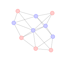
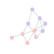
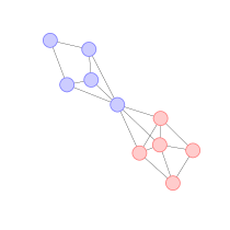
Figure 4: Planted Partition model with $n=10$ and $p+q=0.8$.
Panel A: $p=q=0.4$. Panel B: $p=0.6,q=0.2$. Panel C: $p=0.75,q=0.05$

Corollary 6.

In a planted partition model with matching probabilities $p$ and $q$, expected profits are only a function of $p+q$ and not of $p/q$.

Comparative Statics: Investing in Workers

Should a firm invest in training workers or on team building exercises? Consider an augmented version of the model with marginal cost to effort $v\geq 1$

$$\psi_{i}(\mathbf{e})=v\frac{e_{i}^{2}}{2}-\lambda e_{i}\sum_{j}g_{ji}e_{j}$$

Imagine that a firm can decrease $v$ or increase $\lambda$ at the same per-unit cost. Should a firm invest in lowering effort costs or increasing peer effects?

$$\frac{\partial\mathbb{E}(\pi)}{\partial\lambda}\lessgtr\Big{\lvert}\frac{\partial\mathbb{E}(\pi)}{\partial v}\Big{\rvert}$$

We can extend Proposition 2 to compute

$$\frac{\partial}{\partial v}\>\frac{1}{2v}\sum_{\ell}\frac{\left(\mathbf{u}_{\ell}^{\prime}\mathbf{1}\right)^{2}}{\left(1+vr\sigma^{2}\right)\left(1-\frac{\lambda}{v}\mu_{\ell}\right)^{2}-\left(\frac{\lambda}{v}\mu_{\ell}\right)^{2}}$$

and similarly w.r.t. $\lambda$

Proposition 5.

Investing uniformly in team strength (i.e. increasing $\lambda$) is superior (inferor) to investing uniformly in worker productivity (i.e. decreasing $v$) in those firms where peer networks satisfy the following condition:

$$\left(1-\mu_{\ell}\right)\left(1+r\sigma^{2}\left(v-\lambda\mu_{\ell}\right)\right)<(>)\>1/2,\>\>\ \text{for all }\ell\text{ with }\mathbf{u}_{\ell}^{\prime}\mathbf{1}\neq 0$$

From this condition you can find a threshold $\hat{d}$ such that for regular graphs with $d>\hat{d}$ investing in team strength is superior. Looking at Proposition 5 we can see that $\hat{d}\in(0,1)$. In other words, the only regular peer structure for which investing in productivity dominates is when agents don’t interact (i.e. the empty network).

The first thing to notice is that as $r\sigma^{2}$ grows, it is less profitable to invest in team-building exercises, everything else equal. Intuitively, when the cost associated to providing risky incentives increases – either because the firm is very risky or the workforce is very risk averse – performance-based compensation is costly, so investing in peer effects has little impact.

Example: regular networks, full bipartite graphs. Counter-example: empty network,

3 Coarse Instruments

We now imagine that the firm cannot write a separate contract for each worker based on their network position. Agents are exogenously sorted into $k$ types (positions or job descriptions). The Principal is now constrained to offer the same linear wage scheme for all agents in groups $k$:

$$w_{i}(X)=\beta_{k}+\alpha_{k}X\quad\forall\;i\in k$$

Thus, optimal wage schemes are decided at the type (coarsest) level, instead of the individual (granular) level.

Agents’ cost of providing effort and utility function remain unchanged. This results in the same certain equivalent and ultimately identical response functions that characterize the Nash Equilibrium (NE) previously described:

$$\mathbf{e}^{\star}=(\mathbf{I}-\lambda\mathbf{G})^{-1}\boldsymbol{\alpha}=\mathbf{C}\boldsymbol{\alpha},$$

where in this case $\alpha_{i}=\alpha_{k}\forall i\in k$.

Because the principal is now limited to type-based contracts, all $\alpha_{i}$’s and $\beta_{i}$’s are the same for the same types. To instrumentalize the coarse contracts, we introduce the linear operator $T$ as an $n\times k$ vector-diagonal matrix such that $T_{i,j}=1$ if individual $i$ belongs to type $j$ and $T_{i,j}=0$ otherwise. We next define $\hat{\alpha}$, a $k\times 1$ vector, such that $\hat{\alpha}_{k}$ is the $\alpha_{i}$ corresponding to all workers of type $k$, thus $\alpha=T\hat{\alpha}$. We define $\hat{\beta}$ analogously.

Example 2.

Take $1$ worker of type $1$, $2$ workers of type $2$, and $3$ workers of type $3$. Thus,

$$\mathbf{T}=\begin{bmatrix}1&0&0\\ 0&1&0\\ 0&1&0\\ 0&0&1\\ 0&0&1\\ 0&0&1\\ \end{bmatrix},\quad\boldsymbol{\hat{\alpha}}=\begin{bmatrix}\alpha_{1}\\ \alpha_{2}\\ \alpha_{3}\\ \end{bmatrix},\quad\boldsymbol{\alpha}=\mathbf{T}\boldsymbol{\hat{\alpha}}^{*}=\begin{bmatrix}\alpha_{1}\\ \alpha_{2}\\ \alpha_{2}\\ \alpha_{3}\\ \alpha_{3}\\ \alpha_{3}\\ \end{bmatrix}.$$

Under this setup, the Principal can no longer provide individual $\beta_{i}$’s such that the Participation Constraint (PC) of each agent binds. The participation constraints for agent $i$ considering the informational rents $\mu_{i}$ is thus:

$$\operatorname{CE}_{i}(e,G;w_{k})-\mu_{i} =0\quad\forall\;i$$

$$\mu_{i} \geq 0\quad\forall\;i$$

The key underlying assumption is that the principal ensures that all agents participate.

Linear operator $T$ together with vector $\mu$ allows us to re-write the Principal’s problem under coarsest instruments as:

$$\max_{\hat{\alpha},\hat{\beta},\mu}\mathbb{E}[\pi(X,w|e)] =\sum_{i}e_{i}-\sum_{i}w_{i}$$

subject to

$$\operatorname{CE}_{i}(e,G;w_{k})-\mu_{i} =0\quad\forall\;i\quad$$ (PC)

$$\mu_{i} \geq 0\quad\forall\;i$$

$$\mathbf{e} =(\mathbf{I}-\lambda\mathbf{G})^{-1}(\mathbf{T}\boldsymbol{\hat{\alpha}})\quad$$ (IC)

The binding participation constraint implies that the $\beta_{k}$ component of the wage for agent $i$ in group $k$ is:

$$\beta_{k}=\mu_{i}+\alpha_{k}^{2}\left(\frac{r\sigma^{2}}{2}\right)+\frac{1}{2}e_{i}^{2}-\lambda e_{i}\sum_{j}g_{ij}e_{j}-\alpha_{k}\sum_{i}e_{i}$$

By replacing $\alpha_{k}$ and $\beta_{k}$ into the problem of the principal, we can reexpress it into vector form as:

$$\max_{\hat{\alpha},\mu}\mathbb{E}[\pi(X,w|e)] =\mathbf{1}^{\prime}\mathbf{e}+\lambda\mathbf{e}^{\prime}\mathbf{G}\mathbf{e}-\frac{1}{2}\mathbf{e}^{\prime}\mathbf{e}-\frac{1}{2}r\sigma^{2}(\mathbf{T}\boldsymbol{\hat{\alpha}})^{\prime}(\mathbf{T}\boldsymbol{\hat{\alpha}})-\mathbf{1}^{\prime}\boldsymbol{\mu}$$

subject to

$$\mu_{i} \geq 0\quad\forall\;i$$

$$\mathbf{e} =(\mathbf{I}-\lambda\mathbf{G})^{-1}(\mathbf{T}\boldsymbol{\hat{\alpha}})\quad$$ (IC)

The solution to the above problem leads to the following proposition:

Proposition 6 (Coarse Contracts).

There exists a group wage function $w(\mathbf{G})=\beta_{k}+\alpha_{k}X$ with $\alpha_{k},\beta_{k}\in\mathbb{R}$, such that $w_{k}(\mathbf{G})\propto T^{\prime}B(\lambda,\mathbf{G})$. In this case, the vector of optimal sharing rules is given by:

$$\boldsymbol{\hat{\alpha}}^{*}=(\mathbf{T}^{\prime}(r\sigma^{2}\mathbf{I}+\mathbf{C}^{\prime}(\mathbf{I}-\lambda(\mathbf{G}+\mathbf{G}^{\prime}))\mathbf{C})\mathbf{T})^{-1}\mathbf{T}^{\prime}\mathbf{C}^{\prime}\boldsymbol{1}$$

Where $\mathbf{C}\equiv(\mathbf{I}-\lambda\mathbf{G})^{-1}$ is an $n\times n$ matrix such that $\mathbf{CT}\boldsymbol{\hat{\alpha}}^{*}=B_{\alpha}(\lambda,\mathbf{G})$.

In this setup, group-$k$’s centrality attributes determine the incentives provided to the whole group.

Take $\lambda=0$, then $\boldsymbol{\hat{\alpha}}^{*}=(r\sigma^{2}\mathbf{T}^{\prime}\mathbf{T}+\mathbf{T}^{\prime}\mathbf{T})^{-1}\mathbf{T}^{\prime}\mathbf{1}$ and:

$$\alpha_{i}^{\ast}=\frac{1}{1+r\sigma^{2}}.$$

As profits are globally decreasing in $\beta_{k}$, then the optimal contract requires the smallest $\beta_{k}$ to each type in a way that ensures the participation of all agents. This is achieved by considering the agent (within each type) with the highest cost of providing effort ($\psi_{i}$), thus ensuring that all agents of that type (and with lower or equal costs) are also motivated to participate:

$$\beta_{k}=\alpha_{k}^{2}\left(\frac{r\sigma^{2}}{2}\right)-\alpha_{k}\sum_{i}e_{i}+\underbrace{\max_{i\in k}{\left\{\frac{1}{2}e_{i}^{2}-\lambda e_{i}\sum_{j}g_{ij}e_{j}\right\}}}_{=\max_{i\in k}\{\psi_{i}\}}.$$

It turns out that, within each type, given the impossibility of assigning individual-based fixed wages, workers with lower effort costs will enjoy rents above their participation constraints:

$$\mu_{i}=\max_{i\in k}\left\{\frac{1}{2}e_{i}^{2}-\lambda e_{i}\sum_{j}g_{ij}e_{j}\right\}-\left\{\frac{1}{2}e_{i}^{2}-\lambda e_{i}\sum_{j}g_{ij}e_{j}\right\}\quad\forall i,k$$

$$\mu_{i}=\max_{i\in k}\{\psi_{i}\}-\psi_{i}\quad\forall i,k,$$

where $\mu_{i}$ can be interpreted as worker $i$’s centrality rents, equal to zero for the least central worker in each group. This leads to the following result:

Proposition 7 (Equilibrium Profits with Coarse Contracts).

With coarse instruments, a firm’s profits in expectation are maximized at one-half of equilibrium output minus the sum of total agent’s centrality, rents for any network $\mathbf{G}$, any level of peer effects $\lambda$, and any level fundamental risk $\sigma^{2}$.

The inefficiency of coarse instruments

Proposition 7 implies that profits are equal to half efforts minus the sum of centrality rents: $\mathbb{E}(\pi^{\star})=\frac{1}{2}X^{\star}-\sum_{i}\mu_{i}=\frac{1}{2}\sum_{i}e_{i}^{\star}-\sum_{i}\mu_{i}$. Notice that the losses associated to limiting contracts to coarse instruments (C), and compared to profits when granular contracts (G) are available, can be expressed as:

$$\pi^{G}-\pi^{C}- =\frac{1}{2}\boldsymbol{1}^{\prime}\mathbf{e}^{G}-\left(\frac{1}{2}\boldsymbol{1}^{\prime}\mathbf{e}^{C}-\boldsymbol{1}^{\prime}\boldsymbol{\mu}\right)$$

$$=\frac{1}{2}\boldsymbol{1}^{\prime}\left(\mathbf{e}^{G}-\mathbf{e}^{C}\right)+\boldsymbol{1}^{\prime}\boldsymbol{\mu}$$

$$=\frac{1}{2}\boldsymbol{1}^{\prime}\mathbf{C}\left(\boldsymbol{\alpha}^{G}-\boldsymbol{\alpha}^{C}\right)+\boldsymbol{1}^{\prime}\boldsymbol{\mu}$$

Because centrality rents are obtained through the impossibility of providing individual-based betas, then losses associated with coarse instruments can be divided into losses due to difference in the $\boldsymbol{\alpha}$ and the $\boldsymbol{\beta}$ components. We explore this effects in the next section by conducting simulations on different random graphs.

3.1 Simulations

To illustrate the implications of providing group-based contracts instead of individual-based wage schemes, we simulate a different random networks using an Erdős-Rényi network generating process, with parameter $p_{ER}\in[0,1]$. We compute then the optimal contract for each network assuming individual-based contracts and then assuming that the whole network is subject to the same wage scheme (i.e., they all belong in the same type).

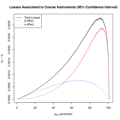
Figure 5: Components of Difference in Profits for different $p_{ER}$

Figure 5 showcases the effect of coarsen wage contracts and its implications for different random network. In Figure 5, the blue line represent the $\boldsymbol{\alpha}$ component of losses (i.e., $\frac{1}{2}\boldsymbol{1}^{\prime}\mathbf{C}\left(\boldsymbol{\alpha}^{G}-\boldsymbol{\alpha}^{C}\right)$), while the red line display the losses associated to centrality rents ($\boldsymbol{\beta}$ component). The black line are total losses, computed as the sum of both effects.

First, notice that losses vanish in the extreme cases of the Erdős-Rényi network generation process: the empty and full networks. Moreover, notice that the $\alpha$ effect plays a smaller role in overall losses as the network grows denser, while the $\beta$ effect peaks closer to the full network, before vanishing when the network becomes fully connected. This suggests that certain network structures are more disadvantageous when Principals are limited to provide wage contracts that do not discriminate across employees. The relationship between degree and centrality distributions and losses associated to coarse instruments is a subject of study for later versions of this paper.

4 Modular Production

So far, we have assumed that expected output is a linear function of workers’ efforts. Therefore, while workers may inhabit very different parts of the peer network, we assumed that their formal role within the organization is substitutable. This allowed us to conveniently isolate the impact of peer effects on wages and profits, but it fails to capture that a firm’s production function may actually drive its organization.

Today many products are made by assembling separately-produced components, all of which are essential constituents of the final good. Partitioning firm production into separable elements can generate superior, more versatile products, as IBM uncovered when they developed the first modular computer in 1964. But failures in any one module can also affect overall production. In an extreme example popularized by Kremer (1993), the Challenger spacecraft exploded in 1984 because one of its many components, the O-ring, malfunctioned. In this section we consider how incentive contracts with peer complementarities are designed in firms that have fragmented organizational structures.

To do this we modify our production function by incorporating modules and assume that final output is determined by the weakest-performing module. Formally, assume that $N$ workers are distributed into $K$ teams, called $k_{1},k_{2},\ldots,k_{K}$, each of which is put in charge of designing a separate module. Within a team, performance is substitutable but across teams it is perfectly complementary. We now write firm output as,

$$X(\mathbf{e})=\min\{\sum_{i\in k_{1}}e_{i},\sum_{i\in k_{2}}e_{i},\ldots,\sum_{i\in k_{K}}e_{i}\}+\varepsilon$$ (8)

Notice that our original production function is a specific instance of (8) for the case in which all workers are contained in one single module. How should incentives contracts be designed under modular production? And how it will depend on the network of spillovers within and across teams?

For any linear incentive contract, $(\alpha_{i},\beta_{i})_{i\in N}$, there are now multiple equilibria of the effort provision game played by workers. For example, everyone playing $e_{i}=0$ is always an equilibrium. Secondly, notice that in any equilibrium each module will exert the same total effort because a worker whose team contributes more than the weakest module will gain from reducing her effort. Therefore $\sum_{i\in k}e_{i}=\hat{e}$ for all modules $k\in K$, and some $\hat{e}\geq 0$. The question now is which values of $\hat{e}$ constitute a Nash equilibrium? Imagine that every team is contributing $\hat{e}$ and consider if a worker could profitably deviate. Given technology (8), a worker can never gain by increasing effort. Decreasing effort, however, is profitable as long as the marginal cost to lowering $e_{i}$ (given by $\alpha_{i}$) is less than the marginal benefit: $e_{i}-\lambda\sum_{j}g_{ij}e_{j}$. This implies that in any equilibirum all teams exert the same effort $\hat{e}$ and the following condition holds:

$$\alpha_{i}\geq e_{i}-\lambda\sum_{j}g_{ij}e_{j}\quad\forall i\in N.$$

Now, although there are many values of $\hat{e}$ that constitute an equilibrium, we focus in this section on the maximal equilibrium: given any choice of $\boldsymbol{\alpha}$ by the firm, there will be a value of $\overline{e}(\boldsymbol{\alpha})$ that constitutes a Nash equilibrium of the game, such that any $\hat{e}>\overline{e}$ is not a Nash equilibrium. Moreover, notice that if the above inequality is strict for any worker $i$, the firm can always lower $\alpha_{i}$ without affecting anyone’s behavior. Since the firm always prefers the lowest $\boldsymbol{\alpha}$ that guarantees a specific $\overline{e}$, we can conclude that the following two conditions must always hold in any optimal contract under modular production

1. $\alpha_{i}=e_{i}-\lambda\sum_{j}g_{ij}e_{j},\>\>\forall i\in N$.

2. $\overline{e}(\boldsymbol{\alpha})=\sum_{i\in k}e_{i},\>\>\forall k\in K$

The first

Define the matrix $\mathbf{M}_{k\times n}$, such that $\mathbf{M}_{ki}=1$ if agent $i$ is part of module $k$, and zero otherwise. Then,

$$\mathbf{M}\mathbf{e}=\hat{e}\boldsymbol{1_{k}},$$

where $\boldsymbol{1_{k}}$ denotes a vector ones of lenght $k$ (in the previous case of individual modules, we had that $\mathbf{M}=\mathbf{I}$ and thus the simplified case of $\mathbf{e}=\hat{e}\boldsymbol{1}$).

Example 3.

Take workers $1-3$ belonging in module $1$ and workers $4-5$ belonging in module $2$. Then,

$$\mathbf{M}=\begin{bmatrix}1&1&1&0&0\\ 0&0&0&1&1\\ \end{bmatrix},\quad\hat{e}\boldsymbol{1_{k}}=\begin{bmatrix}\hat{e}\\ \hat{e}\\ \end{bmatrix},\quad\mathbf{M}\mathbf{e}=\begin{bmatrix}\sum_{i\in[1,3]}e_{i}\\ \sum_{i\in[4,5]}e_{i}\\ \end{bmatrix}=\begin{bmatrix}\hat{e}\\ \hat{e}\\ \end{bmatrix}.$$

Take the principal constrained maximization problem:

$$\max_{(\hat{e},\boldsymbol{\alpha})}\left(\hat{e}-\frac{1}{2}\mathbf{e}^{\prime}(\mathbf{I}-2\lambda\mathbf{G})\mathbf{e}-\frac{\sigma^{2}r}{2}\boldsymbol{\alpha}^{\prime}\boldsymbol{\alpha}\right)$$

subject to

$$\mathbf{e}=\mathbf{C}\boldsymbol{\alpha}$$

$$\mathbf{M}\mathbf{e}=\hat{e}\boldsymbol{1_{k}}$$

Take as a concrete example the case where every worker makes up a separate module. In that case With this we arrive at the following result

Corollary 7.

When modules are of size $1$ incentives are assigned based on the number of connections across modules

$$\alpha_{i}^{*}=\frac{1-\lambda d_{i}}{\sum_{i}\left(1-2\lambda d_{i}\right)+\sigma^{2}r\left(1-\lambda d_{i}\right)^{2}}$$

.

5 Discussion

We offer valuable insights into the dynamics of optimal wage design in organizations with productivity spillovers. By analyzing the interplay between individual effort, network centrality, and group composition, we have provided a framework for designing efficient wage contracts that balance incentives and risk mitigation. Our findings underscore the importance of considering both individual and group-level factors when determining optimal wage structures, highlighting the significance of network centrality in targeting incentives effectively.

Moreover, our research highlights the trade-offs involved in wage discrimination based on network position, revealing how firms can extract surplus while accommodating workers’ risk exposure. The distinction between individualized and group-based contract designs sheds light on the strategic decisions firms face in optimizing their organizational structure. By elucidating these complexities, our study contributes to the literature on incentive design and organizational economics, offering practical implications for firms seeking to enhance productivity and profitability in collaborative work environments.

Appendix A Proofs

A.1 Proof of Proposition 1

Notice that the principal’s problem can be written in matrix form as:

$$\max_{\boldsymbol{\alpha}}\>\mathbb{E}[\pi(\mathbf{e}\mid\boldsymbol{\alpha},\boldsymbol{\beta})]$$

subject to

$$\mathbf{e}^{\star}=\mathbf{C}\boldsymbol{\alpha}\quad$$ (IC)

With $\mathbf{C}\equiv(I-\lambda\mathbf{G})^{-1}$ depending exclusively on given parameters. Using the (IC), we can rewrite the problem as:

$$\max_{\boldsymbol{\alpha}}\>\mathbb{E}[\pi(\mathbf{e}\mid\boldsymbol{\alpha},\boldsymbol{\beta})]=\boldsymbol{\alpha}^{\prime}\mathbf{C}^{\prime}\mathbf{1}-\frac{1}{2}\boldsymbol{\alpha}^{\prime}\mathbf{C}^{\prime}\mathbf{C}\boldsymbol{\alpha}+\lambda\boldsymbol{\alpha}^{\prime}\mathbf{C}^{\prime}\mathbf{G}\mathbf{C}\boldsymbol{\alpha}-\frac{1}{2}\sigma^{2}r\boldsymbol{\alpha}^{\prime}\boldsymbol{\alpha}$$

The first-order conditions with respect to $\boldsymbol{\alpha}$ imply:

$$0 =\mathbf{C}^{\prime}\boldsymbol{1}-\mathbf{C}^{\prime}\mathbf{C}\boldsymbol{\alpha}^{\star}+\lambda\mathbf{C}^{\prime}(\mathbf{G}+\mathbf{G}^{\prime})\mathbf{C}\boldsymbol{\alpha}^{\star}-\sigma^{2}r\boldsymbol{\alpha}^{\star}$$

$$\Rightarrow\boldsymbol{\alpha}^{\star} =\left(\mathbf{C}^{\prime}(\mathbf{I}-\lambda(\mathbf{G}+\mathbf{G}^{\prime}))\mathbf{C}+\sigma^{2}r\mathbf{I}\right)^{-1}\mathbf{C}^{\prime}\mathbf{1}$$

$$=\left(\mathbf{C}-\mathbf{I}-\lambda\mathbf{C}^{\prime}\mathbf{G}\mathbf{C}+(1+\sigma^{2}r)\mathbf{I})\right)^{-1}\mathbf{C}^{\prime}\mathbf{1}$$

$$=\left(\lambda\mathbf{G}\mathbf{C}-\lambda\mathbf{C}^{\prime}\mathbf{G}\mathbf{C}+(1+\sigma^{2}r)\mathbf{I}\right)^{-1}\mathbf{C}^{\prime}\mathbf{1}$$

$$=\left((1+\sigma^{2}r)\mathbf{I}-\lambda(\mathbf{C}^{\prime}-\mathbf{I})\mathbf{G}\mathbf{C}\right)^{-1}\mathbf{C}^{\prime}\mathbf{1}$$

$$\boldsymbol{\alpha}^{\star} =\left((1+\sigma^{2}r)\mathbf{I}-\lambda^{2}(\mathbf{C}\mathbf{G})^{\prime}\mathbf{G}\mathbf{C}\right)^{-1}\mathbf{C}^{\prime}\mathbf{1}$$

Where the last step follows from $\mathbf{G}\mathbf{C}=\mathbf{G}+\lambda\mathbf{C}^{2}+\lambda^{3}\mathbf{C}^{3}+...=\frac{1}{\lambda}(\mathbf{C}-\mathbf{I})$ and $\mathbf{G}^{\prime}\mathbf{C}^{\prime}=\frac{1}{\lambda}(\mathbf{C}^{\prime}-\mathbf{I})$. Finally, we have that:

$$\beta_{i}(\boldsymbol{\alpha},\mathbf{e})=\frac{1}{2}e_{i}^{2}-\lambda e_{i}\sum_{j}g_{ij}e_{k}+\alpha_{i}^{2}\frac{r\sigma^{2}}{2}-\alpha_{i}\sum_{k}e_{k}$$

and thus:

$$\beta^{\star}(\boldsymbol{\alpha}^{\star},\mathbf{e}^{\star})=\frac{1}{2}(\mathbf{e}^{\star}\circ\mathbf{e}^{\star})-(\mathbf{e}^{\star}\circ\lambda\mathbf{G}\mathbf{e}^{\star})+\frac{1}{2}(r\sigma^{2})(\boldsymbol{\alpha}^{\star}\circ\boldsymbol{\alpha}^{\star})-\boldsymbol{\alpha}^{\star}\circ\mathbf{1}(\mathbf{1}^{\prime}\mathbf{e}^{\star})$$

where $\circ$ denotes the Hadamard, element-wise, product.

As $\mathbf{e}^{\star}=\mathbf{C}\boldsymbol{\alpha}^{\star}$, the above can be re-expressed as

$$\beta^{\star}(\boldsymbol{\alpha}^{\star})=\frac{1}{2}\left[\mathbf{C}\boldsymbol{\alpha}^{\star}\circ\left(\mathbf{I}-2\lambda\mathbf{G}\right)\mathbf{C}\boldsymbol{\alpha}^{\star}+\boldsymbol{\alpha}^{\star}\circ\left(r\sigma^{2}\mathbf{I}-2\mathbf{1}\mathbf{1}^{\prime}\mathbf{C}^{\prime}\right)\boldsymbol{\alpha}^{\star}\right]$$

A.2 Proof of Proposition 2

Suppose worker $i$ has a higher Bonacich centrality than worker $j$. Then,

$$\left(\mathbf{C1}\right)_{i}>\left(\mathbf{C1}\right)_{j}\Rightarrow\left(\mathbf{C1}\right)_{i}-1>\left(\mathbf{C1}\right)_{j}-1\Rightarrow\left((\mathbf{C}-\mathbf{I})1\right)_{i}>\left((\mathbf{C}-\mathbf{I})1\right)_{j}.$$

Notice that

$$\mathbf{C}\lambda\mathbf{G}=\sum_{k=1}^{\infty}(\lambda\mathbf{G})^{k}=(\mathbf{C}-\mathbf{I}).$$

Thus,

$$\left(\mathbf{C1}\right)_{i}>\left(\mathbf{C1}\right)_{j}\Rightarrow((\lambda\mathbf{G})\mathbf{C1})_{i}>((\lambda\mathbf{G})\mathbf{C1})_{j}$$

Thus, $\lambda\mathbf{G}$ is an order-preserving transformation of $\mathbf{C1}=\mathbf{B}$, the vector of Bonacich centralities. In other words, multiplying $\lambda\mathbf{G}$ times $\mathbf{C1}$ gives a vector $\mathbf{\tilde{B}}$ with the same order as the vector of Bonacich centralities $\mathbf{B}$. Then, multiplying $\lambda\mathbf{G}$ times $\mathbf{\tilde{B}}$ also preserves the order of the vector $\mathbf{B}$. More generally, $(\lambda\mathbf{G})^{k}\mathbf{C1}=(\lambda\mathbf{G})^{k}\mathbf{B}$ and preserves the order of $\mathbf{B}$. Therefore,

$$\mathbf{CB}=\mathbf{B}+\lambda\mathbf{GB}+(\lambda\mathbf{G})^{2}\mathbf{B}+\cdots$$

also preserves the order of $\mathbf{B}$ as well as $\lambda\mathbf{GCB}$ and $[(\lambda\mathbf{GC})\lambda\mathbf{GC}]\mathbf{B}$. Thus,

$$\gamma(\mathbf{I}+[(\lambda\mathbf{GC}\lambda\mathbf{GC})+[(\lambda\mathbf{GC})\lambda\mathbf{GC}]^{2}+\cdots])\mathbf{B}=\gamma(\mathbf{I}-[(\lambda\mathbf{GC})\lambda\mathbf{GC}])^{-1}\mathbf{B}$$

where $\gamma=1/(1+r\sigma^{2})$, also preserves the order of $\mathbf{B}$. Finally, this implies that,

$$\gamma(\mathbf{I}-[(\lambda\mathbf{GC})\lambda\mathbf{GC}])^{-1}\mathbf{B}=\frac{1}{1+r\sigma^{2}}\left(\mathbf{I}-\frac{\lambda^{2}}{1+r\sigma^{2}}(\mathbf{GC})\mathbf{GC}\right)^{-1}\mathbf{B}=\mathbf{WB}=\boldsymbol{\alpha}.$$

A.3 Proof of Proposition 3

Recall that the optimal performance-based compensation is given by

$$\boldsymbol{\alpha}^{\star}=\frac{1}{1+r\sigma^{2}}\left[\mathbf{I}-\frac{\lambda^{2}}{1+r\sigma^{2}}(\mathbf{CG})^{\prime}\mathbf{C}\mathbf{G}\right]^{-1}\mathbf{C^{\prime}1}$$

Part 1. Showing that the derivative of the vector of optimal performance-based compensation with respect to the intensity of the link from worker $i$ to worker $j$ is non-negative.

Using the chain rule and letting $\mathbf{W}=[\mathbf{I}-\frac{\lambda^{2}}{1+r\sigma^{2}}(\mathbf{CG})^{\prime}\mathbf{C}\mathbf{G}]^{-1}$, we can write the derivative with respect to $g_{ij}$ as the sum of two terms:

$$\frac{\partial\boldsymbol{\alpha}^{*}}{\partial g_{ij}}=\frac{1}{1+r\sigma^{2}}\left[\frac{\partial\mathbf{W}}{\partial g_{ij}}\cdot\mathbf{C^{\prime}1}+\mathbf{W}\cdot\frac{\partial\mathbf{C^{\prime}1}}{\partial g_{ij}}\right].$$ (9)

Focus on the derivative of the inverse matrix:

$$\frac{\partial\mathbf{W}}{\partial g_{ij}}=-\mathbf{W}\frac{\partial[\mathbf{I}-\frac{\lambda^{2}}{1+r\sigma^{2}}(\mathbf{CG})^{\prime}\mathbf{C}\mathbf{G}]}{\partial g_{ij}}\mathbf{W}=\frac{\lambda^{2}}{1+r\sigma^{2}}\mathbf{W}\frac{\partial\mathbf{G^{\prime}C^{\prime}CG}}{\partial g_{ij}}\mathbf{W}.$$

Applying the chain rule a few more times, and noticing that the derivatives of $\mathbf{G}$ and $\mathbf{C}$ are

$$\frac{\partial\mathbf{G}}{\partial\mathbf{g_{ij}}}=\mathbf{E_{ij}}\quad\text{and}\quad\frac{\partial\mathbf{C}}{\partial g_{ij}}=\lambda\mathbf{C}\mathbf{E_{ij}}\mathbf{C},$$

where $\mathbf{E_{ij}}$ is a matrix of all zeros except element $(i,j)$ is equal to one, we can write the first term in the brackets of (9) as

$$\frac{\partial\mathbf{W}}{\partial g_{ij}}\cdot\mathbf{C^{\prime}1}=\frac{\lambda^{2}}{1+r\sigma^{2}}\mathbf{W}\left[\mathbf{E_{ji}}\mathbf{C^{\prime}CG}+\lambda\mathbf{G^{\prime}C^{\prime}}(\mathbf{E_{ji}}\mathbf{C^{\prime}CG}+\mathbf{C}\mathbf{E_{ij}}\mathbf{CG)+\mathbf{G^{\prime}C^{\prime}C}\mathbf{E_{ij}}}\right]\mathbf{W}\cdot\mathbf{C^{\prime}1},$$ (10)

which is non-negative because all matrices are non-negative. Next, focus on the second term in brackets of (9). The entry $s$ of the derivative vector of $\mathbf{C^{\prime}1}$ with respect to $g_{ij}$ is given by

$$\frac{\partial(\mathbf{C^{\prime}1})_{s}}{\partial g_{ij}}=\frac{\partial\sum_{t=1}^{n}c_{ts}}{\partial g_{ij}}=\sum_{t=1}^{n}\frac{\partial c_{ts}}{\partial g_{ij}}=\sum_{t=1}^{n}\lambda m_{ti}m_{js}=\lambda m_{js}\sum_{t=1}^{n}m_{ti},$$

where the second equality follows from taking the $(t,s)$ element of the derivative of $\mathbf{C}$ with respect to $g_{ij}$. Note that the derivative above is positive if $c_{js}>0$, i.e., if worker $j$ is influenced by worker $s$. Moreover, when $s=j$ this derivative is always strictly greater than zero. Thus, the second term in the brackets of (9) is

$$\mathbf{W}\cdot\frac{\partial\mathbf{C^{\prime}1}}{\partial g_{ij}}=\left(\lambda\sum_{t=1}^{n}c_{ti}\right)\mathbf{W}\cdot\begin{bmatrix}c_{j1}\\ \vdots\\ c_{jn}\end{bmatrix}\geq 0.$$

Part 2. Show that for agents $k$ not weakly connected to $j$, the derivative of $\alpha_{k}^{*}$ with respect to $g_{ij}$ is zero.

We have that

$$\frac{\partial\alpha_{k}^{*}}{\partial g_{ij}}=\frac{1}{1+r\sigma^{2}}\sum_{l=1}^{n}\left[\frac{\partial\omega_{kl}}{\partial g_{ij}}\cdot(\mathbf{C^{\prime}1})_{l}+\omega_{kl}\cdot\frac{\partial(\mathbf{C^{\prime}1})_{l}}{\partial g_{ij}}\right].$$ (11)

Without loss of generality, it is convenient to relabel workers so that those weakly connected to worker $j$ are workers $s\in\{1,2,\dots,i\}$, and those weakly connected to $k$, who is not weakly connected to $j$, are $r\in\{l,\dots,n\}$. Thus, we have that $A=\{1,2,\dots,i\}\cup\{j,k\}\cup\{l,\dots,n\}$. This relabeling of workers allows us to treat $\mathbf{G}and\mathbf{C}$ as block matrices:

$$\mathbf{G}=\begin{pmatrix}{\mathbf{G_{j}}}&\vline&\mathbf{0_{j}}\\ \hline\cr\mathbf{0_{k}}&\vline&\mathbf{G_{k}}\end{pmatrix}\quad\text{and}\quad\mathbf{C}=\begin{pmatrix}\mathbf{C_{j}}&\vline&\mathbf{0_{j}}\\ \hline\cr\mathbf{0_{k}}&\vline&\mathbf{C_{k}}\end{pmatrix},$$

where $\mathbf{G_{j}}$ and $\mathbf{G_{k}}$ are $j\times j$ and $(n-j)\times(n-j)$ matrices that only involve direct and indirect neighbors of $j$ and $k$, respectively, $\mathbf{C_{j}}$ and $\mathbf{C_{k}}$ are $j\times j$ and $(n-j)\times(n-j)$ matrices that capture the account for the total weight of all walks in each weakly connected component, and $\mathbf{0_{j}}$ and $\mathbf{0_{k}}$ are $j\times(n-j)$ and $(n-j)\times j$ matrices of zeros. Notice that each non-zero block in $\mathbf{G}$ and $\mathbf{C}$ can have some zero entries and is not necessarily symmetric. By (7), for any $x\geq 0$, the product $((\mathbf{CG})^{\prime}\mathbf{CG})^{x}$ results in a symmetric matrix with the same block-structure, i.e., blocks $(1,2)$ and $(2,1)$ are both zero matrices. Thus, we can write $\mathbf{W}$ as

$$\mathbf{W}=\begin{pmatrix}\mathbf{W_{j}}&\vline&\mathbf{0_{j}}\\ \hline\cr\mathbf{0_{k}}&\vline&\mathbf{W_{k}}\end{pmatrix}$$

where $\mathbf{W_{j}}$ and $\mathbf{W_{k}}$ are $j\times j$ and $(n-j)\times(n-j)$ matrices capturing common influences between pairs of workers. Because $\mathbf{W}$ can be written as a block-diagonal matrix, we know that $\omega_{ks}=0$ for all $s\in\{1,\dots,i\}\cup\{j\}$. Moreover, the derivative of $(\mathbf{C^{\prime}1})_{r}$ with respect to $g_{ij}$, computed in part 1, is always zero since $c_{jr}=0$ for all $r\in\{l,\dots,n\}\cup\{k\}$. That is, for all $s\in\{1,\dots,i\}\cup\{j\}$, the second term in (11) is zero by $\omega_{ks}=0$, and for all $r\in\{l,\dots,n\}\cup\{k\}$, the second term in (11) is zero by $\partial(\mathbf{C^{\prime}1})_{r}/\partial g_{ij}=0$. Thus, the second term in (11) is equal to zero for all workers. Because $\omega_{ks}=0$ for all $s\in\{1,\dots,i\}\cup\{j\}$, the derivative in the first term in (11) is equal to zero. It remains to show that same term is equal to zero for all $r\in\{l,\dots,n\}$. To see this, notice we can write the matrix $\mathbf{E_{ij}}$ in (10) as a block matrix:

$$\mathbf{E_{ij}}=\begin{pmatrix}\mathbf{E_{ij}}&\vline&\mathbf{0_{j}}\\ \hline\cr\mathbf{0_{k}}&\vline&\mathbf{0_{kk}}\end{pmatrix}$$

, where $\mathbf{0_{kk}}$ is a $(n-j)\times(n-j)$ matrix of zeros. Then, multiplying this matrix, or its transpose $\mathbf{E_{ji}}$, by the block matrices $\mathbf{C}$ or $\mathbf{C}^{T}$ will result in a block matrix with $\mathbf{0_{kk}}$ in the $(2,2)$ block. This implies that $\partial\omega_{kr}/\partial g_{ij}$ is equal to zero for all $r=\{l,\dots,n\}\cup\{k\}$. This establishes that an increase in $g_{ij}$ has no effect on the optimal performance-related compensation of workers that are not weakly connected to $j$.

Part 3. Showing that for workers weakly connected to $j$, they must have at least one in-link for the derivative to be strictly positive.

Consider a worker $s\in\{1,\dots,i\}$ that is weakly connected to $j$. Since $\omega_{sl}=0$ for $l\in\{k,l,\dots,n\}$, the only terms that could be positive in (11) are

$$\frac{\partial\alpha^{*}_{s}}{\partial g_{ij}}=\frac{1}{1+r\sigma^{2}}\sum_{l\in\{1,\dots,s,\dots,j\}}\left[\frac{\partial\omega_{sl}}{\partial g_{ij}}\cdot(\mathbf{C^{\prime}1})_{l}+w_{sl}\cdot\frac{\partial(\mathbf{C^{\prime}1})_{l}}{\partial g_{ij}}\right].$$ (12)

Suppose there is no $l\neq s$ such that $s$ has influence on $l$, i.e., $c_{ls}=0$ for all $l\neq s$. This implies that column $s$ of $\mathbf{G}_{j}$ and row $s$ of $\mathbf{G}^{T}$ are full of zeros. Moreover, column $s$ of $\mathbf{C}_{j}$ and row $s$ of $\mathbf{C}_{j}^{T}$ are also full of zeros except for entry $(s,s)$ which is equal to one. For any $x\geq 1$, the product $((\mathbf{C}_{j}\mathbf{G}_{j})^{T}\mathbf{C}_{j}\mathbf{G}_{j})^{x}$ results in a matrix in which row $s$ is full of zeros. Therefore, row $s$ and column $s$ of $\mathbf{W}_{j}$ are full of zeros except for the diagonal entry $(s,s)$ which is equal to one, since for $x=0$ we have that $\mathbf{W}_{j}=\mathbf{I}_{j}$. That is, if $m_{ls}=0$ for all $l\in\{1,\dots,s,\dots,j\}$, then $\omega_{sl}=0$ for all $l\neq s$ and $\omega_{ss}=1$. Thus, (12) is equal to zero if agent $s$ has no influence on any other agent, i.e., there is no agent $s^{\prime}$ for which $g_{s^{\prime}s}>0$.

Suppose that there is one $l\neq s$ such that $s$ has influence on $l$, i.e., $c_{ls}>0$. This implies that $l$ has no influence on any agent, i.e., $c_{s^{\prime}l}=0$ for all $s^{\prime}\in\{1,\dots,i,j\}$. Then, column $s$ and $l$ of $\mathbf{G}_{j}$ are all zeros except for entry $(l,s)$. Because $l$ has no influence on any other agent, columns $s$ and $l$ of $\mathbf{C}_{j}$ are full of zeros except for entries $(s,s)$, $(l,s)$, and $(l,l)$. Notice that since $l$ has no influence on any other agent, we know that $w_{s^{\prime}l}=w_{ls^{\prime}}=0$ for all $s^{\prime}\in\{1,\dots,i,j\}$ and $\omega_{ll}=1$. Because $s$ is weakly connected to $j$ and has an influence on $l$, it must be that there is some other agent $s^{\prime\prime}$ that has an influence on $l$. Thus, entry $\omega_{s,s^{\prime\prime}}$ will be positive. Since $s^{\prime\prime}$ is weakly connected to $j$, it must be that either $c_{js^{\prime\prime}}>0$ or that $c_{s^{\prime\prime}j}>0$ (or both). If the former is true, then $\omega_{ss^{\prime\prime}}>0$, and the second term in the brackets of (12) is positive for $l=s^{\prime\prime}$. If the latter is true, then $\omega_{sj}>0$, and the first term in the brackets of eq. 12 is positive for $l=j$. Either way, eq. 12 is strictly positive.

A.4 Proof of Proposition 4

We first show that a firm’s profits are maximized at one-half of equilibrium output. Recall that:

$$\boldsymbol{\alpha}^{\star}=\left[\mathbf{C}(\mathbf{I}-2\lambda\mathbf{G})\mathbf{C}+\sigma^{2}\mathbf{rI}\right]^{-1}\mathbf{C}\mathbf{1},$$

and

$$E[\pi] =\boldsymbol{\alpha}^{{}^{\prime}\,}\mathbf{C}\mathbf{1}-\frac{1}{2}\boldsymbol{\alpha}^{{}^{\prime}\,}\mathbf{C}\mathbf{C}\boldsymbol{\alpha}+\lambda\boldsymbol{\alpha}^{{}^{\prime}\,}\mathbf{C}\mathbf{G}\mathbf{C}\boldsymbol{\alpha}-\frac{1}{2}\sigma^{2}\mathbf{r}\boldsymbol{\alpha}^{{}^{\prime}\,}\boldsymbol{\alpha}$$

$$=\boldsymbol{\alpha}^{{}^{\prime}\,}\mathbf{C}\mathbf{1}-\frac{1}{2}\boldsymbol{\alpha}^{{}^{\prime}\,}\left[\mathbf{C}(\mathbf{I}-2\lambda\mathbf{G})\mathbf{C}+\sigma^{2}\mathbf{rI}\right]\boldsymbol{\alpha}.$$

Thus,

$$E[\pi^{*\,^{\prime}}] =\boldsymbol{\alpha}^{*\,^{\prime}}\mathbf{C}\mathbf{1}-\frac{1}{2}\boldsymbol{\alpha}^{*\,^{\prime}}\left[\mathbf{C}(\mathbf{I}-2\lambda\mathbf{G})\mathbf{C}+\sigma^{2}\mathbf{rI}\right]\underbrace{\left[\mathbf{C}(\mathbf{I}-2\lambda\mathbf{G})\mathbf{C}+\sigma^{2}\mathbf{rI}\right]^{-1}\mathbf{C}\mathbf{1}}_{=\boldsymbol{\alpha}^{\star}}$$

$$=\boldsymbol{\alpha}^{*\,^{\prime}}\mathbf{C}\mathbf{1}-\frac{1}{2}\boldsymbol{\alpha}^{*\,^{\prime}}\mathbf{C}\mathbf{1}$$

$$=\frac{1}{2}\boldsymbol{\alpha}^{*\,^{\prime}}\mathbf{C}\mathbf{1}$$

$$=\frac{1}{2}\mathbf{e}^{*\,^{\prime}}\mathbf{1}.$$

And therefore, $E[\pi^{\star}]=\frac{1}{2}\mathbf{X}^{\star}$.

We now prove the second part of the proposition. We first do the proof for symmetric $\mathbf{G}$. Following Proposition 1, we can write the worker’s equilibrium condition as

$$\mathbf{e}^{\star}=\mathbf{C}\boldsymbol{\alpha}=\mathbf{C}(2\mathbf{I}-\mathbf{C}+\mathbf{C}^{-1}r\sigma^{2})^{-1}\mathbf{1}$$

Rewriting, we have that

$$\left(2\mathbf{C}^{-1}-\mathbf{I}+r\sigma^{2}\mathbf{C}^{-2}\right)\mathbf{e}^{\star}=\mathbf{1}\implies\left(\mathbf{I}-2\lambda\mathbf{G}+r\sigma^{2}(\mathbf{I}-\lambda\mathbf{G})^{2}\right)\mathbf{e}^{\star}=\mathbf{1}$$

Assuming that $\mathbf{G}$ is symmetric, we have $\mathbf{G}=\mathbf{U\Sigma U}^{\prime}$ where $\mathbf{U}=(\mathbf{u}_{1},\mathbf{u}_{2},\ldots,\mathbf{u}_{n})$ is a matrix of unit-eigenvectors of $\mathbf{G}$, while $\mathbf{\Sigma}=\operatorname{diag}(\mu_{1},\mu_{2},\ldots,\mu_{n})$ is a diagonal matrix of corresponding eigenvalues. We can therefore write

$$\left(\mathbf{I}-2\lambda\mathbf{U\Sigma U}^{\prime}+r\sigma^{2}(\mathbf{I}-\lambda\mathbf{U\Sigma U}^{\prime})^{2}\right)\mathbf{e}^{\star}=\mathbf{1}$$

multiplying both sides on the left by $\mathbf{U}^{\prime}$ and factoring we have

$$\left((1+r\sigma^{2})(\mathbf{I}-2\lambda\mathbf{\Sigma})+r\sigma^{2}\lambda^{2}\mathbf{\Sigma}^{2}\right)\mathbf{U}^{\prime}\mathbf{e}^{\star}=\mathbf{U}^{\prime}\mathbf{1}$$

which means that we can write

$$\mathbf{e}^{\star}=\mathbf{U}\left((1+r\sigma^{2})(\mathbf{I}-2\lambda\mathbf{\Sigma})+r\sigma^{2}\lambda^{2}\mathbf{\Sigma}^{2}\right)^{-1}\mathbf{U}^{\prime}\mathbf{1}$$

where, conveniently,

$$\left((1+r\sigma^{2})(\mathbf{I}-2\lambda\mathbf{\Sigma})+r\sigma^{2}\lambda^{2}\mathbf{\Sigma}^{2}\right)^{-1}=$$

$$\operatorname{diag}\left(\frac{1}{(1+r\sigma^{2})(1-2\lambda\mu_{1})+r\sigma^{2}(\lambda\mu_{1})^{2}},\ldots,\frac{1}{(1+r\sigma^{2})(1-2\lambda\mu_{n})+r\sigma^{2}(\lambda\mu_{n})^{2}}\right)$$

and $\mathbf{U}^{\prime}\mathbf{1}=(\mathbf{u}_{1}^{\prime}\mathbf{1},\mathbf{u}_{2}^{\prime}\mathbf{1},\ldots,\mathbf{u}_{n}^{\prime}\mathbf{1})^{\prime}$. This means that we can write worker $i$’s equilibrium effort as a function of the graph’s spectral properties. Letting $u_{\ell,i}$ represent the $i$th element of vector $\mathbf{u}_{\ell}$, we have

$$e_{i}^{\star}=\sum_{\ell}\frac{u_{\ell,i}\left(\sum_{i}u_{\ell,i}\right)}{(1+r\sigma^{2})(1-2\lambda\mu_{\ell})+r\sigma^{2}(\lambda\mu_{\ell})^{2}}$$

Finally, combining this expression with our result stating that $\mathbb{E}(\pi^{\star})=\frac{1}{2}\sum_{i}e_{i}^{\star}$ gives our final result.

Now consider the case of directed networks. This means we can no longer assume that $\mathbf{G}$ is symmetric. However, we continue to assume that $\mathbf{G}$ is diagonalizable (i.e. all eigenvectors are linearly independent). In other words, we now have $\mathbf{G}=\mathbf{U\Sigma U}^{-1}$, where $\mathbf{U}^{-1}=(\mathbf{v}_{1},\ldots,\mathbf{v}_{n})$ is the matrix of left eigenvectors of $\mathbf{G}$. Following similar steps we arrive at the following generalized expression for profits

$$\mathbb{E}(\pi^{\star})=\frac{1}{2}\sum_{\ell}\frac{(\mathbf{v}_{\ell}^{\prime}\mathbf{1})(\mathbf{u}_{\ell}^{\prime}\mathbf{1})}{(1+r\sigma^{2})(1-2\lambda\mu_{\ell})+r\sigma^{2}(\lambda\mu_{\ell})^{2}}$$

A.5 Proof of Proposition 6

We aim to maximize:

$$\max_{\hat{\alpha},\mu}\mathbb{E}[\pi(X,w|e)] =\mathbf{e}^{\prime}\mathbf{1}+\lambda\mathbf{e}^{\prime}\mathbf{G}\mathbf{e}-\frac{1}{2}\mathbf{e}^{\prime}\mathbf{e}-\frac{1}{2}r\sigma^{2}(\mathbf{T}\boldsymbol{\hat{\alpha}})^{\prime}(\mathbf{T}\boldsymbol{\hat{\alpha}})-\mathbf{1}^{\prime}\mathbf{\mu}$$

subject to

$$\mu_{i} \geq 0\quad\forall\;i$$

$$e =(\mathbf{I}-\lambda\mathbf{G})^{-1}(\mathbf{T}\boldsymbol{\hat{\alpha}})\quad \text{(IC)}.$$

Replacing $\mathbf{e}=(\mathbf{I}-\lambda\mathbf{G})^{-1}(\mathbf{T}\boldsymbol{\hat{\alpha}})=\mathbf{C}\mathbf{T}\boldsymbol{\hat{\alpha}}$ eliminates the IC, reducing the problem to:

$$\max_{\hat{\alpha},\mu}\mathbb{E}[\pi] =(\mathbf{C}\mathbf{T}\boldsymbol{\hat{\alpha}})^{\prime}\mathbf{1}+\lambda(\mathbf{C}\mathbf{T}\boldsymbol{\hat{\alpha}})^{\prime}\mathbf{G}(\mathbf{C}\mathbf{T}\boldsymbol{\hat{\alpha}})-\frac{1}{2}(\mathbf{C}\mathbf{T}\boldsymbol{\hat{\alpha}})^{\prime}(\mathbf{C}\mathbf{T}\boldsymbol{\hat{\alpha}})-\frac{1}{2}r\sigma^{2}(\mathbf{T}\boldsymbol{\hat{\alpha}})^{\prime}(\mathbf{T}\boldsymbol{\hat{\alpha}})-\mathbf{1}^{\prime}\mathbf{\mu}$$

subject to

$$\mu_{i} \geq 0\quad\forall\;i$$

Taking derivatives with respect to $\boldsymbol{\hat{\alpha}}$ , we find the first-order conditions (FOCs) as follows:

$$\frac{\partial E[\pi]}{\partial\boldsymbol{\hat{\alpha}}} =\mathbf{T}^{\prime}\mathbf{C}^{\prime}\boldsymbol{1}+\lambda\mathbf{T}^{\prime}\mathbf{C}^{\prime}(\mathbf{G}+\mathbf{G}^{\prime})\mathbf{C}\mathbf{T}\boldsymbol{\hat{\alpha}}-\mathbf{T}^{\prime}\mathbf{C}^{\prime}\mathbf{C}\mathbf{T}\boldsymbol{\hat{\alpha}}-r\sigma^{2}\mathbf{T}^{\prime}\mathbf{T}\boldsymbol{\hat{\alpha}}$$

$$=\mathbf{T}^{\prime}\mathbf{C}^{\prime}\boldsymbol{1}-\mathbf{T}^{\prime}(r\sigma^{2}\mathbf{I}+\mathbf{C}^{\prime}(\mathbf{I}-\lambda(\mathbf{G}+\mathbf{G}^{\prime}))\mathbf{C})\mathbf{T}\boldsymbol{\alpha}=0$$

$$\Rightarrow\boldsymbol{\hat{\alpha}}^{*} =(\mathbf{T}^{\prime}(r\sigma^{2}\mathbf{I}+\mathbf{C}^{\prime}(\mathbf{I}-\lambda(\mathbf{G}+\mathbf{G}^{\prime}))\mathbf{C})\mathbf{T})^{-1}\mathbf{T}^{\prime}\mathbf{C}^{\prime}\boldsymbol{1}$$

A.6 Proof of Proposition 7

We know that:

$$\boldsymbol{\alpha}^{\star}=\mathbf{T}\boldsymbol{\hat{\alpha}}= \mathbf{T}(\sigma^{2}r\mathbf{T}^{\prime}\mathbf{T}+\mathbf{T}^{\prime}\mathbf{C}^{\prime}(\mathbf{I}-2\lambda\mathbf{G})\mathbf{C}\mathbf{T})^{-1}\mathbf{T}^{\prime}\mathbf{C}^{\prime}\boldsymbol{1}$$

$$\mathbf{e}^{\star}=\mathbf{C}\boldsymbol{\alpha}^{\star}=\mathbf{C} \mathbf{T}(\sigma^{2}r\mathbf{T}^{\prime}\mathbf{T}+\mathbf{T}^{\prime}\mathbf{C}^{\prime}(\mathbf{I}-2\lambda\mathbf{G})\mathbf{C}\mathbf{T})^{-1}\mathbf{T}^{\prime}\mathbf{C}^{\prime}\boldsymbol{1}$$

$$X^{\star}=\boldsymbol{1}^{\prime}\mathbf{e}^{\star}=\boldsymbol{1}^{\prime}\mathbf{C} \mathbf{T}(\sigma^{2}r\mathbf{T}^{\prime}\mathbf{T}+\mathbf{T}^{\prime}\mathbf{C}^{\prime}(\mathbf{I}-2\lambda\mathbf{G})\mathbf{C}\mathbf{T})^{-1}\mathbf{T}^{\prime}\mathbf{C}^{\prime}\boldsymbol{1}.$$

Knowing that $w=\boldsymbol{\alpha}X+\boldsymbol{\beta}$, we get:

$$\pi^{\star} =\boldsymbol{1}^{\prime}\mathbf{e}^{\star}-\boldsymbol{1}^{\prime}\mathbf{w}$$

$$=(\boldsymbol{1}-\boldsymbol{\alpha})^{\prime}\mathbf{e}^{\star}-\boldsymbol{1}^{\prime}\boldsymbol{\beta}.$$

From the maximization problem, we know that $\boldsymbol{\beta}_{i}$ is defined by the agent with the highest effort cost $\bar{\psi}_{k}=\max_{i\in k}\{\psi_{i}\}$:

$$\boldsymbol{\beta}_{k} =\alpha_{k}^{2}\left(\frac{r\sigma^{2}}{2}\right)-\boldsymbol{\alpha}_{k}X+\bar{\psi}_{k},\forall i\in k$$

We define $\mu_{i}$ as the rents perceived by $i$ due to the impossibility of fully extracting rents, thus:

$$\boldsymbol{\beta}_{k} =\alpha_{k}^{2}\left(\frac{r\sigma^{2}}{2}\right)-\boldsymbol{\alpha}_{k}X+\underbrace{(\bar{\psi}_{k}-\psi_{i})}_{=\mu_{i}}+\psi_{i},\forall i\in k$$

Which in turn allows us to define profits as:

$$\pi^{\star} =\boldsymbol{1}^{\prime}\mathbf{e}-\boldsymbol{\alpha}^{\prime}\mathbf{e}-\frac{r\sigma^{2}}{2}\boldsymbol{\alpha}^{\prime}\boldsymbol{\alpha}+\boldsymbol{\alpha}^{\prime}\mathbf{e}-\boldsymbol{1}^{\prime}\boldsymbol{\mu}-\boldsymbol{1}^{\prime}\boldsymbol{\psi}$$

$$=\boldsymbol{1}^{\prime}\mathbf{e}-\frac{r\sigma^{2}}{2}\boldsymbol{\alpha}^{\prime}\boldsymbol{\alpha}-\boldsymbol{1}^{\prime}\boldsymbol{\psi}-\boldsymbol{1}^{\prime}\boldsymbol{\mu}$$

$$=\boldsymbol{1}^{\prime}\mathbf{e}-\frac{r\sigma^{2}}{2}\boldsymbol{\alpha}^{\prime}\boldsymbol{\alpha}-\underbrace{\left(\frac{1}{2}\mathbf{e}^{\prime}\mathbf{e}-\mathbf{e}^{\prime}\lambda\mathbf{G}\mathbf{e}\right)}_{=\boldsymbol{1}^{\prime}\boldsymbol{\psi}}-\boldsymbol{1}^{\prime}\boldsymbol{\mu}$$

$$=\boldsymbol{1}^{\prime}\mathbf{e}-\frac{r\sigma^{2}}{2}\boldsymbol{\alpha}^{\prime}\boldsymbol{\alpha}-\frac{1}{2}\mathbf{e}^{\prime}\left(\mathbf{I}-2\lambda\mathbf{G}\right)\mathbf{e}-\boldsymbol{1}^{\prime}\boldsymbol{\mu}$$

$$=\boldsymbol{1}^{\prime}\mathbf{e}-\frac{r\sigma^{2}}{2}\boldsymbol{\alpha}^{\prime}\boldsymbol{\alpha}-\frac{1}{2}\boldsymbol{\alpha}^{\prime}\mathbf{C}^{\prime}\left(\mathbf{I}-2\lambda\mathbf{G}\right)\mathbf{C}\boldsymbol{\alpha}-\boldsymbol{1}^{\prime}\boldsymbol{\mu}$$

$$=\boldsymbol{1}^{\prime}\mathbf{e}-\frac{1}{2}\boldsymbol{\alpha}^{\prime}\left(r\sigma^{2}\mathbf{I}+\mathbf{C}^{\prime}\left(\mathbf{I}-2\lambda\mathbf{G}\right)\mathbf{C}\right)\boldsymbol{\alpha}-\boldsymbol{1}^{\prime}\boldsymbol{\mu}$$

$$=\boldsymbol{1}^{\prime}\mathbf{e}-\frac{1}{2}(\mathbf{T}\boldsymbol{\hat{\alpha}})^{\prime}\left(r\sigma^{2}\mathbf{I}+\mathbf{C}^{\prime}\left(\mathbf{I}-2\lambda\mathbf{G}\right)\mathbf{C}\right)(\mathbf{T}\boldsymbol{\hat{\alpha}})-\boldsymbol{1}^{\prime}\boldsymbol{\mu}$$

$$=\boldsymbol{1}^{\prime}\mathbf{e}-\frac{1}{2}\boldsymbol{\hat{\alpha}}^{\prime}\left(r\sigma^{2}\mathbf{T}^{\prime}\mathbf{T}+\mathbf{T}^{\prime}\mathbf{C}^{\prime}\left(\mathbf{I}-2\lambda\mathbf{G}\right)\mathbf{C}\mathbf{T}\right)\boldsymbol{\hat{\alpha}}-\boldsymbol{1}^{\prime}\boldsymbol{\mu}$$

And by replacing with the optimal $\boldsymbol{\hat{\alpha}}^{\star}$, we get:

$$\pi^{\star} =\boldsymbol{1}^{\prime}\mathbf{e}-\frac{1}{2}\boldsymbol{\hat{\alpha}}^{\prime}\left(r\sigma^{2}\mathbf{T}^{\prime}\mathbf{T}+\mathbf{T}^{\prime}\mathbf{C}^{\prime}\left(\mathbf{I}-2\lambda\mathbf{G}\right)\mathbf{C}\mathbf{T}\right)\underbrace{(\sigma^{2}r\mathbf{T}^{\prime}\mathbf{T}+\mathbf{T}^{\prime}\mathbf{C}^{\prime}(\mathbf{I}-2\lambda\mathbf{G})\mathbf{C}\mathbf{T})^{-1}\mathbf{T}^{\prime}\mathbf{C}^{\prime}\boldsymbol{1}}_{=\boldsymbol{\hat{\alpha}}}-\boldsymbol{1}^{\prime}\boldsymbol{\mu}$$

$$=\boldsymbol{1}^{\prime}\mathbf{e}-\frac{1}{2}\boldsymbol{\hat{\alpha}}^{\prime}\underbrace{\left(r\sigma^{2}\mathbf{T}^{\prime}\mathbf{T}+\mathbf{T}^{\prime}\mathbf{C}^{\prime}\left(\mathbf{I}-2\lambda\mathbf{G}\right)\mathbf{C}\mathbf{T}\right)(\sigma^{2}r\mathbf{T}^{\prime}\mathbf{T}+\mathbf{T}^{\prime}\mathbf{C}^{\prime}(\mathbf{I}-2\lambda\mathbf{G})\mathbf{C}\mathbf{T})^{-1}}_{=\mathbf{I}}\mathbf{T}^{\prime}\mathbf{C}^{\prime}\boldsymbol{1}-\boldsymbol{1}^{\prime}\boldsymbol{\mu}$$

$$=\boldsymbol{1}^{\prime}\mathbf{e}-\frac{1}{2}\boldsymbol{\hat{\alpha}}^{\prime}\mathbf{T}^{\prime}\mathbf{C}^{\prime}\boldsymbol{1}-\boldsymbol{1}^{\prime}\boldsymbol{\mu}$$

And therefore, using $\boldsymbol{\hat{\alpha}}^{\prime}\mathbf{T}^{\prime}\mathbf{C}^{\prime}=\boldsymbol{\alpha}^{\prime}\mathbf{C}^{\prime}=\mathbf{e}^{\prime}$ and the fact that $\boldsymbol{1}^{\prime}\mathbf{e}=\mathbf{e}^{\prime}\boldsymbol{1}$, we get:

$$\pi^{\star} =\boldsymbol{1}^{\prime}\mathbf{e}-\frac{1}{2}\boldsymbol{\hat{\alpha}}^{\prime}\mathbf{T}^{\prime}\mathbf{C}^{\prime}\boldsymbol{1}-\boldsymbol{1}^{\prime}\boldsymbol{\mu}$$

$$=\boldsymbol{1}^{\prime}\mathbf{e}-\frac{1}{2}\boldsymbol{\alpha}^{\prime}\mathbf{C}^{\prime}\boldsymbol{1}-\boldsymbol{1}^{\prime}\boldsymbol{\mu}$$

$$=\boldsymbol{1}^{\prime}\mathbf{e}-\frac{1}{2}\mathbf{e}^{\prime}\boldsymbol{1}-\boldsymbol{1}^{\prime}\boldsymbol{\mu}$$

$$=\frac{1}{2}\boldsymbol{1}^{\prime}\mathbf{e}-\boldsymbol{1}^{\prime}\boldsymbol{\mu}$$

And thus, $\pi^{\star}=\frac{1}{2}\mathbf{e}^{\prime}\boldsymbol{1}-\boldsymbol{1}^{\prime}\boldsymbol{\mu}$.

Appendix B Heterogeneous Agents and Coarse Instruments

Consider the case with agents heterogeneous in their productivity per unit of effort ($\theta_{i}$), relative cost of effort ($v_{i}$), risk aversion ($r_{i}$), and reservation utility ($-\exp\left[-r_{i}(U_{i})\right]$). Moreover, we allow for peer-effects that are not necessarily bilateral nor homogeneous, and captured by matrix $\boldsymbol{\Lambda}$, where $\boldsymbol{\Lambda}_{ij}$ is the effort reduction for $i$, given its interaction with $j$. We allow for asymmetries in $\boldsymbol{\Lambda}$, and thus $\boldsymbol{\Lambda}_{ij}\neq\boldsymbol{\Lambda}_{ji}$ is allowed. Under these conditions total output is given by:

$$X(\mathbf{e})=\sum_{i=1}^{n}\theta_{i}e_{i}+\varepsilon$$

Where $\theta_{i}$ represents the productivity per unit of effort of agent $i$. Again, the Principal focuses on the case of linear wage contracts of the form $w_{i}(X)=\beta_{i}+\alpha_{i}X$, as described above. In this case, the cost of effort of agent $i$ is given by:

$$\psi_{i}(\mathbf{e},\boldsymbol{\Lambda})=\frac{1}{2}v_{i}e_{i}^{2}-\lambda e_{i}\sum_{j}\boldsymbol{\Lambda}_{ij}e_{j}$$

Where $v_{i}$ represents the relative cost per unit of effort of agent $i$. As before, the certain equivalent of the utility function for each agent, which takes into account the agent’s wage, cost of effort, and risk preferences is given by:

$$\operatorname{CE}_{i}(\mathbf{e},\boldsymbol{\Lambda})=\beta_{i}+\alpha_{i}\sum_{i=1}^{n}\theta_{i}e_{i}-\frac{1}{2}v_{i}e_{i}^{2}+\lambda e_{i}\sum_{j}\boldsymbol{\Lambda}_{ij}e_{j}-\alpha_{i}^{2}\frac{r_{i}\sigma^{2}}{2}$$

Following the non-cooperative game described, the optimal level of effort chosen by agent $i$ is given by the first order conditions with respect to $e_{i}$, in this case:

$$e_{i}^{\star}=\frac{\theta_{i}}{v_{i}}\alpha_{i}+\frac{\lambda}{v_{i}}\sum_{j}\boldsymbol{\Lambda}_{ij}e_{j}$$

As before, the equilibrium in this case is a Nash equilibrium. To ease computations we define $\mathbf{V}=\text{diag}(v)$, $\mathbf{\Theta}=\text{diag}(\theta)$, $\mathbf{R}=\text{diag}(r)$. Therefore, the vector of best responses is:

$$\mathbf{e}=\mathbf{V}^{-1}\mathbf{\Theta}\alpha+\lambda\mathbf{V}^{-1}\boldsymbol{\Lambda}\mathbf{e}$$

In this case, any Nash equilibrium effort profile $e^{\star}$ of the game satisfies:

$$\mathbf{e}^{\star}=\left[\mathbf{I}-\lambda\mathbf{V}^{-1}\boldsymbol{\Lambda}\right]^{-1}\mathbf{V}^{-1}\mathbf{\Theta}\boldsymbol{\alpha}$$

The above equilibrium is well defined whenever the spectral radius of $\lambda\mathbf{V}^{-1}\boldsymbol{\Lambda}$ is less than 1 and all eigenvalues of $G$ are distinct. Under this setup, the Principal solves:

$$\max_{\alpha,\beta}\mathbb{E}[\pi(X,w)|e] =\sum_{i}^{n}\theta_{i}e_{i}-\sum_{i}^{n}w_{i}$$

subject to

$$\operatorname{CE}_{i}(\mathbf{e},\mathbf{G}) \geq U_{i},\forall i\quad$$ (PC)

$$\mathbf{e}^{\star} =\left[\mathbf{I}-\lambda\mathbf{V}^{-1}\boldsymbol{\Lambda}\right]^{-1}\mathbf{V}^{-1}\mathbf{\Theta}\boldsymbol{\alpha}\quad$$ (IC)

As in Proposition 1 , the PC is binding. Thus the Principal’s expected profits:

$$\max_{\alpha,\beta}\mathbb{E}[\pi(X,w)|e] =\sum_{i}^{n}\theta_{i}e_{i}-\sum_{i}^{n}w_{i}$$

$$=\left(1-\sum_{i}^{n}\alpha_{i}\right)\sum_{i}^{n}\theta_{i}e_{i}-\sum_{i}^{n}\beta_{i},$$

become:

$$\max_{\alpha}\mathbb{E}[\pi(X,w)|e]=\sum_{i}^{n}\left\{\theta_{i}e_{i}-U_{i}-\frac{1}{2}v_{i}e_{i}^{2}-\frac{\sigma^{2}}{2}\alpha_{i}^{2}r_{i}+\lambda e_{i}\sum_{j}\boldsymbol{\Lambda}_{ij}e_{j}\right\}$$

Which obviating the $\sum_{k}^{n}U_{k}$ constant terms, can be expressed in matrix form as:

$$\max_{\alpha}\mathbb{E}[\pi(\mathbf{\Theta},\mathbf{V},\mathbf{R},\boldsymbol{\Lambda})] =\{\mathbf{e}^{\prime}\mathbf{\Theta}1-\frac{1}{2}\mathbf{e}^{\prime}\mathbf{V}\mathbf{e}-\frac{\sigma^{2}}{2}\boldsymbol{\alpha}^{\prime}\mathbf{R}\boldsymbol{\alpha}+\lambda\mathbf{e}^{\prime}\boldsymbol{\Lambda}\mathbf{e}\}$$

subject to

$$\mathbf{e}^{\star} =\left[\mathbf{I}-\lambda\mathbf{V}^{-1}\boldsymbol{\Lambda}\right]^{-1}\mathbf{V}^{-1}\mathbf{\Theta}\boldsymbol{\alpha}\quad$$ (IC)

Taking $\mathbf{\tilde{C}}\equiv\left[\mathbf{I}-\lambda\mathbf{V}^{-1}\boldsymbol{\Lambda}\right]^{-1}\mathbf{V}^{-1}\mathbf{\Theta}$ and replacing $\mathbf{e}=\mathbf{\tilde{C}}\boldsymbol{\alpha}$ and $\mathbf{e}^{\prime}=\boldsymbol{\alpha}^{\prime}\mathbf{\tilde{C}}^{\prime}$, the above maximization problem becomes:

$$\max_{\boldsymbol{\alpha}}\mathbb{E}[\pi]=\{\boldsymbol{\alpha}^{\prime}\mathbf{\tilde{C}}^{\prime}\mathbf{\Theta}\mathbf{1}-\frac{1}{2}\boldsymbol{\alpha}^{\prime}\mathbf{\tilde{C}}^{\prime}\mathbf{V}\mathbf{\tilde{C}}\boldsymbol{\alpha}-\frac{\sigma^{2}}{2}\boldsymbol{\alpha}^{\prime}\mathbf{R}\boldsymbol{\alpha}+\lambda\boldsymbol{\alpha}^{\prime}\mathbf{\tilde{C}}^{\prime}\boldsymbol{\Lambda}\mathbf{\tilde{C}}\boldsymbol{\alpha}\}$$

Using matrix calculus, the first order conditions with respect to $\boldsymbol{\alpha}$ imply:

$$\mathbf{0} =\mathbf{\tilde{C}}^{\prime}\mathbf{\Theta}\mathbf{1}-\left[\frac{1}{2}\left(\mathbf{\tilde{C}}^{\prime}\left(\mathbf{V}-2\lambda\boldsymbol{\Lambda}\right)\mathbf{\tilde{C}}+\mathbf{\tilde{C}}\left(\mathbf{V}-2\lambda\boldsymbol{\Lambda}^{\prime}\right)\mathbf{\tilde{C}}^{\prime}\right)+\sigma^{2}\mathbf{R}\right]\boldsymbol{\alpha}^{\star}$$

$$\Rightarrow\boldsymbol{\alpha}^{\star} =\left[\frac{1}{2}\left(\mathbf{\tilde{C}}^{\prime}\left(\mathbf{V}-2\lambda\boldsymbol{\Lambda}\right)\mathbf{\tilde{C}}+\mathbf{\tilde{C}}\left(\mathbf{V}-2\lambda\boldsymbol{\Lambda}^{\prime}\right)\mathbf{\tilde{C}}^{\prime}\right)+\sigma^{2}\mathbf{R}\right]^{-1}\mathbf{\tilde{C}}^{\prime}\mathbf{\Theta}\mathbf{1}$$

Therefore, in a network of $n$ heterogeneous agents, fully characterized by the adjacency matrix $\boldsymbol{\Lambda}$, the optimal linear contract is given by:

$$\boldsymbol{\alpha}^{\star}=\left[\frac{1}{2}\left(\mathbf{\tilde{C}}^{\prime}\left(\mathbf{V}-2\lambda\boldsymbol{\Lambda}\right)\mathbf{\tilde{C}}+\mathbf{\tilde{C}}\left(\mathbf{V}-2\lambda\boldsymbol{\Lambda}^{\prime}\right)\mathbf{\tilde{C}}^{\prime}\right)+\sigma^{2}\mathbf{R}\right]^{-1}\mathbf{\tilde{C}}^{\prime}\mathbf{\Theta}\mathbf{1}$$

The optimal induced effort in this case is given by $\mathbf{e}^{\star}=\mathbf{\tilde{C}}\boldsymbol{\alpha}^{\star}$ and the vector of optimal fixed payments $\boldsymbol{\beta}^{\star}$ can be recovered using for each $\beta_{i}$:

$$\beta_{i}(\alpha_{i}^{\star},e_{i}^{\star})=U_{i}-\alpha_{i}^{\star}\sum_{k}^{n}\theta_{k}e_{k}^{\star}+\frac{1}{2}v_{i}e_{i}^{2}-\lambda e_{i}^{\star}\sum_{j}^{n}\boldsymbol{\Lambda}_{ij}e_{k}^{\star}+\left(\alpha_{i}^{\star}\right)^{2}\frac{r_{i}\sigma^{2}}{2}.$$

Or, in vector form:

$$\beta^{\star}(\boldsymbol{\alpha}^{\star})=\frac{1}{2}\left[\mathbf{\tilde{C}}\boldsymbol{\alpha}^{\star}\circ\left(\mathbf{V}-2\lambda\boldsymbol{\Lambda}\right)\mathbf{\tilde{C}}\boldsymbol{\alpha}^{\star}+\boldsymbol{\alpha}^{\star}\circ\left(\sigma^{2}\mathbf{R}-2\mathbf{1}\mathbf{1}^{\prime}\mathbf{\Theta}\mathbf{\tilde{C}}^{\prime}\right)\boldsymbol{\alpha}^{\star}\right].$$

Analogous to the case without agent heterogeneity, we analyze the case when the Principal is limited to offer coarse instruments for each worker $i$ in group $k$, and recalling that we define linear operator $T$ as an $n\times k$ vector-diagonal matrix such that $T_{i,j}=1$ if individual $i$ belongs to type $j$ and $T_{i,j}=0$ otherwise, the optimal contract is given by:

$$\boldsymbol{\alpha}^{\star,Coarse}=\mathbf{T}\boldsymbol{\hat{\alpha}}=\mathbf{T}\left(\mathbf{T}^{\prime}\left(\mathbf{\tilde{C}}^{\prime}\left(\mathbf{V}-\lambda\left(\boldsymbol{\Lambda}+\boldsymbol{\Lambda}^{\prime}\right)\right)\mathbf{\tilde{C}}+\sigma^{2}\mathbf{R}\right)\mathbf{T}\right)^{-1}\mathbf{T}^{\prime}\mathbf{\tilde{C}}^{\prime}\mathbf{\Theta}\mathbf{1}$$

$$\boldsymbol{\beta}_{k} =\alpha_{k}^{2}\left(\frac{r\sigma^{2}}{2}\right)-\boldsymbol{\alpha}_{k}X+\bar{\psi}_{k},\forall i\in k$$

Where $\bar{\psi}_{k}$ is defined as highest effort cost in $k$, $\bar{\psi}_{k}=\max_{i\in k}\{\psi_{i}\}$.

References

• Ambrus et al. (2014) Ambrus, A., M. Mobius, and A. Szeidl (2014): “Consumption Risk-Sharing in Social Networks,” The American Economic Review, 104, 149–182.
• Ashraf and Bandiera (2018) Ashraf, N. and O. Bandiera (2018): “Social incentives in organizations,” Annual Review of Economics, 10, 439–463.
• Ballester et al. (2006) Ballester, C., A. Calvó-Armengol, and Y. Zenou (2006): “Who’s who in networks. Wanted: The key player,” Econometrica, 74, 1403–1417.
• Bandiera et al. (2005) Bandiera, O., I. Barankay, and I. Rasul (2005): “Social Preferences and the Response to Incentives: Evidence from Personnel Data,” The Quarterly Journal of Economics, 120, 917–962.
• Bloch et al. (2023) Bloch, F., M. O. Jackson, and P. Tebaldi (2023): “Centrality measures in networks,” Social Choice and Welfare, 61, 413–453.
• Bolton and Dewatripont (2004) Bolton, P. and M. Dewatripont (2004): Contract theory, MIT press.
• Bramoullé and Kranton (2007) Bramoullé, Y. and R. Kranton (2007): “Public goods in networks,” Journal of Economic Theory, 135, 478–494.
• Calvó-Armengol et al. (2009) Calvó-Armengol, A., E. Patacchini, and Y. Zenou (2009): “Peer effects and social networks in education,” The Review of Economic Studies, 76, 1239–1267.
• Carroll (2015) Carroll, G. (2015): “Robustness and Linear Contracts,” The American Economic Review, 105, 536–563.
• Claveria-Mayol (2024) Claveria-Mayol, M. (2024): “Moral Hazard with Network Effects,” Working Paper.
• Cornelissen et al. (2017) Cornelissen, T., C. Dustmann, and U. Schönberg (2017): “Peer Effects in the Workplace,” American Economic Review, 107, 425–456.
• Dasaratha et al. (2023) Dasaratha, K., B. Golub, and A. Shah (2023): “Equity Pay in Networked Teams,” Available at SSRN 4452640.
• Frenkel (2003) Frenkel, S. J. (2003): “The embedded character of workplace relations,” Work and Occupations, 30, 135–153.
• Galeotti et al. (2020) Galeotti, A., B. Golub, and S. Goyal (2020): “Targeting interventions in networks,” Econometrica, 88, 2445–2471.
• Hamilton et al. (2003) Hamilton, B., J. A. Nickerson, and H. Owan (2003): “Team Incentives and Worker Heterogeneity: An Empirical Analysis of the Impact of Teams on Productivity and Participation,” Journal of Political Economy, 111, 465–497.
• Holmstrom (1982) Holmstrom, B. (1982): “Moral hazard in teams,” The Bell journal of economics, 324–340.
• Holmstrom and Milgrom (1987) Holmstrom, B. and P. Milgrom (1987): “Aggregation and Linearity in the Provision of Intertemporal Incentives,” Econometrica, 55, 303–328.
• Holmstrom and Milgrom (1991) ——— (1991): “Multitask Principal-Agent Analyses: Incentive Contracts, Asset Ownership, and Job Design,” Journal of Law, Economics, & Organization, 7, 24–52.
• Macho-Stadler and Pérez-Castrillo (1993) Macho-Stadler, I. and D. Pérez-Castrillo (1993): “Moral hazard with several agents: The gains from cooperation,” International Journal of Industrial Organization, 11, 73–100.
• Macho-Stadler and Pérez-Castrillo (2016) ——— (2016): “Moral Hazard: Base Models and Two Extensions,” CESifo Working Paper Series.
• Mas and Moretti (2009) Mas, A. and E. Moretti (2009): “Peers at work,” American Economic Review, 99, 112–145.
• Matouschek et al. (2023) Matouschek, N., M. Powell, and B. Reich (2023): “Organizing Modular Production,” .
• Milán and Oviedo-Dávila (April, 2024) Milán, P. and N. Oviedo-Dávila (April, 2024): “Incentive contracts and peer effects in the workplace,” BSE Working Paper.
• Mirrlees (1999) Mirrlees, J. A. (1999): “The Theory of Moral Hazard and Unobservable Behaviour,” The Review of Economic Studies, 66, 3–21.
• Mookherjee (1984) Mookherjee, D. (1984): “Optimal Incentive Schemes with Many Agents,” The Review of Economic Studies, 51, 433–446.
• Parise and Ozdaglar (2023) Parise, F. and A. Ozdaglar (2023): “Graphon games: A statistical framework for network games and interventions,” Econometrica, 91, 191–225.
• Shi (2022) Shi, X. (2022): “Optimal compensation scheme in networked organizations,” in Optimal compensation scheme in networked organizations: Shi, Xiangyu, [Sl]: SSRN.