Multiple Descents in Unsupervised Learning: The Role of Noise, Domain Shift and Anomalies

Abstract

The phenomenon of double descent has recently gained attention in supervised learning. It challenges the conventional wisdom of the bias-variance trade-off by showcasing a surprising behavior. As the complexity of the model increases, the test error initially decreases until reaching a certain point where the model starts to overfit the train set, causing the test error to rise. However, deviating from classical theory, the error exhibits another decline when exceeding a certain degree of over-parameterization. We study the presence of double descent in unsupervised learning, an area that has received little attention and is not yet fully understood. We conduct extensive experiments using under-complete auto-encoders (AEs) for various applications, such as dealing with noisy data, domain shifts, and anomalies. We use synthetic and real data and identify model-wise, epoch-wise, and sample-wise double descent for all the aforementioned applications. Finally, we assessed the usability of the AEs for detecting anomalies and mitigating the domain shift between datasets. Our findings indicate that over-parameterized models can improve performance not only in terms of reconstruction, but also in enhancing capabilities for the downstream task.

1 Introduction

In recent years, there has been a surge in the use of extremely large models for both supervised and unsupervised tasks. This trend is driven by a desire to solve challenging machine-learning tasks. However, this pursuit contradicts the well-known bias-variance trade-off, which suggests that larger models tend to overfit the training data and perform poorly on the test set [1]. Despite this, many over-parameterized models have been able to generalize well [2, 3]. This challenges common assumptions regarding the generalization capabilities of models [4, 5, 6], as over-parameterized models often exhibit significantly superior performance compared to smaller models, even when interpolating the training data [7, 8].

Recently, the authors in [9] conducted a study on the bias-variance trade-off for large, complex deep neural network models. They discovered an interesting phenomenon called double descent. Initially, as the complexity of the model increases, the test error decreases. Specifically, as the complexity continues to increase, the variance term starts to dominate the test loss, resulting in an increase, which is known as the classical bias-variance trade-off. However, at a certain point, termed the "interpolation threshold" [10], the test loss stops increasing and begins to decline again in the over-parameterized regime, yielding a curve with two decent regimes.

The phenomenon of double descent has been observed in many frameworks in supervised learning (see a survey in [11]). Model-wise double descent was demonstrated in [12], while [10, 13] explore the impact of label noise on the double descent curve and demonstrated the phenomenon to epoch-wise and sample-wise double descent. Multiple descents were discussed in [14, 15, 16], and [17] reveals that the interpolation threshold is dependent on the linearity and non-linearity of the model. Additional, double descent has been demonstrated in adversarial training schemes including [18] and [19], which found model-wise and epoch-wise double descent respectively. However, the existence of double descent in core tasks in unsupervised learning is not yet fully understood. In this study, we analyze the double descent phenomenon and its implications for crucial unsupervised tasks such as domain adaptation, anomaly detection, and robustness to noisy data.

We present extensive empirical evidence that double descent occurs in unsupervised learning when the data is heavily contaminated with noise. We find that "memorization" in unsupervised learning can occur in the presence of strong noise. This often results in overfitting the noise rather than capturing the underlying signal, leading to unsatisfactory test performance. However, sufficiently over-parameterized models possess the capability to achieve superior test performance despite fitting the noisy training samples, which implies that they succeed in capturing the signal. We conduct experiments using synthetic and real data demonstrating that double and even triple descent occur in under-complete AEs applied to data with different types of contamination. Precisely, we show that different levels of sample noise, feature noise, domain shift, and outliers percentage affect the double descent curve. In these settings, we identify model-wise, sample-wise, and epoch-wise double descent. In Figure 1, we present a double descent curve obtained by training an AE model on data generated using the "sample noise" data model described in Section 3.1. We further demonstrate the applicability of our findings to common unsupervised tasks in real-world settings. Specifically, we show that over-parameterized models trained on data from a source domain can adapt better to the target domain in the presence of a distribution shift. Furthermore, we identify non-monotonic behavior in anomaly detection capabilities when the model size is increased.

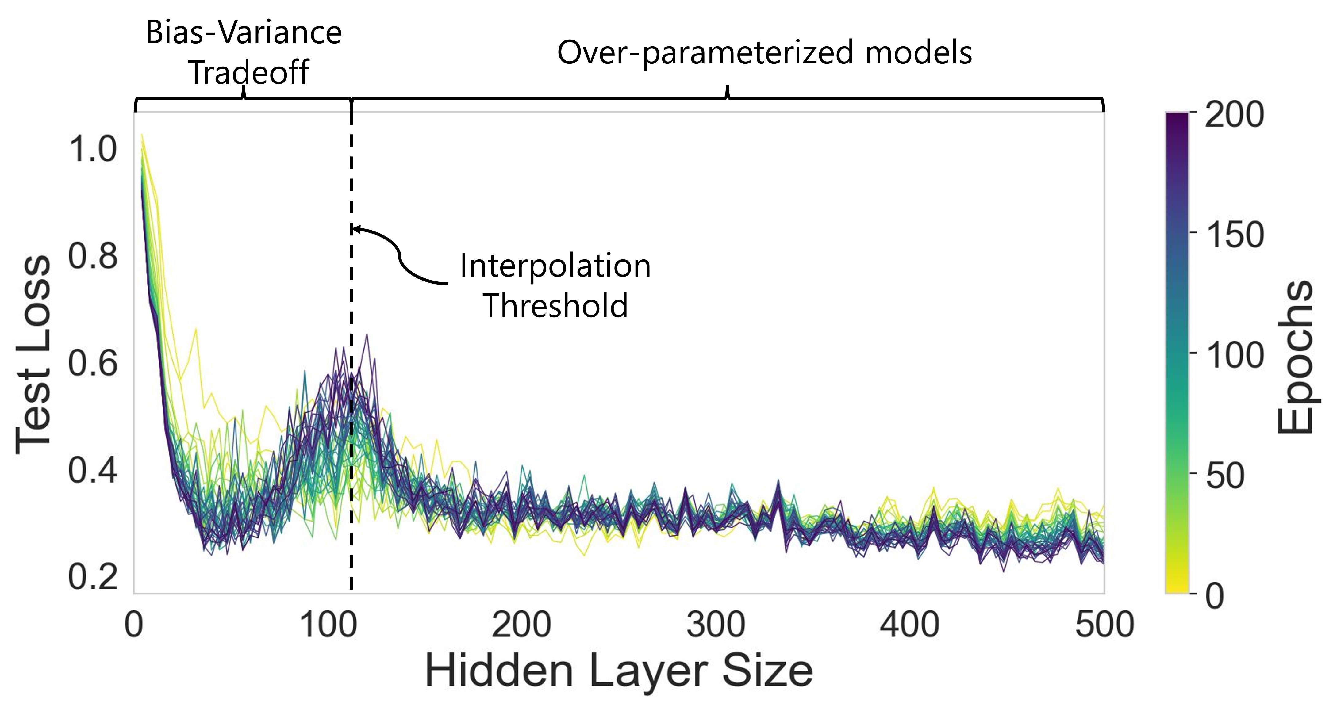
Figure 1: Demonstration of the double descent phenomenon in unsupervised learning. We present the test loss for varying epochs and hidden layer sizes for an under-complete auto-encoder (AE).

2 Related Work

The discovery of double descent for neural networks (NNs) has led to extensive research aimed at understanding the behavior of generalization errors. It has also provided insight into why larger models perform better than smaller or intermediate ones. Most studies have been conducted in a supervised learning setting, as detailed in [9, 10, 11, 12, 13, 14, 15, 16, 20]. Recent studies [10, 21, 22] have introduced label and feature noise and demonstrated that large over-parameterized NNs can "memorize" the noise while still generalizing better than smaller models.

The phenomenon of double descent has not been extensively studied in the context of unsupervised learning, and there are some contradictions in the literature regarding its presence. Principal Component Analysis (PCA) [23] and Principal Component Regression (PCR) [24], which are special types of linear AEs, are widely used unsupervised learning models and can serve as an interesting case study for double descent. The authors in [25] argued that there is no double descent in PCA while [26, 27] show evidence for double descent in PCR and oracle-PCR, respectively. The authors in [28] used a specific subspace data model and argued that there is no sign of model-wise double descent in both linear and non-linear AEs. [29, 30] demonstrate sample-wise double descent for denoising AEs with different Signal-to-Noise Ratios (SNRs). The research in [31] used a self-supervised learning framework for signal processing and found epoch-wise double descent for different levels of noise.

Our analysis of double descent differs from previously published studies in three significant ways. Firstly, when trained on noisy data, we demonstrate that standard under-complete AEs experience double and even triple descent at the model-wise, sample-wise, and epoch-wise levels. We have also partitioned the model’s size into bottleneck and other hidden layer dimensions to understand the phenomenon better. Secondly, we show that the noise magnitude and the number of noisy samples affect the double descent curve. Thirdly, we show that double descent also occurs in common realistic contamination settings in unsupervised learning, such as source-to-target domain shift, anomalous data, and additive feature noise. Finally, we demonstrate the implications of multiple descents in unsupervised learning tasks using real-world data, extending beyond reconstruction.

3 Data Model

This section outlines the data and contamination models we used to study double descent.

3.1 Linear Subspace Data

We will start our experiment by utilizing the synthetic dataset from [28] to challenge their assertion that “double descent does not occur in self-supervised settings”. First, we sample $N$ random i.i.d. Gaussian vectors, each of size $d$, representing random features in a latent space, $z_{i}\sim\mathcal{N}(0,I_{d})$. Next, we embed the vectors $\{z_{i}\}_{i=1}^{N}$ into a higher dimensional space of size $n$ by multiplying each $z_{i}$ by $D$ of size $n\times d$, $Dz_{i}$, where $D_{ij}\sim\mathcal{N}(0,1)$. This setting can be thought of as measuring $\{z_{i}\}_{i=1}^{N}$ with a measurement tool $D$, resulting in higher-dimensional data. Our dataset differs from that of [28] in several ways, and we will investigate four scenarios as part of our study:

Sample Noise. We aim to investigate the impact of the number of noisy training samples on the test loss curve. In contrast to [28], which adds noise to all samples, we vary the number of noisy training samples to identify memorization. We do this by introducing a new variable, $p$, representing the probability of a sample being noisy. Thus, $p\cdot 100\%$ represents the percentage of noisy samples in the data. As noise is added, we control the SNR. We define $\theta$ as the factor controlling the SNR between the signal and the noise. Another significant change from [28] is the chosen values of SNR, which can be found in Appendix A, table 1, along with its calculation to derive $\theta$, in Appendix B. This leads to the following equations, which describe our model for sample noise:

$$x_{i}=\begin{cases}\theta Dz_{i}+\epsilon_{i},&\text{with probability }p,\\ \theta Dz_{i},&\text{with probability }1-p,\end{cases}$$

where $\epsilon_{i}\sim\mathcal{N}(0,I_{n})$ is an additive white Gaussian noise (AWGN), representing the noise added to samples with probability $p$. This setting can be likened to using a noisy measurement device. To illustrate this generation we present in Appendix A, Figure 19 a visualization of the data model.

Feature Noise. We further study the impact of the number of noisy training features on the test loss curve. In the scenario of feature noise, each sample $\{\theta Dz_{i}\}_{i=1}^{N}$ is affected by noise in certain features. We denote the probability of a feature being noisy by $p$, controlling each sample’s noisy features. We simulate a scenario where we have $n$ measuring tools, each measuring a feature. To introduce noise, we select the same set of features to be noisy across all samples. This mimics a situation where $\lfloor n\cdot p\rfloor$ of the measuring tools are unreliable or noisy. Since the noise added to each sample is a vector of length $\lfloor n\cdot p\rfloor$, the SNR calculation differs from the case of sample noise and is explained in Appendix B. Appendix A, Figure 19 depicts the data generation for this setting.

Domain Shift. We aim to explore how the test loss curve behaves when there is a domain shift between the train and test data. To achieve this, we partition the vectors in the latent space $\{z_{i}\}_{i=1}^{N}$ into two groups: train and test vectors, denoted as $z_{train}^{i}$ and $z_{test}^{i}$ respectively. Then, the train vectors are projected to higher dimensional space with the matrix $D$, and the test vectors are projected with a different matrix $D^{{}^{\prime\prime}}$, modeling a domain shift. To control the shift, we define $D^{{}^{\prime\prime}}=D+s\cdot D^{{}^{\prime}}$, where $D$ is the matrix multiplying the train vectors and $D_{ij}^{{}^{\prime}}\sim\mathcal{N}(0,1)$ is a new random matrix added to $D$ to cause perturbations at each entry of $D$. The parameter $s$ controls the shift between $D$ and $D^{{}^{\prime\prime}}$. As a result, for $s\neq 0$, a domain shift is present between the train and test datasets, and we get

$$x_{i}=\begin{cases}Dz_{train}^{i},&\text{if }train,\\ D^{{}^{\prime\prime}}z_{test}^{i},&\text{if }test.\end{cases}$$

It is important to note that because $D$ and $D^{\prime}$ are i.i.d., $D^{\prime\prime}$ follows a normal distribution $\mathcal{N}(0,(1+s^{2})I)$. To obtain the same norm in the test data, we divide $D^{\prime\prime}$ by $\sqrt{1+s^{2}}$. This scenario is similar to the case where two different measuring instruments (i.e., $D,D^{{}^{\prime\prime}}$) are measuring the same phenomenon. This data model is illustrated in Appendix A, Figure 20, and the definition of the SNR is detailed in Appendix B.

Anomalies. We conduct an experiment to investigate the impact of anomalies in the training set on the test loss curve. To represent clean samples, we utilize $\{\theta Dz_{i}\}_{i=1}^{N}$. For generating anomalies, we sample from a normal distribution $\mathcal{N}(0,I_{n})$. We introduce a metric termed signal-to-anomaly-ratio (SAR), which regulates the magnitude ratio between the clean and anomaly samples through the parameter $\theta$. Subsequently, we substitute $p\cdot 100\%$ of the normal samples with anomalies. This generation is illustrated in Appendix A, Figure 21.

We generate 5000 samples for training and 10000 for testing across all of these scenarios.

3.2 Single-Cell RNA Data

We utilized single-cell RNA sequencing data from [32] to illustrate our findings using real-world data. The data exhibits diverse domain shifts across different laboratory environments and measurement technologies. This dataset is crucial for assessing the impact of domain shifts on the test loss curve. Since this data is from a real-world setting, we are unable to control the shifts between the training (source) and testing (target) datasets, as explained in Section 3.1. We focused on dataset number 4, which includes 5 distinct domains named ’Baron’, ’Mutaro,’ ’Segerstolpe,’ ’Wang,’ and ’Xin’ and 15 different cell types. Each cell (sample) contains over 15000 genes (features). To facilitate the training of deep models while preserving the domain shift, we have retained the top 1000 prominent features. We utilize the ’Baron’ domain for both sample and feature noise and domain shift scenarios due to its largest sample size (8569). 5000 samples are allocated for training and the reserved 3569 samples are for testing. Additive white Gaussian noise (AWGN) is added to specific training samples and features, as described in 3.1. The calculations of the SNR for both sample and feature noise cases are provided in Section B. As for the domain shift scenario, the target batches are ’Mutaro’ (2122 samples), ’Segerstople’ (2127 samples), ’Wang’ (457 samples), and ’Xin’ (1492 samples).

4 Results

All the experiments are conducted using multi-layer perceptron under-complete AEs utilizing at least 5 different random seeds. Complete implementation details can be found in Appendix A. All models are trained using contaminated datasets and tested on clean data. Consequently, the test loss serves as an indicator of whether the model has learned the noisy data (high test loss) or the signal (low test loss). This concept is akin to label noise in supervised learning, as discussed in [10]. The train loss figures corresponding to all test losses depicted in this section are provided in Appendix C.

4.1 Model-Wise Double Descent

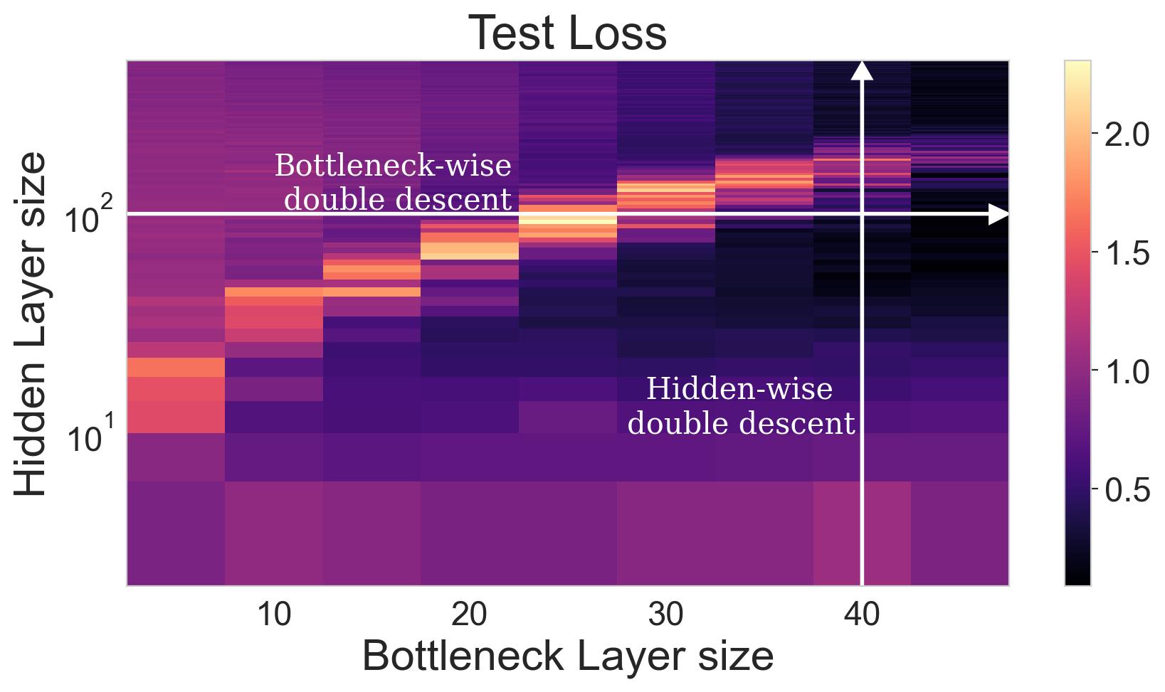
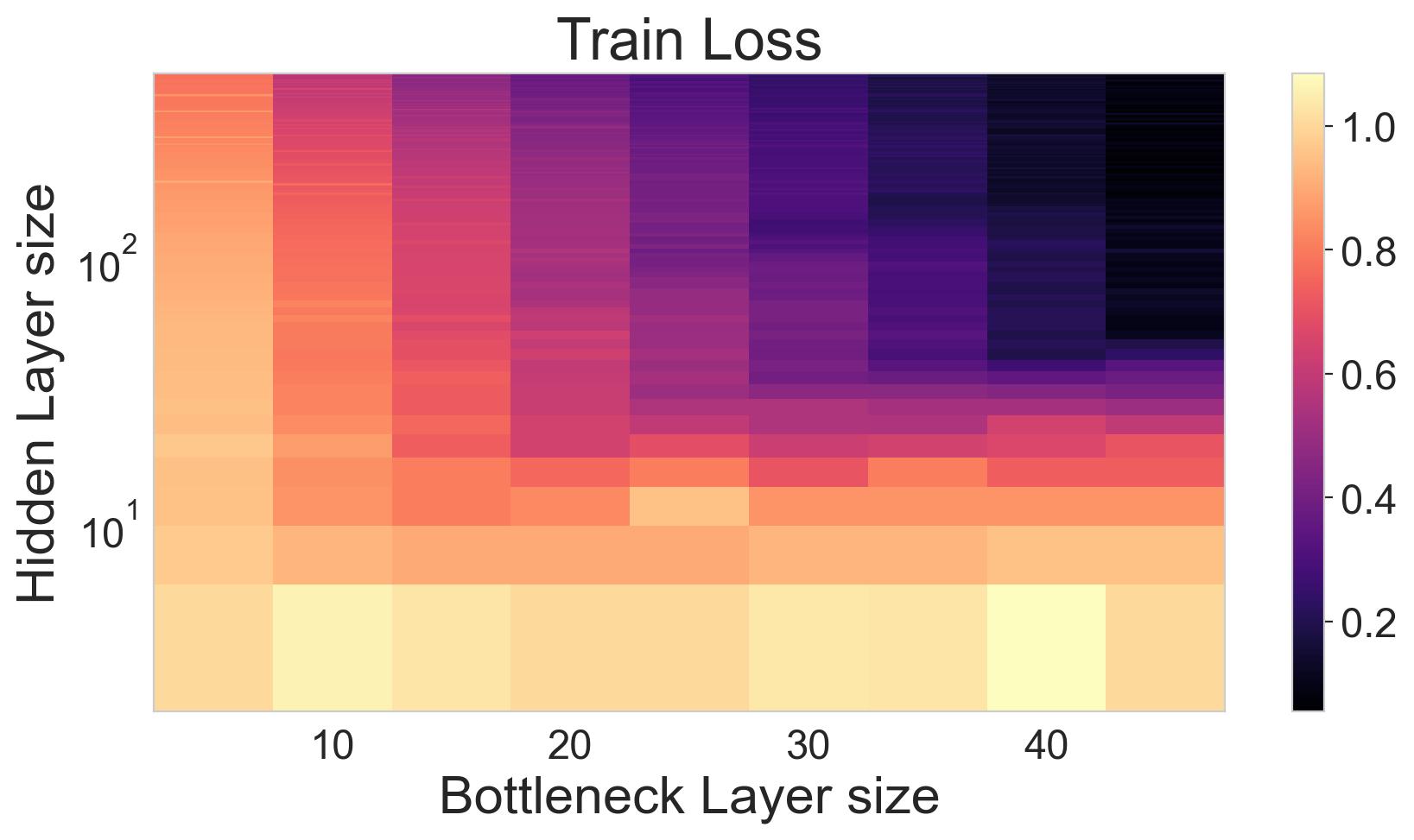
Figure 2: Test and train losses as a function of bottleneck and hidden layer sizes. While the training loss decreases for larger models, the test loss demonstrates clear double descent when varying the bottleneck or hidden layer size. The AEs were trained on the linear subspace model with sample noise = 90% and SNR = -15 [dB] (see details in Section 3.1).

This section analyzes the test loss with increasing model sizes. For AEs, we break down the well-known "double descent" phenomenon into two interconnected variations: "hidden-wise" and "bottleneck-wise" double descent. We show how both contribute to the double descent behavior in the test loss. We also study the influence of several contaminations described in Section 3. We conclude that the interpolation threshold location and value can be manipulated by these factors.

In Figure 2, we provide visual evidence of the bottleneck-wise and hidden-wise double descent. This not only helps to distinguish between various model sizes but also underscores the significance of our different architectural choices. As can be seen the training loss consistently decreases as the dimensions of the model increase. In contrast, both the bottleneck and hidden layers exhibit the characteristic double descent curve, as seen in the decrease in test loss, followed by an increase and then another decline. This clear demonstration of double descent corroborates that AEs trained on highly contaminated data can exhibit double descent.

Sample noise. Interestingly, Figure 3(a) shows that the height of the test loss increases and the interpolation threshold peak location shifts towards larger models as the level of sample noise increases. This can be clarified by the observation that increased noise adversely affects model learning. Moreover, we need a bigger model to overfit the noisy samples. For sample noise ranging from 10% to 20%, the absence of double descent can be attributed to an insufficient number of noisy samples in the training data. In Figure 3(b), we demonstrate triple descent using single-cell RNA data, where we notice a similar behavior for the test loss, and specifically for each of the two peaks. Furthermore, all instances of sample noise exhibiting double and triple descent present a lower test loss in the second or third descent in comparison to the first, excluding 80% and 90% in 3(a).

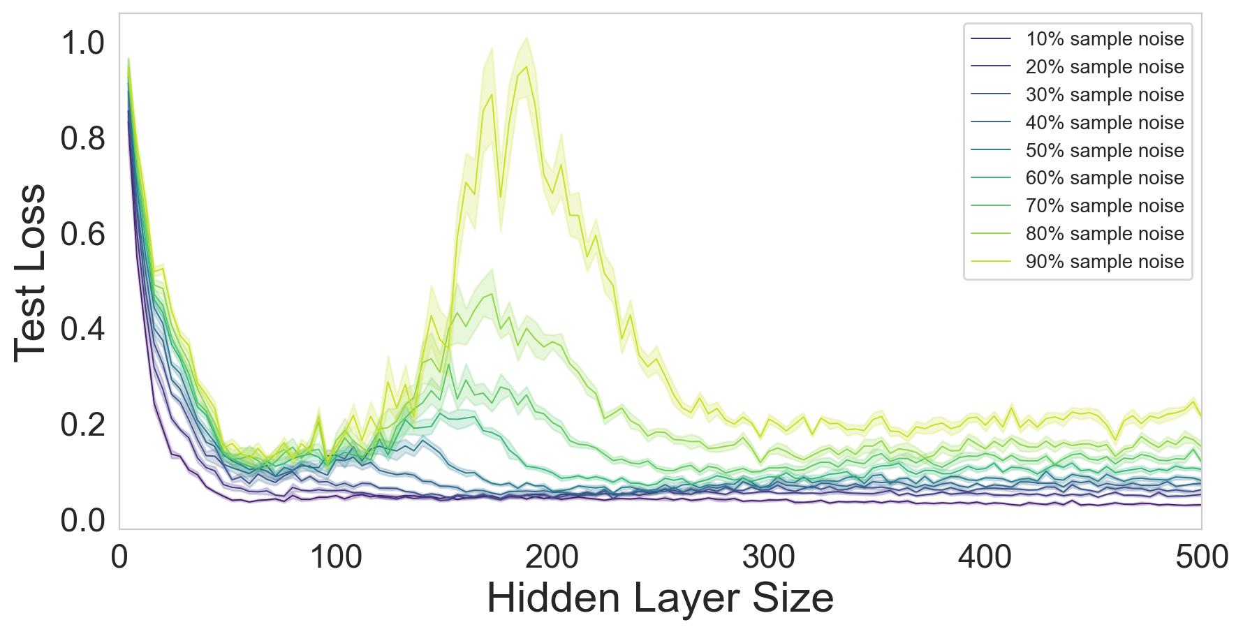
(a) Linear subspace data exhibits model-wise double descent with SNR = -15 [dB].

(b) Single-cell RNA data exhibits model-wise triple descent with SNR = -17 [dB].

Figure 3: Test loss exhibits model-wise double and triple descents for the case of varying sample noise. Train losses are depicted Appendix C, Figure 23.

Feature noise. Feature noise adds complexity since each sample contains noise in some of its features. As a result, the model never encounters samples with entirely clean features, making it unable to isolate and focus on clean data. Consequently, the model experiences difficulty in learning the correct data structure. Surprisingly, increasing feature noise actually leads to a decrease in the test loss for the single-cell RNA dataset (Figure 4(b)) and an increase for the case of linear subspace data. Moreover, the peak shifts left as the number of noisy features rise in Figure 4(a).

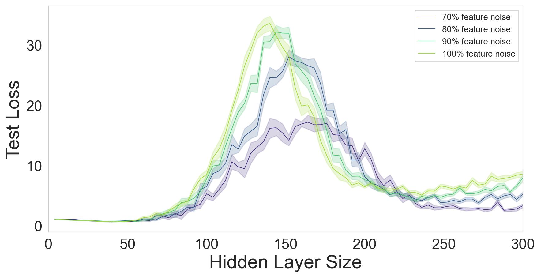
(a) Double descent for the linear subspace data trained with SNR = -13 [dB]. Beyond a hidden layer of size 300, the test loss exhibits a rise.

(b) Non-monotonic behavior for the Single-cell RNA data trained with SNR = -12 [dB]. Beyond a hidden layer size of 2000, the test loss continues to decrease, while the train loss increases.

Figure 4: Test loss exhibits model-wise double descent and non-monotonic behaviors for the case of varying feature noise. Train losses are illustrated in Appendix C, Figure 24.

SNR. We observed that the SNR plays a crucial role in the test loss, which in turn affects the height of the peak. A higher SNR value reduces the impact of noise, allowing the model to learn the underlying signal from the training set, resulting in a lower test loss. Conversely, a lower SNR value amplifies the influence of noise, causing the model to minimize the training loss by memorizing the noise rather than learning the signal. This leads to inferior results in the test loss. Figures 5 and 6 demonstrate this for the scenarios of sample and feature noise respectively.

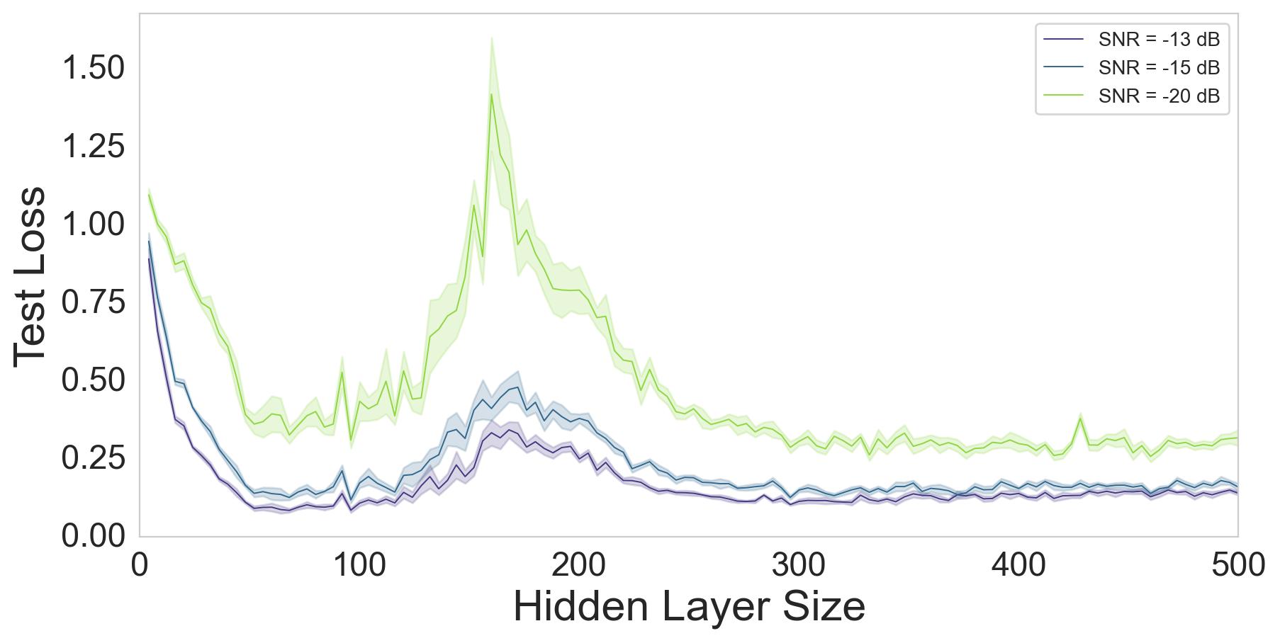
(a) Linear subspace data. Sample noise = 80%.

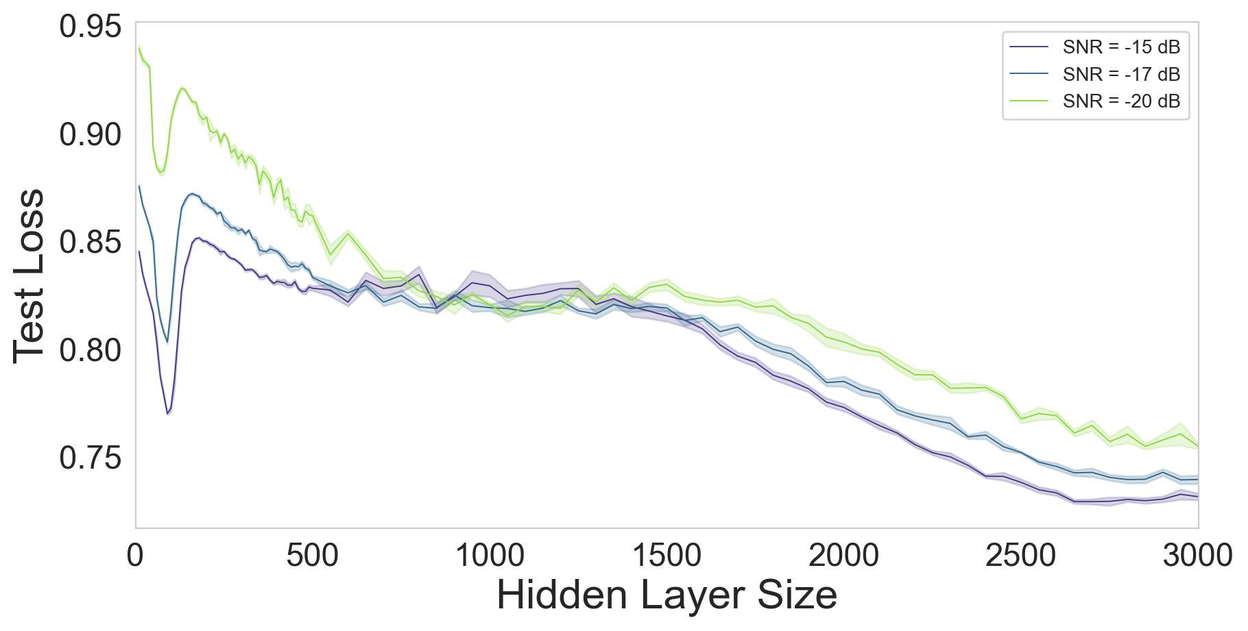
(b) Single-cell RNA data. Sample noise = 40%.

Figure 5: The effect of SNR for the case of noisy samples on the test loss curve. Train losses are illustrated in Appendix C, Figure 25.

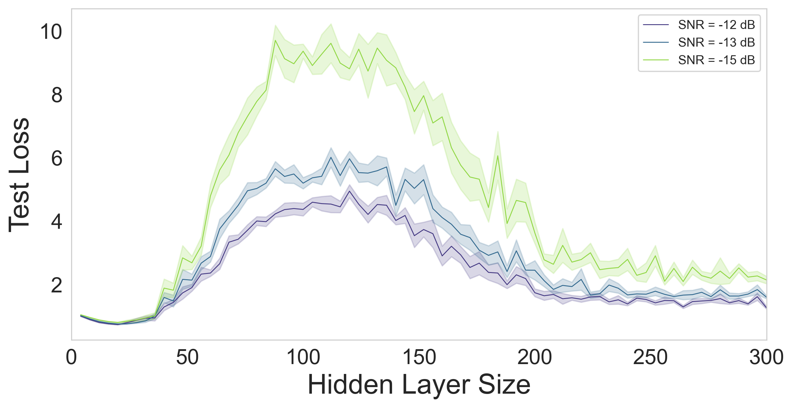
(a) Linear subspace data with 40% noisy features. Beyond hidden layer of size 300, the test loss rises.

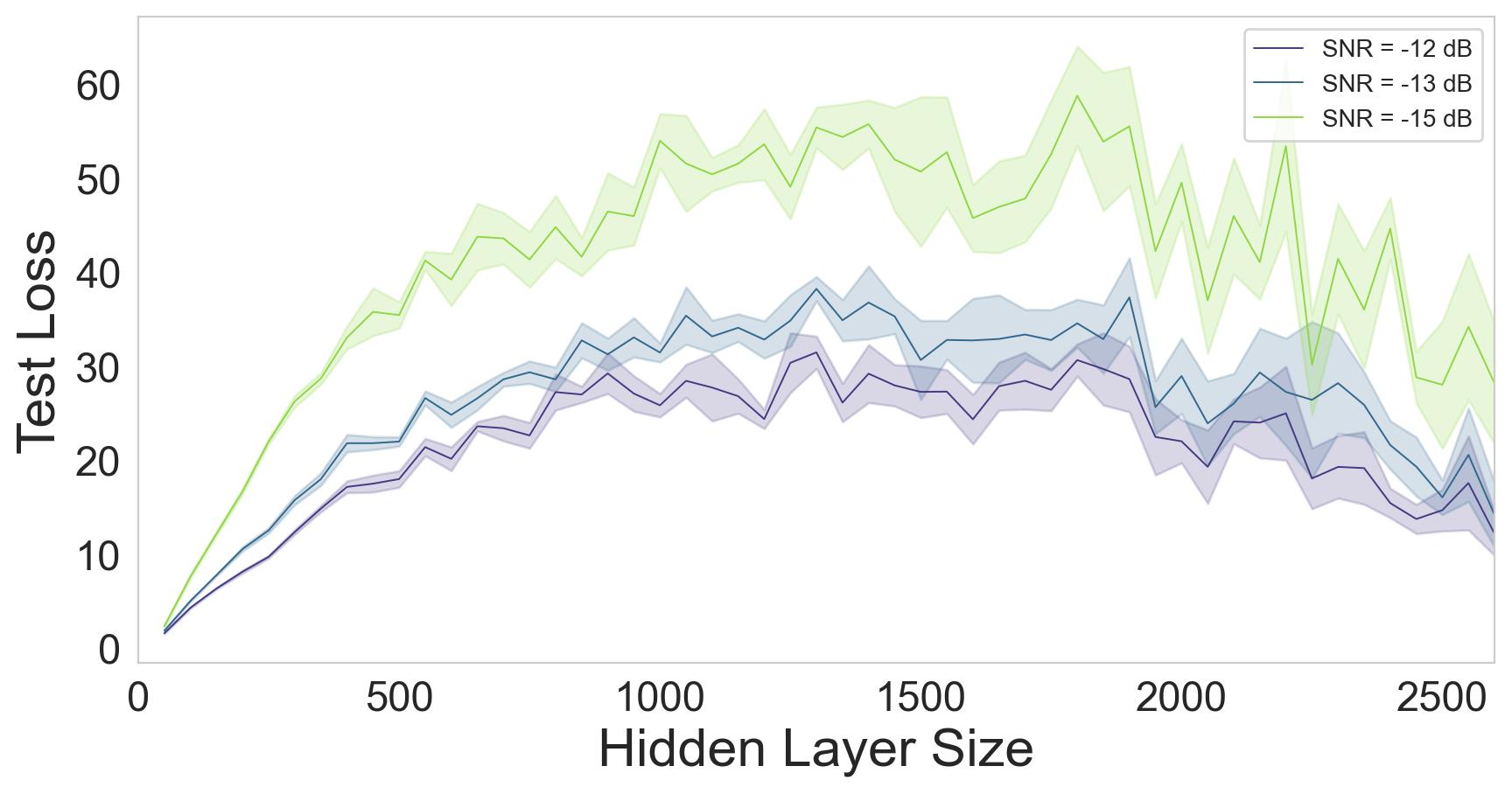
(b) Single-cell RNA data with 10% noisy features. Beyond a hidden layer size of 2600, the test loss continues to decrease, and the train loss increases.

Figure 6: The effect of SNR for the case of noisy features on the test loss curve. Train losses are depicted in Appendix C, Figure 26.

Domain shift. We now study the existence of double descent when the distribution of the training (source) data, $D_{s}=\{X_{s},p(x_{s})\}$, differs from that of the testing (target) data, $D_{t}=\{X_{t},p(x_{t})\}$. We investigate the impact of the model size on learning shared representations for both source and target datasets and reducing the shift between them. By training the model on the source data and testing it on different targets, we unveil non-monotonic behavior and double and triple descent curves for synthetic and real datasets discussed in Sections 3.1 and 3.2, respectively. Furthermore, we observe instances where over-parameterized models result in lower test loss, leading to improved target data reconstruction as depicted in Figure 7. Additionally, we notice that the test loss rises as the shift is more dominant. Section 5.1 presents double and triple descent for real-world data and further insights about the connection of model size and domain adaptation.

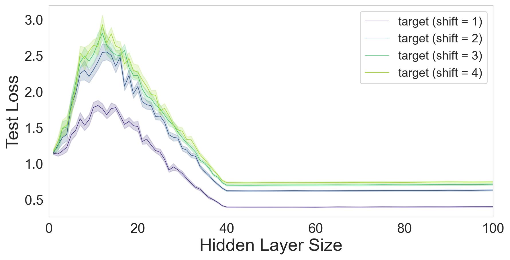
Figure 7: Linear subspace data exhibits model-wise non-monotonic behavior for varying domain shifts. Appendix C, Figure 27 shows the train loss behavior.

Anomaly detection. We also identify double descent occurring when anomalies, deviating from the expected behavior of the data are introduced into the training set. We use the anomaly dataset mentioned in 3.1 and study the test loss curves by varying the amounts of anomalous training samples. We then evaluate the anomaly detection capabilities using the receiver operating characteristic area under the curve (ROC-AUC). This metric employs the reconstruction error score to measure the model’s ability to distinguish between the clean and anomalous data. Anomalies are identified as data points with scores surpassing a defined threshold. A higher ROC-AUC value signifies superior performance. As demonstrated in the interpolation regime depicted in Figure 8(a), interpolating models show higher test loss of the clean samples, complicating the differentiation between clean and anomaly data.

Scaling up the model size, results in a secondary descent in the test loss of the clean data, particularly evident under conditions of low SAR and a high number of anomalies. This secondary descent facilitates the model’s ability to differentiate between clean and anomalous data, resulting in performance comparable to that of smaller models in terms of ROC-AUC, while learning meaningful embedding for both clean data and outliers, resulting in lower test losses. Figure 8(b) demonstrates the absence of double descent due to the high SAR. However, similar to Figure 8(a), intermediate models exhibit poorer ROC-AUC performance compared to small and over-parameterized models. We also present more insights on anomaly detection when utilizing real-world data in Section 5.2.

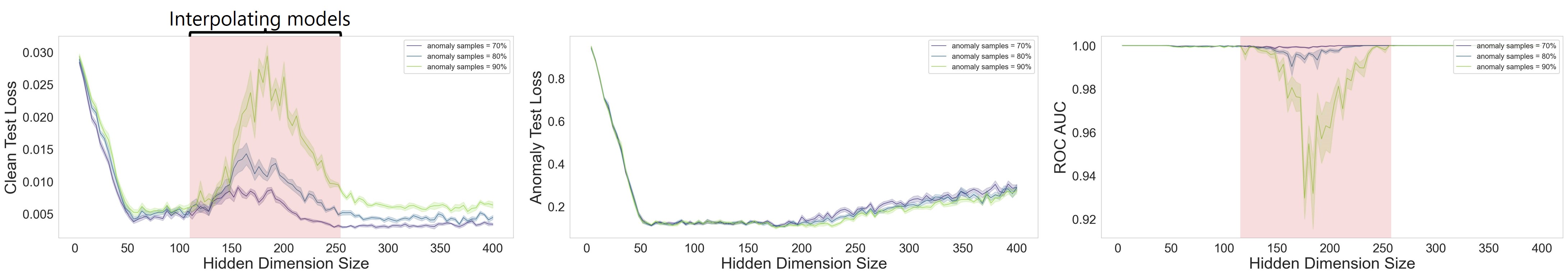
(a) Synthetic anomaly data with SAR = -15 [dB].

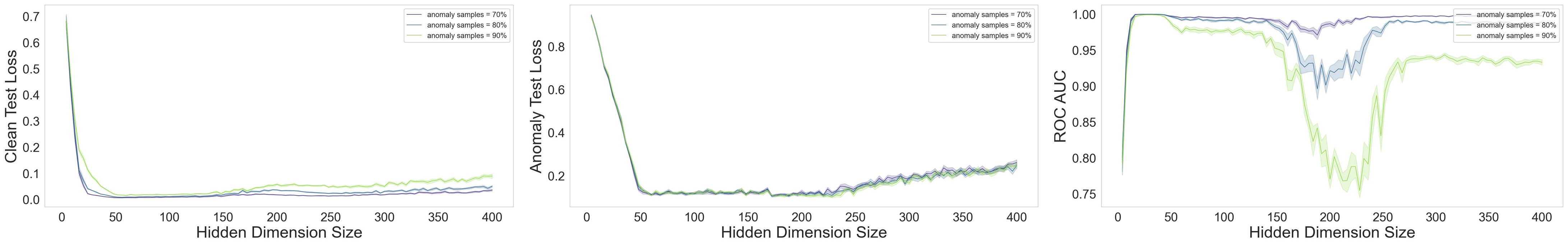
(b) Synthetic anomaly data with SAR = 0 [dB].

Figure 8: Left: test loss of the clean samples. A double descent pattern emerges for low SARs (mentioned in 3.1) and high anomaly presence in the training data. Middle: test loss of the anomaly data. Right: Non-monotonic behavior of the ROC-AUC.

4.2 Epoch-Wise Double Descent

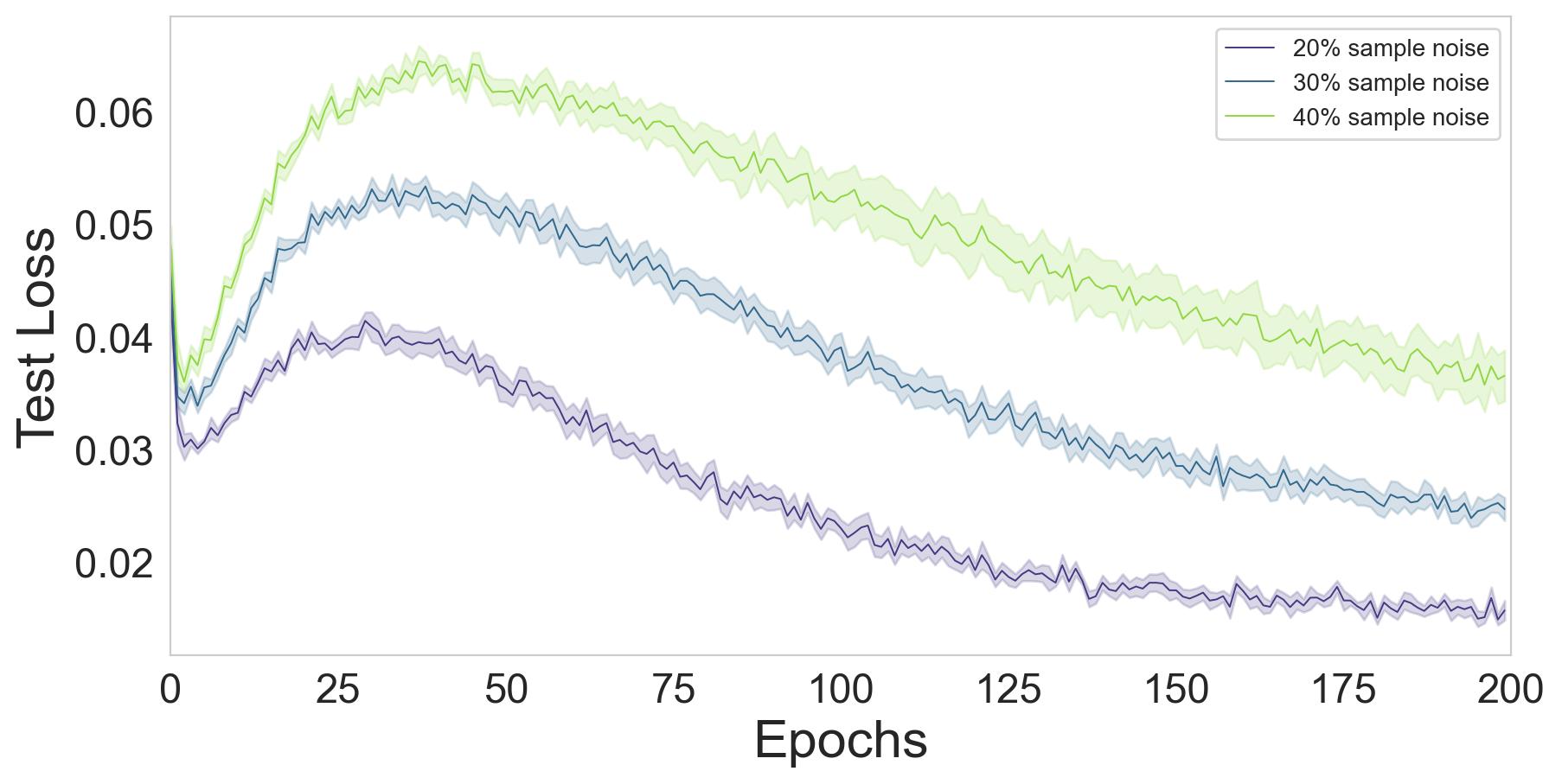
(a) Linear subspace data with SNR = -2 [dB].

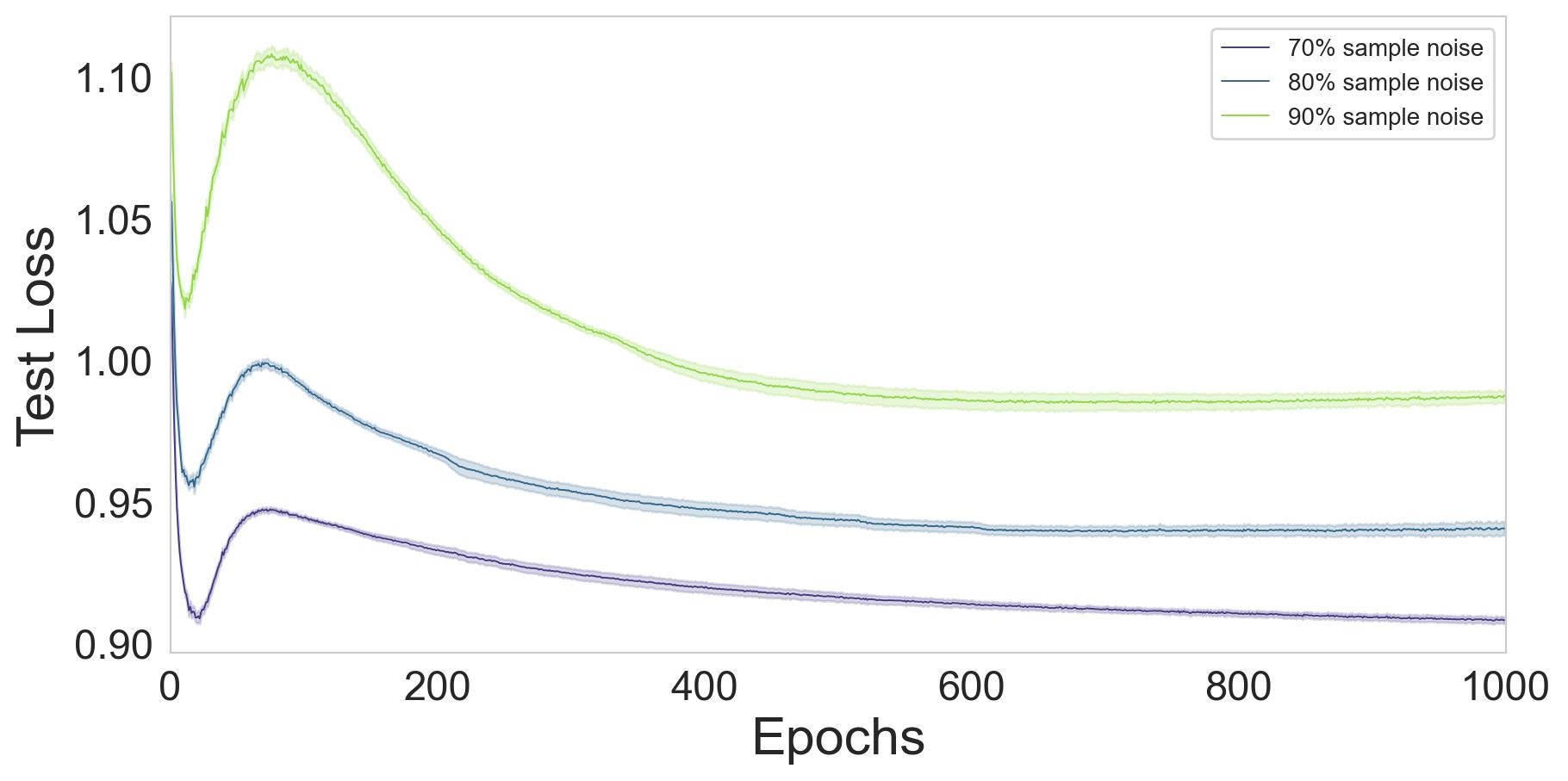
(b) Single-cell RNA data with SNR = -17 [dB].

Figure 9: Epoch-wise double descent influenced by the number of noisy samples. Train losses are depicted in Appendix C, Figure 28.

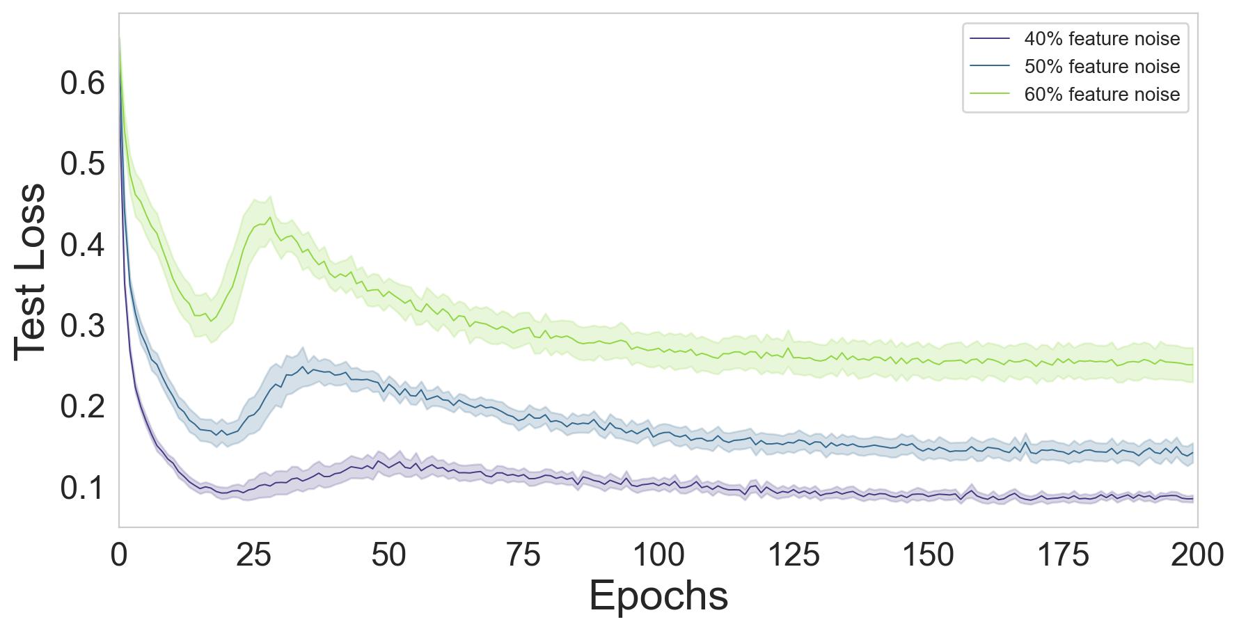
(a) Linear subspace data with SNR = -12 [dB].

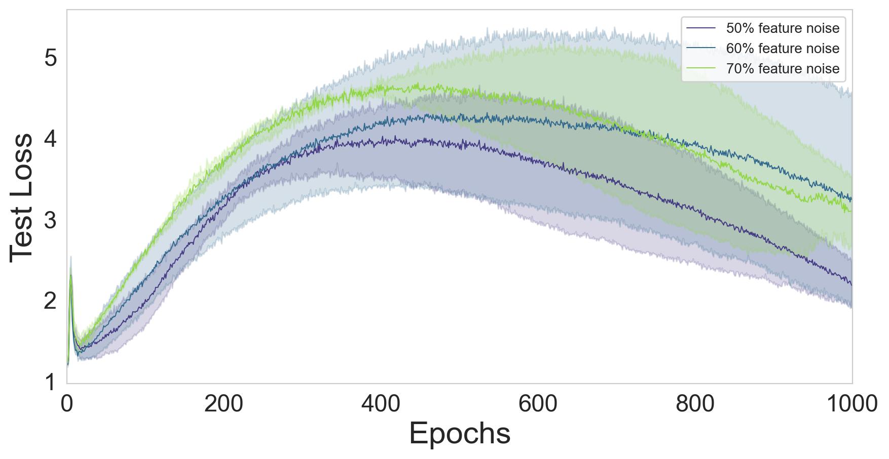
(b) Single-cell RNA data with SNR = -12 [dB].

Figure 10: Epoch-wise double descent influenced by the number of noisy features. Train losses are illustrated in Appendix C, Figure 29.

In this section, we study the concept of double descent with respect to the number of epochs. This work is the first unsupervised investigation of its kind, building upon similar research conducted by [10] for supervised learning. We begin by analyzing the impact of the number of noisy samples and features in the train set on the test loss.

Figures 9 and 10 show the results for both data models respectively. As the portion of noisy samples or features increases, the test loss becomes higher since the model tends to prioritize overfitting the noise rather than learning the signal.

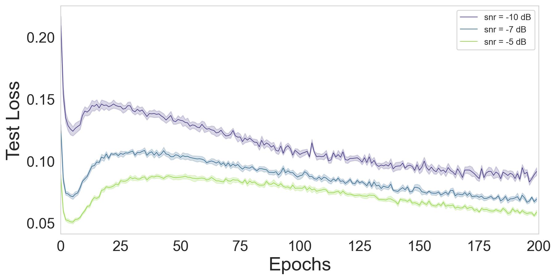
(a) Linear subspace data. Sample noise = 40%.

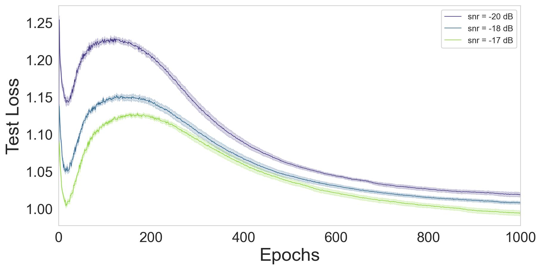
(b) Single-cell RNA data. Sample noise = 90%.

Figure 11: Epoch-wise double descent for the case of sample noise influenced by the SNR. Train losses are exhibited in Appendix C, Figure 30.

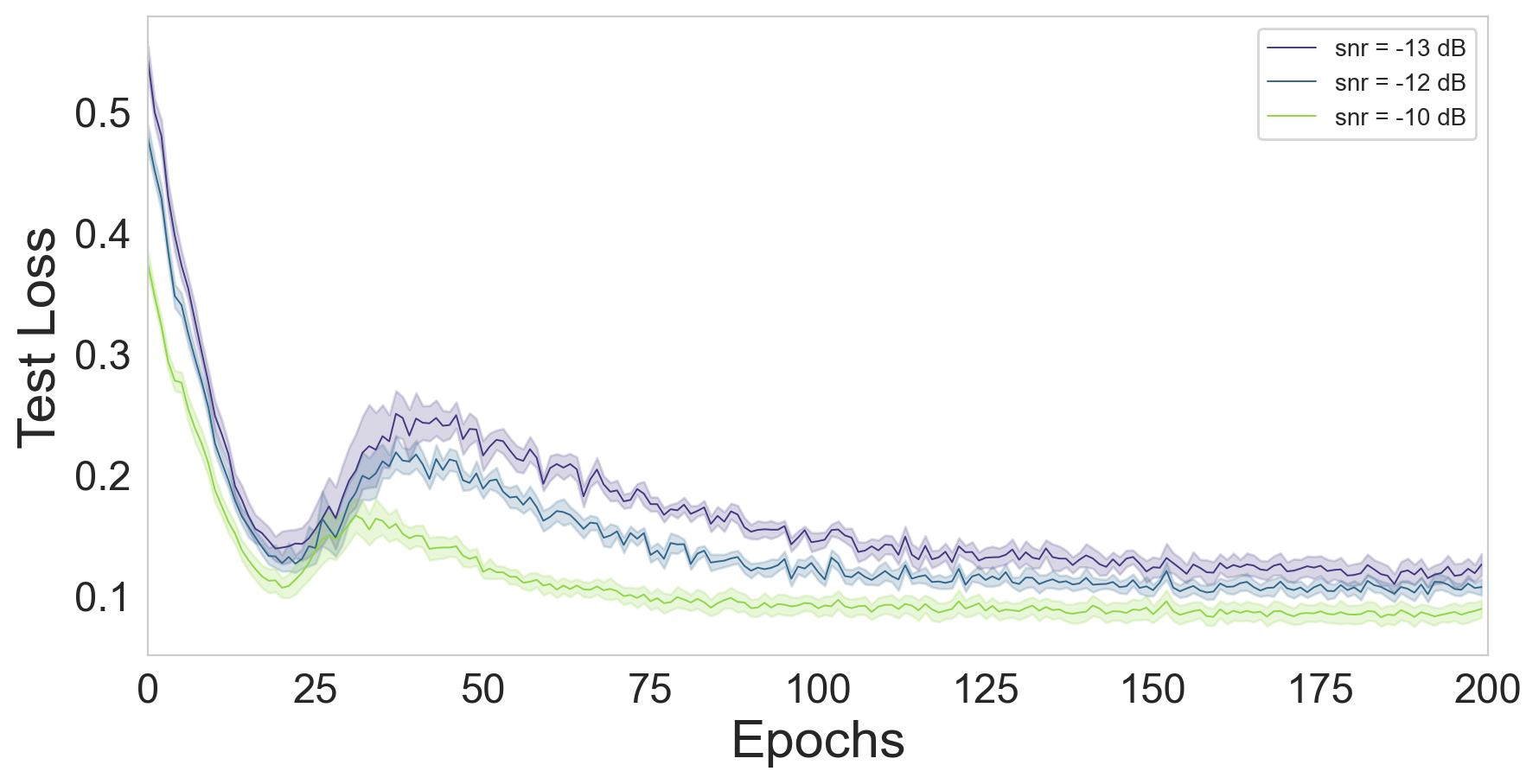
(a) Linear subspace data. Feature noise = 80%.

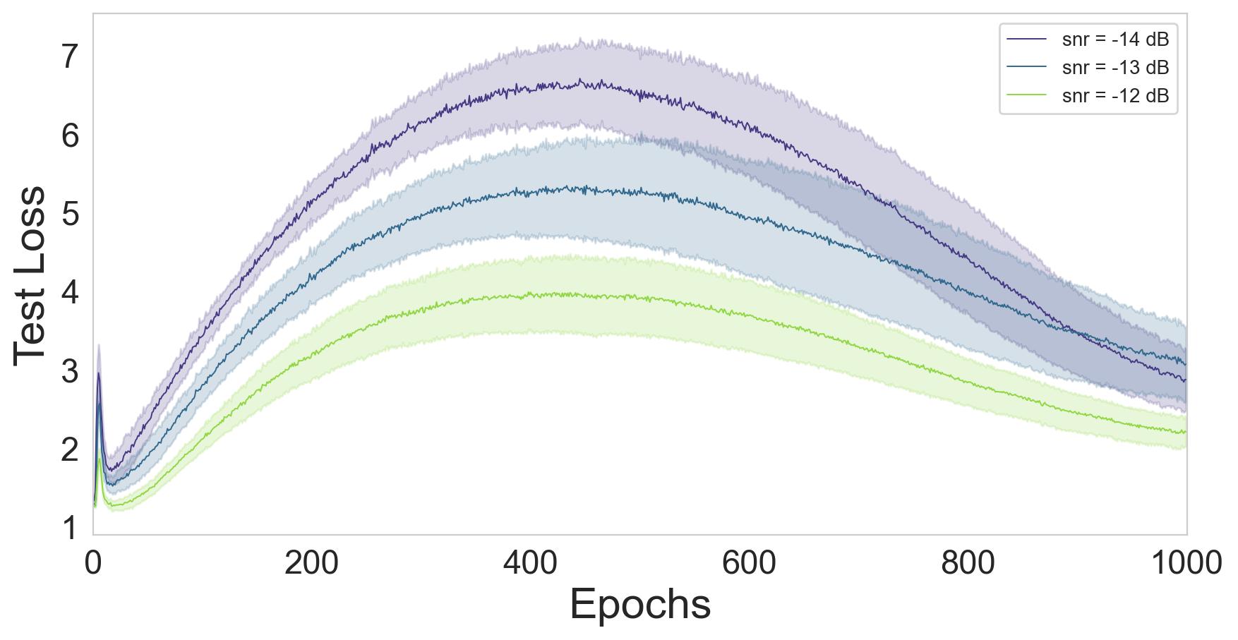
(b) Single-cell RNA data. Feature noise = 50%.

Figure 12: Epoch-wise double descent for the case of feature noise influenced by the SNR. Train losses are illustrated in Appendix C, Figure 31.

We have conducted further research on epoch-wise double descent, which has led us to discover a connection between the SNR and the height of the test loss. As the SNR decreases, the noise becomes more dominant, resulting in an increase in the test loss. This is illustrated in Figures 11 and 12 for the cases of sample and feature noise respectively.

Epoch-wise double descent is also present when there is a domain shift between the train and test sets, as illustrated in Figure 13. 13(a) shows that the stronger the shift, the higher the test loss.

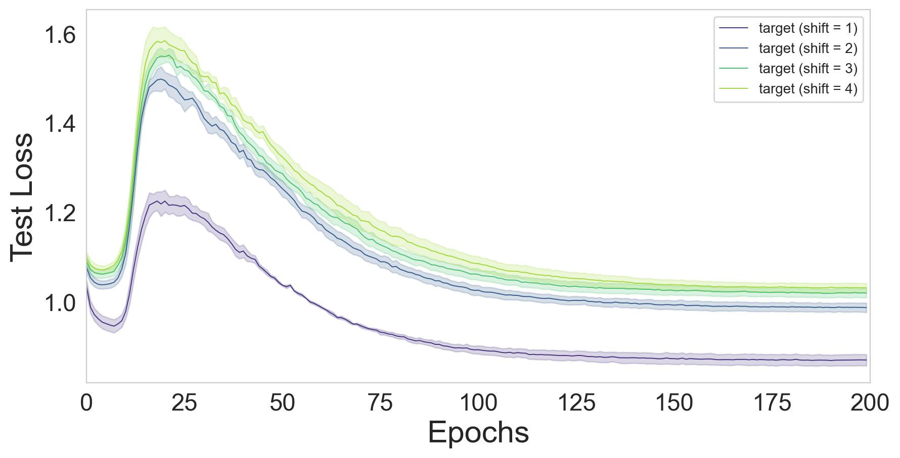
(a) Linear subspace data with 5% noisy samples and SNR = 20 [dB].

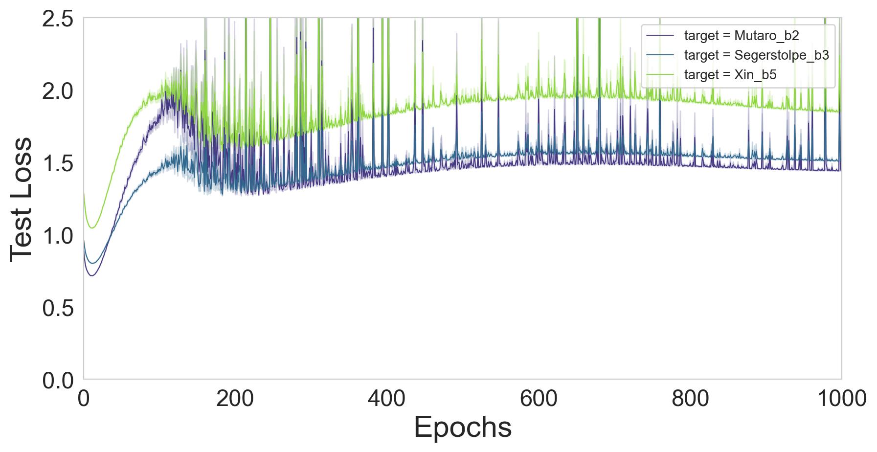
(b) Single-cell RNA data. The ’Wang’ batch (Appendix A) was excluded due to noisy results.

Figure 13: Epoch-wise double descent influenced by the amount of domain shift. Left: we introduce some noise to emphasize the double descent curve. Appendix C, Figure 32 shows the train losses.

4.3 Sample-Wise Double Descent

In this section, we study the impact of changing the number of training samples while keeping the model size constant. The complexity of a model and the number of samples it is trained on, both play a crucial role in determining whether the model is over or under-parameterized. When the sample size is small, the model is considered over-parameterized. However, as the sample size increases, the model enters the under-parameterized regime. This causes the interpolation threshold to shift to the right, as shown in Figure 14 which displays model-wise double descent for different amounts of training data. However, this adjustment can sometimes result in a model that performs worse than a model trained on a smaller set of training samples. A similar phenomenon was demonstrated in [10] in the supervised setting.

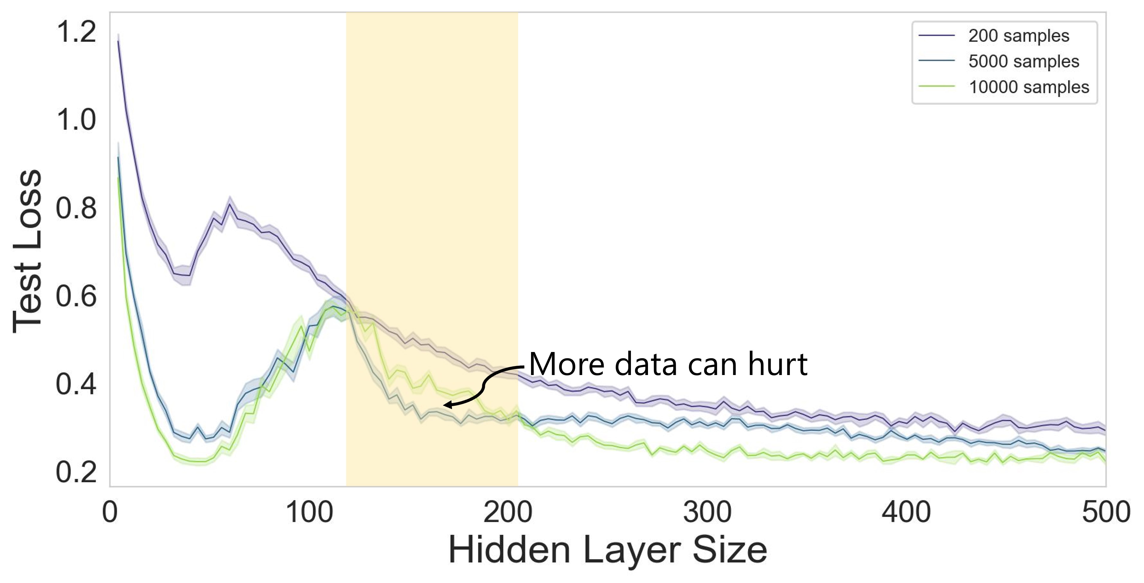
Figure 14: Model-wise double descent for the linear subspace data with different number of training samples. In the yellow interval, models trained with 10000 samples exhibit inferior performance compared to those trained with 5000 samples. Sample noise = 70% and SNR = -15 [dB]. Results for the train losses are exhibited in Appendix C, Figure 33.

We also investigate how gradually increasing the number of training samples affects the test loss curve. Remarkably, we identify a non-monotonic trend in the test loss curve at Figures 15(b), 15(c), 15(d), 15(e), which sometimes results in double descent as noticed in 15(a). The emergence of non-monotonic behavior is defined by a phase where an increased number of samples negatively impacts performance, resulting in higher test loss. Figure 15 showcases only the results from the linear subspace dataset due to the insufficient amount of samples in the single-cell RNA dataset. The impact of the number of noisy samples and features, the SNR, and the domain shift on the test loss is consistent with the analyses conducted in Sections 4.1 and 4.2.

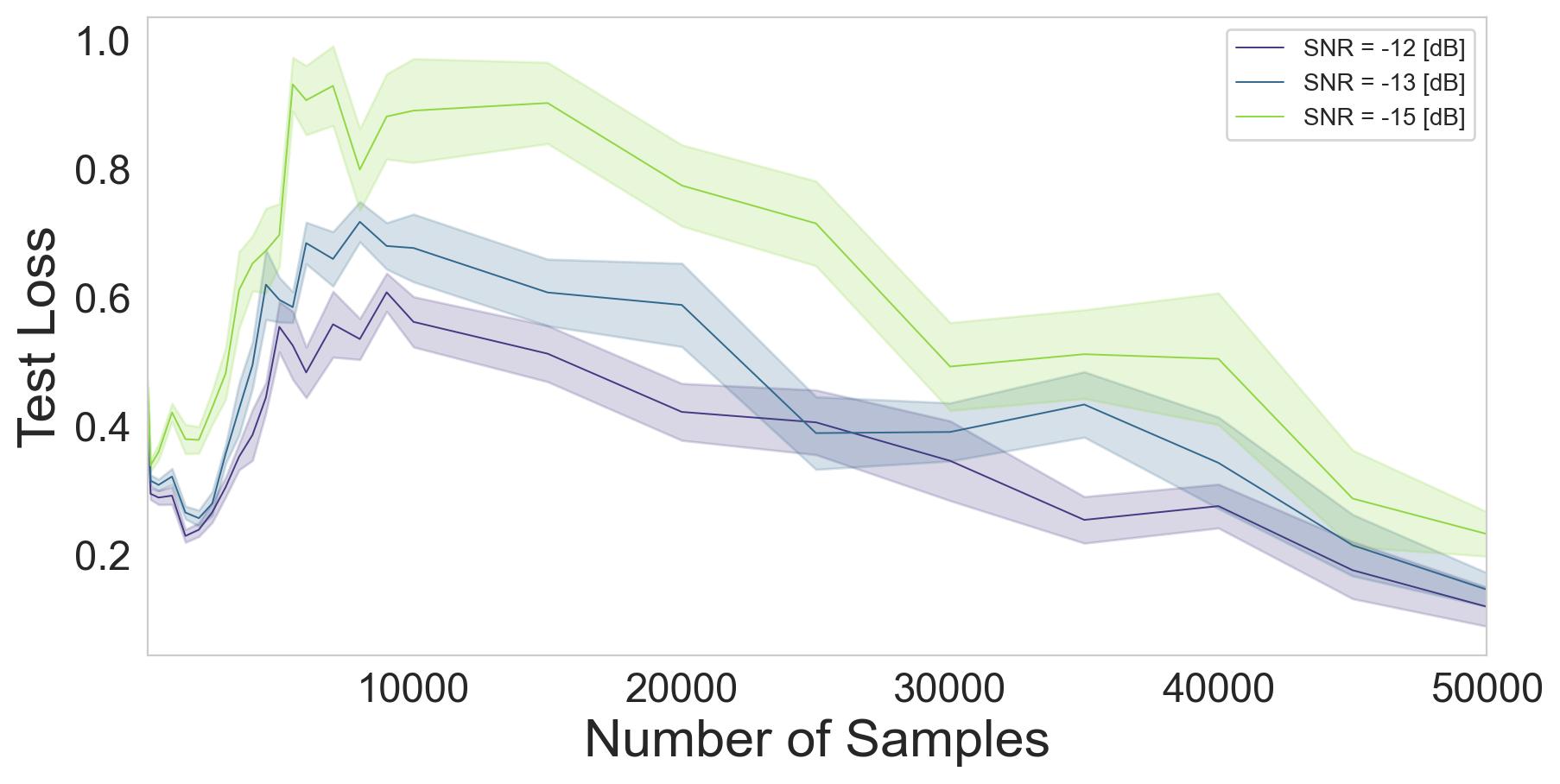
(a) sample noise = 90%.

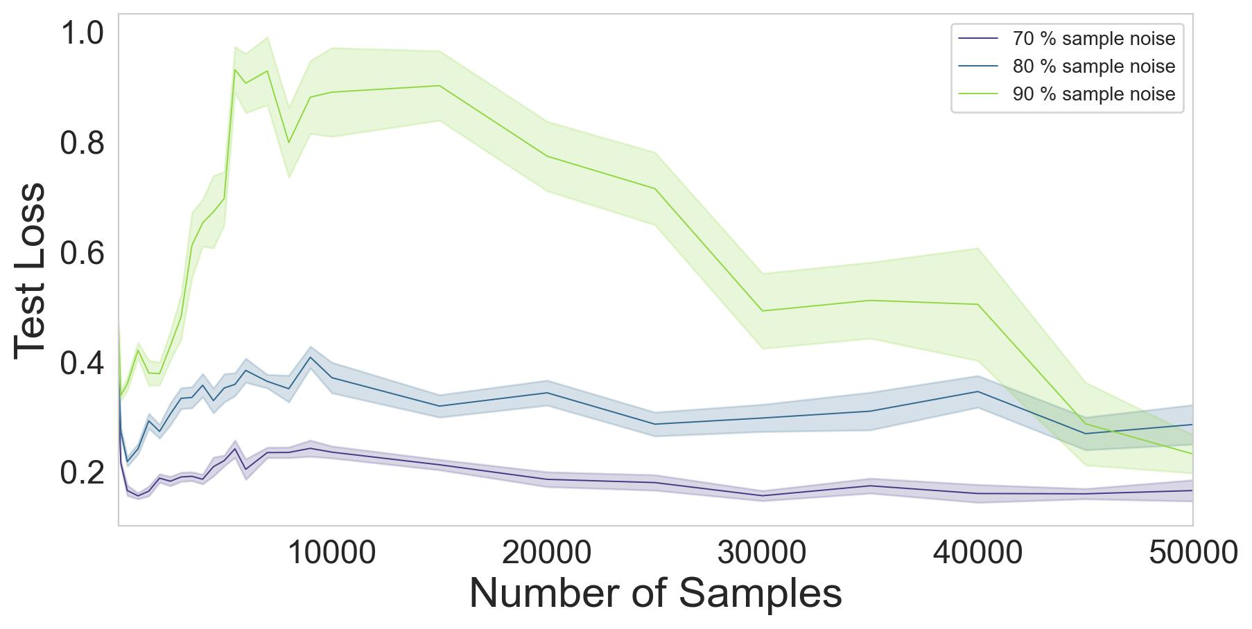
(b) Sample noise scenario. SNR = -15 [dB].

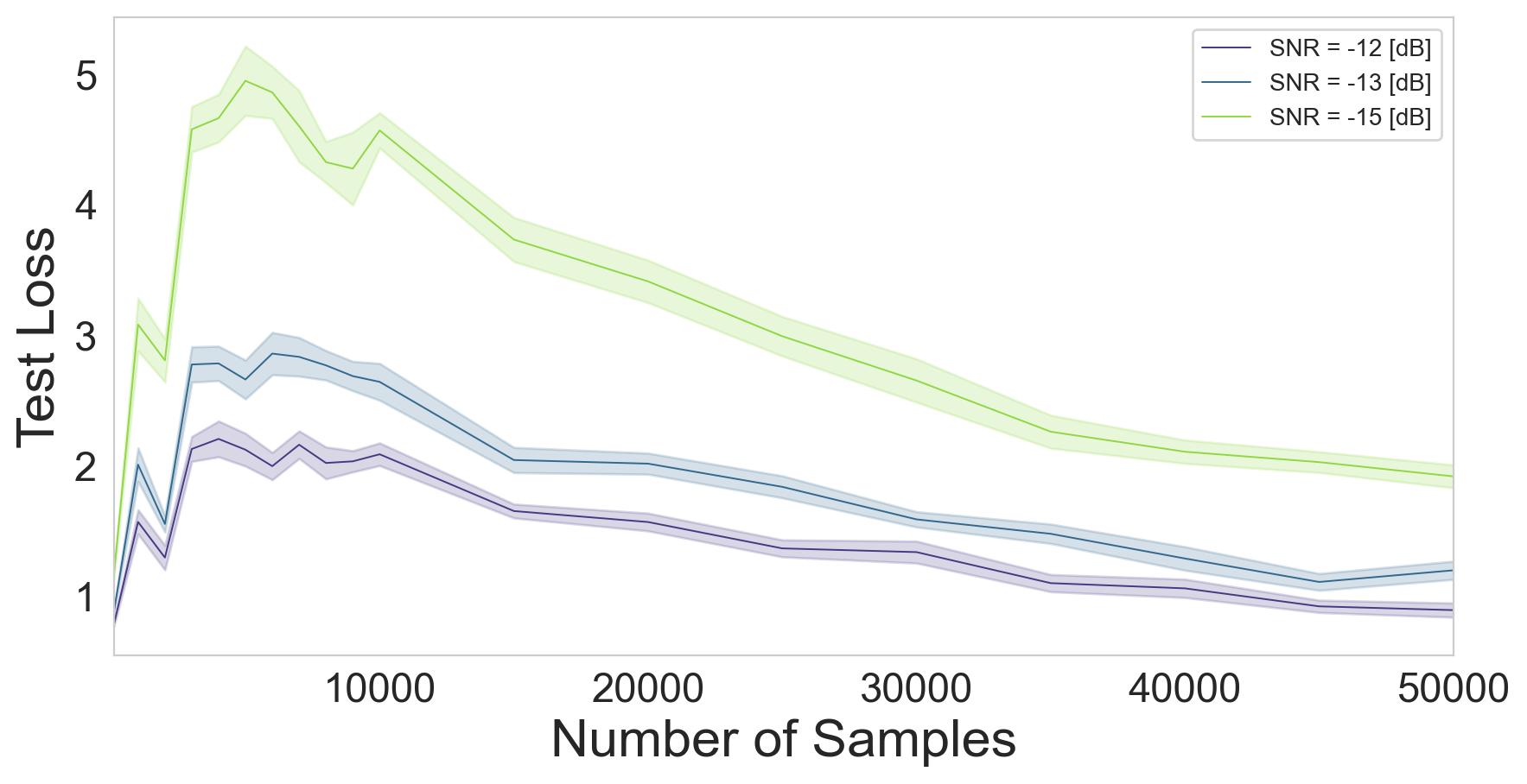
(c) Feature noise = 90 %.

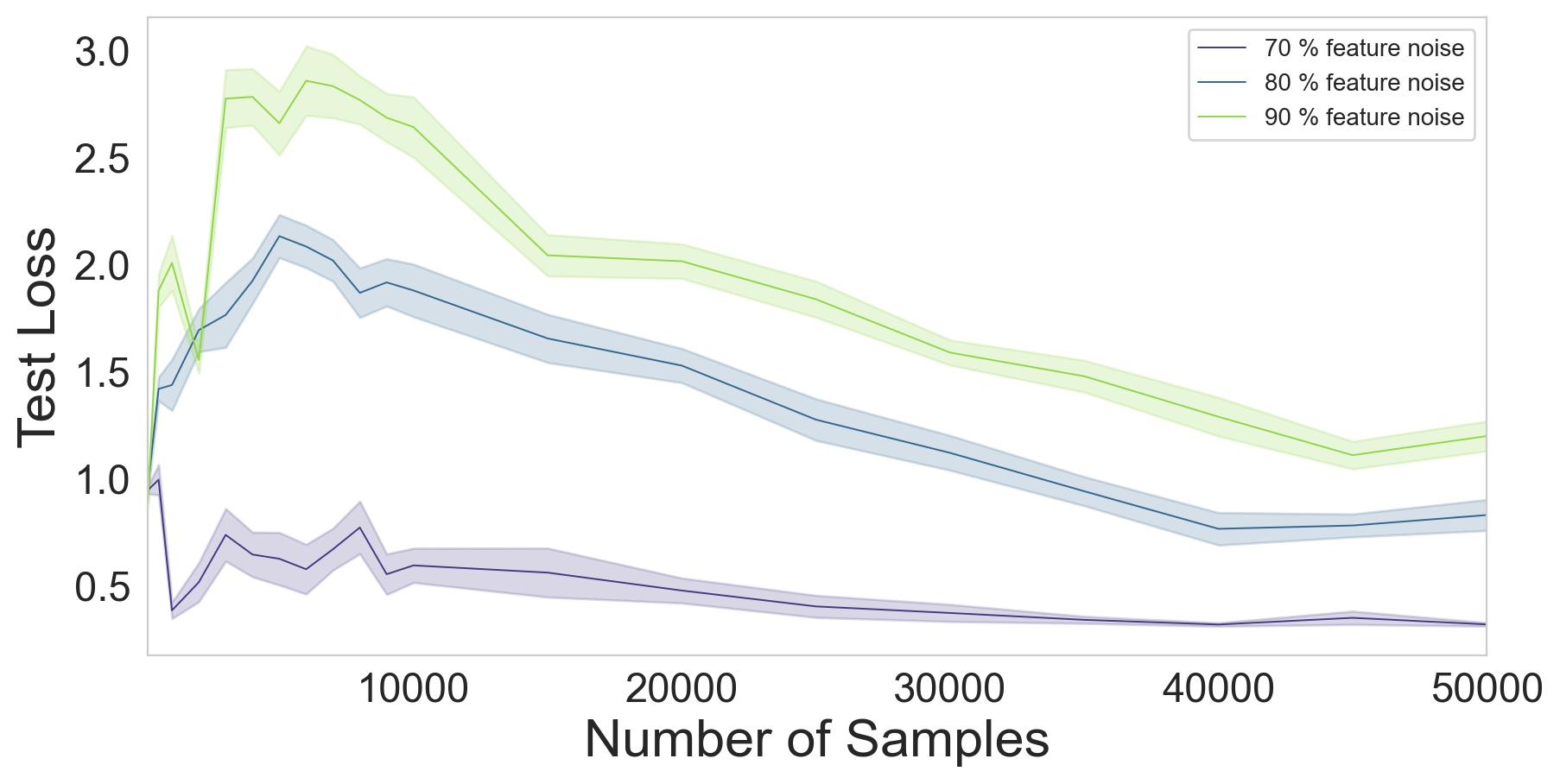
(d) Feature Noise scenario. SNR = -13 [dB].

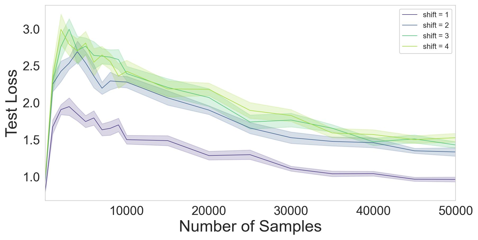
(e) Varying domain shifts.

Figure 15: Sample-wise non-monotonicity and double descent for the linear subspace data. Results for the training losses are in Appendix C, Figure 34.

5 Real World Applications

In this section, we demonstrate how our findings can be applied to important tasks in machine learning, such as domain adaptation and anomaly detection. Our objective is to emphasize the significance of model size selection rather than to compete with state-of-the-art techniques.

5.1 Domain Adaptation

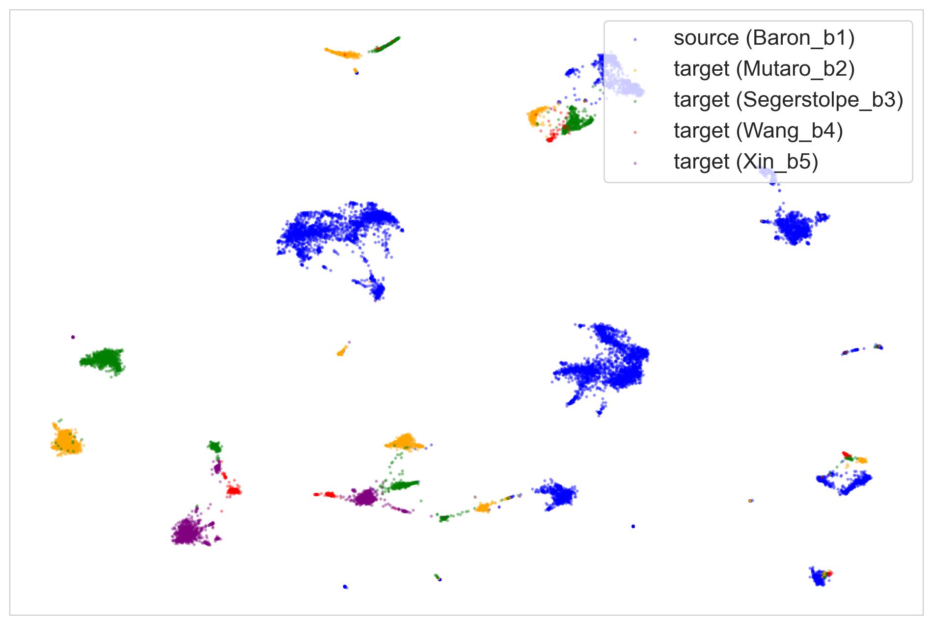
Figure 16: UMAP representations of source and target datasets for the single-cell RNA dataset. Each cluster represents a different cell type. A shift exists between different domains represented by different colors.

Many frameworks in machine learning are exposed to domain shifts as discussed in Section 4.1. The difference in distribution between the training and testing data can lead to inferior results when the model is employed on new, unseen data. Over the years, numerous domain adaptation methods have been proposed for both supervised and unsupervised settings [33, 34, 35, 36, 37] to minimize the shift between the source and target domains. This is an ongoing challenge in biology, where researchers attempt to integrate datasets collected under different environmental conditions that cause distribution shifts. Numerous studies have been conducted to develop strategies to mitigate this shift, known in biology as "batch effect" [32].

In this section, we study the relation between model size and its ability to alleviate distribution shifts in real world single-cell RNA data 3.2. UMAP representations [38] of the source and target datasets are presented Figure 16. The top two sub-figures in Figure 17 present the test and train losses, respectively, for models trained on source and tested on target datasets. We observed that ’Wang’ dataset results in triple descent, while all other targets result in double descent curves.

To evaluate how different models perform in terms of domain adaptation, we measure how much of the domain shift was removed by analyzing the bottleneck representations of the AEs. Precisely, we compute the $k=10$ nearest neighbors of each bottleneck vector and determine the proportion belonging to the same biological batch as mentioned in [39], Section 3. We call this metric “k-nearest neighbors domain adaptation test" (KNN-DAT), indicating the extent of mixing between the source and target data. KNN-DAT close to 1 implies complete separation, while a lower value indicates better mixing of different domains. That is, lower values of KNN-DAT imply that the embedding of samples from the target domain is more similar to the embedding of samples from the source domain.

In the bottom row of Figure 17 we present the UMAP representations extracted based on the embeddings of the learned AEs. For small models, KNN-DAT results are better compared to the interpolating models. However, they achieve lower KNN-DAT at the expense of learning the source data inadequately (high train loss), which is the primary objective of the learning process. The interpolating models fit the source data, preventing them from learning any shared representations of the different batches, resulting in high KNN-DAT. We find that over-parameterized models yield the best KNN-DAT results, achieving a score of 0.75 with a hidden layer size of 2000. Over-parameterized models also lead to reduced train and test losses, resulting in improved reconstruction of both the source and target data. This suggests that over-parameterized models facilitate the transition between source and target datasets, serving as a viable domain adaptation strategy. We also display results for the linear subspace dataset in Appendix D.

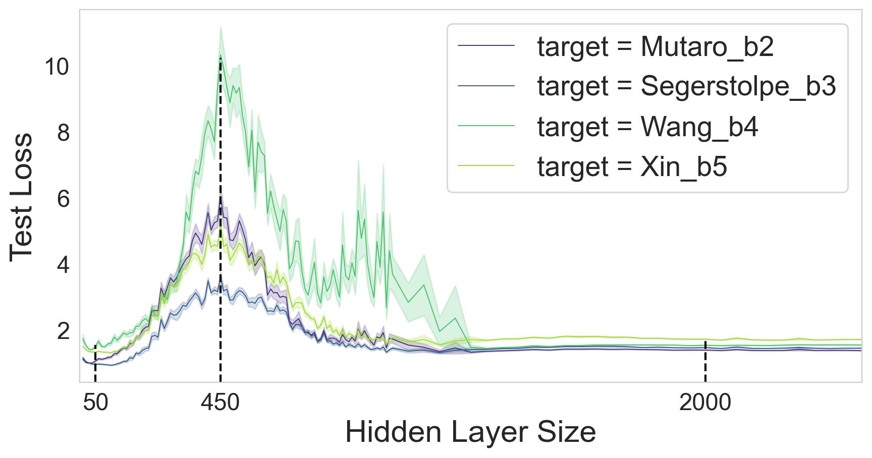
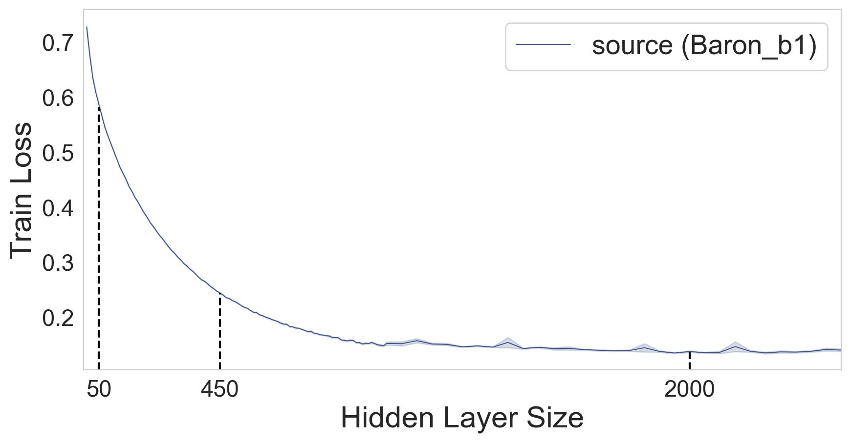
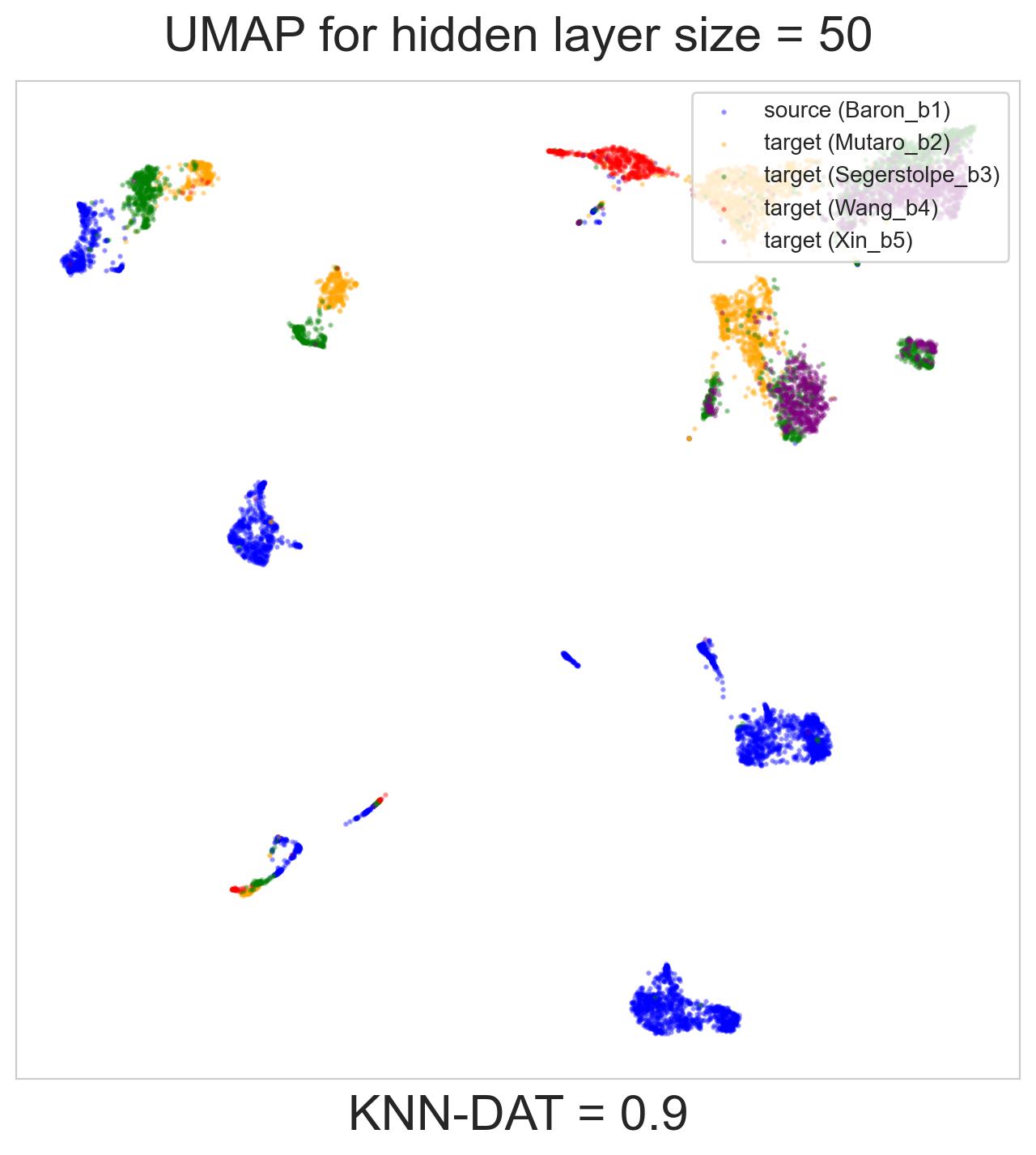
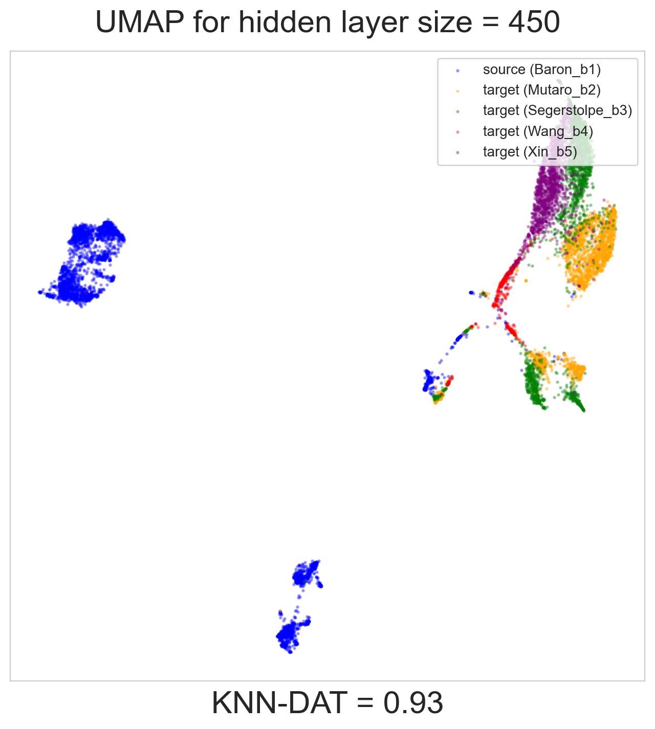
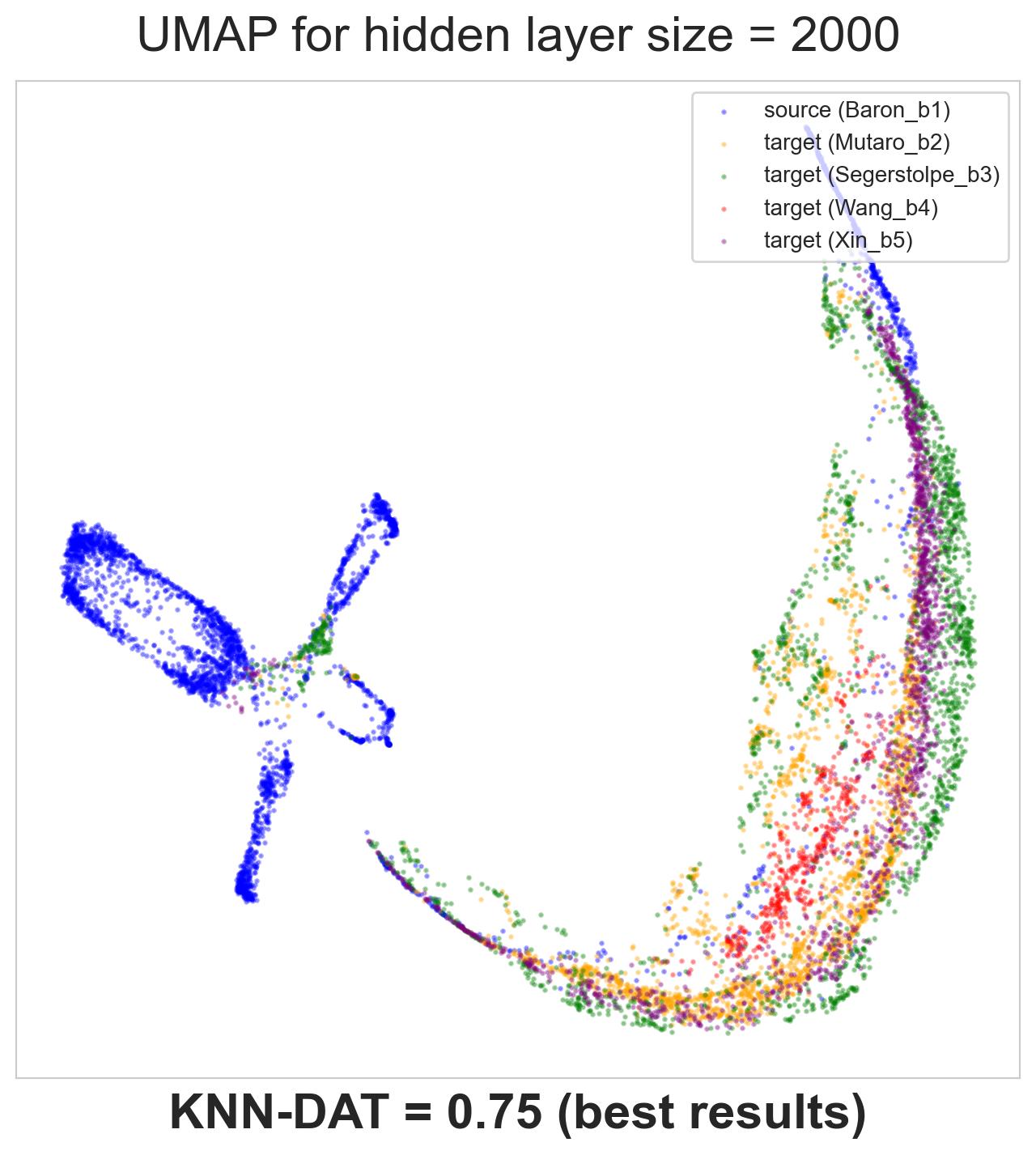
Figure 17: UMAP of latent (bottleneck) vectors of size 300 extracted from the encoder’s output and KNN-DAT results for different model sizes trained on the single-cell RNA dataset.

5.2 Anomaly Detection

Unsupervised anomaly detection is a vital task in machine learning [40, 41, 42, 43], which finds numerous applications across all scientific fields. Several studies have used under or over complete AEs for detecting anomalies. We incorporate real-world data to investigate anomaly detection across various model sizes. Specifically, we leverage the CelebA attributes dataset used in [44], comprising over 200K samples and 4,547 anomalies, each characterized by 39 attributes. We conducted an experiment similar to the one in Section 4.1 to investigate how the size of a model affects its ability to detect anomalies. As expected, in line with findings from [44], small models outperform larger models in anomaly detection (see the decrease in ROC-AUC in Figure 18). In contrast to the experiment in Section 4.1, we do not control the SAR value in this data. Since the SAR is positive, we do not observe a double descent in the test loss curves. Nonetheless, we identify a non-monotonic behavior of the ROC-AUC curve. Initially, it decreases for intermediate models, followed by an increase for over-parameterized models. In conclusion, when employing a model for unsupervised anomaly detection, it is recommended to avoid selecting intermediate models, as their anomaly detection performance is inferior to under and over-parameterized models.

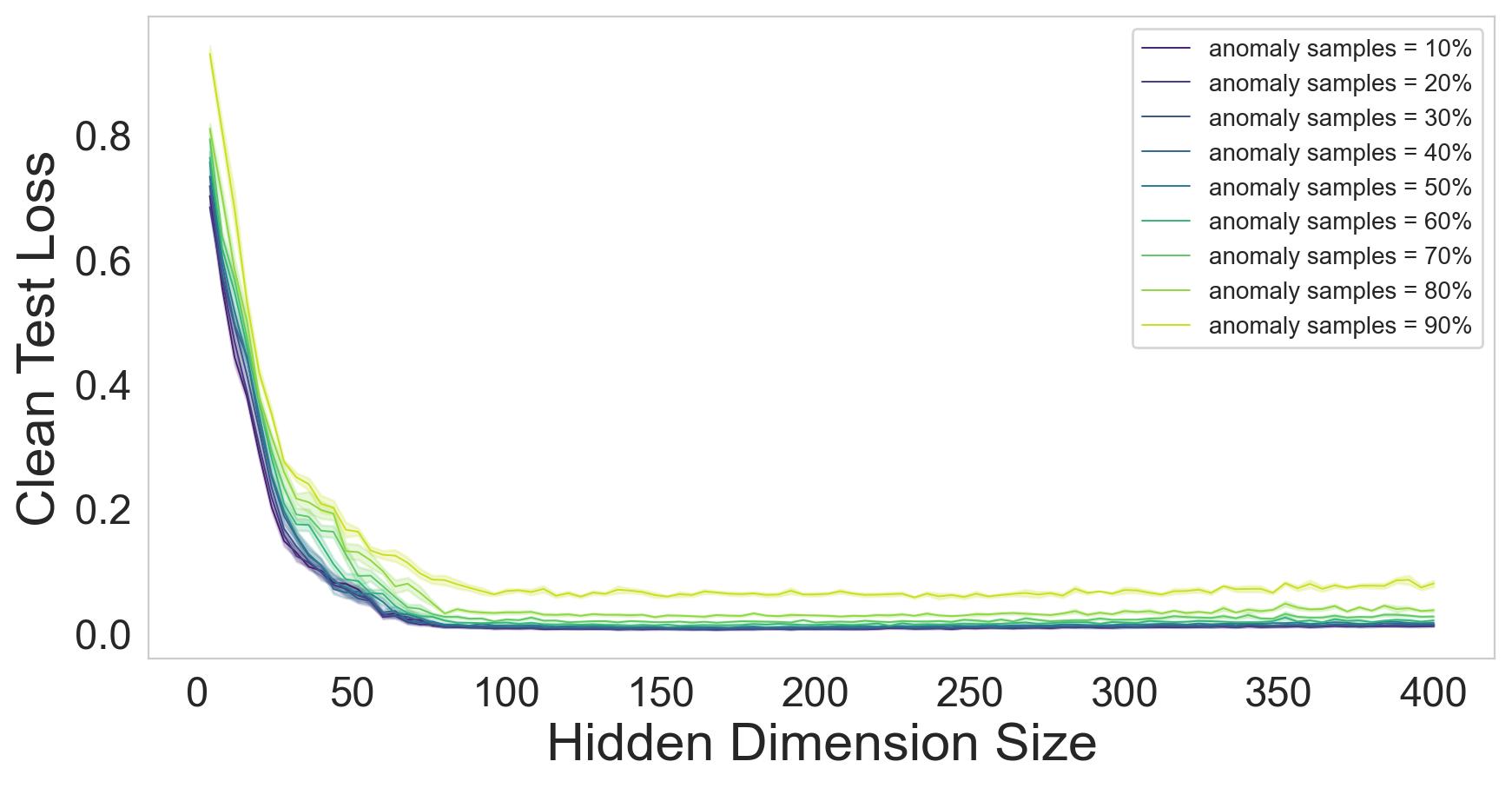
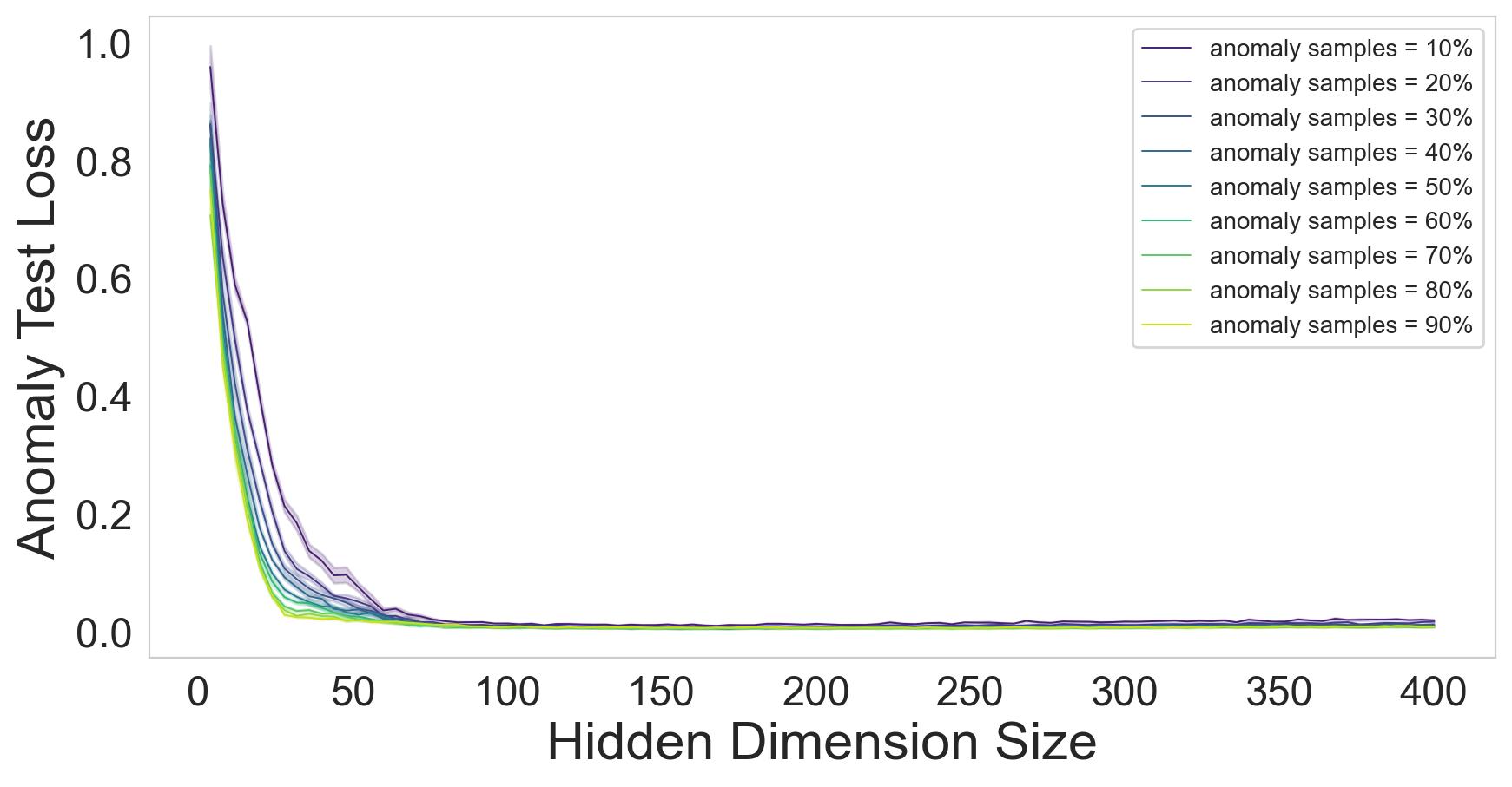
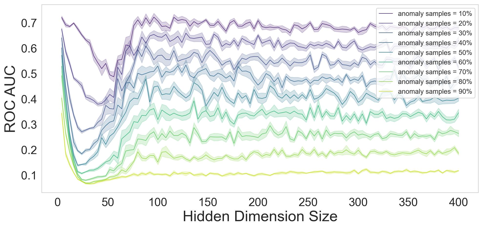
Figure 18: Left, middle: test loss of clean and anomaly data respectively. Right: non-monotonic behavior of the ROC-AUC for the celebA dataset.

6 Conclusions

In our study, we identified various instances of multiple descents and non-monotonic behaviors in unsupervised learning. These phenomena occur at the model-wise, epoch-wise, and sample-wise levels. We used under-complete autoencoders (AE) to investigate these phenomena and found compelling evidence for their robustness across diverse datasets, training methodologies, and experimental scenarios. We examined four distinct use cases: sample noise, feature noise, domain shift, and anomalies. Our experiments revealed multiple instances of consecutive descents, with some resulting in improved (lower) test loss. Additionally, we found a connection between the size of the model and its real-world performance. Specifically, over-parameterized models can serve as effective domain adaptation strategies when there is a distribution shift between the source and target data. In the realm of anomaly detection, we find that it is important to avoid selecting intermediate models that yield lower ROC-AUC outcomes. The limitations of our work lie in the utilization of a certain (yet, prototypical) type of fully connected AE model. Future work could focus on formulating theories to interpret the phenomena outlined in our findings.

Appendix A Implementation Details

In this section, we provide complete implementation details for all experiments conducted in the paper. Illustrations of the synthetic data generation introduced in Section 3.1 for the scenarios of sample noise, feature noise, domain shift, and anomalies are displayed in Figures 19, 20, 21 respectively.

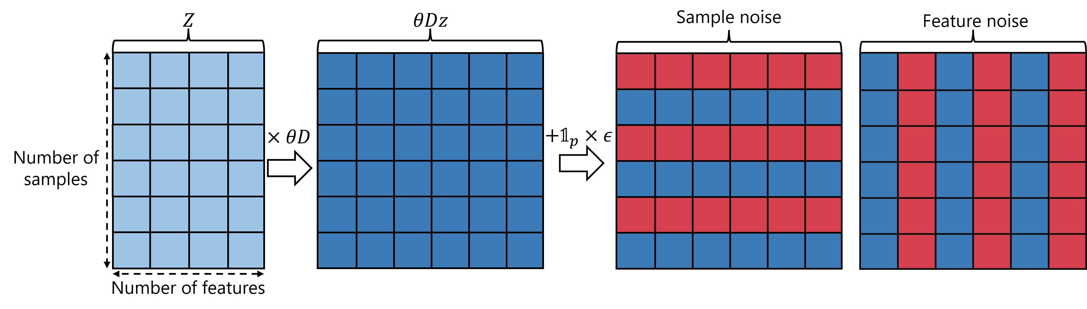
Figure 19: Data generation for the scenarios of sample and feature noise with $p=0.5$. The first (leftmost) matrix depicts the latent vectors $Z$. The second matrix illustrates the latent vectors being projected into a higher dimensional space, and the rightmost matrices contain clean (blue) and noisy (red) samples / features respectively.

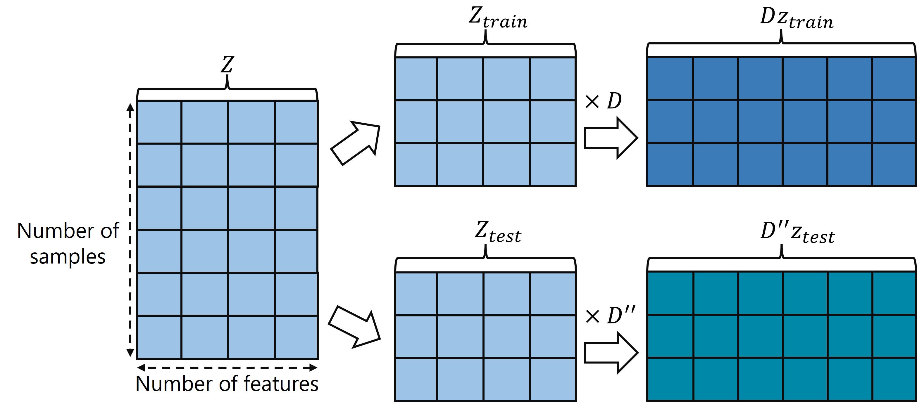
Figure 20: Data generation for the scenario of domain shift. The matrix on the left depicts the latent vectors $Z$ and the two middle matrices represent the separation to source ($Z_{train}$) and target ($Z_{test}$). The two rightmost matrices illustrate the latent vectors of the train and test data being projected into a higher dimensional space with different matrices ($D,D^{{}^{\prime\prime}}$), resulting in a domain shift.

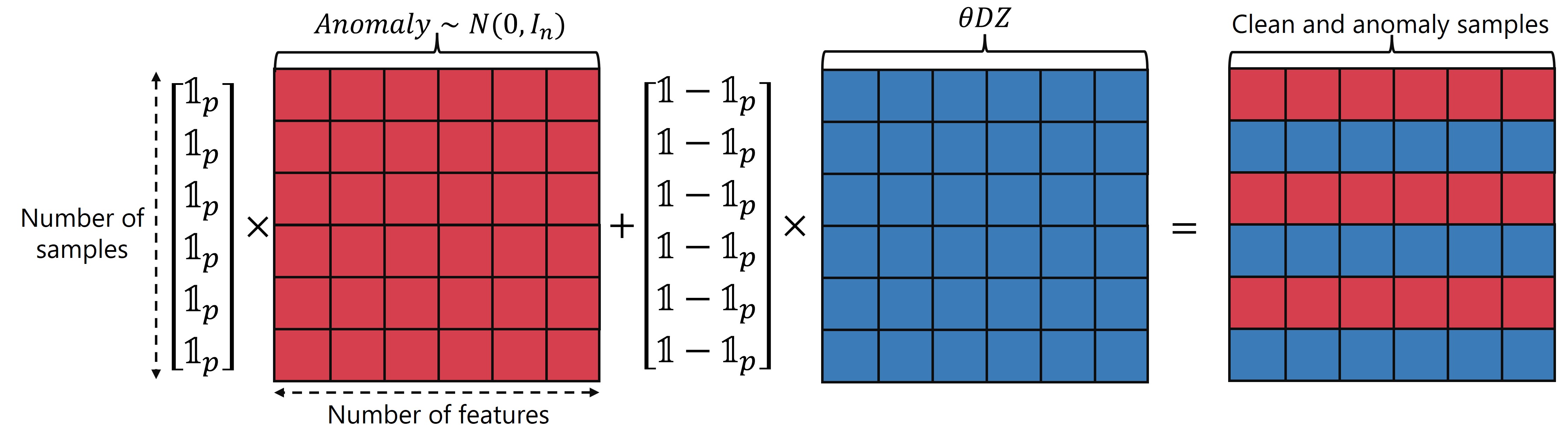
Figure 21: Data generation for the case of anomalies and $p=0.5$. The matrix on the left depicts the anomalous data, the middle matrix represents the clean data, and the rightmost matrix contains both clean (blue) and outlier (red) samples.

Parameters.

Table 1 details the hyper-parameters for the training process and other parameters employed for the linear subspace and single-cell RNA datasets. The training optimizer utilized was Adam [45], and the loss function for reconstruction is the mean squared error, which is mentioned in this Section.

Table 1: Parameters and hyper-parameters.

Parameters	Linear Subspace Dataset Values	Single-Cell RNA Dataset Values
Learning rate	0.001	0.001
Optimizer	Adam	Adam
Epochs	200	1000
Batch size	10	128
Data’s latent size ($d$)	20	-
Number of features ($n$)	50	1000
Train dataset size	5000	5000
SNR [dB]	-20, -15, -10, -7, -5, -2, 0, 2	-20, -15, -10, -7, -5, -2, 0, 2
Sample/ feature noise ($p$)	0, 0.1, 0.2,…,1	0, 0.1, 0.2,…,1
Domain shift scale ($s$)	1, 2, 3, 4	-
Bottleneck layer size	25, 30, 45	20, 100, 300
Hidden layer size	4 - 500	10 - 3000

Model.

All experiments are conducted with the same multi-layer perceptron under-complete AE. The objective is to prevent the model from learning the identity function and instead encourage the acquisition of a meaningful embedding in the latent space. To facilitate the exploration of double descent in both bottleneck layer size and hidden layer size, we employ a simplified model consisting of a single hidden layer for both the encoder and decoder, as depicted in Figure 22. The size of the model is determined by the sizes of the hidden layers and the bottleneck layer, while the width of the model remains constant.

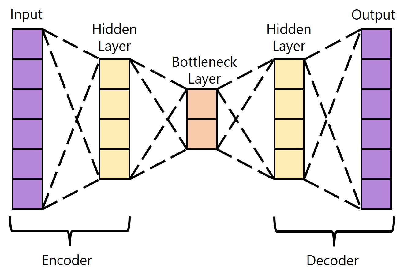
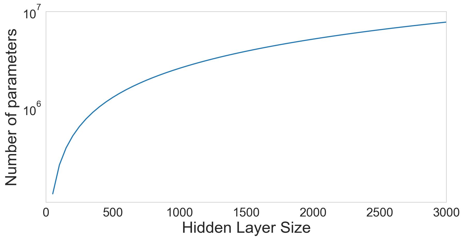
Figure 22: Left: Demonstration of the model structure. Right: model’s number of parameters for single-cell RNA settings (bottleneck layer size = 300 and input size = 1000 features).

Loss function.

All AEs are trained with the mean squared error (MSE) loss function:

$$\text{MSE}=\frac{1}{n}\sum_{i=1}^{n}(y_{i}-\hat{y}_{i})^{2}.$$

Where $n$ is the number of data samples, $y_{i}$ is the true value, and $\hat{y}_{i}$ is the predicted value. Due to contamination in the training dataset, the norm of train samples tends to be higher than that of the clean test samples. As the MSE loss is not scale-invariant, we opt to normalize both train and test losses only after the training process is complete, using $\frac{1}{n}\sum_{i=1}^{n}(y_{i}-\bar{y})^{2}$, Where $\bar{y}$ is the mean of $\{y_{i}\}_{i=1}^{n}$. This strategy enables us to continue utilizing the MSE loss function while facilitating a fair and meaningful comparison between train and test losses.

Results.

Ensuring the robustness of the findings across various model initializations and enhancing their reliability, all figures combine several results of different random seeds. The bolded curves in each figure represent the average across the results of different seeds, and the transparent curve around the bolded curve represents the $\pm 1$ standard error from the mean.

Environments and Computational Time.

All experiments were conducted on NVIDIA RTX 6000 Ada Generation with 47988 MiB, NVIDIA GeForce RTX 3080 with 10000 MiB, Tesla V100-SXM2-32GB with 34400 MiB, and NVIDIA GeForce GTX 1080 Ti with 11000 MiB.
Each result in Figure 3 represents an average over 10 seed runs. The hidden layer sizes for the linear subspace data range from 4 to 500 with a step size of 4, and for the single-cell RNA data, they range from 10 to 500 with a step size of 10, and from 500 to 3000 with a step size of 50. This results in 125 and 110 models trained for each dataset, respectively. Figure 3(a) presents 9 different sample noise levels, entailing the training of $125\cdot 10\cdot 9=11250$ models. Each evaluation of a specific sample or feature noise curve involves 1250 trained models, which can take from one day if trained on an NVIDIA RTX 6000 Ada Generation GPU to several days if trained on the other mentioned GPUs to obtain the results.

Appendix B SNR Calculations

In this section, we will outline our approach for calculating the signal-to-noise ratio (SNR) for all experiments involving the addition of noise. Initially, we convert the SNR from decibels to linear SNR using the formula:

$$\text{SNR}=10^{\left(\frac{\text{SNR[dB]}}{20}\right)}.$$ (1)

We have a closed-form equation for the linear subspace dataset to determine the scalar $\theta$ required to multiply the train samples and achieve the desired linear SNR value. We use the fact that both train and noise are sampled from an i.i.d. normal distribution and calculate $\theta$ for the sample noise, feature noise, domain shift, and anomalies.

Notations:
$z-d\times 1$ vector. Represents a vector in a latent space of size $d$.
$D-n\times d$ matrix. Represents a random matrix to project $z$ from a $d$ dimensional space into a higher-dimensional space ($n>d$).
$\epsilon-n\times 1$ vector. Represents the noise added to a vector with $n$ dimensions.

For the scenario of sample noise, where a particular sample is affected by noise across all its features:

$$\text{SNR}^{2}=\frac{E[\|\theta Dz\|_{2}^{2}]}{E[\|\epsilon\|_{2}^{2}]}=\frac{E[\theta^{2}z^{T}D^{T}Dz]}{E[\epsilon^{T}\epsilon]}=\frac{\theta^{2}E_{z}[E_{D|z}[z^{T}D^{T}Dz|z]]}{E\left[\sum_{i=1}^{n}\epsilon_{i}^{2}\right]}\underbrace{=}_{\text{(a)}}$$ (2)

$$\frac{\theta^{2}E_{z}[z^{T}E_{D|z}[D^{T}D]z]}{n}\underbrace{=}_{\text{(b)}}\frac{\theta^{2}E_{z}[z^{T}n\cdot I_{d\times d}z]}{n}=\frac{\theta^{2}\cdot n\cdot E_{z}[z^{T}z]}{n}=\theta^{2}E\left[\sum_{i=1}^{d}z_{i}^{2}\right]\underbrace{=}_{\text{(a)}}\theta^{2}\cdot d.$$

Isolating $\theta$, we get that $\theta=\frac{\text{SNR}}{\sqrt{d}}$.

(a) Given a vector $a\sim\mathcal{N}(0,I_{n})$ of $n$ i.i.d. samples, $E\left[\sum_{i=1}^{n}a_{i}^{2}\right]=\sum_{i=1}^{n}E[a_{i}^{2}]=\sum_{i=1}^{n}1=n$.

(b) Given a matrix $M\sim\mathcal{N}(0,I_{n})$ of size $n\times n$ where all entries are i.i.d., then
$E[M^{T}M]=E\begin{bmatrix}M_{1,1}^{2}+\dots+M_{n,1}^{2}&\dots&M_{1,1}M_{1,n}+\dots+M_{n,1}M_{n,n}\\ \vdots&\ddots&\vdots\\ M_{1,1}M_{1,n}+\dots+M_{n,1}M_{n,n}&\dots&M_{1,n}^{2}+\dots+M_{n,n}^{2}\end{bmatrix}=\begin{bmatrix}n&\dots&0\\ \vdots&\ddots&\vdots\\ 0&\dots&n\end{bmatrix}=n\cdot I_{n\times n}$.

For the scenario of feature noise, each train sample has only $n\cdot p$ noisy features, meaning the noise vector contains values for only $n\cdot p$ entries. Consequently, $\theta$ is determined by $\sqrt{\frac{p}{d}}\cdot\text{SNR}$. For practitioners who want to explore the scenario involving domain shift, where the source and target are noisy, note that the matrix responsible for projecting $z_{test}$ into a higher-dimensional space is denoted as $D^{{}^{\prime\prime}}=D+s\cdot D^{{}^{\prime}}$ where $D^{{}^{\prime}}$ is sampled from a standard normal distribution $\mathcal{N}(0,I)$ and both $D$ and $D^{{}^{\prime}}$ are i.i.d. Consequently, $D_{ij}^{{}^{\prime\prime}}\sim\mathcal{N}(0,1+s^{2})$. Substituting $D$ with $D^{{}^{\prime\prime}}$ in equation (2), we find that $E_{D^{{}^{\prime\prime}}|z}[D^{{}^{\prime\prime}T}D^{{}^{\prime\prime}}]=n\cdot(1+s^{2})\cdot I_{d}$, leading to $\text{SNR}^{2}=(1+s^{2})\cdot\theta^{2}\cdot d$, therefore $\theta=\frac{\text{SNR}}{\sqrt{(s^{2}+1)d}}$. In other words, since the covariance matrix of $D^{{}^{\prime\prime}}$ is $(1+s^{2})I$, we need to make sure we first normalize the matrix by $\sqrt{1+s^{2}}$ to maintain the identity covariance matrix.

For other datasets, such as the single-cell RNA dataset, we normalize each sample $x$ by its norm $\|x\|$, and similarly normalize each noise vector $n$, yielding: $\hat{x}=\dfrac{x}{\|x\|}$ and $\hat{n}=\dfrac{n}{\|n\|}$. This ensures that the ratio $\dfrac{\hat{x}}{\hat{n}}$ equals 1. By employing equation (1), we attain the intended linear SNR factor $\theta$, and then scale down $\hat{n}$ by $\theta$, yielding $\hat{n}_{scaled}=\dfrac{\hat{n}}{\theta}$. This guarantees that the linear SNR is $\dfrac{\hat{x}}{\hat{n_{scaled}}}=\theta$.

Appendix C Train Loss Results

In this section, we provide the train loss figures corresponding to each of the test losses mentioned in the main paper.

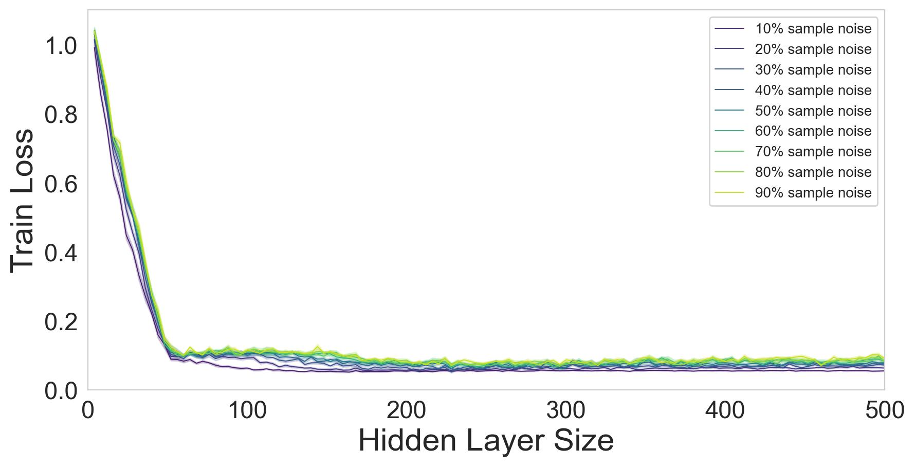
(a) Linear subspace data with SNR = -15 [dB].

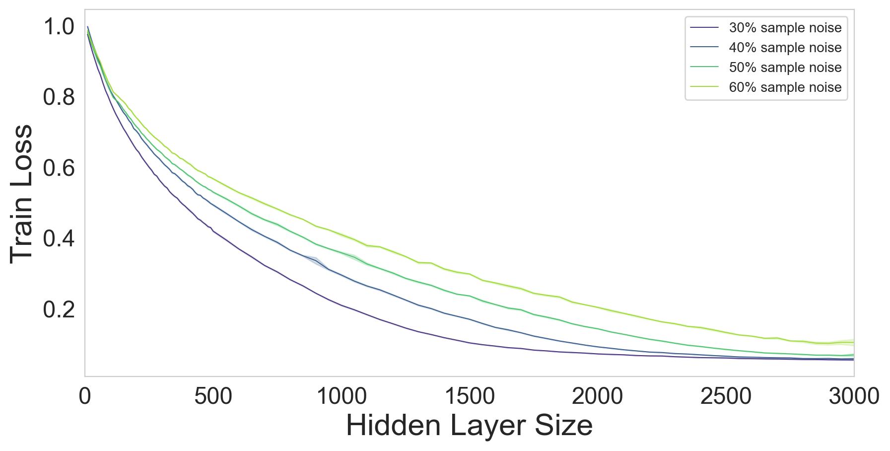
(b) Single-cell RNA data with SNR = -17 [dB].

Figure 23: Model-wise train losses for the case of varying sample noise.

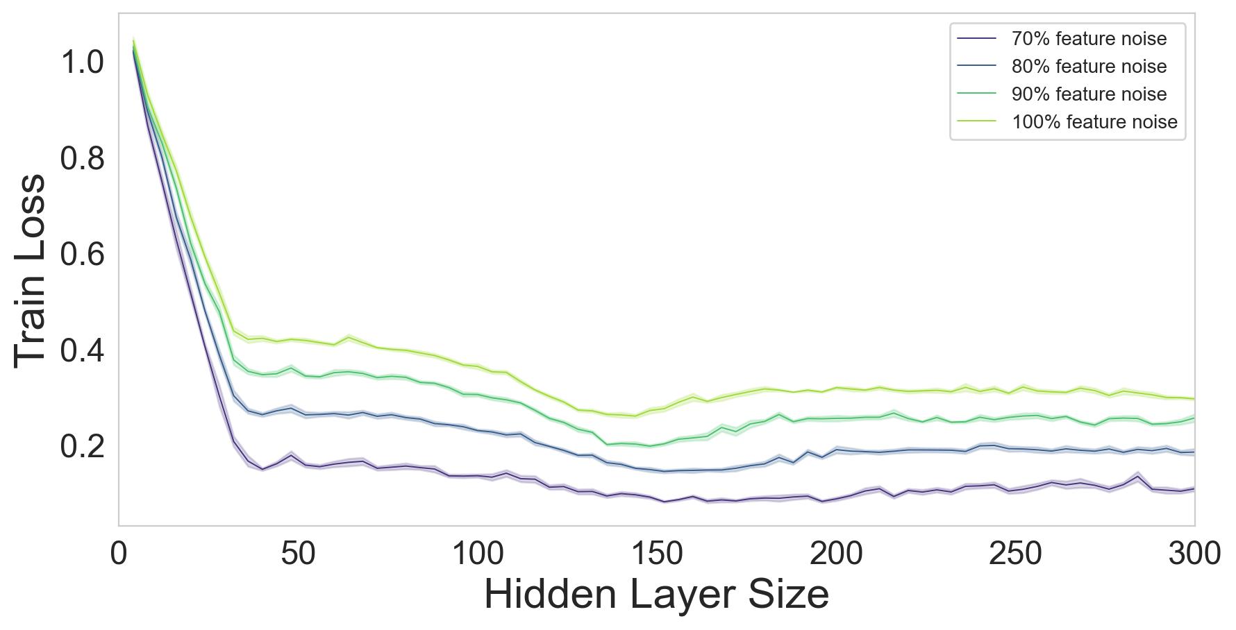
(a) Linear subspace data with SNR = -13 [dB].

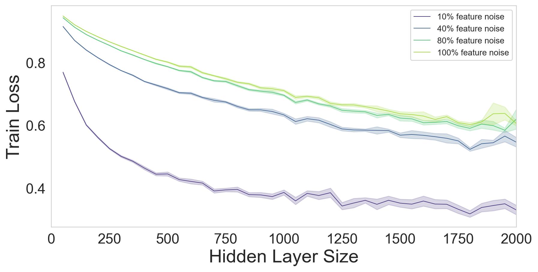
(b) Single-cell RNA data with SNR = -12 [dB]. Train loss increases beyond a hidden layer of 2000.

Figure 24: Model-wise train losses for the case of varying feature noise.

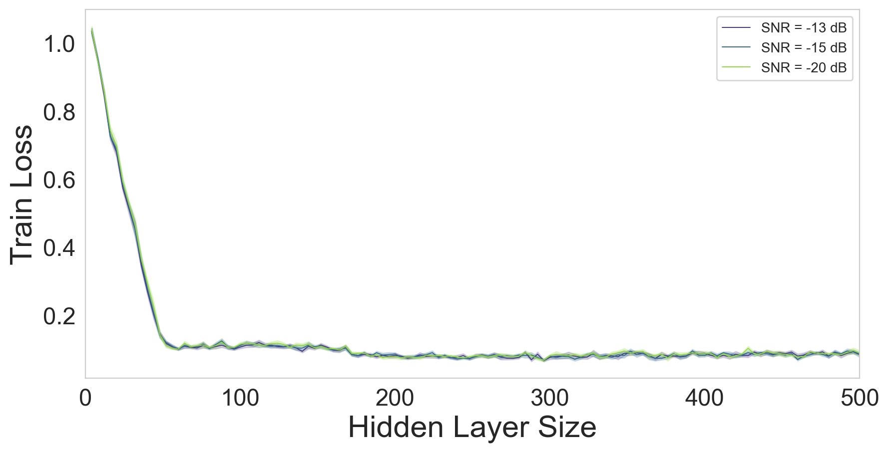
(a) Linear subspace data. Sample noise = 80%.

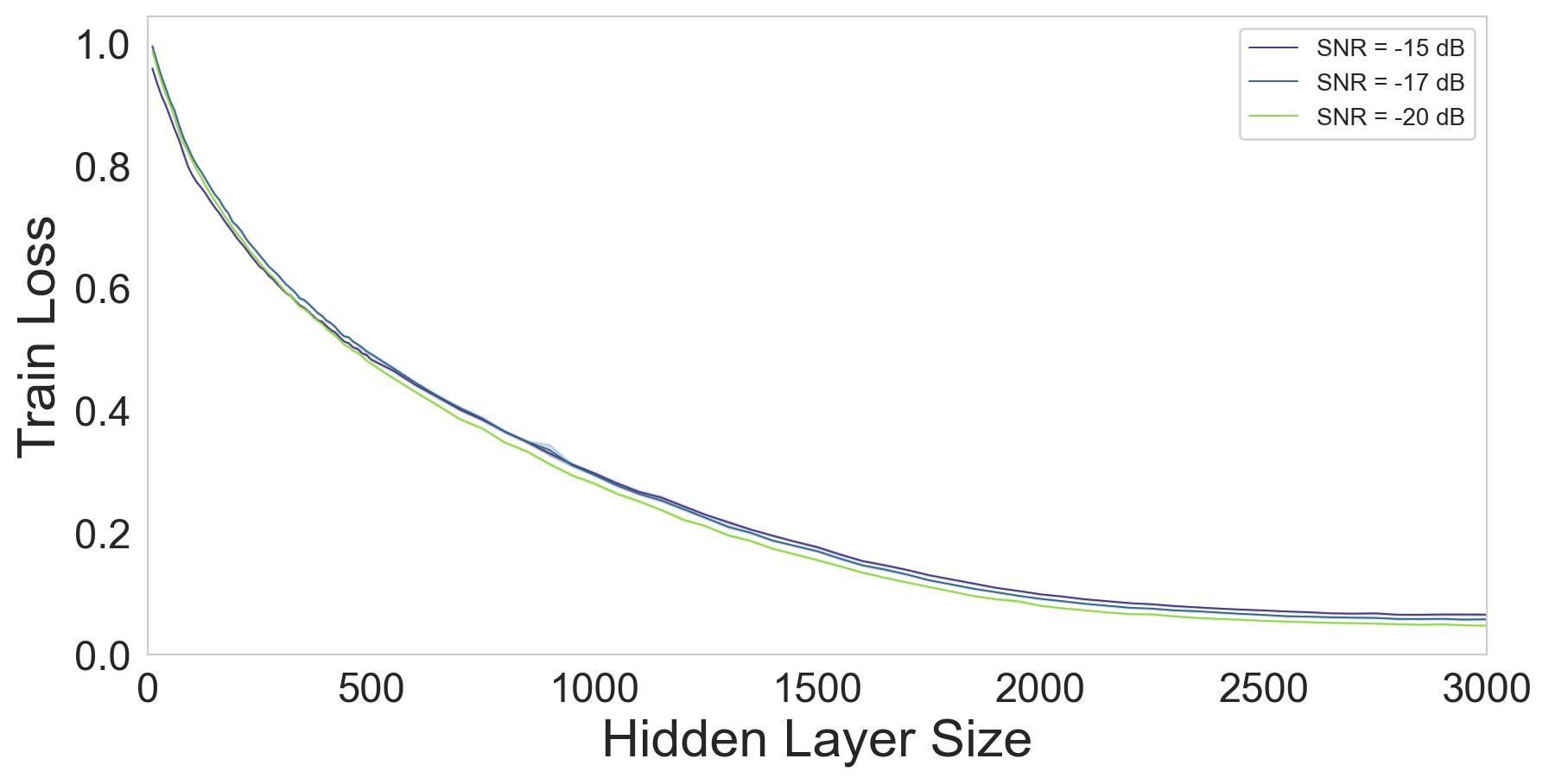
(b) Single-cell RNA data. Sample noise = 40%.

Figure 25: Model-wise train losses for the case of noisy samples and varying SNR.

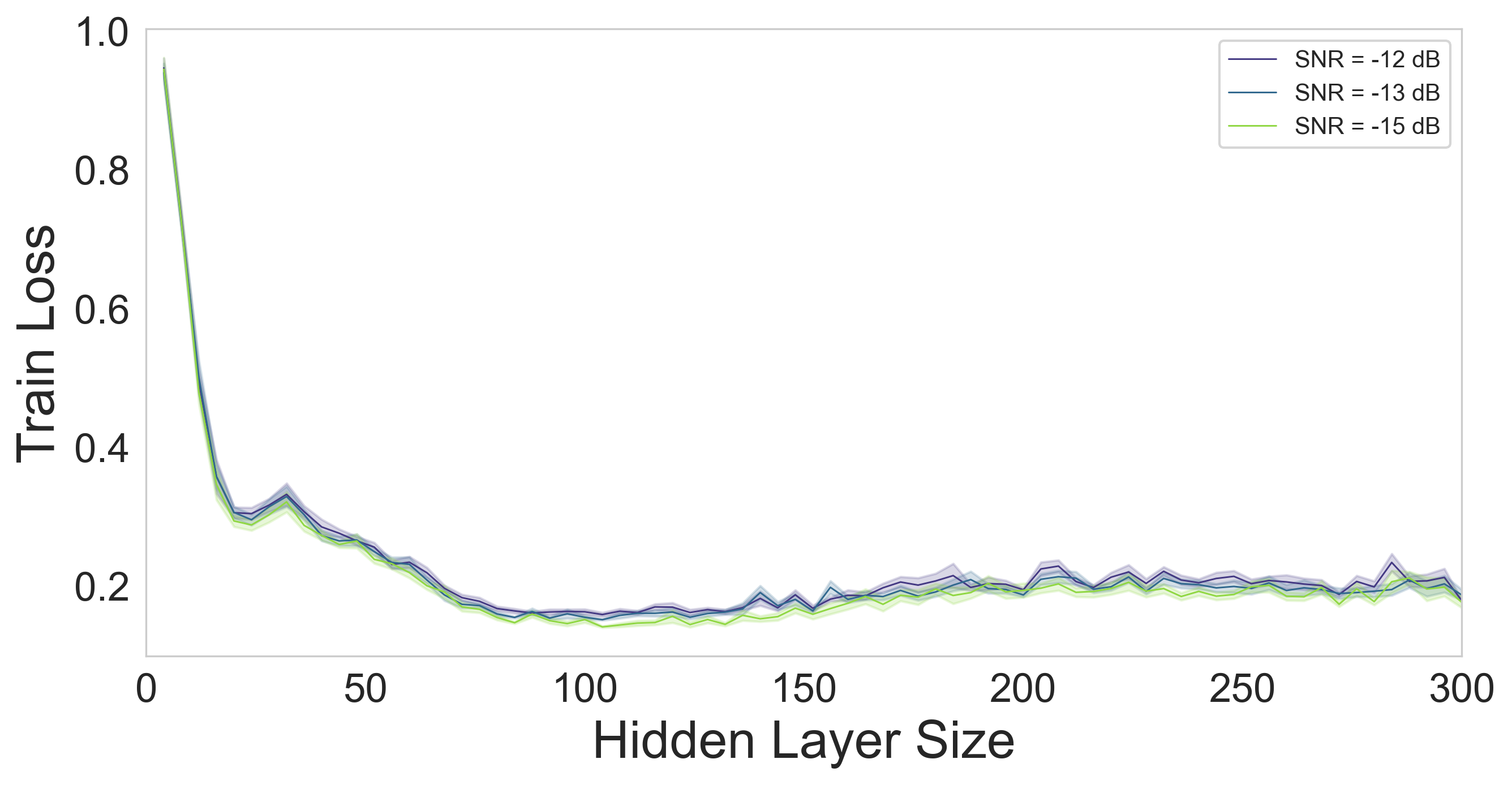
(a) Linear subspace data. 40% noisy features.

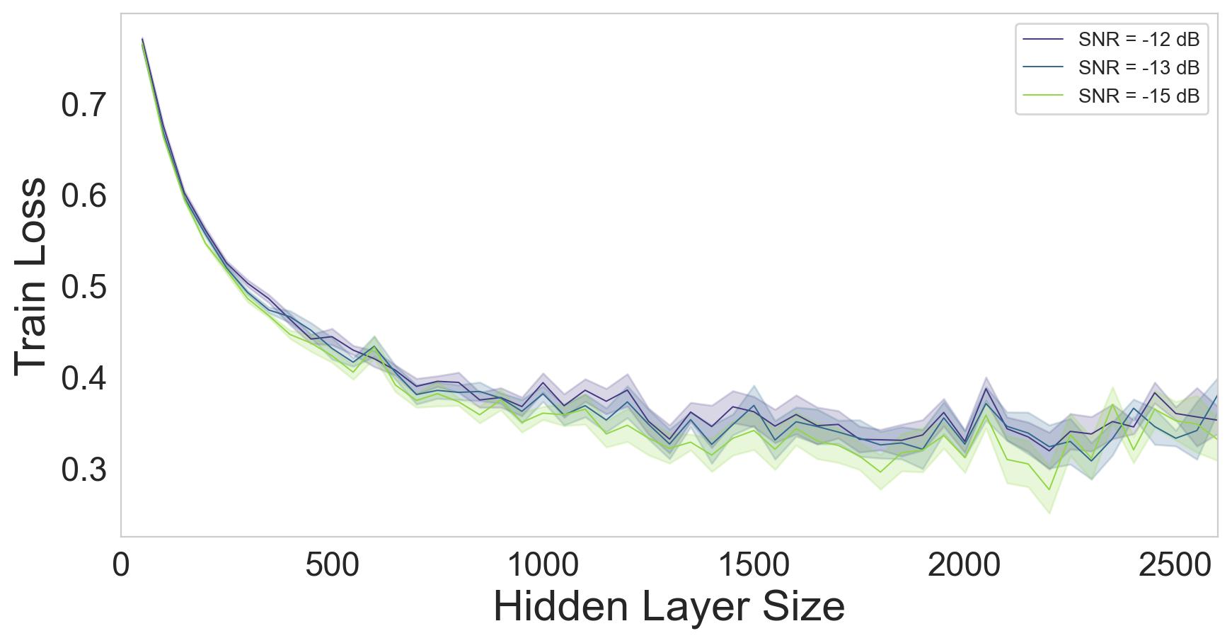
(b) Single-cell RNA data. 10% noisy features. Train loss increases beyond a hidden layer of 2600.

Figure 26: Model-wise train losses for the case of noisy features and varying SNR.

figurec

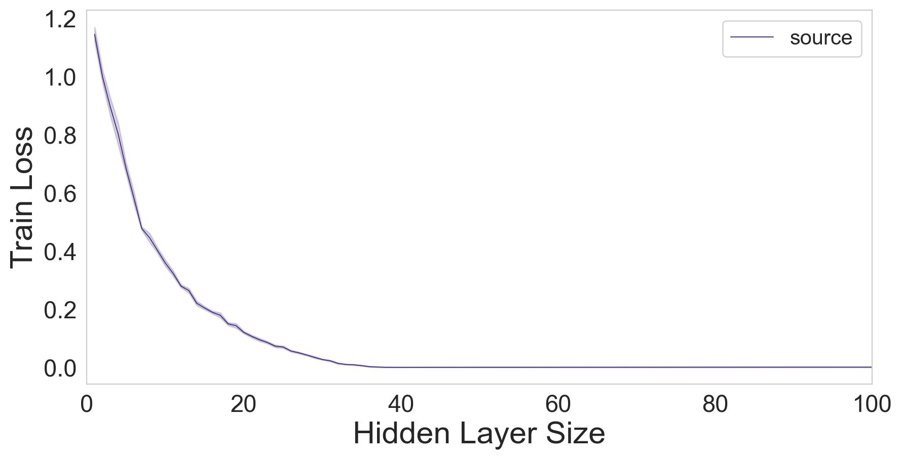
Figure 27: Train loss of source data for the linear subspace data.

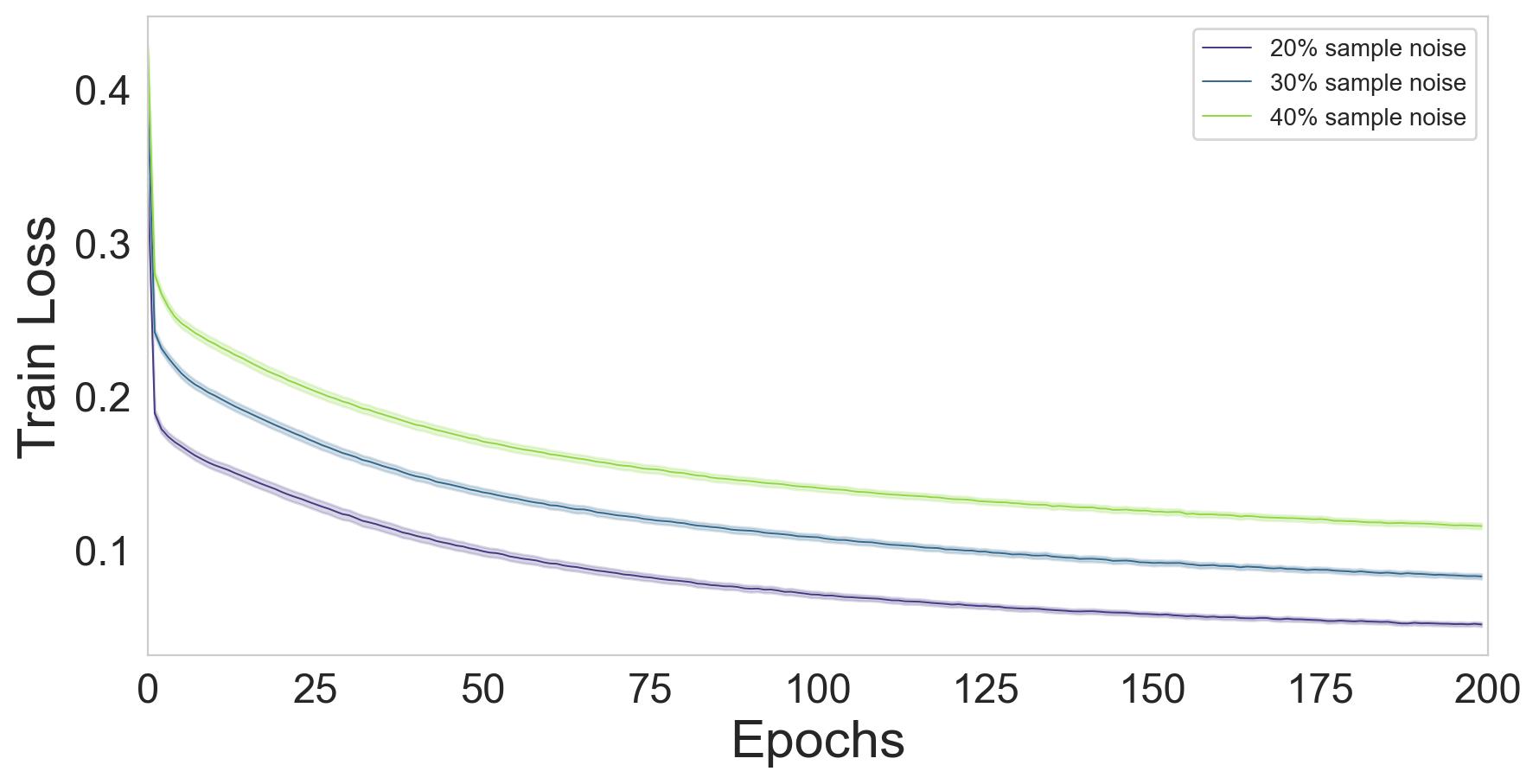
(a) Linear subspace data with SNR = -2 [dB].

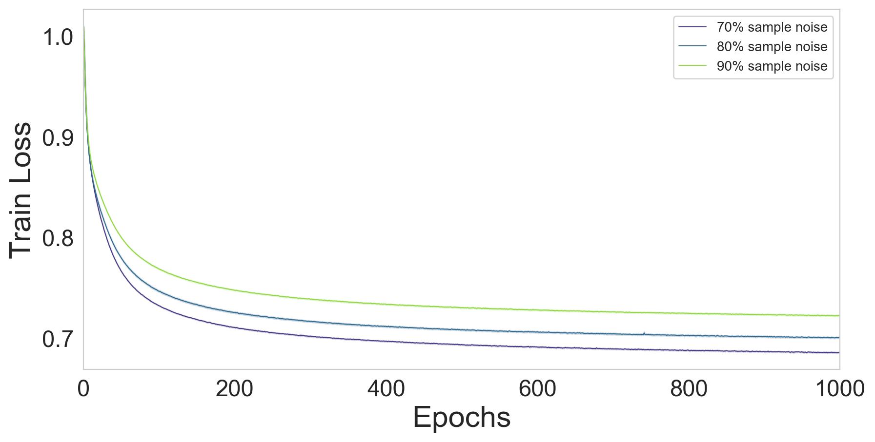
(b) Single-cell RNA data with SNR = -17 [dB].

Figure 28: Epoch-wise train losses for varying number of noisy samples.

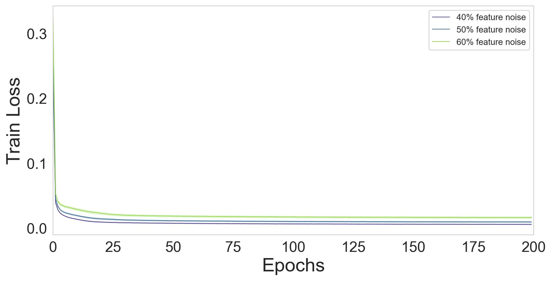
(a) Linear subspace data with SNR = -12 [dB].

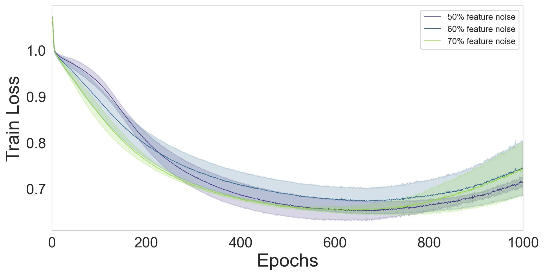
(b) Single-cell RNA data with SNR = -12 [dB].

Figure 29: Epoch-wise train losses for varying number of noisy features.

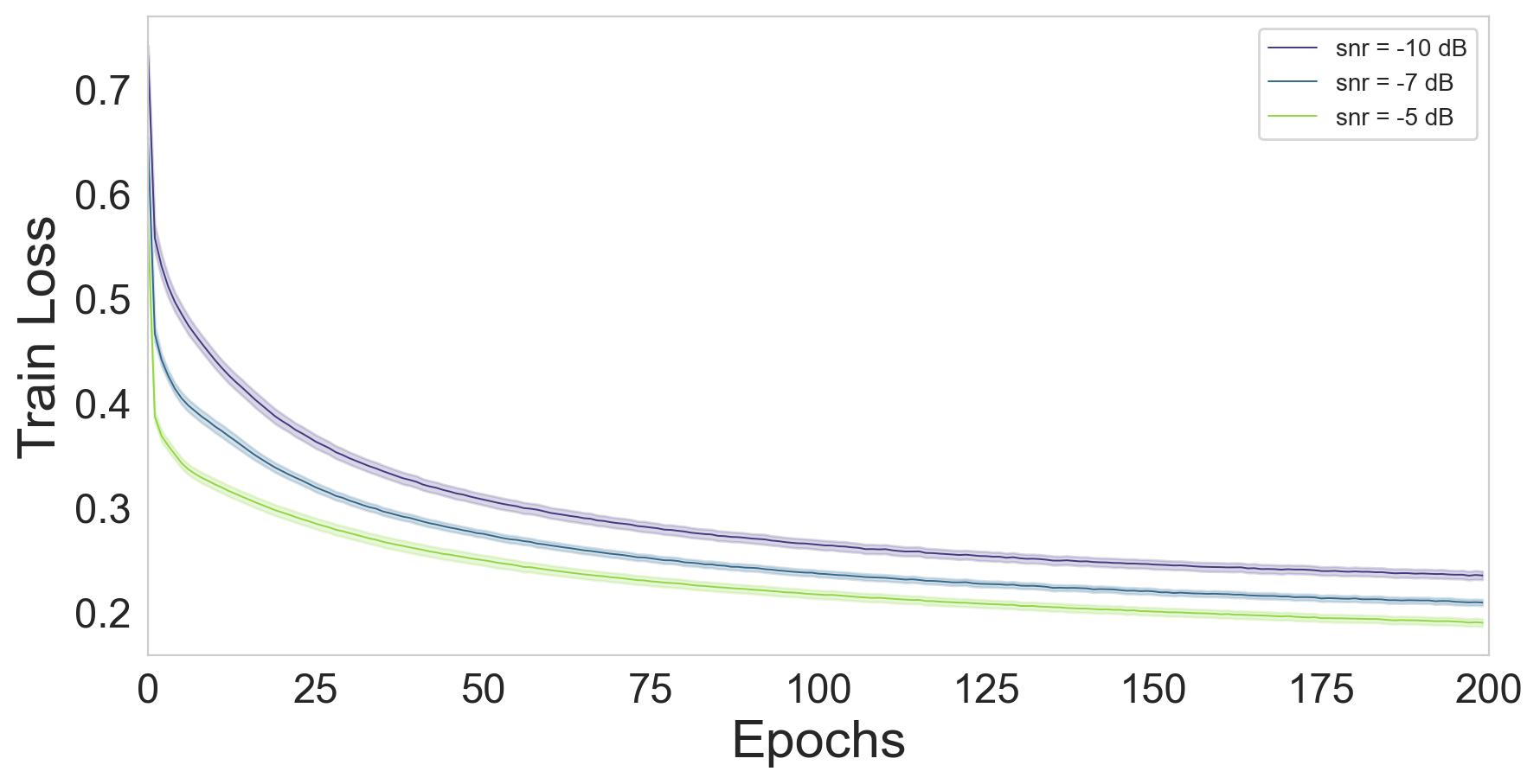
(a) Linear subspace data. Sample noise = 40%.

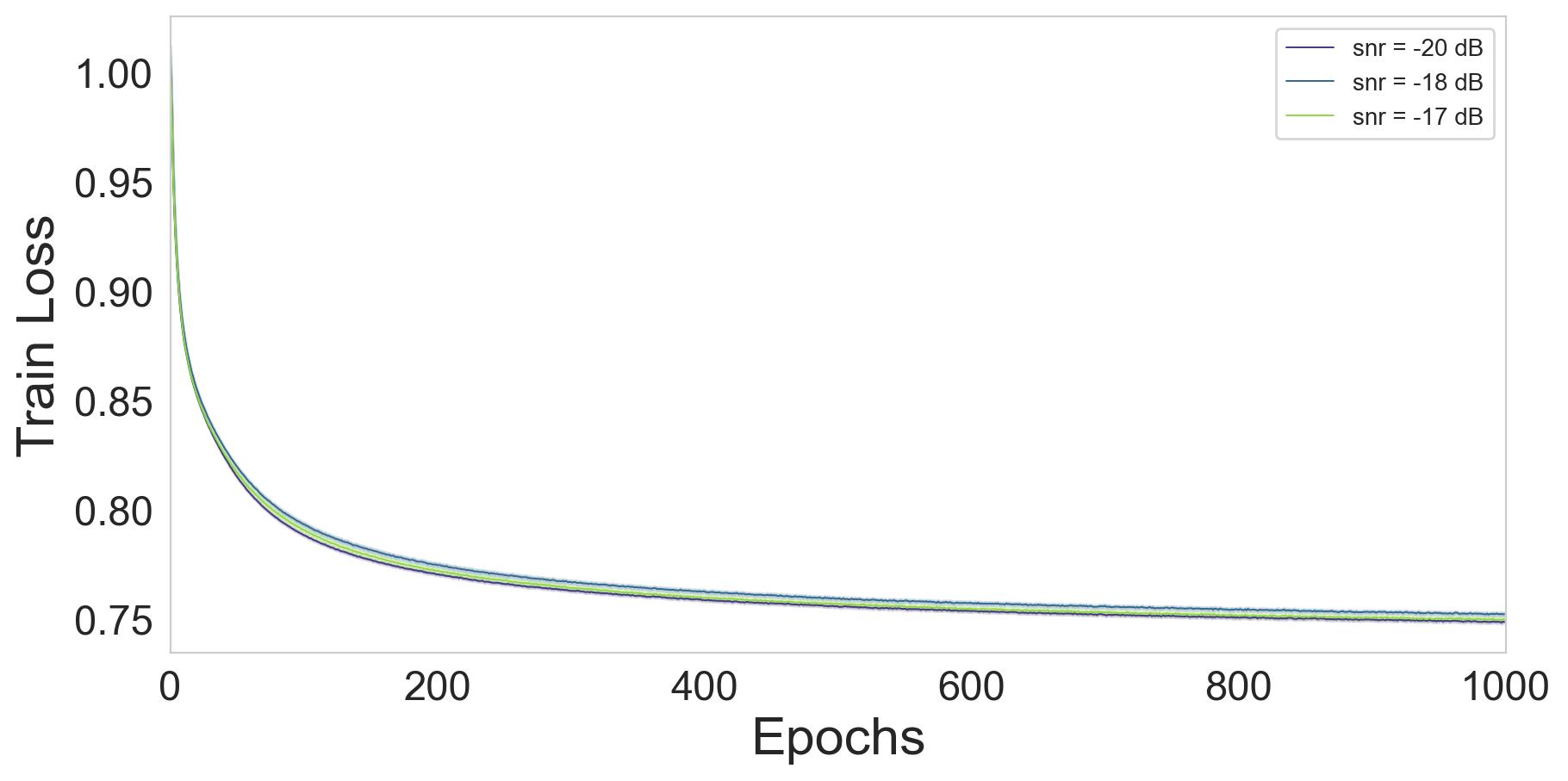
(b) Single-cell RNA data. Sample noise = 90%.

Figure 30: Epoch-wise train losses for the case of sample noise influenced by the SNR.

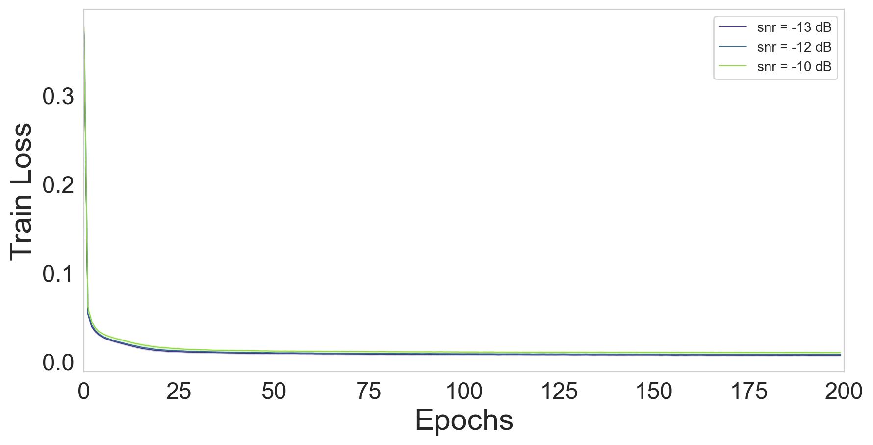
(a) Linear subspace data. Feature noise = 80%.

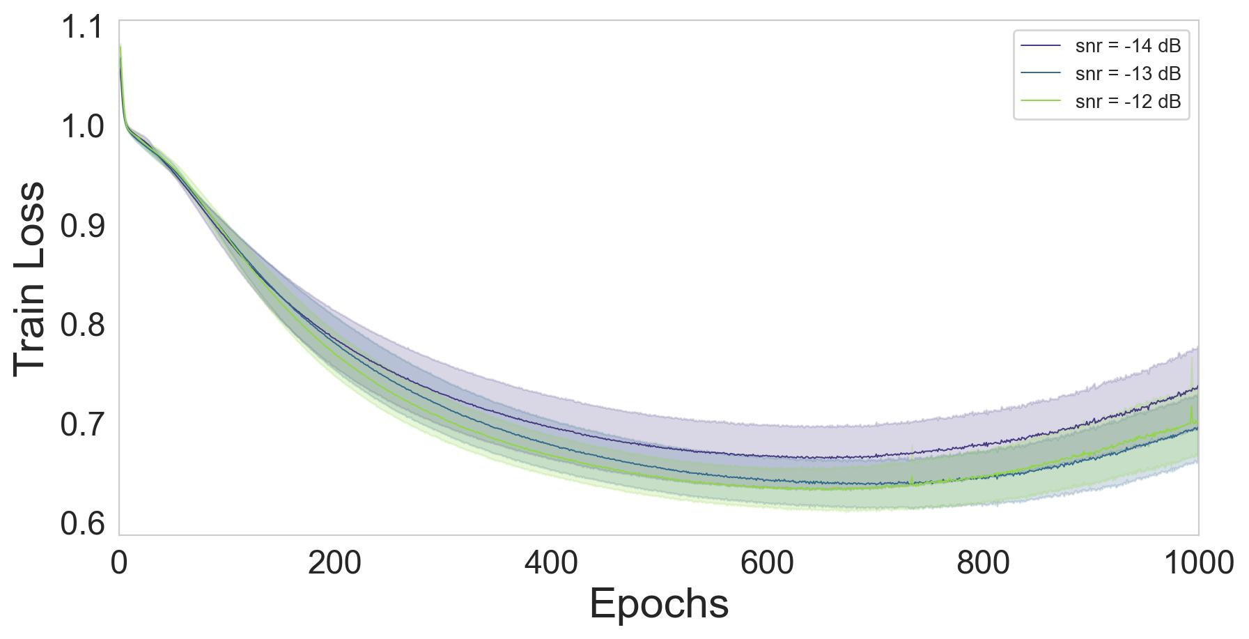
(b) Single-cell RNA data. Feature noise = 50%.

Figure 31: Epoch-wise train losses for the case of feature noise influenced by the SNR.

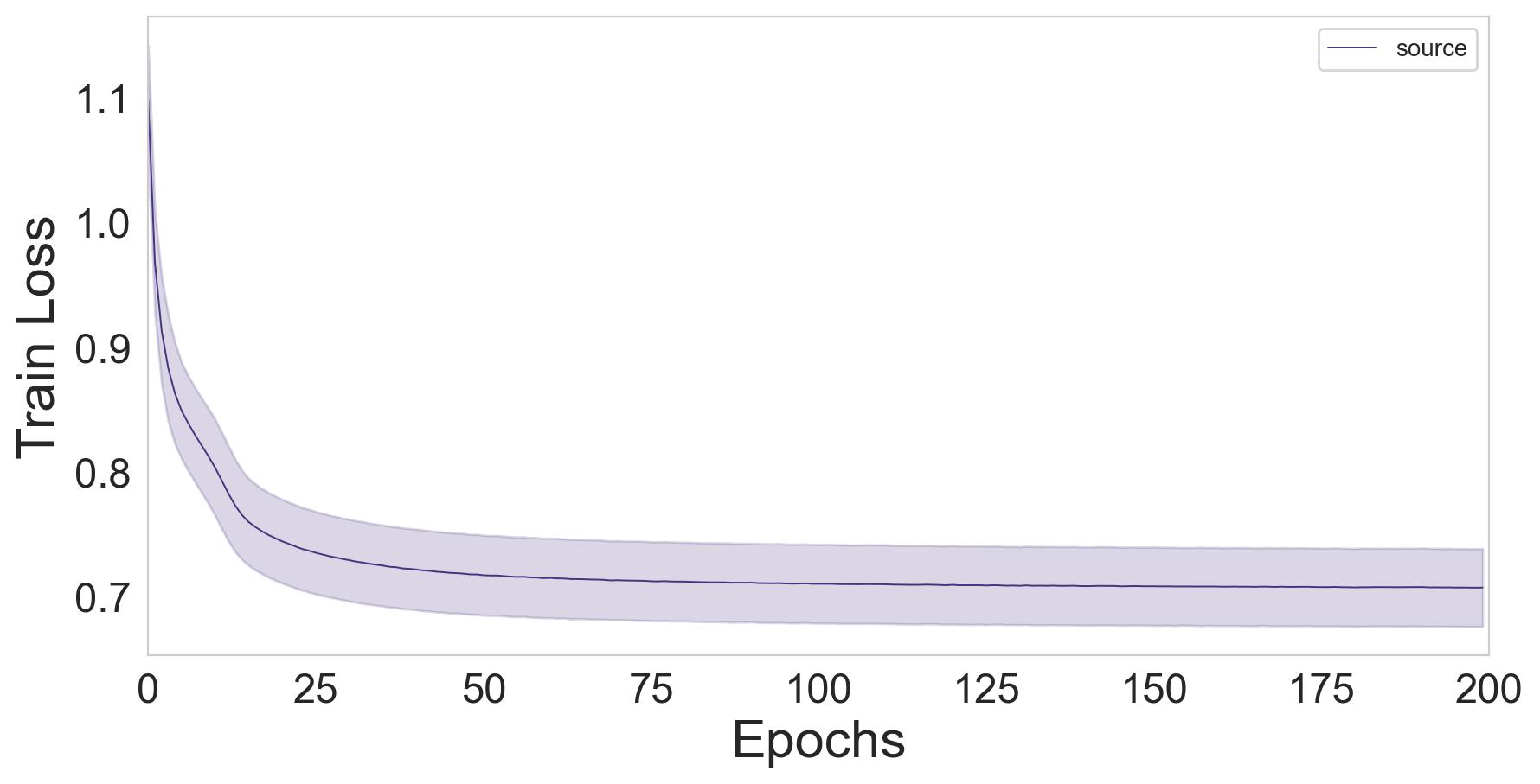
(a) Linear subspace data with 5% noisy samples and SNR = 20 [dB].

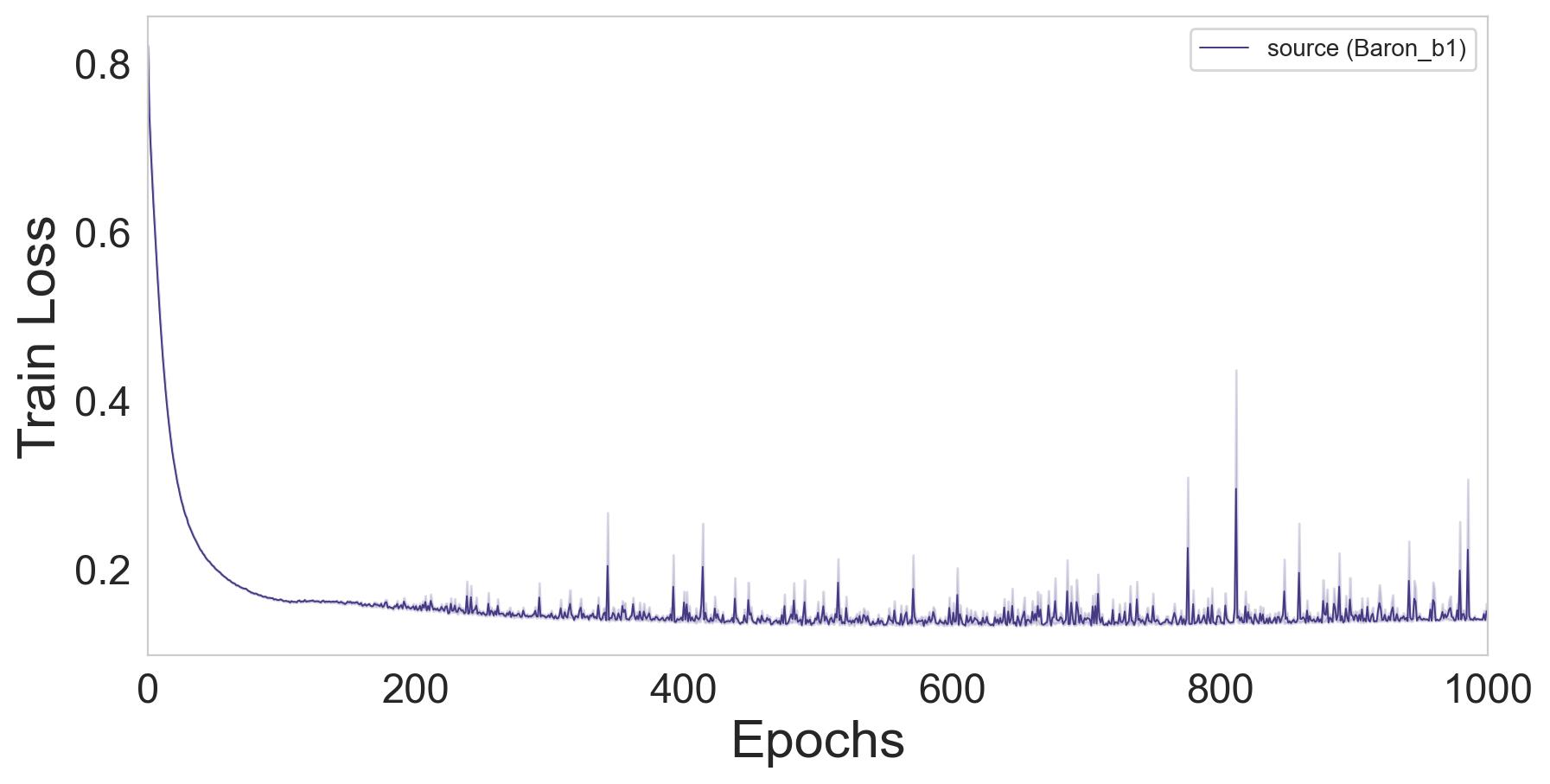
(b) Single-cell RNA data trained on the ’Baron’ batch.

Figure 32: Epoch-wise train loss influenced by the amount of domain shift.

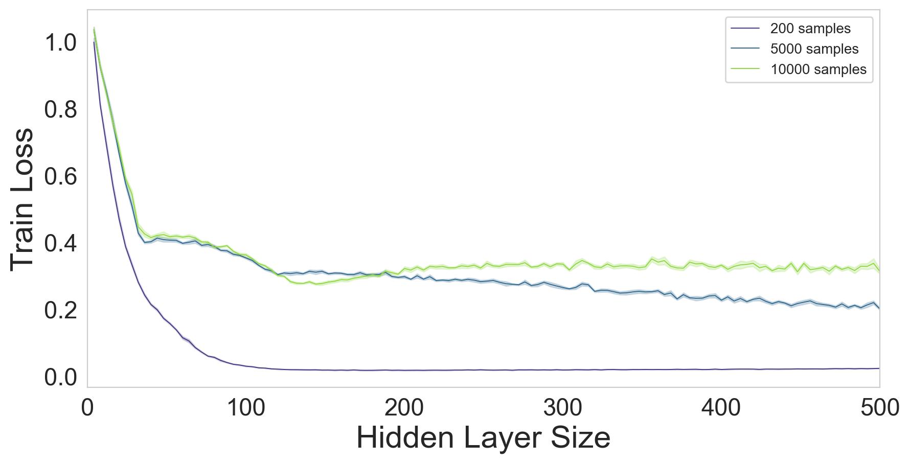
Figure 33: Train loss of the linear subspace data with sample noise = 70% and SNR = -15 [dB] for different number of training samples.

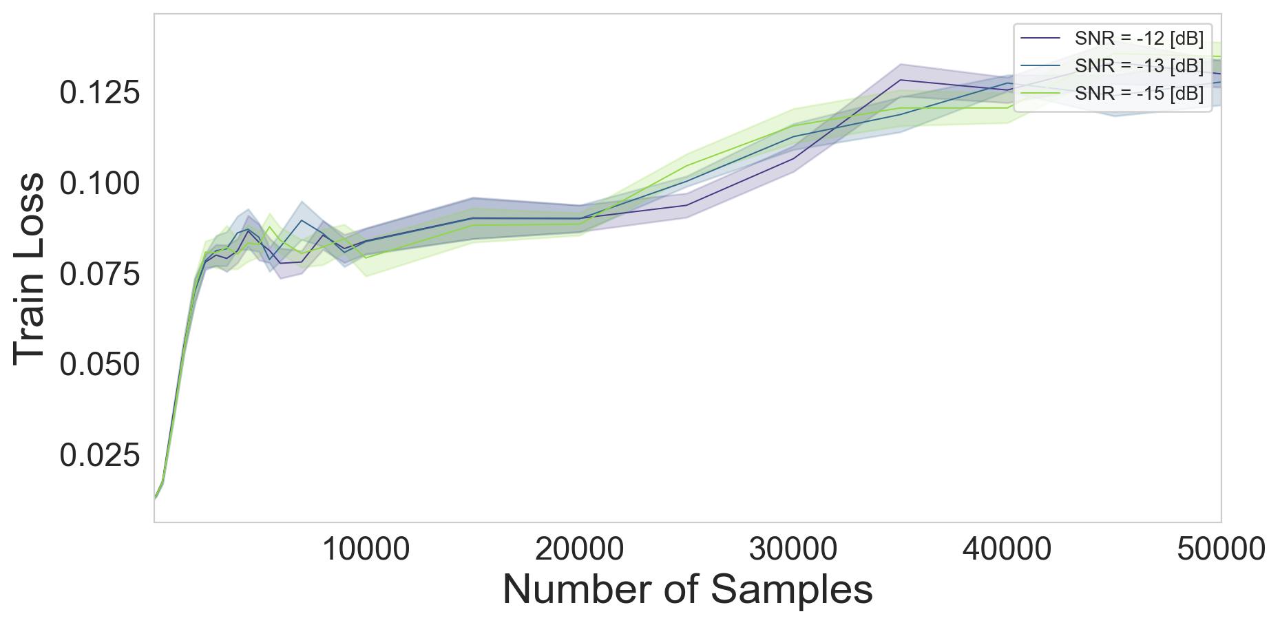
(a) sample noise = 90%.

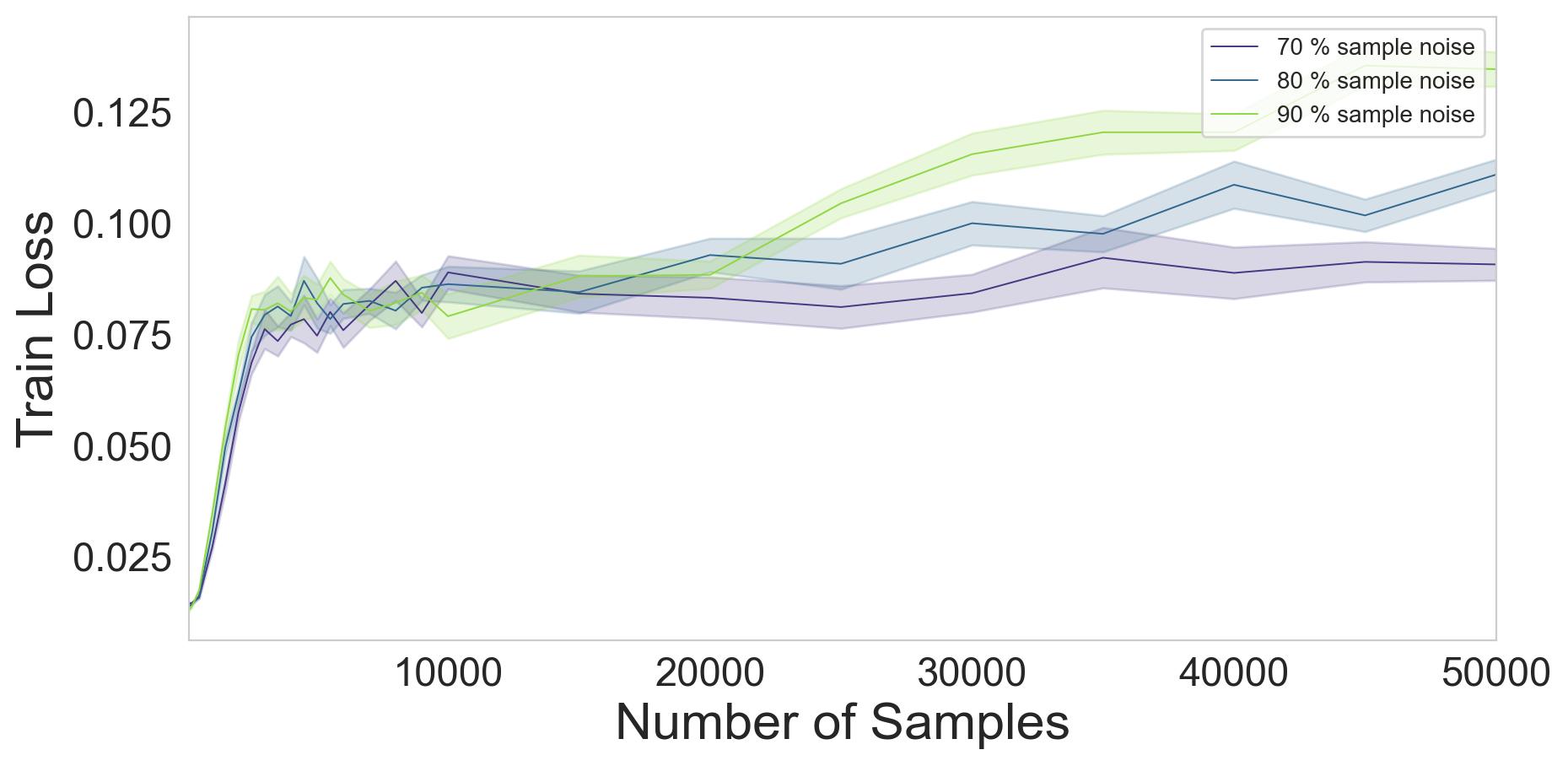
(b) Sample noise scenario. SNR = -15 [dB].

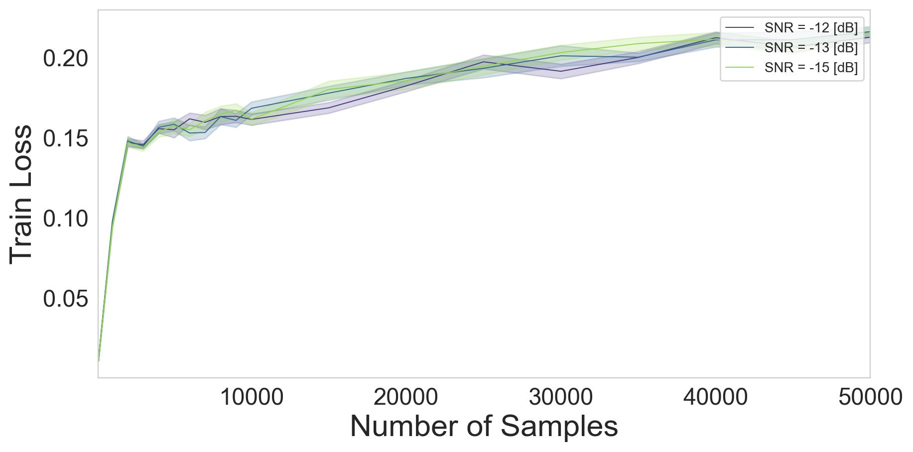
(c) Feature noise = 90 %.

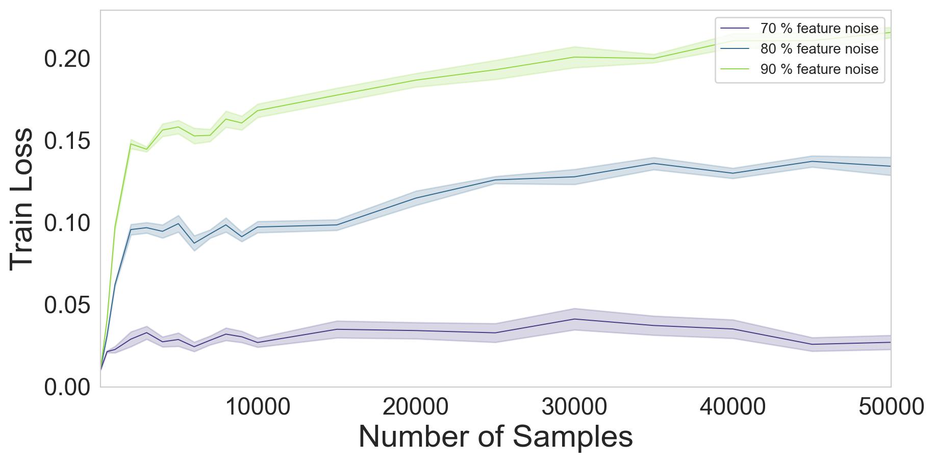
(d) Feature noise scenario. SNR = -13 [dB].

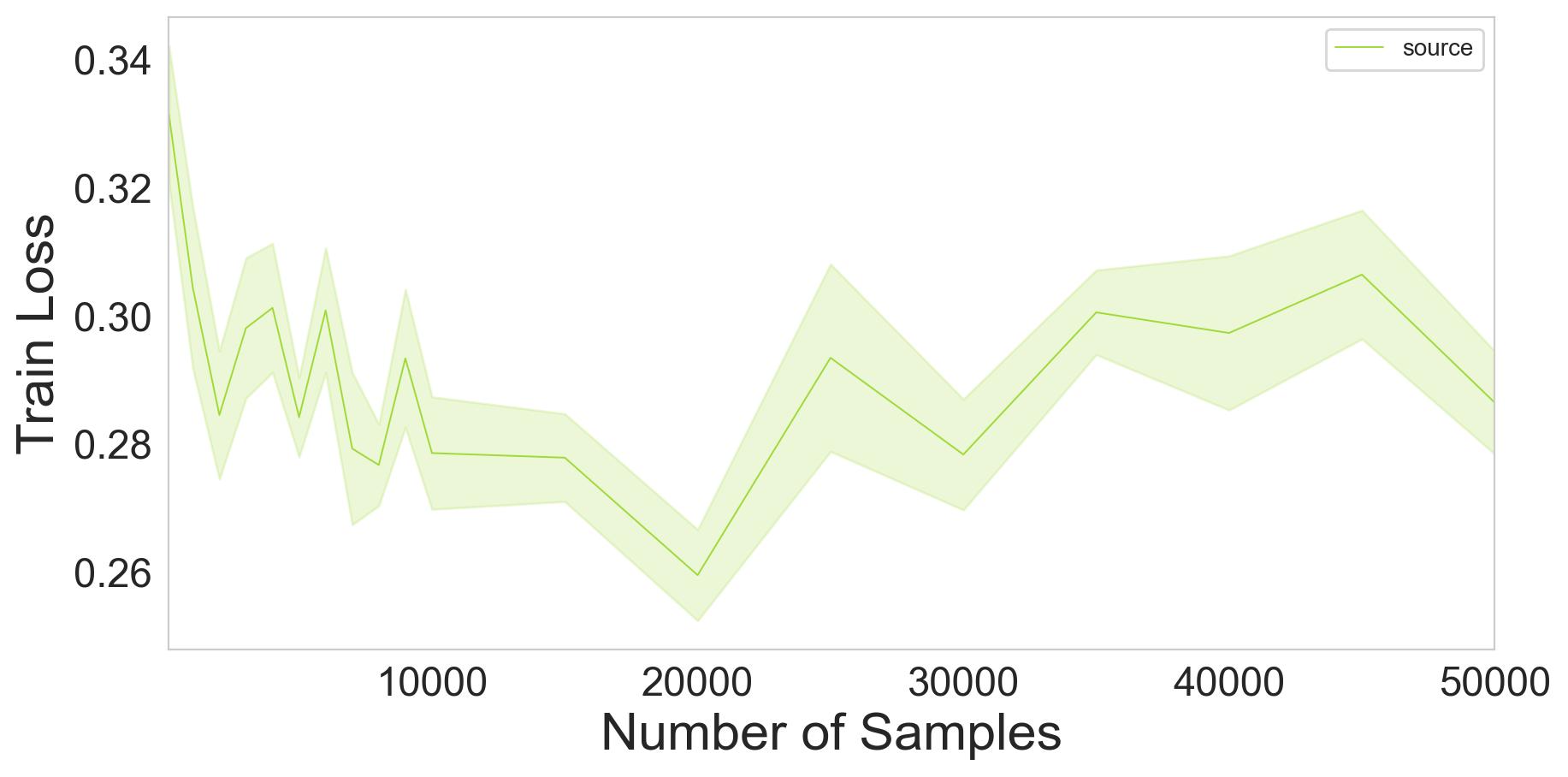
(e) Domain shift scenario.

Figure 34: Train losses rise as the number of samples increase. The rise occurs due to the model entering the under-parameterized regime for larger number of training samples. However, despite the increase in training loss with a higher number of samples, the test loss decreases, suggesting improved reconstruction of the test samples.

Appendix D More Results For Domain Adaptation

This section presents the domain adaptation results for the linear subspace dataset. UMAP visualization of the different domains is illustrated in Figure 35 and results for different model sizes are reported in Figure 36.

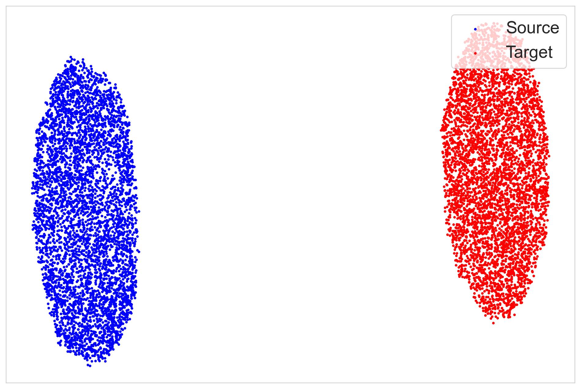
Figure 35: The UMAP representation shows a clear domain shift between the source and target datasets, as there is no overlap between the two clusters.

Figure 36 illustrates the results based on a similar experiment conducted in Section 5.1 for the case of linear subspace data. As expected, the interpolating models exhibit the poorest KNN-DAT outcomes. Over-parameterized models introduce a decrease in the test loss indicating an improved reconstruction of the target data. In this scenario, we noticed that smaller models perform better than over-parameterized models based on KNN-DAT results. We think that the small size of the hidden layer (4) and the high dimensionality of the dataset (50 features) result in significant information loss in these layers. This could lead to closely clustered vectors in the embedding space, ultimately causing low KNN-DAT results. However, the high training loss for a hidden layer of size 4 indicates insufficient capacity to represent the signal, as shown by the high values of test and train losses in Figure 36.

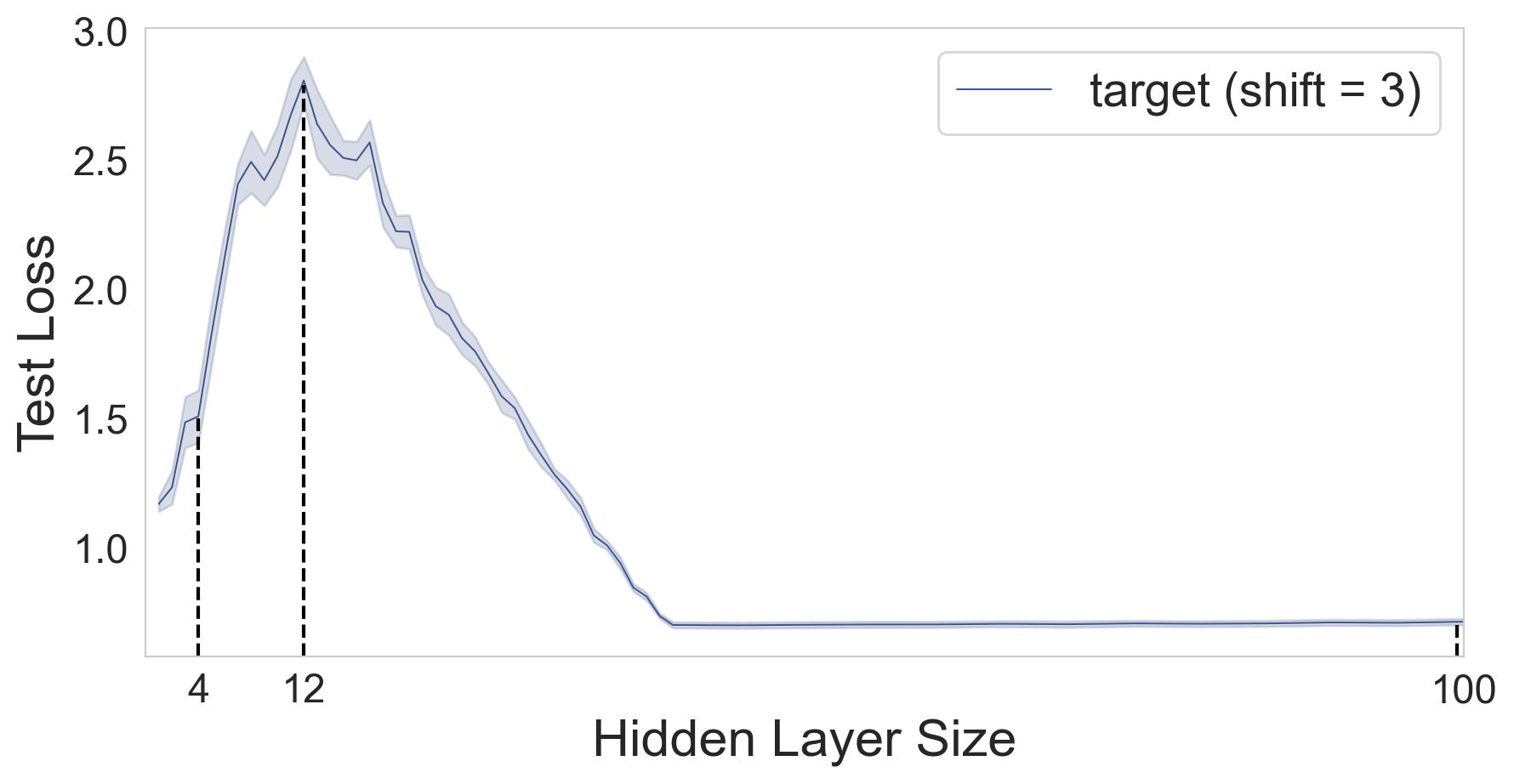
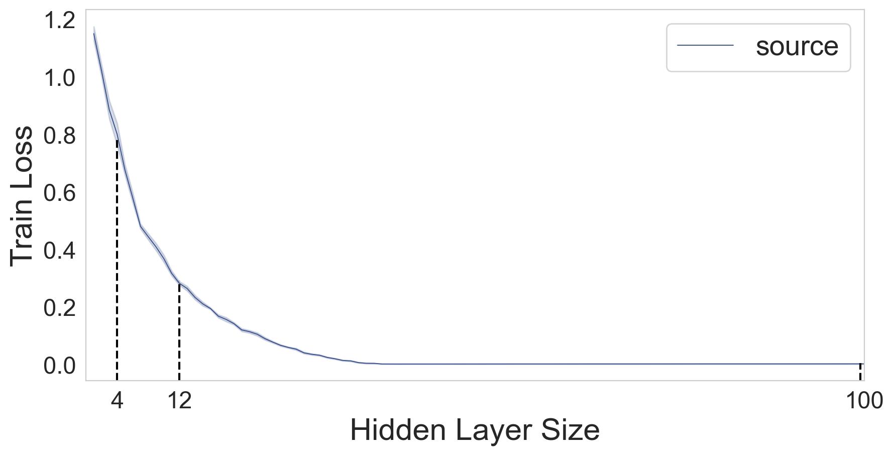
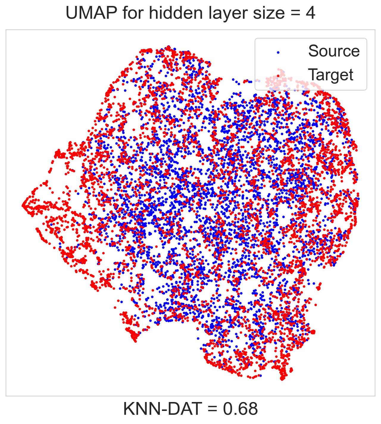
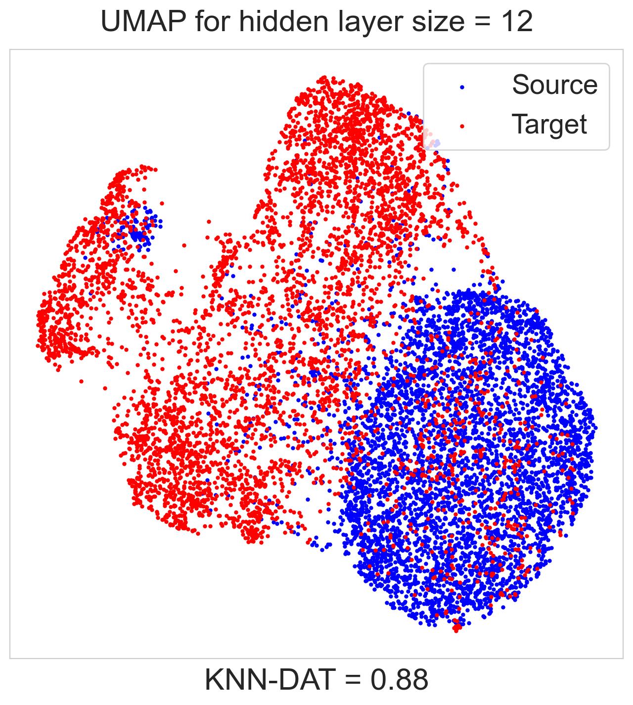
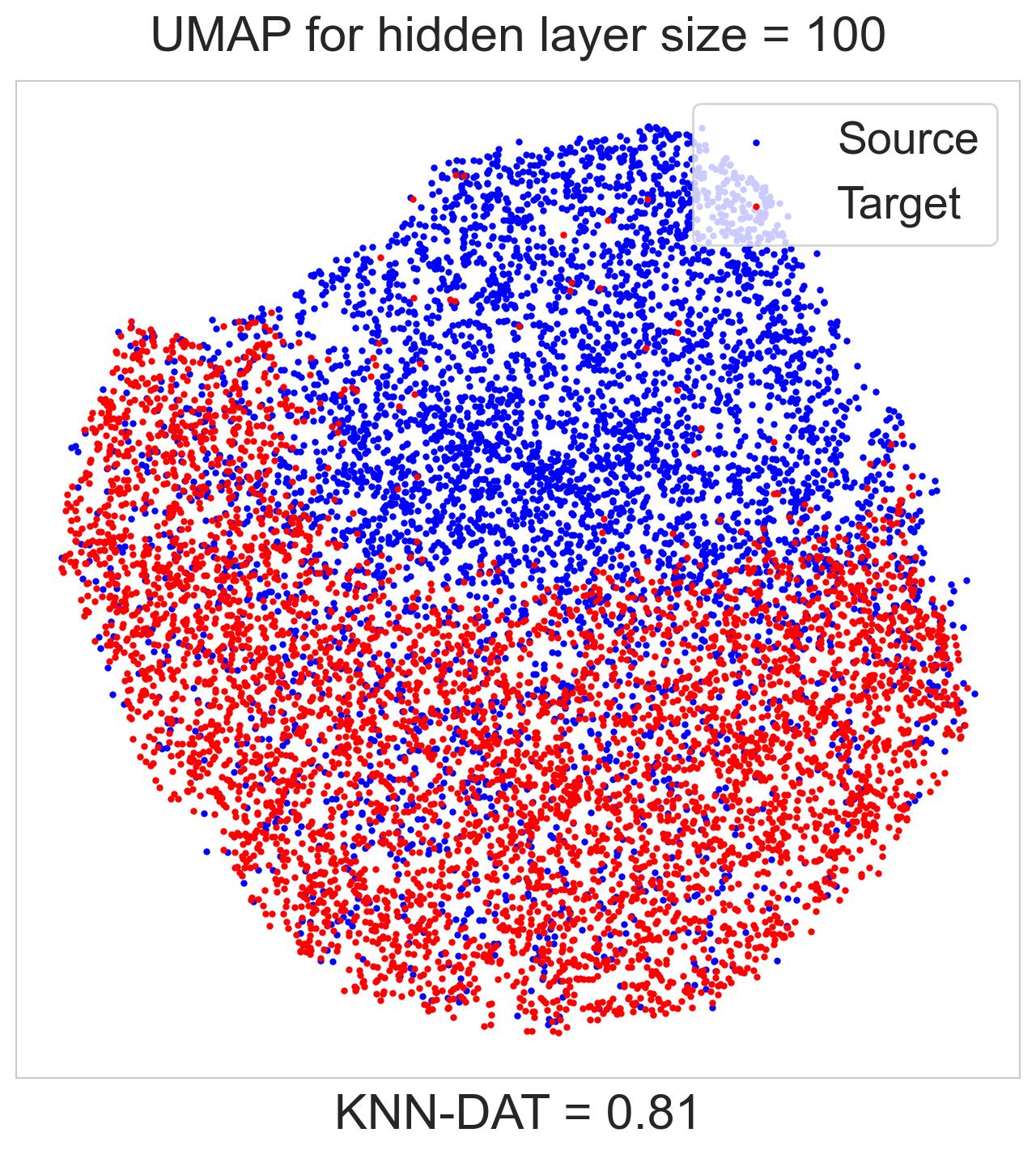
Figure 36: UMAP of the latent (bottleneck) vectors with a size of 45 and KNN-DAT results for different model sizes trained on the linear subspace dataset for a shift of 3.

References

- [1] Trevor Hastie, Robert Tibshirani, Jerome H Friedman, and Jerome H Friedman. The elements of statistical learning: data mining, inference, and prediction, volume 2. Springer, 2009.
- [2] Alex Krizhevsky, Ilya Sutskever, and Geoffrey E Hinton. Imagenet classification with deep convolutional neural networks. Advances in neural information processing systems, 25, 2012.
- [3] Kaiming He, Xiangyu Zhang, Shaoqing Ren, and Jian Sun. Deep residual learning for image recognition. In Proceedings of the IEEE conference on computer vision and pattern recognition, pages 770–778, 2016.
- [4] Chiyuan Zhang, Samy Bengio, Moritz Hardt, Benjamin Recht, and Oriol Vinyals. Understanding deep learning (still) requires rethinking generalization. Communications of the ACM, 64(3):107–115, 2021.
- [5] Madhu S Advani, Andrew M Saxe, and Haim Sompolinsky. High-dimensional dynamics of generalization error in neural networks. Neural Networks, 132:428–446, 2020.
- [6] Behnam Neyshabur, Zhiyuan Li, Srinadh Bhojanapalli, Yann LeCun, and Nathan Srebro. Towards understanding the role of over-parametrization in generalization of neural networks. arXiv preprint arXiv:1805.12076, 2018.
- [7] Mikhail Belkin, Alexander Rakhlin, and Alexandre B Tsybakov. Does data interpolation contradict statistical optimality? In The 22nd International Conference on Artificial Intelligence and Statistics, pages 1611–1619. PMLR, 2019.
- [8] Mikhail Belkin, Daniel J Hsu, and Partha Mitra. Overfitting or perfect fitting? risk bounds for classification and regression rules that interpolate. Advances in neural information processing systems, 31, 2018.
- [9] Mikhail Belkin, Daniel Hsu, Siyuan Ma, and Soumik Mandal. Reconciling modern machine-learning practice and the classical bias–variance trade-off. Proceedings of the National Academy of Sciences, 116(32):15849–15854, 2019.
- [10] Preetum Nakkiran, Gal Kaplun, Yamini Bansal, Tristan Yang, Boaz Barak, and Ilya Sutskever. Deep double descent: Where bigger models and more data hurt. Journal of Statistical Mechanics: Theory and Experiment, 2021(12):124003, 2021.
- [11] Yehuda Dar, Vidya Muthukumar, and Richard G Baraniuk. A farewell to the bias-variance tradeoff? an overview of the theory of overparameterized machine learning. arXiv preprint arXiv:2109.02355, 2021.
- [12] Stefano Spigler, Mario Geiger, Stéphane d’Ascoli, Levent Sagun, Giulio Biroli, and Matthieu Wyart. A jamming transition from under-to over-parametrization affects loss landscape and generalization. arXiv preprint arXiv:1810.09665, 2018.
- [13] Matteo Gamba, Erik Englesson, Mårten Björkman, and Hossein Azizpour. Deep double descent via smooth interpolation. arXiv preprint arXiv:2209.10080, 2022.
- [14] Ben Adlam and Jeffrey Pennington. The neural tangent kernel in high dimensions: Triple descent and a multi-scale theory of generalization. In International Conference on Machine Learning, pages 74–84. PMLR, 2020.
- [15] Tengyuan Liang, Alexander Rakhlin, and Xiyu Zhai. On the multiple descent of minimum-norm interpolants and restricted lower isometry of kernels. In Conference on Learning Theory, pages 2683–2711. PMLR, 2020.
- [16] Lin Chen, Yifei Min, Mikhail Belkin, and Amin Karbasi. Multiple descent: Design your own generalization curve. Advances in Neural Information Processing Systems, 34:8898–8912, 2021.
- [17] Stéphane d’Ascoli, Levent Sagun, and Giulio Biroli. Triple descent and the two kinds of overfitting: Where & why do they appear? Advances in Neural Information Processing Systems, 33:3058–3069, 2020.
- [18] Lorenzo Luzi, Yehuda Dar, and Richard Baraniuk. Double descent and other interpolation phenomena in gans. arXiv preprint arXiv:2106.04003, 2021.
- [19] Chengyu Dong, Liyuan Liu, and Jingbo Shang. Double descent in adversarial training: An implicit label noise perspective. 2021.
- [20] Mengzhou Xia, Mikel Artetxe, Chunting Zhou, Xi Victoria Lin, Ramakanth Pasunuru, Danqi Chen, Luke Zettlemoyer, and Ves Stoyanov. Training trajectories of language models across scales. arXiv preprint arXiv:2212.09803, 2022.
- [21] Peter L Bartlett, Philip M Long, Gábor Lugosi, and Alexander Tsigler. Benign overfitting in linear regression. Proceedings of the National Academy of Sciences, 117(48):30063–30070, 2020.
- [22] Zhu Li, Weijie Su, and Dino Sejdinovic. Benign overfitting and noisy features. arXiv preprint arXiv:2008.02901, 2020.
- [23] Jonathon Shlens. A tutorial on principal component analysis. arXiv preprint arXiv:1404.1100, 2014.
- [24] William F Massy. Principal components regression in exploratory statistical research. Journal of the American Statistical Association, 60(309):234–256, 1965.
- [25] Daniel Gedon, Antônio H Ribeiro, and Thomas B Schön. No double descent in pca: Training and pre-training in high dimensions. 2022.
- [26] Ji Xu and Daniel J Hsu. On the number of variables to use in principal component regression. Advances in neural information processing systems, 32, 2019.
- [27] Ningyuan Teresa, David W Hogg, and Soledad Villar. Dimensionality reduction, regularization, and generalization in overparameterized regressions. SIAM Journal on Mathematics of Data Science, 4(1):126–152, 2022.
- [28] Alisia Lupidi, Yonatan Gideoni, and Dulhan Jayalath. Does double descent occur in self-supervised learning? arXiv preprint arXiv:2307.07872, 2023.
- [29] Rishi Sonthalia and Raj Rao Nadakuditi. Training data size induced double descent for denoising feedforward neural networks and the role of training noise. Transactions on Machine Learning Research, 2023.
- [30] Marina Dubova. Generalizing with overly complex representations. In NeurIPS 2022 Workshop on Information-Theoretic Principles in Cognitive Systems, 2022.
- [31] Zhengming Zhang, Taotao Ji, Haoqing Shi, Chunguo Li, Yongming Huang, and Luxi Yang. A self-supervised learning-based channel estimation for irs-aided communication without ground truth. IEEE Transactions on Wireless Communications, 2023.
- [32] Hoa Thi Nhu Tran, Kok Siong Ang, Marion Chevrier, Xiaomeng Zhang, Nicole Yee Shin Lee, Michelle Goh, and Jinmiao Chen. A benchmark of batch-effect correction methods for single-cell rna sequencing data. Genome biology, 21:1–32, 2020.
- [33] Kaiyang Zhou, Ziwei Liu, Yu Qiao, Tao Xiang, and Chen Change Loy. Domain generalization: A survey. IEEE Transactions on Pattern Analysis and Machine Intelligence, 45(4):4396–4415, 2022.
- [34] Xingchao Peng, Qinxun Bai, Xide Xia, Zijun Huang, Kate Saenko, and Bo Wang. Moment matching for multi-source domain adaptation. In Proceedings of the IEEE/CVF international conference on computer vision, pages 1406–1415, 2019.
- [35] Woong-Gi Chang, Tackgeun You, Seonguk Seo, Suha Kwak, and Bohyung Han. Domain-specific batch normalization for unsupervised domain adaptation. In Proceedings of the IEEE/CVF conference on Computer Vision and Pattern Recognition, pages 7354–7362, 2019.
- [36] Amit Rozner, Barak Battash, Lior Wolf, and Ofir Lindenbaum. Domain-generalizable multiple-domain clustering. Transactions on Machine Learning Research, 2023.
- [37] Tamir Baruch Yampolsky, Ronen Talmon, and Ofir Lindenbaum. Domain and modality adaptation using multi-kernel matching. In 2023 31st European Signal Processing Conference (EUSIPCO), pages 1285–1289. IEEE, 2023.
- [38] Leland McInnes, John Healy, and James Melville. Umap: Uniform manifold approximation and projection for dimension reduction. arXiv preprint arXiv:1802.03426, 2018.
- [39] Mark F Schilling. Multivariate two-sample tests based on nearest neighbors. Journal of the American Statistical Association, 81(395):799–806, 1986.
- [40] Varun Chandola, Arindam Banerjee, and Vipin Kumar. Anomaly detection: A survey. ACM computing surveys (CSUR), 41(3):1–58, 2009.
- [41] Ofir Lindenbaum, Yariv Aizenbud, and Yuval Kluger. Probabilistic robust autoencoders for outlier detection. The Conference on Uncertainty in Artificial Intelligence (UAI), 2024.
- [42] Zhaomin Chen, Chai Kiat Yeo, Bu Sung Lee, and Chiew Tong Lau. Autoencoder-based network anomaly detection. In 2018 Wireless telecommunications symposium (WTS), pages 1–5. IEEE, 2018.
- [43] Amit Rozner, Barak Battash, Henry Li, Lior Wolf, and Ofir Lindenbaum. Anomaly detection with variance stabilized density estimation. The Conference on Uncertainty in Artificial Intelligence (UAI), 2024.
- [44] Songqiao Han, Xiyang Hu, Hailiang Huang, Minqi Jiang, and Yue Zhao. Adbench: Anomaly detection benchmark. Advances in Neural Information Processing Systems, 35:32142–32159, 2022.
- [45] Diederik P Kingma and Jimmy Ba. Adam: A method for stochastic optimization. arXiv preprint arXiv:1412.6980, 2014.