Modified homotopy approach for diffractive production in the saturation region
Carlos Contreras
carlos.contreras@usm.clDepartamento de Física, Universidad Técnica Federico Santa María, Avda. España 1680, Casilla 110-V, Valparaíso, Chile
José Garrido
jose.garridom@usmcl.onmicrosoft.comDepartamento de Física, Universidad Técnica Federico Santa María, Avda. España 1680, Casilla 110-V, Valparaíso, Chile
Eugene Levin
leving@tauex.tau.ac.ilDepartment of Particle Physics, School of Physics and Astronomy,
Raymond and Beverly Sackler
Faculty of Exact Science, Tel Aviv University, Tel Aviv, 69978, Israel
Rodrigo Meneses
rodrigo.meneses@uv.clEscuela de Ingeniería Civil, Facultad de Ingeniería, Universidad de Valparaíso,Avda General Cruz 222 , Valparaíso, Chile
Abstract
In this paper we continue to develop the homotopy method for solving of the non linear evolution equation for the diffractive production in deep inelastic scattering(DIS). We introduce part of the nonlinear corrections as a first step of this approach. This simplified nonlinear evolution equation is solved analytically taking into account the initial and boundary conditions for the process. At the second step of our approach we demonstrated that
the perturbative procedure can be used for the remaining parts of the non-linear corrections. It turns out that these corrections are small and can be estimated in the regular iterative procedure.
pacs:
12.38.Cy, 12.38g,24.85.+p,25.30.Hm
I Introduction
In this paper we continue our search for the regular iteration procedure of solving non-linear equations that in QCD governs dynamics in the saturation region. In our previous paperCLMNEW we developed the homotopy solution HE1 ; HE2 for the Balitsky-Kovchegov (BK) equationBK that give the dipole scattering amplitude. It has been shown that this approach allows us to collect all essential contribution into the linear equation which can be solved analytically, and to propose the iteration procedure, which is being partly numerical, leads to small corrections. In this paper our main goal is to expand this approach to the processes of diffraction production in deep inelastic scattering (DIS).
The non-linear evolution equation that describes these processes have been derived in Ref.KOLE (see also HWS ; HIMST ; KLW ; KLP .The close attention of the high energy community to these processes KOLE ; HWS ; HIMST ; KLW ; KLP ; LEWU ; GBKW ; GOLEDD ; SATMOD0 ; KOML ; MUSCH ; MASC ; MAR ; KLMV ; LELUDD ; LELUDD1 ; KOLEB ; CLMP ; CLMP1 ; MM1 ; MM2 ; MM3 shows the need to find effective procedure for solving the equations.
In derivation of the non-linear equations two approaches are used: the unitarity constraints for the dipoles scattering amplitude and the AGKAGK cutting rules. In
Ref.KLP has been shown that this non-linear evolution has the same structure for all in DIS, where is the cross section of the produced -dipoles in the final state. Therefore, we view this paper as a starting point for finding for DIS.
Diffractively we produces the system of dipoles with low multiplicities and the large rapidity gap between them and recoiled target. The total cross section of diffractive production can be viewed as : production of particles with multiplicities lower that the average one.
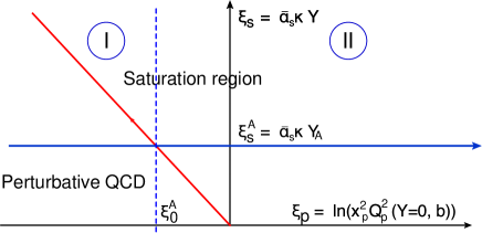
Figure 1: Saturation region of QCD for the elastic scattering amplitude. The critical line (z=0) is shown in red. The initial condition for scattering with the dilute system of partons (with proton) is given at . For heavy nuclei the initial conditions are placed at , where is the number of nucleon in a nucleus. The line, where they are given, is shown in blue.
The homotopy method we can use for the general equation:
(I.1)
where the linear part is a differential or integral-differential operator, but non-linear part has an arbitrary form. As a solution, we introduce the following equation for the homotopy function :
with . Eq. (I.3) gives the solution to the non-linear equation at . The hope is that several terms in series of Eq. (I.3) will give a good approximation in the solution of the non-linear equation.
The linear equation is obvious in the perturbative QCD region (see Fig. 1, where it is the BFKL equation BFKL ; LIP ; LIREV . However, in Ref.CLMNEW we showed that inside the saturation region (see Fig. 1) we can find the linearized equation based on the approach of Ref.LETU . In this paper we include in part of the non-linear corrections which can be treated analytically.
We demonstrate that non-linear terms which include the remains of the non-linear corrections, lead to small contributions and can be treated in perturbation approach.
The detailed description of our approach is included in the next section. Here we wish
to discuss the kinematic region where we are looking for the solution and general assumptions that we make in fixing initial and boundary conditions. In Fig. 1 the main kinematic regions are shown for the scattering amplitude of a dipole () with a nucleus target in the plot with and axes, where
and
The saturation moment is equal to
(I.4)
where are determined by the following equations111 is the BFKL kernelBFKL in anomalous dimension () representation. .
:
(I.5)
In Fig. 1 one can see that for we have
the perturbative QCD region where the non-linear corrections are small and we can safely use the BFKL linear equation for the scattering amplitude. is defined as follows
(I.6)
with .
In Eq. (I.6) and Eq. (I.4) denotes , where is the number of nucleons in a nucleus.
For the non-linear corrections become essential and we enter the saturation region. For the scattering with nuclei, which we consider in this paper, the saturation region can be divided in two parts. For the amplitude has the geometric scaling behaviour BALE ; GS and it depends only on one variable . For
this geometric scaling behaviour is broken.
For diffractive production we have more complex kinematics (see Fig. 2 for the diffraction production in the region of small mass). From this figure one can see that we have several different kinematic regions for where
(I.7)
is the cross section of diffractive production with the rapidity gap larger than )(see Fig. 2).
This process can be characterized by two saturation momentums: and . For and we can replace in Fig. 2-b by the BFKL Pomeron and the diffraction cross section can be calculated using triple Pomeron diagram.
For and we have the situation which is shown in Fig. 2. The elastic amplitude is in the saturation region and the production of gluons can be computed using the BFKL Pomeron exchange.
Finally, for and
the large mass is produced and is the kinematic region where non-linear corrections for gluon production are essential. The main goal of this paper is to find reliable procedure to calculate in this kinematic region.
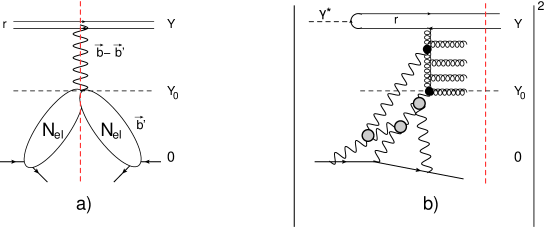
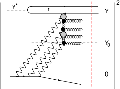
Figure 2: The graphic representation of the processes of
diffraction production. Fig. 2-a shows the first Mueller diagram MUDI for the diffractive production in the scattering of one dipole with size and rapidity . In this diagram we indicate the impact parameters and which we used in the text. The wavy lines denote the BFKL Pomeron. The vertical dashed line shows that all gluons of this Pomeron are produced. Fig. 2-b shows the general structure of the diagrams that has been taken into account in the equation of Ref. KOLE . In this figure we clarify the notation for the rapidity gap and the rapidity region which is filled by produced gluons.
We have to specify the region of which we are dealing with in the saturation region . As has been noted in
Refs.GOST ; BEST actually for very large the non-linear corrections are not important and we have to solve linear BFKL equation. This feature can be seen directly
from the eigenfunction of this equation. Indeed, the eigenfunction
(the scattering amplitude of two dipoles with sizes and ) has the
following form LIP
(I.8)
One can see that for , starts to be smaller and the non-linear term in the BK equation
could be neglected. In this paper we consider the interaction with the nucleus and the scattering amplitude of the dipole with a nucleus for the exchange of the BFKL Pomeron has the following form:
(I.9)
where is the size of a nucleon, is the impact parameter for dipole-nucleon amplitude and is the position of the nucleon with respect to the center of the nucleus. is the number of nucleons in a nucleus. Since we can integrate over replacing by and obtain the expression:
(I.10)
Therefore, in this case we can absorb all dependence on the impact parameter in the dependence of the saturation scale. In Eq. (I.10) we implicitly assume that .
The typical process, that we bear in mind, is the deep inelastic scattering(DIS) with a nucleus at and at small values of .
In this equation is the imaginary part of the elastic scattering amplitude of the dipole with the size and rapidity at the impact parameter (see Fig. 2). is the cross section of the diffractive production with the rapidity gap larger than for the same scattering process. The cross section of the diffractive production of particles (gluons) in rapidity region (, see Fig. 3) can be found from the following equation
(II.2)
From Eq. (II.2) one can see that Eq. (II.1) gives :
(II.3)
where , and is the obvious shorthand for , and respectively. In Fig. 3 we pictured each of the contribution in Eq. (II.1) and Eq. (II.3).
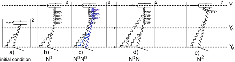
Figure 3: The graphic representation of the terms of Eq. (II.1) for
diffraction production. Fig. 3-a shows the initial conditions for .
Fig. 3-b is the linear equation for , while Fig. 3-c describes the non-linear contribution . Fig. 3-d shows the shadowing correction due to enhanced diagrams. The wavy lines denote the BFKL Pomeron while the helix ones describe the gluons.
For large the elastic amplitude is in the saturation region and close to 1. Replacing and neglecting term for
(see Fig. 3-c) one can see that Eq. (II.3) reduces to the linear equation
where is the saturation momentum. It is well known that to find the saturation momentum we need to consider the linear equation, which correspond to Fig. 3-b. It can be written as (see Eq. (I.8) and Ref.CLMS )
(II.6)
Taking this integral using the method of steepest decent (see Refs.GLR ; MUT ) we obtain that . We need to take integral over in Eq. (II.6) to find the typical values of . First one can see that integral over (see Eq. (I.8)) leads to extra factor since . Finally,
the integral over has a form:
(II.7)
since for .
Bearing this in mind integral in Eq. (II.5) gives :
(II.8)
Introducing of Eq. (I.6) one can see that .
From Eq. (II.4) we can conclude that decreases with .
It turns out that Eq. (II.1) can be rewritten in this simple form,
introducing a new function:
(II.9)
where is the solution to the BK equation and is given by Eq. (I.6). The new variables and are defined as and .
This function has a clear meaning: the inelastic cross section of all events with the rapidity gap from to .
For function Eq. (II.1) takes the form of the BK equation, viz.:
(II.10)
The initial conditions for this equation is the following:
where is a smooth function of . However, Eq. (II.13) only holds in region I in Fig. 1, while in region II we have to use a more general expressions for the elastic scattering amplitudes (see Ref.CLMNEW ). We will discuss the initial condition in this region below.
Our strategy of finding this solution looks as follows: first we are going to solve Eq. (II.10) and find , and after that we will return to Eq. (II.1).
III Modified homotopy approach for
III.1 Generalities
As previously mentioned we use the homotopy approach to find the solution to non-linear equation of Eq. (II.10), suggested in Refs.HE1 ; HE2 ; CLMNEW .
In this paper we modify the homotopy approach by including the part of the non-linear term into definition of .
Following the main ideas of Ref.LETU we solve Eq. (II.10) replacing by . For this function the equation takes the form:
(III.1)
and the initial conditions for takes the following formCLMS :
(III.2a)
(III.2b)
with
(III.2c)
where is defined as and .
We suggest to simplify the non-linear term replacing it with
(III.3)
with which is determined by Eq. (I.6) by replacing by . This contribution stems from the region (see Ref.LETU ) and
we believe that Eq. (III.3) is a good approximation for the integral. W]e can treat the corrections to this equation in a perturbation approach.
We modify the homotopy approach :
taking
(III.4)
we find the solution to the equation:
(III.5)
It turns out that searching for the function it is more transparent to
return to Eq. (II.10), which can be rewritten in the region where or in the form (see Ref.LETU and section II-C-2 of Ref.CLMS ):
(III.6)
Introducing we obtain:
(III.7)
III.2 Solutions to the master equation
III.2.1 Geometric scaling solution to the master equation
Searching for the function we can rewrite Eq. (III.7) in the form222It is worthwhile mentioning that this solution
give the violation of the geometric scaling behaviour of the scattering amplitude due to dependence of on and .:
where is a constant. Integrating Eq. (III.10) we have
(III.11)
Constant as well as can be found from the solution of the linear equation. Assuming that is large we can neglect the contribution of in Eq. (III.11). Solution in this kinematics we know (see Refs.CLMP ; CLMP1 ):
This equation has
the traveling wave solution (see 3.4.1.1 of Ref.MATH2 :
(III.17)
Eq. (III.17) can be rewritten as follows333 In Eq. (III.18) the parameters , , and are redefined in comparison with Eq. (III.17) but we keep the same notations for simplicity.
but of to satisfy the initial condition of Eq. (III.2b):
(III.18)
where and
(III.19)
Indeed, for and we can neglect in Eq. (III.18) and this equation gives
(III.20)
one can see that is not determined by the initial condition and it has to be found from the boundary conditions on the line .
III.3 Initial and boundary conditions
III.3.1 Region I
We have found (seeEq. (III.11) ) which satisfies the boundary conditions of Eq. (III.2a).
The implicit relation of Eq. (III.11) for can be resolved for large . Indeed, expanding
We rewrite as
(III.22)
Plugging Eq. (III.3.1) in Eq. (III.22) for function we obtain:
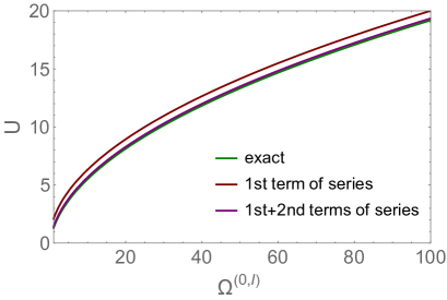
(III.23)
Eq. (III.23) gives the series representation of function . Fig. 4 shows that this series approximate quite well even if we restrict ourselves by first two terms. Actually, one can see from Fig. 4 that at large the first term in Eq. (III.23) approximates the exact solution quite well.
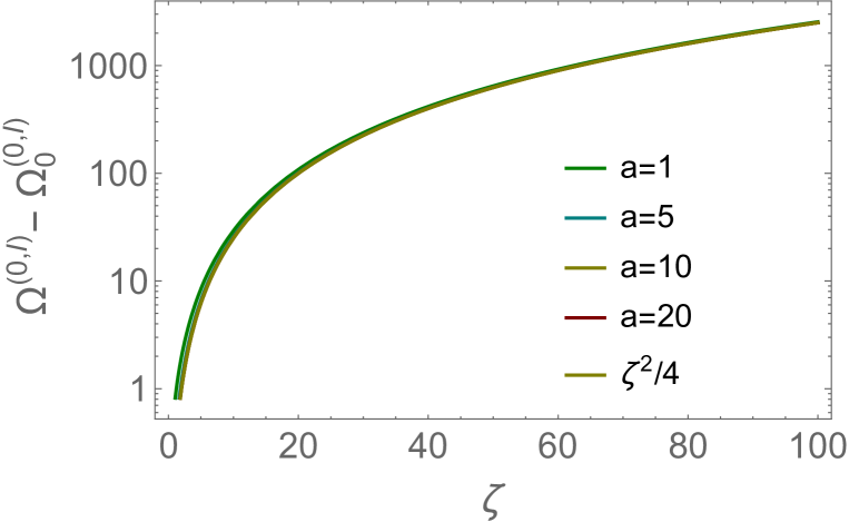
Figure 5: Function from Eq. (III.27) versus
for different values of .
In Fig. 5 we plot versus , where is given by Eq. (III.22). One can see that the first iteration of Eq. (III.26) describes the exact evaluation quite well.
III.3.2 Region II
One can see from Eq. (III.22) and Eq. (III.18) that is the solution of the equation:
(III.28)
where and is the same function that we have discussed in the previous section but with different values of the parameter (see Eq. (III.19)). The value of (see Eq. (III.19) is large and therefore we can use Eq. (III.25) which takes the form:
(III.29)
or for we have
(III.30)
where
(III.31)
It is instructive to find the solution restricting ourselves by the first term in the expansion of Eq. (III.30):
(III.32)
Recall, that has to be found from the boundary condition at .
III.3.3 Matching on the line
The value of parameter in Eq. (III.30) (see also Eq. (III.32)), can be found from the matching conditions on line or and has the following form:
(III.33)
where .
In the region I we use the approximate solution to Eq. (III.27) (see Fig. 5). is determined by Eq. (III.13). From Eq. (III.33) one can see that and
(III.34)
IV in modified homotopy approach
From Eq. (II.2) and Eq. (II.9) we can calculate which is equal to
(IV.1)
However, before making this evaluation we return to the master equation of Eq. (II.1) and rewrite it in the saturation region assuming , and . It takes the form
One can see that this is the same equation as for or for . Hence in the linear approximation we have in the region I:
(IV.4)
and in the region II:
(IV.5)
In general case we can use Eq. (IV.1) and calculate using Eq. (III.22) and Eq. (III.27). Indeed,
(IV.6)
Therefore,
(IV.7)
In the region I , while in the region II
and we need to replace by .
Actually, the same formula is correct for the elastic amplitude since Eq. (II.10) coincides with the BK equation BK . The only difference in the values of . In region I for the elastic amplitude is equal to
and in the region II .
V The second iteration for in the modified homotopy approach
In this section we return to the discussion of Eq. (III.3) for which we used a particular contribution. Now we are going to insert in this term and develop the second iteration of the master equation, choosing in the form
(V.1)
Let us estimate the first term in this equation plugging in solution at large , viz.:
(V.2)
Denoting by and introducing where is the projection on the direction of , we can rewrite the integral in the following form:
(V.3)
where and . In the region where these arguments are large we can use the method of steepest descent to take the integral. The equation for the saddle point are
(V.4a)
(V.4b)
One can see that Eq. (V.4a) does not have solution. It means that main contribution stems from which is the end point of the integral.
Eq. (V.4b) has the solution . So we can see two main contributions in the integral over : the end point of the integral: and the contribution of the saddle point. The first contribution has been taken into account in Eq. (III.3) and it has been subtracted in Eq. (V.1).
The estimates using the method of steepest descent has to be discussed calculating the second derivatives in the saddle point .
(V.5a)
(V.5b)
From
Eq. (V.5b) one can see that the saddle point approximation can be justified only in the limited region of : . For large the second derivatives is positive indicating that the integral has a minimum in this point. Integrating over we plot in Fig. 6 versus and different values of . One can see that at the integrant has a maximum at and can be taken using the method of steepest descent. However for this maximum disappears and only regions and contribute. These contributions have been taken into account in our first iteration. Hence we expect that the corrections from the second iteration can be small.
Figure 6: The ratio from Eq. (V.3) versus at different values of .
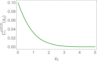
In Fig. 7 we present the numerical estimates for
of Eq. (I.1) :
(V.6)
One can see that for turns out to be small.
Figure 7: The ratio versus for . is taken to be 3.
V.1 Geometric scaling solution
The equation for the second iteration takes the form (see Eq. (I.2)):
(V.7)
Taking into account only terms of the order of , we have
(V.8)
The particular solution can be written as follows
(V.9)
As we have discussed (see Eq. (V.6)) we expect that will be small. Indeed, Fig. 8 shows that the ration turns out to be small.
Figure 8: The ratio versus for . is taken to be 3.
We need to add the general solution to the linear equation to satisfy the initial condition , which takes the form:
(V.10)
Hence the general form for is
(V.11)
Finding constant from Eq. (V.10) one can see that this constant turns out to be rather small, since turns put to be small at (In Fig. 8 at ).
V.2 Region II
In region II (see Fig. 1) the elastic scattering amplitude does not have the geometric scaling behaviour being the function of two variables: and . This function has been found in our previous paper CLMNEW
(see Eq.58 and Eq.67) and it has the form of Eq. (III.2c) for the initial conditions for . Bearing this in mind,
we choose in homotopy approach in the form of Eq. (III.4) in region II. The chosen gives
Eq. (V.1) for . For region II has the same form as of Eq. (V.1)
(V.12)
We need to investigate in the same way as we did in Eq. (V.1)-Eq. (V.3). For this analysis we take a simplified version of of Eq. (III.34) and Eq. (V.2). This version stems from the solution of the linear equation in which we neglect the non-linear terms in Eq. (III.5).
The solution to this linear equation is
(V.13)
Function has to be found from the initial condition of Eq. (III.2c), viz.:
Using Eq. (V.15) we are going to discuss the first term in Eq. (V.12).
From Eq. (V.13) and Eq. (V.15) we can conclude that the main contributions at large dipole sizes stem from the factor . This factor changes the behaviour of the integrant in Eq. (V.12) and the integral can be taken in the method of steepest descent at . In particular the contribution of the small size dipoles, that was essential in the region I , turns out to be small.
Let us demonstrate all of these features. First we rewrite the solution of Eq. (V.13) as follows:
(V.16)
plugging this equation in we have
(V.17)
where we denote , and . Introducing and we obtain:
(V.18)
One can see that the main contribution stems from since functions are logarithmic. Taking this integral for such we derive
(V.19)
with , , and .
The equation for the second iteration takes the form (see Eq. (I.2)):
(V.20)
Note, the two changes we make in Eq. (III.5): first, we use the variables and instead of and ; and second, we neglect the non-linear contributions by the same reason as in Eq. (V.8).
The particular solution to this equation has the form:
(V.21)
Finally, the solution which satisfies Eq. (V.10) has the following form:
(V.22)
Eq. (V.22) has the same qualitative features as in region I:
it vanishes at and in the region of large it approaches
with small constant .
VI Modified homotopy approach for in perturbative QCD region
In this section we consider the perturbative QCD (pQCD) region for the elastic amplitude. This region corresponds to the following kinematic restriction:
but . is so small that we can use in this region the BFKL Pomeron exchange for the scattering amplitude. First we consider the diagram of Fig. 3-b, the expression for which has been written in Eq. (II.6) with the only difference that is described by the exchange of the BFKL Pomeron, viz.:
(VI.1)
Assuming that we are in the vicinity of the saturation scale for the elastic amplitude, we see that Eq. (VI.1) takes the form:
(VI.2)
From Eq. (I.8) one can see that .
Since , one can see that the highest values of in contribute to the integral over . This highest value is . Hence
(VI.3)
Taking the integral over using the method of steepest decent, we see that
(VI.4)
In other words, the cross section of diffraction production is a finite part of the total cross sectionMM1 444 In Ref.MM1 . This relation comes from the previous estimates if we took into account that the saturation scale has the general formMUT .
Eq. (VI.4) allows us to find the boundary and initial conditions for : for initial condition we have
(VI.5)
which can be rewritten for in the form:
(VI.6)
with .
The boundary conditions from Eq. (VI.4) takes the form:
(VI.7)
if we assume that is small.
Figure 9: The diffractive dissociation in perturbative QCD region.
Therefore, we need to solve Eq. (III.7) with the initial and boundary conditions given by Eq. (VI.6) and Eq. (VI.7). The general solution is known ( see Eq. (III.11) ) but we have to choose coefficients and to satisfy them. It should be noted that in perturbative QCD region for the elastic amplitude we are looking for the solution with the geometric scaling behavior (see Fig. 1).
The value of is in this region, while can be found from the equation which follows from Eq. (III.11) by differentiation:
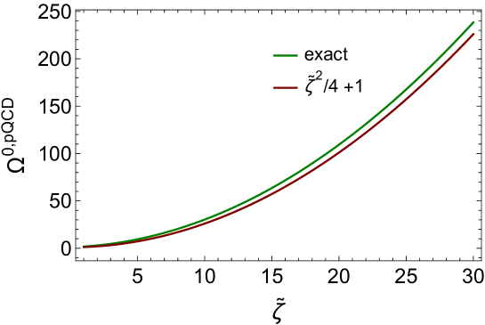
Figure 10: Fig. 10-a: Function versus
. Fig. 10-b: Function versus
In this equation we consider and it is given by Eq. (VI.6). Resulting is equal to555It is worthwhile mentioning that in leading twist approximation for the BFKL kernel since and LETU .
(VI.9)
Finally, we have the implicit solution in the form (see Eq. (III.14) and Eq. (III.15)):
(VI.10)
Using smallness of we can rewrite Eq. (VI.11) as follows:
(VI.11)
where we neglect the contribution in .
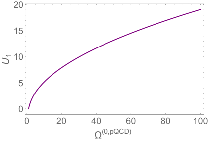
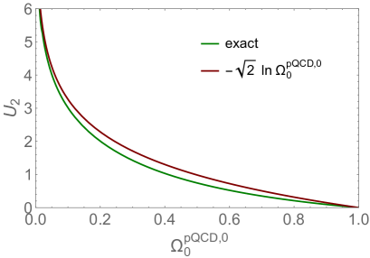
The expression for function it is more convenient to rewrite as follows:
The general solution for the second iteration has the form (see Eq. (V.12)):
(VI.17)
The contribution of we have discussed in section III-C and it can be written as a sum of two contributions:
(VI.18)
We divide the region of integration in two parts: (i) and (ii) . The first region cancels the first term in Eq. (VI.18), while the second gives the main contribution. In the second kinematic region we introduce where . Using this notation we replace by . In the region both
and .
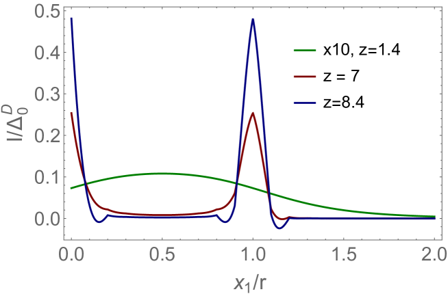
In Fig. 12-a we show the result of integrations.
Figure 12: Fig. 12-a: versus at fixed .
Fig. 12-b: versus .
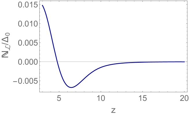
Since is small we can hope that will be small as well (see Fig. 8).
Repeating the estimates in Eq. (V.21) - Eq. (V.22) we obtain
(VI.19)
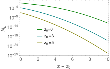
The second term in Eq. (VI.19) decreases with and can be considered as a small correction. However the constant has to be evaluated which are shown in Fig. 12-b.
One can see that that the value of is rather small. Therefore, we have shown that our procedure of solving the nonlinear equation works.
VII Conclusions
In this paper we developed the homotopy approach for solving the non-linear evolution equation for the processes of the diffraction production in DISKOLE . The goal of this approach is to choose the first iteration by the simplified equation which can be solved analytically and includes the main features of the general solution. In our previous paper CLMNEW for such equation the linearised version of the non-linear Balitsky-Kovchegov equationBK was used as the first iteration of the homotopy approachHE1 ; HE2 . In this paper we introduced part of the nonlinear corrections in the first iteration (see Eq. (III.3) for details).
Based on this approach we
found that the first iteration of the homotopy approach gives the main contribution in the both kinematic regions which we consider for the diffractive production: (i) and , where is the value of the rapidity gap; and (ii) and . We also demonstrated that the second iteration of this approach leads to small corrections. Therefore, we can conclude that we found the regular procedure of solving the non-linear equation in which we can take into account the small correction using the regular perturbation approximation.
In the paper we focused mostly on
the kinematic region and . We found that for (see region I in Fig. 1) our solution shows the geometric scaling behaviour, while for (see region II in Fig. 1) this behaviour is strongly violated. We found that the analytical solution of the non-linear equation that has been used as the first interaction, reproduces the intitial and boundary conditions in the both kinematic regions. The second iteration with zero initial and boundary conditions turns out to be small and could be taken into account together with higher iterations using the regular perturbative procedure.
For the kinematic region: and we found that the second iteration is small only f if . It means that for the dipoles with very small sizes we could expect a considerable corrections in the perturbative approximation. We are going to investigate this region in our further publications.
VIII Acknowledgements
We thank our colleagues at Tel Aviv University and UTFSM for encouraging discussions. This research was supported by Fondecyt (Chile) grants No. 1231829 and 1231062.
J.G. express his gratitude to the PhD scholarship USM-DP No. 029/2024 for the financial support.
References
(1)
C. Contreras, E. Levin and R. Meneses,
Phys. Rev. D 107 (2023) no.9, 094030
doi:10.1103/PhysRevD.107.094030
[arXiv:2302.10497 [hep-ph]].
(3)
J.H. He,
Int. J. Nonlinear Mech. 35 (2000) 37.
(4)
I. Balitsky,
Phys. Rev. D60, 014020 (1999);
Y. V. Kovchegov,
Phys. Rev. D60, 034008 (1999).
(5)
Y. V. Kovchegov and E. Levin,
Nucl. Phys. B 577 (2000) 221.
(6)
M. Hentschinski, H. Weigert and A. Schafer,
Phys. Rev. D 73 (2006) 051501,
[hep-ph/0509272].
(7)
Y. Hatta, E. Iancu, C. Marquet, G. Soyez and D. N. Triantafyllopoulos,
Nucl. Phys. A 773 (2006) 95,
[hep-ph/0601150].
(8)
A. Kovner, M. Lublinsky and H. Weigert,
Phys. Rev. D 74 (2006) 114023,
[hep-ph/0608258].
(9)
A. Kormilitzin, E. Levin and A. Prygarin,
Nucl. Phys. A 813 (2008), 1-13
doi:10.1016/j.nuclphysa.2008.09.006
[arXiv:0807.3413 [hep-ph]].
(10)
E. Levin and M. Wusthoff,
Phys. Rev. D 50 (1994), 4306-4327.
(11)
K. J. Golec-Biernat and J. Kwiecinski,
Phys. Lett. B 353 (1995) 329,
[hep-ph/9504230].
(12)
E. Gotsman, E. Levin and U. Maor,
Nucl. Phys. B 493 (1997) 354,
[hep-ph/9606280].
(13)
K. J. Golec-Biernat and M. Wusthoff,
Phys. Rev. D 60 (1999) 114023
[hep-ph/9903358]; Phys. Rev. D 59 (1998) 014017;
[hep-ph/9807513].
(14)
Y. V. Kovchegov and L. D. McLerran,
Phys. Rev. D 60 (1999) 054025
Erratum: [Phys. Rev. D 62 (2000) 019901],
[hep-ph/9903246].
(15)
S. Munier and A. Shoshi,
Phys. Rev. D 69 (2004) 074022,
[hep-ph/0312022].
(16)
C. Marquet and L. Schoeffel,
Phys. Lett. B 639 (2006) 471,
[hep-ph/0606079].
(17)
C. Marquet,
Phys. Rev. D 76 (2007) 094017,
[arXiv:0706.2682 [hep-ph]].
(18)
H. Kowalski, T. Lappi, C. Marquet and R. Venugopalan,
Phys. Rev. C 78 (2008) 045201,
[arXiv:0805.4071 [hep-ph]].
(19)
E. Levin and M. Lublinsky,
Nucl. Phys. A 712 (2002) 95,
[hep-ph/0207374].
(20)
E. Levin and M. Lublinsky,
Eur. Phys. J. C 22 (2002) 64, [hep-ph/0108239].
(21)
Yuri V. Kovchegov and Eugene Levin, “ Quantum Chromodynamics at High Energies", Cambridge Monographs on Particle Physics, Nuclear Physics and Cosmology, Cambridge University Press, 2012 .
(22)
C. Contreras, E. Levin, R. Meneses and I. Potashnikova,
Eur. Phys. J. C 78 (2018) no.6, 475
doi:10.1140/epjc/s10052-018-5957-z
[arXiv:1802.06344 [hep-ph]].
(23)
C. Contreras, E. Levin, R. Meneses and I. Potashnikova,
Eur. Phys. J. C 78 (2018) no.9, 699
doi:10.1140/epjc/s10052-018-6179-0
[arXiv:1806.10468 [hep-ph]].
(24)
A. H. Mueller and S. Munier,
Phys. Rev. D 98 (2018) no.3, 034021
doi:10.1103/PhysRevD.98.034021
[arXiv:1805.02847 [hep-ph]].
(25)
A. H. Mueller and S. Munier,
Phys. Rev. Lett. 121 (2018) no.8, 082001
doi:10.1103/PhysRevLett.121.082001
[arXiv:1805.09417 [hep-ph]].
(26)
A. D. Le, A. H. Mueller and S. Munier,
Phys. Rev. D 104 (2021), 034026
doi:10.1103/PhysRevD.104.034026
[arXiv:2103.10088 [hep-ph]].
(27)
V. A. Abramovsky, V. N. Gribov and O. V. Kancheli,
Yad. Fiz. 18 (1973), 595, (Sov.J. Nucl.Phys. 18 (1974),308);
(28)
L. N. Lipatov,
Sov. Phys. JETP 63, 904 (1986)
[Zh. Eksp. Teor. Fiz. 90, 1536 (1986)].
(29)
L. N. Lipatov,
Phys. Rept. 286 (1997) 131.
(30)
A. H. Mueller and D. N. Triantafyllopoulos,
Nucl. Phys.B640 (2002) 331
[arXiv:hep-ph/0205167]; D. N. Triantafyllopoulos,
Nucl. Phys.B648 (2003) 293
[arXiv:hep-ph/0209121].
(31)
V. S. Fadin, E. A. Kuraev and L. N. Lipatov,
Phys. Lett. B60, 50 (1975);
E. A. Kuraev, L. N. Lipatov and V. S. Fadin,
Sov. Phys. JETP 45, 199 (1977),
[Zh. Eksp. Teor. Fiz.72,377(1977)];
I. I. Balitsky and L. N. Lipatov,
Sov. J. Nucl. Phys. 28, 822 (1978),
[Yad. Fiz.28,1597(1978)].
(32)
E. Levin and K. Tuchin,
Nucl. Phys. B 573, 833 (2000)
[hep-ph/9908317];
Nucl. Phys. A 691, 779 (2001)
[hep-ph/0012167]; 693, 787 (2001)
[hep-ph/0101275].
(33)
J. Bartels and E. Levin,
Nucl. Phys. B 387 (1992), 617-637
doi:10.1016/0550-3213(92)90209-T
(34)
A. M. Stasto, K. J. Golec-Biernat and J. Kwiecinski,
Phys. Rev. Lett. 86 (2001), 596-599
doi:10.1103/PhysRevLett.86.596
[arXiv:hep-ph/0007192 [hep-ph]].
L. McLerran and M. Praszalowicz,
Acta Phys. Polon. B 42 (2011), 99-103
doi:10.5506/APhysPolB.42.99
[arXiv:1011.3403 [hep-ph]];
Phys. Lett. B 741 (2015), 246-251
doi:10.1016/j.physletb.2014.12.046
[arXiv:1407.6687 [hep-ph]].
(35)
K. J. Golec-Biernat and A. M. Stasto,
Nucl. Phys. B 668 (2003), 345-363
[arXiv:hep-ph/0306279 [hep-ph]].
(36)
J. Berger and A. Stasto,
Phys. Rev. D 83 (2011), 034015
[arXiv:1010.0671 [hep-ph]].
(37)
C. Contreras, E. Levin, R. Meneses and M. Sanhueza,
Eur. Phys. J. C 80, no.11, 1029 (2020)
doi:10.1140/epjc/s10052-020-08580-w
[arXiv:2007.06214 [hep-ph]].
(38)
L. V. Gribov, E. M. Levin and M. G. Ryskin,
Phys. Rept. 100, 1 (1983).
(39)
A.D. Polyanin and V.F. Zaitsev,“‘Handbook of nonlinear partial differential equations",CRC press,2004.
(40)
A.D. Polyanin and V.F. Zaitsev,“Handbook of Exact Solutions for Ordinary Differential Equation”,CRC press,1995.
(41)
Andrey D. Polyanin, “Handbook of Linear Differential Equations For Engineers and Scientists", Chapman& Hall/CRC,
2002.
(42)
F.Olver, D. Lozier, R.Boisvert and C. Clark, eds.,“ NIST handbook of Mathematical Functions". U.S. Departament of Commerce, National Institute of Standard and Technology, Cambridge University Press, Wasington, DC, Cambridge, 2010.
(43)
M. Abramowitz and I. Stegun, “Handbook of Mathematical Functions with Formulas, Graphs, and Mathematical Tables”, United States Department of Commerce, National Bureau of Standards,1964.