Universal spectrum of non efimovian three-body resonances at finite scattering length

Abstract

Using exact solutions of the three-body problem, the spectrum of non efimovian three-body resonances for two identical particles interacting with another one is derived in the regime of large but finite scattering length. The universality of the problem is depicted by using a contact model in the generalized effective range approximation, parameterized by two three-body parameters and the scattering length.

The search of universal solutions to the three-body quantum problem begun with the pioneering work of Skorniakov and Ter-Martirosian (STM) Sko57 . Considering the three-nucleon system, they reduced the neutron-deuteron scattering problem to a one-dimensional integral equation. A series of fascinating results on the three bosons problem followed, culminating with the Efimov effect Dan61 ; Min62a ; Min62b ; Efi70 ; Efi71 . Universality means here, that the details of the interactions can be replaced by few parameters in a contact and thus structureless model. This may occur when the dominant interaction among the particles is near the unitary limit of the two-body $s$-wave scattering, such as the neutron-neutron interaction which has led to recent universal predictions in nuclear physics Ham21 . Universality is also an important research focus in ultracold physics, which offers the possibility of tuning the scattering length and to reach the unitary regime with Feshbach resonances Ino98 ; Chi10 . This led to the first observation of the Efimov effect Kra06 . Together with dramatic experimental progress and a detailed analysis of the Efimov effect Nai17 , one can highlight remarkable theoretical results in the three-dimensional case Bed00 ; Pet03 ; Pet04 ; Wer06a ; Kar07a ; Kar07b ; Gog08 .

Aside the Efimov effect which has been thoroughly explored, universal properties of isolated, i.e. non efimovian three-body resonances near the unitary limit have been less studied. Indeed, in most of the cases these resonant states are not square integrable due to the singularity inherent to the contact approach Wer06b ; Gao15 . This ’normalization catastrophe’ has been solved by introducing a modified scalar product Pri23 ; Pri24a . In these last references, using a generalized effective range approximation, it is shown also that in addition to the scattering length, near the threshold of a $N$-body resonance, two parameters (and not one as in the Efimov effect) are in general necessary to describe low energy states. This result follows from a strong analogy with two-body high-partial wave resonances and the presence of a generalized repulsive kinetic barrier in the hyperradius $\rho$. The spectrum at unitarity is given in Refs. Pri23 ; Pri24a , nevertheless, for a finite value of the scattering length ${a}$, the problem was not yet solved. In this situation, the STM equation which is in principle more adapted for finding low energy solutions than solving the Schrödinger equation in the configuration space. However, paradoxically isolated three-body resonances at unitarity are not found in standard numerical analysis of the STM equation. The underlying physics explaining this issue is again the presence of the generalized kinetic barrier which prevents to find any borromean states if a singularity is not somehow imposed at a vanishing hyperradius. Instead, standard computations are only able to recover the Kartavtsev Malyckh (KM) states found in mass-imbalanced systems and which can be viewed as the precursors of the Efimov states. These states appear only in the regime of large but positive scattering length ${a>0}$ and their existence is linked to the presence of the shallow dimer of binding wavenumber ${1/a}$ Kar07a ; Kar07b . As a consequence of the generalized kinetic barrier, the wavefunction of the KM states vanishes at the three-body contact. Like giving a kick in a ball to heard the various resonances of a spherical box, one has to add a source term in the STM equation to excite the desired harmonics which correspond here to singular solutions in the high momentum or equivalently, the small hyperradius limits.

One considers three types of systems: three identical bosons (3B system) of mass $M$, or two non interacting identical fermions [respectively bosons] of mass $M$ interacting with one impurity of mass $m$ (3FI system [respectively 3BI system]) in the center of mass frame. The binary interactions are near the $s$-wave unitary limit. The main results of the present work are as follows: ${i)}$ three-body resonant states are expressed in terms of universal functions which are solutions of the STM equation; ${ii)}$ these solutions are given analytically at the unitary limit and their continuations at finite scattering are obtained by using a Lippmann Schwinger-like equation; ${iii)}$ in the limit of a vanishing detuning, the spectrum is obtained analytically for ${s>1}$, where the index ${s}$ characterizes the singularity of the wavefunction at the three-body contact; otherwise it is deduced from a transcendental equation where only one universal parameter is evaluated numerically for ${s\lesssim 2}$; ${iv)}$ still for ${s>1}$, the width of long-lived quasi-bound states is also dependent on this last universal parameter; ${v)}$ The possibility of endpoints in the KM spectrum is predicted.

In this three-body problem, the particles labelled by $1$ and $2$ are of mass $M$ and the particle labelled by $3$ is of mass $m$. There are three sets of hyperspherical coordinates ${\boldsymbol{\rho}=(\boldsymbol{\rho}^{(ij)}_{1},\boldsymbol{\rho}^{(ij)}_{2})}$, each associated with a given pair $(ij)$. Using the reference mass ${m_{\rm r}=mM/(M+m)}$, the coordinates associated with the pair $(23)$ are ${\boldsymbol{\rho}^{(23)}_{1}=\mathbf{r}_{23}}$ and ${\boldsymbol{\rho}^{(23)}_{2}=\mathbf{r}_{23}\tan\theta-\mathbf{r}_{13}\sec\theta}$ where ${\mathbf{r}_{ij}=\mathbf{r}_{j}-\mathbf{r}_{i}}$ and the angle ${\theta\in[0,\pi/2]}$ is such that ${\sin\theta=m_{\rm r}/m}$. The coordinates ${(\boldsymbol{\rho}^{(12)}_{1},\boldsymbol{\rho}^{(12)}_{2})}$ [respectively ${(\boldsymbol{\rho}^{(31)}_{1},\boldsymbol{\rho}^{(31)}_{2})}$] are deduced from ${(\boldsymbol{\rho}^{(23)}_{1},\boldsymbol{\rho}^{(23)}_{2})}$ by using a $2\times 2$ active rotation matrix of angle $\frac{3\pi}{4}-\frac{\theta}{2}$ [respectively $-\frac{\pi}{2}-\theta$]. Moreover one has the property ${\boldsymbol{\rho}^{(ij)}_{1}=-\boldsymbol{\rho}^{(ji)}_{1}}$ and ${\boldsymbol{\rho}^{(ji)}_{2}=\boldsymbol{\rho}^{(ij)}_{2}}$. For a given value of the $s$-wave scattering length $a$, the interaction between two particles ${(ij)}$ is described by using the Bethe-Peierls condition which imposes a singular behavior of the wavefunction when ${r_{ij}=\rho^{(ij)}_{1}\to 0}$:

$$\langle\boldsymbol{\rho}|\Psi\rangle\operatornamewithlimits{=}_{\rho^{(ij)}_{1}\to 0}\langle\boldsymbol{\rho}^{(ij)}_{2}|A_{ij}\rangle\left({1}/{a}-{1}/{\rho^{(ij)}_{1}}\right)+\dots$$ (1)

In Eq. (1), the state ${|A_{ij}\rangle}$ describes the relative motion of the center of mass of the pair of particles ${(ij)}$ close together with respect to the third particle. It is convenient to introduce a statistical factor $S$ related to the exchange symmetry in the system: for the 3B system ${|A_{12}\rangle=|A_{13}\rangle=|A_{23}\rangle=|A\rangle}$ and ${S=2}$, otherwise ${|A_{12}\rangle=0}$ and for the 2BI system ${|A_{13}\rangle=|A_{23}\rangle=|A\rangle}$ with ${S=1}$, whereas for the 2FI system ${|A_{23}\rangle=-|A_{13}\rangle=|A\rangle}$ with ${S=-1}$. One denotes the energy ${E=-{\hbar^{2}q^{2}}/{(2m_{\rm r})}}$ and $q$ is the binding wavenumber of the system. At unitarity (${|a|=\infty}$) there is a scale invariance and the wavefunction is separable in the hyperradius ${\rho}$ and the hyperangles ${\boldsymbol{\Omega}}$ that parameterize the unit 6-vector ${\boldsymbol{\rho}/\rho}$:

$$\langle\boldsymbol{\rho}|\Psi\rangle=\rho^{-2}F(\rho)\Phi(\boldsymbol{\Omega})\ \text{with}\ F(\rho)\propto K_{s}(q\rho),$$ (2)

where ${\Phi(\boldsymbol{\Omega})}$ is an eigenstate of the Laplacian on the unit hypersphere and satisfies the contact conditions in Eq. (1) with the eigenvalue ${4-s^{2}}$. At finite scattering length, the eigenfunctions are no longer separable and it is convenient to pursue the calculations in the reciprocal space with the wavevectors ${(\boldsymbol{\kappa}^{(ij)}_{1},\boldsymbol{\kappa}^{(ij)}_{2})}$ that are the conjugate of ${(\boldsymbol{\rho}^{(ij)}_{1},\boldsymbol{\rho}^{(ij)}_{2})}$. Isotropy allows one to isolate each component of angular momentum ${\hbar\ell}$ with the ket ${|\mathcal{A}_{\ell}\rangle}$:

$$\langle\mathbf{k}|A\rangle=\langle k|\mathcal{A}_{\ell}\rangle P_{\ell}(\hat{\mathbf{e}}_{\mathbf{k}}\cdot\hat{\mathbf{e}}_{\mathbf{z}}).$$ (3)

The general definition of the hyperradial function is then

$$F(\rho)\propto\rho\langle\rho|\mathcal{A}_{\ell}\rangle.$$ (4)

The Fourier transform that links ${\langle k|\mathcal{A}_{\ell}\rangle}$ to ${\langle\rho|\mathcal{A}_{\ell}\rangle}$ can be expressed with the Hankel transform:

$$\langle k|\mathcal{A}_{\ell}\rangle=\int_{0}^{\infty}\rho^{2}j_{\ell}(k\rho)\langle\rho|A_{\ell}\rangle d\rho.$$ (5)

Considering the contact condition for the pair ${(ij)}$, one obtains after some algebra, the STM equation:

$$\langle k|\mathcal{L}_{\ell,q}^{\infty}|\mathcal{A}_{\ell}\rangle=\langle k|\mathcal{A}_{\ell}\rangle/a,$$ (6)

where $\mathcal{L}_{\ell,q}^{\infty}$ is the following operator

$$\langle k|\mathcal{L}_{\ell,q}^{\Lambda}|\mathcal{A}_{\ell}\rangle=\sqrt{k^{2}+q^{2}}\langle k|\mathcal{A}_{\ell}\rangle-\frac{2S(-1)^{\ell}}{\pi\sin(2\theta)}\\ \times\int_{0}^{\Lambda}\frac{k^{\prime}dk^{\prime}}{k}Q_{\ell}\left(\frac{k^{2}+k^{\prime}\,{}^{2}+q^{2}\cos^{2}\theta}{2kk^{\prime}\sin\theta}\right)\langle k^{\prime}|\mathcal{A}_{\ell}\rangle,$$ (7)

considered at ${\Lambda=\infty}$. At zero energy and in the unitary limit, the STM equation is scale invariant and admits thus power law solutions ${z^{\gamma-2}}$, where ${\gamma}$ is a solution of

$$I_{\ell,\gamma}={\sin 2\theta}/{(2S)}$$ (8)

and the function ${I_{\ell,\gamma}}$ is defined by

$$I_{\ell,\gamma}=(-1)^{\ell}\int_{0}^{\infty}\frac{dv}{\pi}Q_{\ell}\left(\frac{v^{2}+1}{2v\sin\theta}\right)v^{\gamma-1}.$$ (9)

This last quantity satisfies the recurrence relation:

$$I_{\ell+1,\gamma}=-\frac{(2\ell+1)\left(I_{\ell,\gamma-1}+I_{\ell,\gamma+1}\right)}{2(\ell+1)\sin\theta}-\frac{\ell I_{\ell-1,\gamma}}{\ell+1}$$ (10)

valid for ${\ell\geq 0}$ and set by the initial condition

$$I_{0,\gamma}={\sin(\gamma\theta)}/[{\gamma\cos(\gamma\pi/2)}].$$ (11)

Using the fact that ${I_{\ell,\gamma}=I_{\ell,-\gamma}}$, the solutions of Eq. (70) are given by pairs ${\pm\gamma}$ for a given ${\ell}$. They coincide with the one obtained in the configuration space Wer06a . In the region where the wavefunction is separable as Eq. (2), the function ${F(\rho)}$ satisfies a 2D Schrödinger equation with a generalized kinetic barrier ${\hbar^{2}\gamma^{2}/(2m_{\rm r}\rho^{2})}$ Pri23 . If one considers the reference (i.e. physical) model where the interactions are of finite range and which is mapped to the contact model, this kinetic barrier is truncated at short hyperradius for ${\rho<R_{0}}$ where the particles feel the actual interactions. The length ${R_{0}}$ defines the high energy scale ${E_{0}=\hbar^{2}/(2m_{\rm r}R_{0}^{2})}$ such that when the interparticle distances are larger than ${R_{0}}$, the actual wavefunction can be approximated by the contact wavefunction. In the study of non efimovian three-body resonances for a given ${S}$, one excludes the sectors of ${\ell}$ where there is a solution ${\gamma^{2}<0}$ corresponding to an attractive inverse square hyperradial potential which gives the Efimov effect. At finite energy and/or finite scattering length, the contact states are still characterized by the singularity of the hyperradial function ${F(\rho)\propto\rho^{-|\gamma|}}$ at the three-body contact where ${\rho\to 0}$. One then considers for fixed values ${S}$ and ${\ell}$, the lowest index ${s=|\gamma|}$ corresponding to the lowest kinetic barrier. This gives the asymptotic behavior ${\langle k|\mathcal{A}_{\ell}\rangle=O(k^{-2+s})}$ when ${k\to\infty}$. It is convenient to introduce the reduced wavenumber ${z={k}/{q}}$ and the dimensionless operator ${\mathcal{L}^{\Lambda}}$ obtained by the substitution ${q\to 1}$ and ${(k,k^{\prime})\to(z,z^{\prime})}$ in Eq. (7). The solutions of Eq. (6) can be expressed in terms of universal functions denoted by ${\langle z|\phi_{\ell,s,\tau}\rangle\equiv\langle k|\mathcal{A}_{\ell}\rangle}$ which satisfy the equation

$$\langle z|\mathcal{L}^{\infty}-\tau|\phi_{\ell,s,\tau}\rangle=0\quad\text{with}\quad\tau={1}/{qa}<1.$$ (12)

The universal functions can be represented in a series expansion of the variable ${1/z}$:

$$\langle z|\phi_{\ell,s,\tau}\rangle=z^{s-2}\left(1+\sum_{n=1}^{\infty}c_{\ell,-s,\tau}^{(n)}z^{-n}\right)\\ -r_{\ell,s,\tau}z^{-s-2}\left(1+\sum_{n=1}^{\infty}c_{\ell,s,\tau}^{(n)}z^{-n}\right)$$ (13)

The two terms in the right-hand-side of Eq. (13) are two independent solutions of Eq. (12) and the coefficient ${r_{\ell,s,\tau}}$ is such that ${\langle z|\phi_{\ell,s,\tau}\rangle=O(z^{\ell})}$ when ${z\to 0}$ (a behavior deduced from Eq. (5)) . The coefficients ${c_{\ell,\gamma,\tau}^{(n)}}$ for $\gamma=\pm s$ can be deduced by recurrence after injection of Eqs. (13) in Eq. (12). At unitarity where ${\tau=0}$, the universal functions are obtained directly from Eqs. (2,4,5):

$$\langle z|\phi_{0,s,0}\rangle=2^{1-s}\frac{\sinh\left[s\operatorname{arcsinh}(z)\right]}{z\sqrt{1+z^{2}}}$$ (14)

$$\langle z|\phi_{1,s,0}\rangle=\frac{2^{1-s}}{(s-1)}\frac{d}{dz}\left(\frac{\sinh\left[s\operatorname{arcsinh}(z)\right]}{z}\right)$$ (15)

and for higher values of ${\ell}$, one has the recurrence

$$\langle z|\phi_{\ell+1,s,0}\rangle=\frac{(s+\ell)\langle z|\phi_{\ell-1,s,0}\rangle}{s-\ell-1}+\frac{(2\ell+1)\langle z|\phi_{\ell,s+1,0}\rangle}{z(\ell+1-s)}\\ +\frac{(2\ell+1)(s+\ell)\langle z|\phi_{\ell,s-1,0}\rangle}{4zs(1-s)}.$$ (16)

The trick to find the universal functions at finite scattering length, is to introduce a remainder which plays the role of a source term in Eq. (12) and is a bit like the ’kick in the ball’. To do this, one performs the split

$$\mathcal{L}^{\infty}=\mathcal{L}^{\Lambda}+\delta\mathcal{L}^{\Lambda}.$$ (17)

In the limit ${z\gg 1}$, one has ${\langle z|\phi_{\ell,s,\tau}\rangle\simeq\langle z|\phi_{s,\ell,0}\rangle}$ and thus for a sufficiently large value of the cut-off ${\Lambda}$ and ${z\ll\Lambda}$:

$$\langle z|\delta\mathcal{L}^{\Lambda}|\phi_{\ell,s,\tau}\rangle\simeq\langle z|\delta\mathcal{L}^{\Lambda}|\phi_{\ell,s,0}\rangle.$$ (18)

Using first, the fact that ${|\phi_{\ell,s,0}\rangle}$ is an exact solution of Eq. (12) and second, the approximation in Eq. (18) which is exact in the limit ${\Lambda\gg 1}$, Eq. (12) can be written:

$$(\mathcal{L}^{\Lambda}-\tau)|\phi_{\ell,s,\tau}\rangle\underset{\Lambda\gg 1}{=}\mathcal{L}^{\Lambda}|\phi_{\ell,s,0}\rangle$$ (19)

This last equation can be solved in the non efimovian regime in a form analogous to the Lippmann-Schwinger equation Empirically ; limit :

$$|\phi_{\ell,s,\tau}\rangle=|\phi_{\ell,s,0}\rangle+\tau\lim_{\Lambda\to\infty}(\mathcal{L}^{\Lambda}-\tau)^{-1}|\phi_{\ell,s,0}\rangle.$$ (20)

As shown in Ref. Pri24a , the three-body contact condition can be replaced in the generalized effective range approximation by an energy dependent log-derivative condition at the finite hyperradius $R_{0}$ Danilov :

$$\frac{\rho\partial_{\rho}F(\rho)}{F(\rho)}\biggr{|}_{\rho=R_{0}}=-\upsilon_{0}+\upsilon_{0}^{\prime}q^{2}R_{0}^{2},$$ (21)

where ${\upsilon_{0}}$ and ${\upsilon_{0}^{\prime}}$ are the two three-body parameters set by the actual interactions of the physical system considered. The function $F(\rho)$ is then expanded in terms of the variable $\underline{z}=q\rho$ as:

$$F(\rho)=\underline{z}^{-s}\left(1+\sum_{n=1}^{\infty}\underline{c}_{\ell,-s,\tau}^{(n)}\underline{z}^{n}\right)-\frac{\Gamma(1+\ell-s)}{\Gamma(1+\ell+s)}\\ \times{r}_{\ell,s,\tau}\underline{z}^{s}\left(1+\sum_{n=1}^{\infty}\underline{c}_{\ell,s,\tau}^{(n)}\underline{z}^{n}\right).$$ (22)

The coefficients ${\underline{c}_{\ell,\gamma,\tau}^{(n)}}$ in Eq. (22) are deduced from the expansion in Eq. (13) by using the inverse transform of Eq. (5). In the generalized effective range approximation, Eq. (22) is truncated at the second order ${(n=2)}$ with:

$$\underline{c}_{\ell,-s,\tau}^{(1)}=\frac{\tau I_{\ell,s}\Gamma\left(1+\frac{\ell-s}{2}\right)\Gamma\left(\frac{\ell+s}{2}\right)}{2\left(I_{\ell,s}-I_{\ell,1-s}\right)\Gamma\left(\frac{1}{2}+\frac{\ell+s}{2}\right)\Gamma\left(\frac{3}{2}+\frac{\ell-s}{2}\right)}$$ (23)

$$\underline{c}_{\ell,-s,\tau}^{(2)}=1/(4-4s)+\left(\tau I_{\ell,s}\right)^{2}/[(\ell+2-s)(\ell-1+s)]$$

$$\qquad\qquad\qquad\qquad/[(I_{\ell,s}-I_{\ell,1-s})(I_{\ell,s}-I_{\ell,2-s})].$$ (24)

Injection of Eq. (22) in Eq. (21) gives for ${s<1+\eta}$:

$$\frac{1}{\xi_{s}(R_{0}/a)}+\frac{E}{E_{0}}\frac{\alpha_{s}}{R_{0}^{2}}=\frac{r_{\ell,s,\tau}(-E/E_{0})^{s}}{r_{\ell,s,0}\sin(\pi s)R_{0}^{2s}},$$ (25)

where the positive parameter ${\eta}$ tends to zero in the limit of a vanishing detuning $s-\upsilon_{0}$ and for a small but finite detuning, one uses typically ${\eta\sim.3}$. For larger values of ${s}$, at the order of the generalized effective range approximation, the ratio term in the right-hand-side of Eq. (25) is neglected in the calculation of the real part of the energy other_words . At unitarity, the resonance threshold ${E=0}$ is at $\upsilon_{0}=s$. In Eq. (25), $\alpha_{s}$ is the range parameter:

$$\alpha_{s}=\frac{s4^{s}(s-\upsilon_{0})\Gamma(s)^{2}}{\pi(s+\upsilon_{0})R_{0}^{2s-2}}\biggl{(}\frac{\upsilon_{0}^{\prime}+\frac{2+\upsilon_{0}-s}{4(s-1)}}{s-\upsilon_{0}}-{s\leftrightarrow-s}\biggr{)}$$ (26)

and ${\xi_{s}(R_{0}/a)}$ is the generalized scattering length:

$$\xi_{s}\left(\frac{R_{0}}{a}\right)=\frac{\pi R_{0}^{2s}}{s4^{s}\Gamma(s)^{2}}\times\Biggl{[}\frac{\bigl{(}\frac{R_{0}^{2}}{a^{2}}\left(\upsilon_{0}+s+2\right)\frac{d\underline{c}_{\ell,s,\tau}^{(2)}}{d(\tau^{2})}\quad}{}\\ \frac{\quad+\frac{R_{0}}{a}\left(\upsilon_{0}+s+1\right)\frac{\underline{c}_{\ell,s,\tau}^{(1)}}{\tau}+\upsilon_{0}+s\bigr{)}}{\left(s\leftrightarrow-s\right)}\Biggr{]}.$$ (27)

The expressions of ${\xi_{s}(0)}$ and ${\alpha_{s}}$ were already obtained in Ref. Pri24a . For $s<1+\eta$, the ratio ${r_{\ell,s,\tau}}$ can be evaluated with a good precision from the numerical solutions of Eq. (20). Solutions of Eq. (25) are detailed in the following lines. The pure KM states exist only when ${a>0}$ and are regular solutions of Eq. (12), i.e. ${|r_{\ell,s,\tau}|=\infty}$ corresponding to specific values of ${\tau=\tau_{\infty,n}}$ of the order of unity, where ${n=1,2\dots}$ labels the KM states. Their number depends on the statistics, the angular momentum and the mass ratio. These states are modified by the log-derivative condition as follows. From Eq. (25) the KM spectrum is obtained in the limit ${E\to 0}$ from the solutions of

$$r_{\ell,s,\tau}\simeq a^{2s}r_{\ell,s,0}\sin(\pi s)\tau^{2s}/\xi_{s}(R_{0}/a).$$ (28)

At each KM state ${(n)}$ is associated a branch of the ratio ${r_{\ell,s,\tau}}$ considered as function of $\tau$, with a vertical asymptote located at ${\tau=\tau_{\infty,n}}$. For a given branch, in the limit of large and positive scattering length, one recovers the pure KM state from Eq. (28) with ${q\simeq 1/(a\tau_{\infty,n})}$. For decreasing values of ${a}$, the KM state asymptotically follows the law ${q\simeq 1/(a\tau_{0,n})}$ where ${r_{\ell,s,\tau_{0,n}}=0}$. Importantly, the spectrum of the shallowest KM state has an endpoint on the two-body spectrum if Eq. (28) has a solution at ${\tau=1}$. Concerning the three-body resonances, a shallow bound state occurs for a small and negative detuning ${s-\upsilon_{0}}$, i.e. when ${\xi_{s}(0)\gg R_{0}^{2s}}$. One first considers the regime of small index ${s<1+\eta}$, i.e. not far from the Efimov threshold, as for instance in the 2FI system when ${\ell=1}$ and for a mass ratio ${8.6\dots\lesssim x<13.6\dots}$. In the limit ${s\ll 1}$ and using the behavior ${r_{\ell,s,\tau}=O\left((-\tau)^{2s}\right)}$ when ${\tau\to-\infty}$, one finds the endpoint ${a^{(-)}=a^{(-)}_{\rm as}}$:

$${a^{(-)}_{\rm as}}=\lim_{\tau\to-\infty}({r_{\ell,s,\tau}}/{r_{\ell,s,0}})^{{1}/{2s}}/(q_{\rm u}\tau).$$ (29)

where ${q_{u}}$, is the wavenumber at unitarity when the range parameter is negligible in Eq. (25):

$$q_{\rm u}=\frac{2}{R_{0}}\left[\frac{s\sin(\pi s)\Gamma(s)^{2}(\upsilon_{0}-s)}{\pi(\upsilon_{0}+s)}\right]^{{1}/{2s}}.$$ (30)

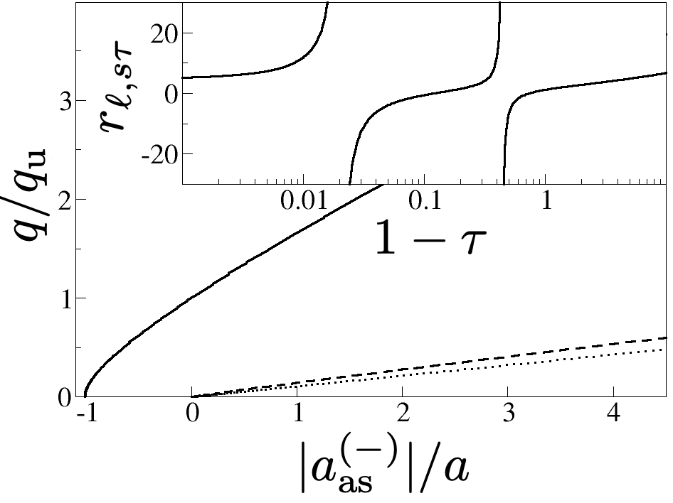
Figure 1: Binding wavenumber as a function of the inverse scattering length for ${\ell=1}$, ${S=-1}$, ${s=.2}$, ${s-\upsilon_{0}=-10^{-2}}$ and ${\upsilon_{0}^{\prime}=.5}$. The asymptotic value of the endpoint $a^{(-)}_{\rm as}$ is given in Eq. (29). The wavenumber $q_{\rm u}$ is given in Eq. (30). Solid line: three-body resonant state; dashed line: deepest KM state; dotted line: shallow dimer spectrum. Inset: plot of the ratio ${r_{\ell,s,\tau}}$.

An example where ${s<1+\eta}$ is illustrated in Fig. (1) by considering the 3FI system for ${\ell=1}$ and ${s=.2}$. In this example, ${a^{(-)}_{\rm as}}=-9.9\times 10^{4}R_{0}$ and Eqs. (29,30) are very good approximations. The ratio plotted in the inset of the figure has two branches with vertical asymptotes and consequently there are two KM states is this example. The spectrum of the deepest KM state is plotted with the dashed line. In this example, the excited KM state associated with the first branch of the ratio is almost degenerate with the dimer spectrum near the unitary limit and has an endpoint at a very large scattering length with ${R_{0}/a\simeq 2.9\times 10^{-6}}$. One considers now the regime where ${s>1+\eta}$. Away from an eventual crossing with a KM state, the ratio term can be neglected so that crossing :

$$E\simeq-\hbar^{2}/\left[2m_{\rm r}\alpha_{s}\xi_{s}(R_{0}/a)\right].$$ (31)

In this regime, the endpoint at the three-body continuum is obtained from the equation ${\xi_{s}(R_{0}/a^{(-)})=\infty}$:

$${a^{(-)}}\simeq{R_{0}}{\underline{c}^{(1)}_{\ell,-s,\tau}}/{[\tau(s-\upsilon_{0})]}.$$ (32)

For a small and positive value of the detuning ${s-\upsilon_{0}}$, the generalized scattering length is large and negative in the vicinity of unitarity, one gets a long-lived quasi-bound state when ${s\geq 1}$ and even for smaller values of ${s}$ if ${\upsilon_{0}^{\prime}}$ is sufficiently large. This corresponds to a complex energy solution of Eq. (25): ${E=E_{\rm r}-{i\Gamma}/{2}}$ where ${E_{\rm r}}$ is given by Eq. (31). The leading contribution to the expression of the width ${\Gamma}$ is obtained from the ratio term:

$$\frac{\Gamma}{E_{\rm r}}\simeq\frac{2\Re(r_{\ell,s,\tau_{\rm r}})}{\alpha_{s}r_{\ell,s,0}}\left(\frac{E_{\rm r}}{E_{0}R_{0}^{2}}\right)^{s-1},\ \tau_{\rm r}=\frac{i\hbar}{a\sqrt{2m_{\rm r}E}}.$$ (33)

The evaluation of the ratio ${r_{\ell,s,\tau_{\rm r}}}$ where ${\tau_{\rm r}\neq 0}$ is complex and ${s}$ is possibly large, is an open issue.

To conclude, the observation of non efimovian three-body resonances in ultracold atoms has not been yet achieved and is challenging. The 2FI atomic system composed of two ¹⁷¹Yb and one caesium is an interesting candidate for this purpose Pri23 . As predicted generically in Ref. Nai22 , a three-body resonance is expected to occur in this system ${(\ell=1,s\simeq 1.73)}$ from the combination of a Yb-Yb $p$-wave optical Feshbach resonance and a Yb-Cs $s$-wave magnetic Feshbach resonance Goy10 ; Yama13 ; Yang19 . Using another alkali for the impurity as sodium or potassium offers the opportunity to explore the spectrum for other mass ratios. In this example, the underlying physics explaining the three-body resonance emerges from the presence of a potential well between the two identical fermions that overcomes the two-body kinetic barrier at short distance and which is at the birth of the two-body $p$-wave resonance. In the three-body system the particles experience also this attraction, that may overcome again the generalized kinetic barrier at short hyperradius, leading to a three-body resonance in the system. On this basis, one expects a similar effect for two-body resonances in higher partial waves. Another scenario for a three-body resonance is to consider a Feshbach coupling between the three particles and a three-body molecular state in a closed channel instead of the tunneling effect between the three particles outside the generalized kinetic barrier and the state mainly localized in the well.

Supplemental material

This supplemental material gathers the technical details and steps used in the derivation of the results in the main text. The Jacobi variables used in this work are a particular choice of their general definition in Sec. .1 with a reference mass equals to the reduced mass of the two identical particles. Even if the STM equation is well known, for completeness a derivation is proposed in Sec. .2. The way to derive the expressions of the coefficients ${c_{\ell,s,\tau}^{(1)}}$ and ${c_{\ell,s,\tau}^{(2)}}$ in the expansion of the universal functions and their analog ${\underline{c}_{\ell,s,\tau}^{(1)}}$ and ${\underline{c}_{\ell,s,\tau}^{(2)}}$ in the expansion of the hyperradial functions is detailed in Sec. .3. The recurrence relation satisfied by the universal functions in the unitary limit is detailed in Sec. .4. Finally, Sec. .5 gives the details for the numerical evaluation of the universal functions.

.1 Jacobi coordinates

For a given reference mass $m_{\rm r}$, the three systems of hyperspherical coordinates associated with each possible pair of particles $(ij)$ are defined as follows

$$\boldsymbol{\rho}^{(ij)}_{1}=\sqrt{\frac{\mu_{ij}}{m_{\rm r}}}(\mathbf{r}_{j}-\mathbf{r}_{i})\ ;\ \boldsymbol{\rho}^{(ij)}_{2}=\sqrt{\frac{\mu_{ij,l}}{m_{\rm r}}}\left(\mathbf{r}_{l}-\frac{m_{i}\mathbf{r}_{i}+m_{j}\mathbf{r}_{j}}{m_{i}+m_{j}}\right)\ ;\ \boldsymbol{\rho}_{3}=\frac{m_{1}\mathbf{r}_{1}+m_{2}\mathbf{r}_{2}+m_{3}\mathbf{r}_{3}}{\sqrt{m_{\rm r}(m_{1}+m_{2}+m_{3})}},$$ (34)

where the three integers ${(i,j,l)}$ represent cyclic permutations of the triplet ${(123)}$ and the reduced masses are given by

$$\mu_{ij}=\frac{m_{i}m_{j}}{m_{i}+m_{j}}\quad;\quad\mu_{ij,l}=\frac{m_{l}(m_{i}+m_{j})}{m_{1}+m_{2}+m_{3}}.$$ (35)

The three wave vectors conjugate with the hyperspherical coordinates are

$$\boldsymbol{\kappa}^{(ij)}_{1}=\sqrt{\frac{m_{\rm r}}{\mu_{ij}}}\frac{m_{i}\mathbf{k}_{j}-m_{j}\mathbf{k}_{i}}{m_{i}+m_{j}}\ ;\ \boldsymbol{\kappa}^{(ij)}_{2}=\sqrt{\frac{m_{\rm r}}{\mu_{ij,l}}}\frac{(m_{i}+m_{j})\mathbf{k}_{l}-m_{l}(\mathbf{k}_{i}+\mathbf{k}_{j})}{m_{1}+m_{2}+m_{3}}\ ;\ \boldsymbol{\kappa}_{3}=\sqrt{\frac{m_{\rm r}}{m_{1}+m_{2}+m_{3}}}\left(\mathbf{k}_{1}+\mathbf{k}_{2}+\mathbf{k}_{3}\right).$$ (36)

In this work, one considers mass imbalanced systems where ${m_{1}=m_{2}=M}$ and ${m_{3}=m}$ with the mass ratio ${x=M/m}$ and all the equations are derived with the choice of reference mass $m_{\rm r}=\mu_{13}=\mu_{23}$ which simplifies all the expressions. In the center of mass frame, only the two vectors $(\boldsymbol{\rho}_{1}^{(ij)},\boldsymbol{\rho}_{2}^{(ij)})$ are relevant. They are given by

$$\left\{\begin{array}[]{l}\boldsymbol{\rho}^{(23)}_{1}=\mathbf{r}_{23}\\ \boldsymbol{\rho}^{(23)}_{2}=\frac{1+x}{\sqrt{1+2x}}\left(\mathbf{r}_{1}-\frac{x\mathbf{r}_{2}+\mathbf{r}_{3}}{1+x}\right)\end{array}\right.\ ;\ \left\{\begin{array}[]{l}\boldsymbol{\rho}^{(13)}_{1}=\mathbf{r}_{13}\\ \boldsymbol{\rho}^{(13)}_{2}=\frac{1+x}{\sqrt{1+2x}}\left(\mathbf{r}_{2}-\frac{x\mathbf{r}_{1}+\mathbf{r}_{3}}{1+x}\right)\end{array}\right.\ ;\ \left\{\begin{array}[]{l}\boldsymbol{\rho}^{(12)}_{1}=\sqrt{\frac{1+x}{2}}\mathbf{r}_{12}\\ \boldsymbol{\rho}^{(12)}_{2}=\sqrt{\frac{2(1+x)}{1+2x}}\left(\mathbf{r}_{3}-\frac{\mathbf{r}_{1}+\mathbf{r}_{2}}{2}\right)\end{array}\right.$$ (37)

and the wavevectors of the three sets are given by

$$\left\{\begin{array}[]{l}\boldsymbol{\kappa}^{(23)}_{1}=\frac{x\mathbf{k}_{3}-\mathbf{k}_{2}}{1+x}\\ \boldsymbol{\kappa}^{(23)}_{2}=\frac{\sqrt{1+2x}}{1+x}\mathbf{k}_{1}\end{array}\right.\ ;\ \left\{\begin{array}[]{l}\boldsymbol{\kappa}^{(13)}_{1}=\frac{x\mathbf{k}_{3}-\mathbf{k}_{1}}{1+x}\\ \boldsymbol{\kappa}^{(13)}_{2}=\frac{\sqrt{1+2x}}{1+x}\mathbf{k}_{2}\end{array}\right.\ ;\ \left\{\begin{array}[]{l}\boldsymbol{\kappa}^{(12)}_{1}=\sqrt{\frac{2}{1+x}}(\mathbf{k}_{2}-\mathbf{k}_{1})\\ \boldsymbol{\kappa}^{(12)}_{2}=\sqrt{\frac{1+2x}{2(1+x)}}\mathbf{k}_{3}.\end{array}\right.$$ (38)

The hyperradius $\rho=\sqrt{(\rho^{(ij)}_{1})^{2}+(\rho^{(ij)}_{2})^{2}}$ and the hyperwavenumber $\kappa=\sqrt{(\kappa^{(ij)}_{1})^{2}+(\kappa^{(ij)}_{2})^{2}}$ are invariant in the choice of the pair $(ij)$. One has

$$\rho=\sqrt{\frac{1+x}{1+2x}}\times\sqrt{r_{13}^{2}+r_{23}^{2}+xr_{12}^{2}}=\sum_{i=1}^{3}\frac{m_{i}}{m_{\rm r}}(\mathbf{r}_{i}-\mathbf{C})^{2},$$ (39)

where $\mathbf{C}$ is the center of mass:

$$\mathbf{C}=\frac{x(\mathbf{r}_{1}+\mathbf{r}_{2})+\mathbf{r}_{3}}{1+2x}.$$ (40)

For convenience one also introduces the angle ${\theta\in[0,\pi/2]}$ which satisfies

$$\sin\theta=\frac{x}{1+x}\quad,\quad\cos\theta=\frac{\sqrt{1+2x}}{1+x}.$$ (41)

One can write the Jacobi coordinates as:

$$\boldsymbol{\rho}^{(23)}_{2}=\mathbf{r}_{23}\tan\theta+\mathbf{r}_{31}\sec\theta\quad;\quad\boldsymbol{\rho}^{(13)}_{2}=\mathbf{r}_{13}\tan\theta+\mathbf{r}_{32}\sec\theta$$ (42)

and

$$\boldsymbol{\rho}^{(12)}_{1}=\mathbf{r}_{12}\cos\left(\frac{\pi}{4}-\frac{\theta}{2}\right)\sec\theta\quad\text{or}\quad\boldsymbol{\rho}^{(12)}_{2}=\left(\mathbf{r}_{13}+\mathbf{r}_{23}\right)\sin\left(\frac{\pi}{4}-\frac{\theta}{2}\right)\sec\theta,$$ (43)

where one has used the two identities:

$$\cos\left(\frac{\pi}{4}-\frac{\theta}{2}\right)=\sqrt{\frac{1+\sin\theta}{2}}\quad;\quad\sin\left(\frac{\pi}{4}-\frac{\theta}{2}\right)=\sqrt{\frac{1-\sin\theta}{2}}.$$ (44)

Introducing the $2\times 2$ active rotation matrix

$$\mathcal{R}(\alpha)=\left[\begin{array}[]{cc}\cos\alpha&-\sin\alpha\\ \sin\alpha&\cos\alpha\end{array}\right],$$ (45)

the different set of coordinates are related the ones to the others by a rotation:

$$\left[\begin{array}[]{c}\boldsymbol{\rho}^{(12)}_{1}\\ \boldsymbol{\rho}^{(12)}_{2}\end{array}\right]=\mathcal{R}\left(\frac{3\pi}{4}-\frac{\theta}{2}\right)\left[\begin{array}[]{c}\boldsymbol{\rho}^{(23)}_{1}\\ \boldsymbol{\rho}^{(23)}_{2}\end{array}\right]\ ;\ \left[\begin{array}[]{c}\boldsymbol{\rho}^{(13)}_{1}\\ \boldsymbol{\rho}^{(13)}_{2}\end{array}\right]=\mathcal{R}\left(\frac{\pi}{2}+\theta\right)\left[\begin{array}[]{c}\boldsymbol{\rho}^{(32)}_{1}\\ \boldsymbol{\rho}^{(32)}_{2}\end{array}\right]\ ;\ \left[\begin{array}[]{c}\boldsymbol{\rho}^{(13)}_{1}\\ \boldsymbol{\rho}^{(13)}_{2}\end{array}\right]=\mathcal{R}\left(\frac{\theta}{2}-\frac{3\pi}{4}\right)\left[\begin{array}[]{c}\boldsymbol{\rho}^{(21)}_{1}\\ \boldsymbol{\rho}^{(21)}_{2}\end{array}\right].$$ (46)

One has also the property

$$\left[\begin{array}[]{c}\boldsymbol{\rho}^{(ij)}_{1}\\ \boldsymbol{\rho}^{(ij)}_{2}\end{array}\right]=\mathcal{R}\left(\alpha\right)\left[\begin{array}[]{c}\boldsymbol{\rho}^{(kl)}_{1}\\ \boldsymbol{\rho}^{(kl)}_{2}\end{array}\right]\quad\Longleftrightarrow\quad\left[\begin{array}[]{c}\boldsymbol{\rho}^{(ji)}_{1}\\ \boldsymbol{\rho}^{(ji)}_{2}\end{array}\right]=\mathcal{R}\left(-\alpha\right)\left[\begin{array}[]{c}\boldsymbol{\rho}^{(lk)}_{1}\\ \boldsymbol{\rho}^{(lk)}_{2}\end{array}\right].$$ (47)

.2 STM equation

One starts by writing down the stationary Schrödinger equation in the configuration space at energy ${E=-\frac{\hbar^{2}q^{2}}{2m_{\rm r}}}$:

$$\left(q^{2}-\Delta_{\boldsymbol{\rho}_{1}}-\Delta_{\boldsymbol{\rho}_{2}}\right)\langle\boldsymbol{\rho}|\Psi\rangle=-4\pi\sum_{i<j}\delta(\boldsymbol{\rho}^{(ij)}_{1})\langle\boldsymbol{\rho}^{(ij)}_{2}|A_{ij}\rangle.$$ (48)

The delta distributions in the right-hand-side of Eq. (48) are obtained from the action of a three dimensional Laplacian on the inverse radius singularity inherent of the Bethe-Peierls contact condition of two interacting particles. One then uses the vectors ${(\boldsymbol{\kappa}^{(ij)}_{1},\boldsymbol{\kappa}^{(ij)}_{2})}$ in the reciprocal space, which are the conjugate of ${(\boldsymbol{\rho}^{(ij)}_{1},\boldsymbol{\rho}^{(ij)}_{2})}$ and performs a Fourier transform of Eq. (48). For convenience, one use the short-hand notations ${(\mathbf{p},\mathbf{k})=(\boldsymbol{\kappa}^{(23)}_{1},\boldsymbol{\kappa}^{(23)}_{2})}$, ${\mathbf{k}^{\prime}=\boldsymbol{\kappa}^{(13)}_{2}}$ and ${\mathbf{k}^{\prime\prime}=\boldsymbol{\kappa}^{(12)}_{2}}$. In the center of mass frame:

$$\mathbf{p}=-\mathbf{k}_{1}\sin\theta-\mathbf{k}_{2}\ ;\ \mathbf{k}=\mathbf{k}_{1}\cos\theta.$$ (49)

The Fourier transform of Eq. (48) gives for negative energy states :

$$\langle\mathbf{p},\mathbf{k}|\Psi\rangle=-\frac{4\pi}{q^{2}+k^{2}+p^{2}}\left(\langle\mathbf{k}|A_{23}\rangle+\langle\mathbf{k}^{\prime}|A_{23}\rangle+\langle\mathbf{k}^{\prime\prime}|A_{12}\rangle\right).$$ (50)

The singularity ${1/\rho_{1}^{(23)}}$ at the two-body contact $(2=3)$ is of the same type as the singularity of the two-body Green’s function of the Helmholtz equation at the imaginary wavenumber ${i\lambda}$:

$$\int\frac{d^{3}p}{(2\pi)^{3}}\frac{e^{i\mathbf{p}\cdot\boldsymbol{\rho}^{(23)}_{1}}}{p^{2}+\lambda^{2}}=\frac{\exp(-\lambda\rho^{(23)}_{1})}{4\pi\rho^{(23)}_{1}}.$$ (51)

The contact condition for the pair ${(23)}$, i.e. ${\langle\boldsymbol{\rho}|\Psi\rangle=\langle\boldsymbol{\rho}^{(23)}_{2}|A_{23}\rangle\left({1}/{a}-{1}/{\rho^{(23)}_{1}}\right)+\dots}$ when ${\rho^{(23)}_{1}\to 0}$, can be then implemented by subtracting the inverse radius singularity in the inverse Fourier transform of Eq. (50) performed with respect to the variable ${\mathbf{p}}$ and by taking the limit ${\rho^{(23)}_{1}\to 0}$ :

$$\int\frac{d^{3}p}{(2\pi)^{3}}\left[\langle\mathbf{p},\mathbf{k}|\Psi\rangle+\frac{4\pi\langle\mathbf{k}|A_{23}\rangle}{p^{2}+\lambda^{2}}\right]=\langle\mathbf{k}|A_{23}\rangle\left(\frac{1}{a}-\lambda\right),$$ (52)

where the parameter ${\lambda>0}$ is arbitrary. One then injects Eq. (50) in the integral term of the left-hand-side of Eq. (52) and make the choice ${\lambda=\sqrt{k^{2}+q^{2}}}$ simplifies the resulting equation:

$$\int\frac{d^{3}p}{(2\pi)^{3}}\frac{\langle\mathbf{k}^{\prime}|A_{13}\rangle+\langle\mathbf{k}^{\prime\prime}|A_{12}\rangle}{p^{2}+k^{2}+q^{2}}\\ =\frac{\langle\mathbf{k}|A_{23}\rangle}{4\pi}\left(\sqrt{k^{2}+q^{2}}-\frac{1}{a}\right).$$ (53)

Depending on the system considered and using the exchange symmetry, the states ${|A_{ij}\rangle}$ are expressed in terms of the single state ${|A\rangle}$ as given in Tab. (1).

System	Symmetry	$S$	${{M}/{m}}$
3B	$|A_{12}\rangle=|A_{13}\rangle=|A_{23}\rangle=|A\rangle$	2	x=1
2BI	$|A_{12}\rangle=0$ $|A_{23}\rangle=|A_{13}\rangle=|A\rangle$	1	x
2FI	$|A_{12}\rangle=0$ $|A_{23}\rangle=-|A_{13}\rangle=|A\rangle$	-1	x

Table 1: Three types of systems are considered in the STM equation: three bosons (3B), two bosons and one impurity (2BI), two fermions and one impurity (2FI). The masses of the three particles are given by ${m_{1}=m_{2}=M}$ and ${m_{3}=m}$.

Equation (53) can be then simplified as

$$S\int\frac{d^{3}p}{(2\pi)^{3}}\frac{\langle\mathbf{k}^{\prime}|A\rangle}{p^{2}+k^{2}+q^{2}}=\frac{\langle\mathbf{k}|A\rangle}{4\pi}\left(\sqrt{k^{2}+q^{2}}-\frac{1}{a}\right),$$ (54)

where the statistical factor ${S}$ is given in Tab. (1). One then expresses the coordinates ${\mathbf{p}}$ as a function of ${\mathbf{k}}$ and ${\mathbf{k}^{\prime}}$ :

$${\mathbf{p}}=-\mathbf{k}^{\prime}\sec\theta-\mathbf{k}\tan\theta\quad,$$ (55)

which gives

$$d^{3}p=\frac{d^{3}k^{\prime}}{\cos^{3}\theta}\quad;\quad p^{2}+k^{2}=\frac{k^{\prime}\,{}^{2}+k^{2}+2\mathbf{k}\cdot\mathbf{k}^{\prime}\sin\theta}{\cos^{2}\theta}.$$ (56)

From Eqs. (54,56), one obtains the STM equation:

$$\int\frac{d^{3}k^{\prime}}{(2\pi\cos\theta)^{3}}\frac{4\pi S\langle\mathbf{k}^{\prime}|A\rangle}{q^{2}+\left(k^{\prime}\,{}^{2}+k^{2}+2\mathbf{k}\cdot\mathbf{k}^{\prime}\sin\theta\right)\sec^{2}\theta}=\langle\mathbf{k}|A\rangle\left(\sqrt{k^{2}+q^{2}}-\frac{1}{a}\right).$$ (57)

This last equation is invariant in a rotation of the coordinates. For a given value of the orbital momentum ${\ell\hbar}$, one then defines the $\ell$-wave component of the function $\langle\mathbf{k}|A\rangle$:

$$\langle\mathbf{k}|A\rangle=P_{\ell}(\hat{\mathbf{e}}_{\mathbf{k}}\cdot\hat{\mathbf{e}}_{z})\langle k|\mathcal{A}_{\ell}\rangle$$ (58)

and projection of Eq. (57) on the $\ell$-wave gives

$$\int_{0}^{\infty}\frac{dk^{\prime}}{\cos\theta}\int_{-1}^{1}\frac{du}{\pi}\frac{Sk^{\prime 2}\langle k^{\prime}|\mathcal{A}_{\ell}\rangle P_{\ell}(u)}{q^{2}\cos^{2}\theta+k^{\prime}\,{}^{2}+k^{2}+2ukk^{\prime}\sin\theta}=\langle k|\mathcal{A}_{\ell}\rangle\left(\sqrt{k^{2}+q^{2}}-\frac{1}{a}\right).$$ (59)

Introducing the dimensionless variables ${z=k/q}$, ${\tau=1/(qa)}$ and the universal functions ${\langle z|\phi_{\ell,s,\tau}\rangle}$ which are a particular normalization of ${\langle k|\mathcal{A}_{\ell}\rangle}$, Eq. (59) is transformed in a dimensionless form :

$$\int_{0}^{\infty}\frac{dz^{\prime}}{\cos\theta}\int_{-1}^{1}\frac{du}{\pi}\frac{Sz^{\prime}\,{}^{2}\langle z^{\prime}|\phi_{\ell,s,\tau}\rangle P_{\ell}(u)}{\cos^{2}\theta+z^{\prime}\,{}^{2}+z^{2}+2uzz^{\prime}\sin\theta}=\langle z|\phi_{\ell,s,\tau}\rangle\left(\sqrt{z^{2}+1}-\tau\right).$$ (60)

The angular integration can be expressed in terms of the function

$$M_{\ell}(t)=\frac{1}{2}\int_{-1}^{1}du\frac{P_{\ell}(u)}{t+u}\quad,$$ (61)

where ${t=(z^{2}+z^{\prime}\,{}^{2}+\cos^{2}\theta)/(2zz^{\prime})>1}$. One has

$$M_{0}(t)=\frac{1}{2}\ln\left(\frac{t+1}{t-1}\right)=Q_{0}(t)\quad;\quad M_{1}(t)=1-\frac{t}{2}\ln\left(\frac{t+1}{t-1}\right)=-Q_{1}(t)$$ (62)

and for ${l\geq 2}$, the function ${M_{\ell}}$ satisfies the recurrence relation

$$M_{\ell}(t)=\frac{-(2\ell-1)t}{\ell}M_{\ell-1}(t)-\frac{(\ell-1)}{\ell}M_{\ell-2}(t)\quad,$$ (63)

which is the same as the one for ${(-1)^{\ell}Q_{\ell}(t)}$ and from the explicit expressions in Eqs. (62), one finds

$$M_{\ell}(t)=(-1)^{\ell}Q_{\ell}(t).$$ (64)

Finally, the STM equation can be recasted in the following form:

$$\frac{2S(-1)^{\ell}}{\pi\sin(2\theta)}\int_{0}^{\infty}\frac{z^{\prime}dz^{\prime}}{z}Q_{\ell}\left(\frac{z^{2}+z^{\prime}\,{}^{2}+\cos^{2}\theta}{2zz^{\prime}\sin\theta}\right)\langle z^{\prime}|\phi_{\ell,s,\tau}\rangle=\langle z|\phi_{\ell,s,\tau}\rangle\left(\sqrt{z^{2}+1}-\tau\right).$$ (65)

Introducing the operator

$$\langle z|\mathcal{L}^{\Lambda}|\phi_{\ell,s,\tau}\rangle=\sqrt{z^{2}+1}\langle z|\phi_{\ell,s,\tau}\rangle-\frac{2S(-1)^{\ell}}{\pi\sin(2\theta)}\int_{0}^{\Lambda}\frac{z^{\prime}dz^{\prime}}{z}Q_{\ell}\left(\frac{z^{2}+z^{\prime 2}+\cos^{2}\theta}{2zz^{\prime}\sin\theta}\right)\langle z^{\prime}|\phi_{\ell,s,\tau}\rangle,$$ (66)

one obtains the dimensionless form of the STM equation used in the main manuscript.

.3 Expansion of the universal functions at large momentum

Let us consider the ’half part’ of the universal function:

$$f_{\ell,s,\tau}(z)=\frac{1+\sum_{n=1}^{\infty}c_{\ell,s,\tau}^{(n)}z^{-n}}{z^{2+s}}.$$ (67)

The function $f_{\ell,s,\tau}$ satisfies the STM equation which can be written in the form

$$\left(\frac{\tau}{z}-\sqrt{1+\frac{1}{z^{2}}}\right)f_{\ell,s,\tau}(z)+\frac{2S(-1)^{\ell}}{\pi\sin(2\theta)}\int_{0}^{\infty}\frac{z^{\prime}dz^{\prime}}{z^{2}}Q_{\ell}\left(\frac{z^{2}+z^{\prime}\,{}^{2}+\cos^{2}\theta}{2zz^{\prime}\sin\theta}\right)f_{\ell,s,\tau}(z^{\prime})=0.$$ (68)

In the same spirit as the Frobenius method, one injects this last expression in Eq. (68) and identification of each terms order by order in powers of ${1/z}$ in Eq. (69) is a way to obtain all the coefficients of the series. The integral terms involve the successive derivatives of the Legendre function of the second kind, which are denoted by ${Q_{\ell}^{(n)}(t)=\frac{d^{n}}{dt^{n}}Q_{\ell}(t)}$. One finds

$$\left(\frac{\tau}{z}-1-\frac{1}{2z^{2}}+\frac{1}{8z^{4}}\dots\right)\left(1+\frac{c_{\ell,s,\tau}^{(1)}}{z}+\frac{c_{\ell,s,\tau}^{(2)}}{z^{2}}+\dots\right)+\frac{2S(-1)^{\ell}}{\sin(2\theta)}\Biggl{[}\int_{0}^{\infty}\frac{dv}{\pi}Q_{\ell}\left(\frac{1+v^{2}}{2v\sin\theta}\right)v^{-s-1}\\ \times\left(1+\frac{c_{\ell,s,\tau}^{(1)}}{zv}+\frac{c_{\ell,s,\tau}^{(2)}}{z^{2}v^{2}}+\dots\right)+\frac{\cos^{2}\theta}{2\sin\theta}\int_{0}^{\infty}\frac{dv}{\pi}Q_{\ell}^{(1)}\left(\frac{1+v^{2}}{2v\sin\theta}\right)\frac{v^{-s-2}}{z^{2}}\left(1+\frac{c_{\ell,s,\tau}^{(1)}}{zv}+\frac{c_{\ell,s,\tau}^{(2)}}{z^{2}v^{2}}+\dots\right)\\ +\frac{1}{2}\left(\frac{\cos^{2}\theta}{2\sin\theta}\right)^{2}\int_{0}^{\infty}\frac{dv}{\pi}Q_{\ell}^{(2)}\left(\frac{1+v^{2}}{2v\sin\theta}\right)\frac{v^{-s-3}}{z^{4}}\left(1+\frac{c_{\ell,s,\tau}^{(1)}}{zv}+\frac{c_{\ell,s,\tau}^{(2)}}{z^{2}v^{2}}+\dots\right)+\dots\Biggr{]}=0.$$ (69)

One then introduces the generalization of the function ${I_{\ell,\gamma}}$ used in the main text:

$$I^{(n)}_{\ell,\gamma}=(-1)^{\ell}\int_{0}^{\infty}\frac{dv}{\pi}Q_{\ell}^{(n)}\left(\frac{v^{2}+1}{2v\sin\theta}\right)v^{\gamma-1}\quad,$$ (70)

with ${I^{(0)}_{\ell,\gamma}=I_{\ell,\gamma}}$ and which satisfies also ${I^{(n)}_{\ell,\gamma}=I^{(n)}_{\ell,-\gamma}}$. Using the fact that ${s}$ satisfies

$$\frac{\sin 2\theta}{2S}=I^{(0)}_{\ell,s}=I_{\ell,s}\quad,$$ (71)

one can rewrite Eq. (69) as

$$I_{\ell,s}\left(\frac{\tau}{z}-1-\frac{1}{2z^{2}}+\frac{1}{8z^{4}}\dots\right)\left(1+\frac{c_{\ell,s,\tau}^{(1)}}{z}+\frac{c_{\ell,s,\tau}^{(2)}}{z^{2}}+\dots\right)+\left(I_{\ell,s}+\frac{c_{\ell,s,\tau}^{(1)}}{z}I_{\ell,s-1}+\frac{c_{\ell,s,\tau}^{(2)}}{z^{2}}I_{\ell,s-2}+\dots\right)\\ +\frac{\cos^{2}\theta}{2z^{2}\sin\theta}\left(I^{(1)}_{\ell,s-1}+\frac{c_{\ell,s,\tau}^{(1)}}{z}I^{(1)}_{\ell,s-2}+\frac{c_{\ell,s,\tau}^{(2)}}{z^{2}}I^{(1)}_{\ell,s-3}+\dots\right)\\ +\frac{1}{2}\left(\frac{\cos^{2}\theta}{2z^{2}\sin\theta}\right)^{2}\left(I^{(2)}_{\ell,s-2}+\frac{c_{\ell,s,\tau}^{(1)}}{z}I^{(2)}_{\ell,s-3}+\frac{c_{\ell,s,\tau}^{(2)}}{z^{2}}I^{(2)}_{\ell,s-4}+\dots\right)+\dots=0.$$ (72)

At a given order ${n}$, one can calculate explicitly ${I^{(n)}_{0,\gamma}}$ and ${I^{(n)}_{1,\gamma}}$ and for larger values of ${\ell}$, one uses the recurrence relations

$$(2\ell+1)tQ_{\ell}(t)=(\ell+1)Q_{\ell+1}(t)+\ell Q_{\ell-1}(t)\quad;\quad\frac{d}{dt}Q_{\ell+1}(t)=\frac{2\ell+1}{\ell+1}\left[Q_{\ell}(t)+t\frac{d}{dt}Q_{\ell}(t)\right]-\frac{\ell}{\ell+1}\frac{d}{dt}Q_{\ell-1}(t),$$ (73)

where the variable $t$ is given by ${t=(v^{2}+1)/(2v\sin\theta)}$. In the generalized effective range approximation, it is especially interesting to derive the explicit expressions of the two first coefficients of the series. One has:

$$c_{\ell,-s,\tau}^{(1)}=\frac{\tau I_{\ell,s}}{I_{\ell,s}-I_{\ell,1-s}}\quad;\quad c_{\ell,-s,\tau}^{(2)}=\frac{\frac{\cos^{2}\theta}{\sin\theta}I^{(1)}_{\ell,1-s}-I_{\ell,s}}{2\left(I_{\ell,s}-I_{\ell,2-s}\right)}+\frac{\tau^{2}\left(I_{\ell,s}\right)^{2}}{\left(I_{\ell,s}-I_{\ell,1-s}\right)\left(I_{\ell,s}-I_{\ell,2-s}\right)}.$$ (74)

For a given value of $\ell$, the explicit formula for ${c_{\ell,-s,\tau}^{(2)}}$ is obtained from the recurrence of ${I_{\ell,\gamma}}$:

$$I_{-1,\gamma}=0\,;\,I_{0,\gamma}=\frac{\sin(\gamma\theta)}{\gamma\cos(\gamma\pi/2)}\,;\,I_{\ell+1,\gamma}=-\frac{2\ell+1}{\ell+1}\left(\frac{I_{\ell,\gamma+1}+I_{\ell,\gamma-1}}{2\sin\theta}\right)-\frac{\ell}{\ell+1}I_{\ell-1,\gamma}\ \text{for}\ \ell\geq 0$$ (75)

and of ${I^{(1)}_{\ell,\gamma}}$:

$$I^{(1)}_{-1,\gamma}=0\ ;\ I^{(1)}_{0,\gamma}=-\frac{\sin(\gamma\theta)\tan\theta}{\sin(\pi\gamma/2)}\ ;\ I^{(1)}_{\ell+1,\gamma}=-\frac{2\ell+1}{\ell+1}\left(I_{\ell,\gamma}+\frac{I^{(1)}_{\ell,\gamma+1}+I^{(1)}_{\ell,\gamma-1}}{2\sin\theta}\right)-\frac{\ell}{\ell+1}I^{(1)}_{\ell-1,\gamma}\ \text{for}\ \ell\geq 0.$$ (76)

For large values of ${z}$, the universal functions behaves as

$$\langle z|\phi_{\ell,s,\tau}\rangle=z^{s-2}\left(1+c_{\ell,-s,\tau}^{(1)}z^{-1}+c_{\ell,-s,\tau}^{(2)}z^{-2}+\dots\right)-r_{\ell,s,\tau}z^{-s-2}\left(1+c_{\ell,s,\tau}^{(1)}z^{-1}+c_{\ell,s,\tau}^{(2)}z^{-2}+\dots\right).$$ (77)

One can verifies that for ${\tau=0}$, the expression of the coefficient ${c_{\ell,s,0}^{(2)}}$ in Eq. (74) coincides with the exact result obtained from the known universal function at unitarity and which is given in the main text. For instance, for ${\ell=0}$ one has:

$$c_{0,-s,0}^{(2)}=\frac{s-2}{4}\quad;\quad r_{0,s,0}=4^{-s}$$ (78)

and for ${\ell=1}$:

$$c_{1,-s,0}^{(2)}=\frac{s(3-s)}{4(1-s)}\quad;\quad r_{1,s,0}=4^{-s}\frac{1+s}{1-s}.$$ (79)

To apply the log-derivative condition that defines the contact model, one needs to consider the expansion of the hyperradial function in the limit of small hyperradius ${\rho\to 0}$

$$F(\rho)=\underline{z}^{-s}\left(1+\underline{c}_{\ell,-s,\tau}^{(1)}\underline{z}+\underline{c}_{\ell,-s,\tau}^{(2)}\underline{z}^{2}+\dots\right)-\underline{r}_{\ell,s,\tau}\underline{z}^{s}\left(1+\underline{c}_{\ell,s,\tau}^{(1)}\underline{z}+\underline{c}_{\ell,s,\tau}^{(2)}\underline{z}^{2}+\dots\right),$$ (80)

where ${\underline{z}=q\rho}$. The link between the coefficients in the expansion of ${F(\rho)}$ in Eq. (80) and the expansion of ${\langle z|\phi_{\ell,s,\tau}\rangle}$ in Eq. (77) when ${z\to\infty}$ is obtained by performing the inverse Hankel transform

$$\langle\rho|\mathcal{\mathcal{missing}}A_{\ell}\rangle=\frac{2}{\pi}\int_{0}^{\infty}k^{2}j_{\ell}(k\rho)\langle k|\mathcal{\mathcal{missing}}A_{\ell}\rangle dk$$ (81)

applied on each term of Eq. (77) and by using the known integral

$$\int_{0}^{\infty}k^{\gamma}j_{\ell}(k\rho)dk=\sqrt{\pi}\frac{2^{\gamma-1}}{\rho^{\gamma+1}}\frac{\Gamma\left(\frac{1+\ell+\gamma}{2}\right)}{\Gamma\left(1+\frac{\ell-\gamma}{2}\right)}.$$ (82)

One obtains:

$$\underline{c}_{\ell,-s,\tau}^{(1)}=\frac{\Gamma\left(1+\frac{\ell-s}{2}\right)\Gamma\left(\frac{\ell+s}{2}\right)c_{\ell,-s,\tau}^{(1)}}{2\Gamma\left(\frac{1}{2}+\frac{\ell+s}{2}\right)\Gamma\left(\frac{3}{2}+\frac{\ell-s}{2}\right)}\ ;\ \underline{c}_{\ell,-s,\tau}^{(2)}=\frac{c_{\ell,-s,\tau}^{(2)}}{(2+\ell-s)(\ell+s-1)}\ ;\ \underline{r}_{\ell,s,\tau}=\frac{\Gamma(1+\ell-s)}{\Gamma(1+\ell+s)}{r}_{\ell,s,\tau}.$$ (83)

At unitarity ${(\tau=0)}$, the explicit expressions of these coefficients are known directly from the expansion of the Macdonald function and do not depend on ${\ell}$:

$$\underline{c}_{\ell,-s,0}^{(1)}=0\ ;\ \underline{c}_{\ell,-s,0}^{(2)}=\frac{1}{4(1-s)}\ ;\ \underline{r}_{\ell,s,0}=\frac{\pi 4^{-s}}{s\Gamma(s)^{2}\sin(\pi s)}.$$ (84)

The expression for $\underline{c}_{\ell,-s,\tau}^{(2)}$ at unitarity in Eq. (84) together with Eq. (83) and Eq. (74) permits one to show that:

$$\underline{c}_{\ell,-s,\tau}^{(2)}=\frac{1}{4(1-s)}+\frac{\left(I_{\ell,s}\right)^{2}\tau^{2}}{(\ell+2-s)(\ell-1+s)\left(I_{\ell,s}-I_{\ell,1-s}\right)\left(I_{\ell,s}-I_{\ell,2-s}\right)}.$$ (85)

Using Eq. (84) and Eq. (83) one has the identity:

$$\underline{r}_{\ell,s,\tau}=\frac{r_{\ell,s,\tau}}{r_{\ell,s,0}}\frac{\pi 4^{-s}}{s\Gamma(s)^{2}\sin(\pi s)}$$ (86)

which has been used to get the expression of the energy condition [Eq. (25)] of the main manuscript.

Finding and analytical expression for the ratio $\underline{r}_{\ell,s,\tau}$ away from the unitary limit, i.e. when $\tau$ is not zero remains an unsolved issue. Nevertheless, in the limit of a large and negative value of ${\tau}$, one has ${r_{\ell,s,\tau}=O(|\tau|^{2s})}$. This property plays an important role for the endpoint of the spectrum at negative scattering length. A proof can be obtained by considering the STM equation at zero energy and for a negative scattering length with the change of variable ${v=k|a|}$:

$$\frac{2S(-1)^{\ell}}{\pi\sin(2\theta)}\int_{0}^{\infty}\frac{v^{\prime}dv^{\prime}}{v}Q_{\ell}\left(\frac{v^{2}+v^{\prime 2}}{2vv^{\prime}\sin\theta}\right)\langle v^{\prime}|\mathcal{A}_{\ell}\rangle=\langle v|\mathcal{A}_{\ell}\rangle(v+1).$$ (87)

In the limit of large values of $v$, one recovers the two independent solutions ${v^{-2\pm s}}$ and the general solution is of the form

$$\langle v|\mathcal{A}_{\ell}\rangle=v^{s-2}\left(1+\sum_{n=1}^{\infty}a_{\ell,-s}^{(n)}v^{-n}\right)-Bv^{-s-2}\left(1+\sum_{n=1}^{\infty}a_{\ell,s}^{(n)}v^{-n}\right).$$ (88)

The expansion of Eq. (88) is injected in Eq. (87) successively for ${B=0}$ and ${B=\infty}$ to obtain the relations satisfied by the coefficient ${a_{\ell,\mp s}^{(n)}}$. Comparison with Eq. (69) in the limit ${\tau\to-\infty}$ and ${z/|\tau|\ll 1}$ permits one to show that ${a_{\ell,\pm s}^{(n)}\sim c_{\ell,\pm s,\tau}^{(n)}/|\tau|^{n}}$. Using the identity ${v=z/|\tau|}$ in Eq. (88), and from the comparison with Eq. (77), one obtains ${r_{\ell,s,\tau}\sim B|\tau|^{2s}}$ where $B$ is a function of $S$, $\theta$ and $\ell$.

.4 Recurrence relation of the universal functions in the unitary limit

In the unitary limit, the problem in the configuration space is separable in the hyperangles ${\boldsymbol{\Omega}}$ and the hyperradius ${\rho}$. The wavefunction is written in the form

$$\langle\boldsymbol{\rho}|\Psi\rangle=\frac{F(\rho)}{\rho^{2}}\Phi(\boldsymbol{\Omega}),$$ (89)

where ${\boldsymbol{\Omega}}$ are the hyperangles on the unit sphere of dimension 5 and the hyperradial function satifies a 2D stationary Schrödinger equation with a pure inverse square potential:

$$\left(\partial_{\rho}^{2}+\frac{1}{\rho}\partial_{\rho}-\frac{s^{2}}{\rho^{2}}-q^{2}\right)F(\rho)=0.$$ (90)

The solution of this last equation which is bounded for ${\rho\to\infty}$ is the Macdonald function up to a normalization constant:

$$F(\rho)=\mathcal{N}K_{s}(q\rho).$$ (91)

In the unitary limit, the function ${\langle z|\phi_{\ell,s,0}\rangle}$ is thus given by the Hankel transform

$$\langle z|\phi_{\ell,s,0}\rangle=\frac{1}{\mathcal{N}_{\ell,s}}\int_{0}^{\infty}K_{s}(u)j_{\ell}(zu)udu,$$ (92)

where the normalization constant ${\mathcal{N}_{\ell,s}}$ is set by the first term in the expansion in Eq. (77), i.e. is such that ${\langle z|\phi_{\ell,s,0}\rangle\simeq z^{-2+s}}$ when ${z\to\infty}$. From the following properties of the Bessel functions

$$j_{\ell+1}(zu)=(2\ell+1)\frac{j_{\ell}(zu)}{zu}-j_{\ell-1}(zu)\quad;\quad K_{s}(u)=\frac{u}{2s}\left(K_{s+1}(u)-K_{s-1}(u)\right),$$ (93)

one obtains the recurrence relation for the normalization constant

$$\mathcal{N}_{\ell+1,s}=\frac{(2\ell+1)}{2s}\mathcal{N}_{\ell,s+1}-{\mathcal{N}_{\ell-1,s}}.$$ (94)

Using the expressions of ${\mathcal{N}_{\ell,s}}$ at ${\ell=0,1}$

$$\mathcal{N}_{0,s}=\frac{2^{s-2}\pi}{\sin\left(\frac{\pi s}{2}\right)}\quad\text{and}\quad\mathcal{N}_{1,s}=\frac{2^{s-2}\pi(1-s)}{s\cos\left(\frac{\pi s}{2}\right)},$$ (95)

one finds from Eq. (94):

$$\mathcal{N}_{\ell,s}=\frac{2^{s-2}\pi}{\sin\left(\frac{\pi}{2}(s-\ell)\right)}\times\left\{\begin{array}[]{lc}\displaystyle\frac{(s-\ell)(s-\ell+2)\dots(s-2)}{(s+\ell-1)(s+\ell-3)\dots(s+1)}&\text{for}\ \ell\ \text{even}\\ \displaystyle\frac{(s-\ell)(s-\ell+2)\dots(s-1)}{(s+\ell-1)(s+\ell-3)\dots s}&\text{for}\ \ell\ \text{odd}.\end{array}\right.$$ (96)

Using again the relations in Eq. (93), one obtains the recurrence for the universal functions at unitarity

$$\langle z|\phi_{\ell+1,s,0}\rangle=-\frac{\mathcal{N}_{\ell-1,s}}{\mathcal{N}_{\ell+1,s}}\langle z|\phi_{\ell-1,s,0}\rangle+\frac{2\ell+1}{2sz\mathcal{N}_{\ell+1,s}}\left(\mathcal{N}_{\ell,s+1}\langle z|\phi_{\ell,s+1,0}\rangle-\mathcal{N}_{\ell,s-1}\langle z|\phi_{\ell,s-1,0}\rangle\right)\ \text{for}\ \ell\geq 1.$$ (97)

Finally, one can derive the expression of the function ${\langle z|\phi_{\ell,s,0}\rangle}$ for any desired values of ${\ell}$ from the expressions of ${\langle z|\phi_{\ell,s,0}\rangle}$ for ${\ell=0}$ and ${\ell=1}$:

$$\langle z|\phi_{0,s,0}\rangle=2^{1-s}\frac{\sinh\left[s\operatorname{arcsinh}(z)\right]}{z\sqrt{1+z^{2}}}\quad;\quad\langle z|\phi_{1,s,0}\rangle=\frac{2^{1-s}}{(s-1)}\frac{d}{dz}\left(\frac{\sinh\left[s\operatorname{arcsinh}(z)\right]}{z}\right).$$ (98)

and the recurrence relation obtained from Eq. (96) and Eq. (97):

$$\langle z|\phi_{\ell+1,s,0}\rangle=\frac{(s+\ell)\langle z|\phi_{\ell-1,s,0}\rangle}{\ell+1-s}+\frac{(2\ell+1)\langle z|\phi_{\ell,s+1,0}\rangle}{(\ell+1-s)z}+\frac{(2\ell+1)(s+\ell)\langle z|\phi_{\ell,s-1,0}\rangle}{4s(1-s)z}\ \text{for}\ \ell\geq 1,$$ (99)

.5 Computation of the universal functions

In the numerical analysis, the grid for the variable ${z\in\{z_{1}\dots z_{N}\}}$ is defined by an exponential change of variable ${z_{n}=z_{0}e^{(n-1)h}}$ where ${h\ll 1}$ which permits one to sample the function on a rather large interval. In the calculations, typically 1000 points are used with ${z_{0}=10^{-3}}$ and ${z_{N}=10^{6}}$. The universal functions are discretized with

$$S_{n}(\tau)=z_{n}^{3/2}\langle z_{n}|\phi_{\ell,s,\tau}\rangle.$$ (100)

where the prefactor makes the linear system symmetrical. The vector ${S_{n}(\tau)}$ is obtained from ${S_{n}(0)}$ by means of a matrix inversion with

$$S_{n}(\tau)=S_{n}(0)+\tau\sum_{n^{\prime}}M_{n,n^{\prime}}^{-1}S_{n^{\prime}}(0),$$ (101)

where the matrix ${M_{n,n^{\prime}}}$ is given by:

$$M_{n,n^{\prime}}=(\sqrt{z_{n}^{2}+1}-\tau)\delta_{n,n^{\prime}}-\frac{2hS}{\pi\sin 2\theta}(-1)^{\ell}\sqrt{z_{n}z_{n^{\prime}}}Q_{\ell}\left(\frac{z_{n}^{2}+z_{n^{\prime}}^{2}+\cos^{2}\theta}{2z_{n}z_{n^{\prime}}\sin\theta}\right).$$ (102)

To evaluate the universal ratio ${r_{\ell,s,\tau}}$, one uses the following ansatz for the discretized function ${S_{n}}$

$$\sqrt{z}S_{n}(\tau)=z_{n}^{s}\left(\sigma_{0}(n)+\frac{\tau\sigma_{1}(n)}{z_{n}}+\frac{\sigma_{2}(n)}{z_{n}^{2}}\right)+z_{n}^{-s}\left(\sigma_{3}(n)+\frac{\sigma_{4}(n)}{z_{n}}\right),$$ (103)

which coincides with the first terms of the expansion of the function ${\langle z|\phi_{\ell,s,\tau}\rangle}$ when ${z\gg 1}$. With this choice of ansatz, it is assumed that ${s<2}$ for a consistent evaluation of the ratio which is obtained from the term ${\sigma_{3}(n)}$ for a sufficiently large value of $n$. For higher values of the index, more terms in the ansatz in factor of $z_{n}^{s}$ have to be added, however, the unavoidable numerical noise makes this method ineffective. For each value of ${n}$, the functions ${\sigma_{i}(n)}$ are obtained by solving a ${5\times 5}$ linear system deduced from the expression of the fourth first derivatives of ${\left(z\frac{d}{dz}\right)^{p}\langle z|\phi_{\ell,s,\tau}\rangle}$ which are discretized in the same way as in Eq. (103). The linear system is then obtained by evaluating the successive derivatives from the numerical result $\{S_{n}(\tau)\}$ with a 12 points formula. One finds a plateau in the functions ${\sigma_{i}(n)}$ for a sufficiently large value of $n$ such that ${z_{n}\gg 1}$, up to a value of ${n}$ where the numerical signal is too noisy, i.e. in the far tail of the function $S_{n}$. The value at the plateau of ${\sigma_{i}(n)=\sigma_{i}^{\rm as}}$ can be identified with the value of the coefficients

$$c_{\ell,-s,\tau}^{(1)}=\sigma_{1}^{\rm as}\quad;\quad c_{\ell,-s,\tau}^{(2)}=\sigma_{2}^{\rm as}\quad;\quad r_{\ell,-s,\tau}=\sigma_{3}^{\rm as}\quad;\quad c_{\ell,s,\tau}^{(1)}=\sigma_{4}^{\rm as}.$$ (104)

The precision of this method can be tested by comparing the coefficient ${\sigma_{1}^{\rm as}}$ (respectively $\sigma_{2}^{\rm as}$) with the result given by the analytical expressions of ${c_{\ell,-s,\tau}^{(1)}}$ (respectively of ${c_{\ell,-s,\tau}^{(2)}}$) whatever the value of ${\tau}$ and also at the unitary limit by comparing ${\sigma_{3}^{\rm as}}$ with the known value of the ratio ${r_{\ell,-s,0}}$ which is given for instance for ${\ell=0,1}$ in Eqs. (78) and (79). When $s\gtrsim 1.5$, the plateau of ${\sigma_{3}(n)}$ obtained numerically is relatively narrow and thus the evaluation of ${r_{\ell,s,\tau}}$ is not very precise. Conversely, when ${s}$ is too small (typically less than $.3$), the plateau of ${\sigma_{2}(n)}$ is not well defined whereas the plateau of ${r_{\ell,s,\tau}}$ extends over several decades. Nevertheless as ${\underline{c}_{\ell,-s,\tau}^{(2)}}$ is known analytically, this is not a problem. This comparison between numerical and analytical results at unitarity in the interval ${0<s\lesssim 1.5}$ gives a good confidence on the evaluation of the ratio ${r_{\ell,s,\tau}}$ which is the only universal parameter obtained by solving the STM equation numerically. One evaluate a precision typically of the relative order of ${10^{-3}}$ or much smaller in this interval.

References

- (1) G. V. Skorniakov and K. A. Ter-Martirosian, Sov. Phys. JETP 4, 648 (1957).
- (2) G. S. Danilov, Sov. Phys. JETP 13, 349 (1961).
- (3) R. A. Minlos and L. D. Faddeev, Sov. Phys. JETP 14, 1315 (1962).
- (4) R. A. Minlos and L. D. Faddeev, Sov. Phys. Dokl. 6, 1072 (1962).
- (5) V. Efimov, Phys. Lett. B 33, 563 (1970).
- (6) V. Efimov, Sov. J. Nucl. Phys. 12, 589 (1971).
- (7) H.-W. Hammer and D.T. Son Proc. Natl. Acad. Sci. USA 118 e2108716118 (2021).
- (8) S. Inouye, M.R. Andrews, J. Stenger, H.-J. Miesner, D.M. Stamper-Kurn, and W. Ketterle, Nature (London) 392, 151 (1998).
- (9) C. Chin, R. Grimm, P. Julienne, and E. Tiesinga, Rev. Mod. Phys. 82, 1225 (2010).
- (10) T. Kraemer, M. Mark, P. Waldburger, J. G. Danzl, C. Chin, B. Engeser, A. D. Lange, K. Pilch, A. Jaakkola, H.-C. Nägerl and R. Grimm, Nature 440, 315 (2006).
- (11) P. Naidon and S. Endo, Rep. Prog. Phys. 80, 056001 (2017).
- (12) P.F. Bedaque, E. Braaten, H.W. Hammer, Phys. Rev. Lett. 85, 908 (2000).
- (13) D.S. Petrov, Phys. Rev. A 67, 010703 (2003).
- (14) D.S. Petrov, Phys. Rev. Lett. 93, 143201 (2004).
- (15) F. Werner and Y. Castin, Phys. Rev. Lett. 97, 150401 (2006).
- (16) O.I. Kartavtsev and A.V. Malykh, J. Phys. B: At. Mol. Opt. Phys 40, 1429 (2007).
- (17) O.I. Kartavtsev and A.V. Malykh, JETP Lett., 86, 625 (2007).
- (18) A.O. Gogolin, C. Mora, R. Egger, Phys. Rev. Lett. 100, 140404 (2008).
- (19) F. Werner and Y. Castin, Phys. Rev. A 74, 053604 (2006).
- (20) C. Gao, S. Endo, and Y. Castin, Europhys. Lett. 109, 16003 (2015).
- (21) L. Pricoupenko, Phys. Rev. A 108, 013315 (2023).
- (22) L. Pricoupenko, Arxiv 2311.18372
- (23) It is also possible to find an approximate numerical solution of the universal functions by imposing a singular behavior ’by hand’ and thus modifying the STM equation with when and zero otherwise. This method mimics the effect of the short range properties of the actual finite range interaction potentials in a physical system that excite a resonance mode.
- (24) Here, it is important to distinguish the limit of when and because .
- (25) Equation (25) gives a condition on the behavior of the function when and is thus an extension of the Danilov condition in the non efimovian regime Dan61 .
- (26) To take into account consistently the ratio term for in the calculation of the real part of the energy, one has to go beyond the generalized effective range approximation and consider a series expansion in powers of in the right-hand-side of Eq. (21), truncated at the order .
- (27) The crossing with the two-body spectrum (or with an eventual KM state) at a large value of the scattering length is possible but only for peculiar and sufficiently large values of .
- (28) P. Naidon, L. Pricoupenko, C. Schmickler, SciPost Phys. 12, 185 (2022).
- (29) K. Goyal, I. Reichenbach, I. Deutsch, Phys. Rev. A 82, 062704 (2010).
- (30) R. Yamazaki, S. Taie, S. Sugawa, K. Enomoto, Y. Takahashi, Phys. Rev. A 87, 010704(R) (2013).
- (31) B. C. Yang, M. D. Frye, A. Guttridge, J. Aldegunde, P.S. Zuchowski, S. L. Cornish, and J. M. Hutson, Phys. Rev. A 100, 022704 (2019).