Shape perturbation of a nonlinear mixed problem for the heat equation

Abstract: We consider the heat equation in a domain that has a hole in its interior. We impose a Neumann condition on the exterior boundary and a nonlinear Robin condition on the boundary of the hole. The shape of the hole is determined by a suitable diffeomorphism $\phi$ defined on the boundary of a reference domain. Assuming that the problem has a solution $u_{0}$ when $\phi$ is the identity map, we demonstrate that a solution $u_{\phi}$ continues to exist for $\phi$ close to the identity map and that the “domain-to-solution” map $\phi\mapsto u_{\phi}$ is of class $C^{\infty}$. Moreover, we show that the family of solutions $\{u_{\phi}\}_{\phi}$ is, in a sense, locally unique. Our argument relies on tools from Potential Theory and the Implicit Function Theorem. Some remarks on the linear case complete the paper.

Keywords: heat equation, shape perturbation, layer potentials, nonlinear mixed problem, nonlinear Robin boundary condition, shape sensitivity analysis.

2020 Mathematics Subject Classification: 35K20; 31B10; 47H30; 45A05.

1 Introduction

This paper addresses a nonlinear mixed problem for the heat equation. Our aim is to study how the solutions depend on perturbations of the domain of definition. There are many real-world scenarios where the relationship between the properties of an object and its shape is relevant. This occurs, for example, when one searches for designs that optimize specific properties of an object. In mathematics, this problem led to the development of the field known as “shape optimization,” for which we refer the reader to the monographs of Sokołowski and Zolésio [36], Novotny and Sokołowski [32], and Henrot and Pierre [20], among others.

In many cases, shape optimization problems require understanding the regularity of the map associating the domain’s shape–or other parameters–with a solution. For example, knowing that this map is continuous implies that we can control small changes in the solution with small changes in the parameters. Differentiability enables the use of tools from differential calculus to determine optimal configurations. Smoothness and analyticity are even stronger properties. Smoothness allows the approximation of the solution using its Taylor polynomials with any desired degree of accuracy, while analyticity allows the solution to be expressed as a convergent power series of the perturbation parameters.

This paper investigates precisely this type of problems. Our specific aim is to demonstrate that, for the nonlinear problem for the heat equation under consideration, the “domain-to-solution” map is smooth. To that aim, we utilize the Functional Analytic Approach introduced by Lanza de Cristoforis (see, e.g., [11] and references therein) and accordingly, we heavily rely on potential theoretic methods. In particular, we will exploit the results in [12] concerning the smooth dependence of the heat layer potential on the shape of the integration support.

The use of potential theory in the context of shape perturbation problems is not a novelty. Indeed, many authors, especially in the context of elliptic equations, have adopted this strategy. A preliminary step in this approach involves the shape sensitivity analysis of the layer potentials. For example, Potthast [34, 35] proved that layer potentials for the Helmholtz equation are Fréchet differentiable functions of the support of integration. Similar results have been obtained for a variety of equations, including the Stokes system of fluid dynamics and the Lamé equations of elasticity. The reader may for example refer to the works of Charalambopoulos [7], Costabel and Le Louër [9], Haddar and Kress [18], Hettlich [21], and Kirsch [23].

Results proving regularities beyond differentiability are rare in this context, but exceptions exist, notably in the works of Lanza de Cristoforis and his collaborators. We have already mentioned the smoothness results of [12] for the heat layer potentials, we should also mention the extension to the periodic case obtained in [13] and the previous analyticity results for the Laplace operator in [28] and for more general elliptic differential operators in [10].

Apart from the results stemmed from Lanza de Cristoforis’ work, another recent approach to derive analyticity results is through “shape holomorphy.” This method has been employed by Henríquez and Schwab in [19] to study the Calderón projector for the Laplacian in $\mathbb{R}^{2}$, and by Pinto, Henríquez, and Jerez-Hanckes in [33] for boundary integral operators on multiple open arcs.

We also observe that almost all literature on shape sensitivity is about elliptic problems and much less is available for parabolic problems. Exceptions include the results in [12, 13], which we have already mentioned, and the works of Chapko, Kress and Yoon [5, 6] and Hettlich and Rungell [22], where the authors prove Fréchet shape-differentiability of the solutions and explore applications to certain inverse problems in heat conduction.

In this context, the present paper aims to build upon the research of [12, 13] and address a gap in the literature.

The specific boundary value problem under consideration is a mixed boundary value problem for the heat equation in a perforated domain, with a Neumann condition on a fixed outer boundary and a nonlinear Robin condition on a perturbed inner boundary. Mixed Neumann-Robin boundary value problems for the heat equations have been analyzed by several authors, due to their applications. For instance, Bacchelli, Di Cristo, Sincich, and Vessella [1], as well as Nakamura and Wang [30, 31], have investigated such problems in the context of inverse problems. Nonlinear boundary conditions for the heat equation have also been extensively studied: see, e.g., Friedman [16, Chapter 7] for a discussion. Generalizations of these problems can be found in the more recent work by Biegert and Warma [2].

To define our boundary value problem, we take $\alpha\in\mathopen{]}0,1[$, a natural number

$$n\in\mathbb{N}\setminus\{0,1\}\,,$$

and two sets $\Omega$ and $\omega$ that satisfy the following condition:

$$\begin{split}&\mbox{$\Omega$, $\omega$ are bounded open connected subsets of $\mathbb{R}^{n}$ of class $C^{1,\alpha}$,}\\ &\mbox{with connected exteriors $\Omega^{-}:=\mathbb{R}^{n}\setminus\overline{\Omega}$ and $\omega^{-}:=\mathbb{R}^{n}\setminus\overline{\omega}$,}\\ &\mbox{and such that $\overline{\omega}\subseteq\Omega$}.\end{split}$$ (1)

Here above $\overline{\cdot}$ denotes the closure of a set and, for the definition of Schauder spaces and domains of class $C^{1,\alpha}$, we refer to Gilbarg and Trudinger [17, pp. 52, 95]. As done in (1), for an open set $\tilde{\Omega}$ in $\mathbb{R}^{n}$, we denote by $\tilde{\Omega}^{-}$ its exterior $\mathbb{R}^{n}\setminus\overline{\tilde{\Omega}}$.

Our boundary value problem will be defined on a perforated domain obtained by removing from $\Omega$ a perturbed copy of the set $\omega$. Specifically, we will perturb $\omega$ with a diffeomorphism $\phi$ from the class

$$\mathcal{A}_{\partial\omega}:=\left\{\phi\in C^{1,\alpha}(\partial\omega,\mathbb{R}^{n}):\,\phi\text{ injective},\,d\phi(y)\text{ injective for all }y\in\partial\omega\right\}\,.$$ (2)

According to the Jordan-Leray Separation Theorem (cf. Deimling [15, Thm. 5.2, p. 26]), $\phi(\partial\omega)$ splits $\mathbb{R}^{n}$ into exactly two open connected components, one bounded and one unbounded. We denote by

$$\omega[\phi]$$

the bounded open connected component of $\mathbb{R}^{n}\setminus\phi(\partial\omega)$, and we clearly have that

$$\partial\omega[\phi]=\phi(\partial\omega)\,.$$

However, to ensure that $\overline{\omega[\phi]}$ remains within $\Omega$ and thus define the perturbed perforated domain, we introduce the set

$$\mathcal{A}^{\Omega}_{\partial\omega}:=\left\{\phi\in\mathcal{A}_{\partial\omega}:\overline{\omega[\phi]}\subseteq\Omega\right\}\,,$$ (3)

which contains all $\phi\in\mathcal{A}_{\partial\omega}$ such that the closure of $\omega[\phi]$ is a subset of $\Omega$. For $\phi\in\mathcal{A}^{\Omega}_{\partial\omega}$, we can consider the perturbed perforated domain $\Omega\setminus\overline{\omega[\phi]}$ (see Figure 1).

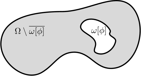
Figure 1: The sets $\Omega\setminus\overline{\omega[\phi]}$ and $\omega[\phi]$.

We also note that the identity function $\mathrm{id}_{\partial\omega}$ of $\partial\omega$ belongs to $\mathcal{A}^{\Omega}_{\partial\omega}$ and, for convenience, we set

$$\phi_{0}:=\mathrm{id}_{\partial\omega}.$$

Accordingly,

$$\Omega\setminus\overline{\omega[\phi_{0}]}=\Omega\setminus\overline{\omega}\,.$$

We observe that $\partial(\Omega\setminus\overline{\omega[\phi]})$ has two connected components: $\partial\Omega$ that remains fixed, and $\partial\omega[\phi]$ that depends on $\phi$. To define the boundary conditions on $\partial(\Omega\setminus\overline{\omega[\phi]})$ we will use two functions $G$ and $f$ such that:

$$\begin{split}&G\in C^{0}([0,T]\times\partial\omega\times\mathbb{R})\,,\quad\quad{G(0,x,0)=0}\quad\text{for all }x\in\partial\omega\,,\\ &\text{and the function}\ [0,T]\times\partial\omega\ni(t,x)\mapsto G(t,x,u(x,t))\ \text{belongs to $C^{\frac{\alpha}{2};\alpha}([0,T]\times\partial\omega)$}\\ &\text{for all $u\in C^{\frac{\alpha}{2};\alpha}([0,T]\times\partial\omega)$}\,,\\ &f\in C_{0}^{\frac{\alpha}{2};\alpha}([0,T]\times\partial\Omega).\end{split}$$ (4)

The function $G$ determines the nonlinear Robin-type condition on the inner boundary $[0,T]\times\phi(\partial\omega)$, while $f$ serves as the Neumann datum on the outer boundary $[0,T]\times\partial\Omega$ (see Section 2 for the definition of $C_{0}^{\frac{\alpha}{2};\alpha}([0,T]\times\partial\Omega)$).

Then we consider the following nonlinear mixed boundary value problem for a function $u\in C_{0}^{\frac{1+\alpha}{2};1+\alpha}([0,T]\times(\overline{\Omega}\setminus\omega[\phi]))$:

$$\begin{cases}\partial_{t}u-\Delta u=0&\quad\text{in }]0,T]\times(\Omega\setminus\overline{\omega[\phi]}),\\ \frac{\partial}{\partial\nu_{\Omega}}u(t,x)=f(t,x)&\quad\forall(t,x)\in[0,T]\times\partial\Omega,\\ \frac{\partial}{\partial{\nu_{\omega[\phi]}}}u(t,x)=G(t,\phi^{(-1)}(x),u(t,x))&\quad\forall(t,x)\in[0,T]\times\partial\omega[\phi],\\ u(0,\cdot)=0&\quad\text{in }\overline{\Omega}\setminus\omega[\phi],\end{cases}$$ (5)

where $\nu_{\Omega}$ and ${\nu_{\omega[\phi]}}$ respectively denote the outward unit normal vector field to $\partial\Omega$ and to $\partial\omega[\phi]=\phi(\partial\omega)$.

Our goal is now as follows: Under suitable assumptions, which include the existence of a solution $u_{0}$ of (5) for $\phi=\phi_{0}$, we aim to establish the existence of solutions $u_{\phi}$ for $\phi$ sufficiently close to the identity. This scenario corresponds to the case where the perturbed hole $\omega[\phi]$ is close to $\omega$. Subsequently, we will demonstrate that the map associating $\phi$ with $u_{\phi}$ is smooth and that the family of solutions $\{u_{\phi}\}_{\phi}$ is locally unique in a sense that will be clarified later on. Finally, in the linear case, we will show the smoothness of the “Neumann-to-Dirichlet” operator upon the shape parameter $\phi$ and the boundary condition.

The paper is organized as follows: Section 2 provides preliminaries on parabolic Schauder spaces and potential theory for the heat equation. In Section 3, we transform problem (5) into an equivalent nonlinear system of integral equations, which we analyze using the Implicit Function Theorem. Additionally, we present our main results on the smoothness of the “domain-to-solution” map (Theorem 3.8) and on the local uniqueness of the family of solutions $\{u_{\phi}\}_{\phi}$ (Proposition 3.9). Finally, some remarks on the linear case in Section 4 conclude the paper.

2 Preliminaries

In this section, we provide some preliminaries, particularly focusing on the potential theory for the heat equation. In the subsequent sections, we will utilize the single layer potential to convert problem (5) into a system of integral equations, which we will then analyze using the Implicit Function Theorem.

We begin by recalling the definition of parabolic Schauder spaces. Let $\alpha\in\mathopen{]}0,1[$, $T>0$ and $\Omega$ be an open subset of $\mathbb{R}^{n}$. Then $C^{\frac{\alpha}{2};\alpha}([0,T]\times\overline{\Omega})$ denotes the space of bounded continuous functions $u$ from $[0,T]\times\overline{\Omega}$ to $\mathbb{R}$ such that

$$\|u\|_{C^{\frac{\alpha}{2};\alpha}([0,T]\times\overline{\Omega})}:= \sup_{[0,T]\times\overline{\Omega}}|u|+\sup_{\begin{subarray}{c}t_{1},t_{2}\in[0,T]\\ t_{1}\neq t_{2}\end{subarray}}\,\sup_{x\in\overline{\Omega}}\frac{|u(t_{1},x)-u(t_{2},x)|}{|t_{1}-t_{2}|^{\frac{\alpha}{2}}}$$

$$+\sup_{t\in[0,T]}\,\sup_{\begin{subarray}{c}x_{1},x_{2}\in\overline{\Omega}\\ x_{1}\neq x_{2}\end{subarray}}\frac{|u(t,x_{1})-u(t,x_{2})|}{|x_{1}-x_{2}|^{\alpha}}<+\infty.$$

Also, $C^{\frac{1+\alpha}{2};1+\alpha}([0,T]\times\overline{\Omega})$ denotes the space of bounded continuous functions $u$ from $[0,T]\times\overline{\Omega}$ to $\mathbb{R}$ which are continuously differentiable with respect to the space variables and such that

$$\|u\|_{C^{\frac{1+\alpha}{2};1+\alpha}([0,T]\times\overline{\Omega})}:= \sup_{[0,T]\times\overline{\Omega}}|u|+\sum_{i=1}^{n}\|\partial_{x_{i}}u\|_{C^{\frac{\alpha}{2};\alpha}([0,T]\times\overline{\Omega})}$$

$$+\sup_{\begin{subarray}{c}t_{1},t_{2}\in[0,T]\\ t_{1}\neq t_{2}\end{subarray}}\,\sup_{x\in\overline{\Omega}}\frac{|u(t_{1},x)-u(t_{2},x)|}{|t_{1}-t_{2}|^{\frac{1+\alpha}{2}}}<+\infty.$$

If $\Omega$ is an open subset of $\mathbb{R}^{n}$ of class $C^{1,\alpha}$, we can use the local parametrization of $\partial\Omega$ to define the space $C^{\frac{1+\alpha}{2};1+\alpha}([0,T]\times\partial\Omega)$ in the natural way. In a similar way, we can define the spaces $C^{j,\alpha}(\mathcal{M})$ and $C^{\frac{j+\alpha}{2};j+\alpha}([0,T]\times\mathcal{M})$, $j\in\{0,1\}$ on a manifold $\mathcal{M}$ of class $C^{j,\alpha}$ imbedded in $\mathbb{R}^{n}$ (see [12, Appendix A]). In essence, a function of class $C^{\frac{j+\alpha}{2};j+\alpha}$ is $\left(\frac{j+\alpha}{2}\right)$-Hölder continuous in the time variable, and $(j,\alpha)$-Schauder regular in the space variable.

We use the subscript $0$ to denote a subspace consisting of functions that are zero at $t=0$. Namely,

$${C_{0}^{\frac{\alpha}{2};\alpha}([0,T]\times\overline{\Omega})}:=\Big{\{}u\in{C^{\frac{\alpha}{2};\alpha}([0,T]\times\overline{\Omega})}\,:\,u(0,x)=0\quad\forall x\in\Omega\Big{\}}.$$

Then the spaces $C_{0}^{\frac{j+\alpha}{2};j+\alpha}([0,T]\times\overline{\Omega})$, $C_{0}^{\frac{j+\alpha}{2};j+\alpha}([0,T]\times\partial\Omega)$ and $C_{0}^{\frac{j+\alpha}{2};j+\alpha}([0,T]\times\mathcal{M})$ with $j\in\{0,1\}$ are similarly defined.

For functions in parabolic Schauder spaces, the partial derivative $D_{x}$ with respect to the space variable $x$ will be denoted by the gradient $\nabla$, while we will maintain the notation $\partial_{t}$ for the derivative with respect to the time variable $t$.

For a comprehensive introduction to parabolic Schauder spaces we refer the reader to classical monographs on the field, for example Ladyženskaja, Solonnikov, and Ural’ceva [24, Chapter 1] (see also [26, 27] for more references).

In our boundary value problem, the nonlinear Robin condition is defined through a superposition operator associated with the function $G$. Therefore, if $\omega$ is as in (1), we now introduce a notation for such operators: If $G$ is a function from $[0,T]\times\partial\omega\times\mathbb{R}$ to $\mathbb{R}$, then we denote by $\mathcal{N}_{G}$ the nonlinear superposition operator that maps a function $u$ from $[0,T]\times\partial\omega$ to the function $\mathcal{N}_{G}(u)$ defined by

$$\mathcal{N}_{G}(u)(t,x):=G(t,x,u(t,x))\quad\text{for all }(t,x)\in[0,T]\times\partial\omega.$$

Here, the letter “$\mathcal{N}$” stands for “Nemytskii operator.”

Now we turn to present some well-known facts on the single layer heat potential. For proofs and detailed references we refer to Ladyženskaja, Solonnikov, and Ural’ceva [24, Chapter 4].

First of all, since layer potentials are integral operators whose kernel is a fundamental solution or its derivatives, we define the function $S_{n}:\mathbb{R}^{1+n}\setminus\{(0,0)\}\to\mathbb{R}$ by

$$S_{n}(t,x):=\left\{\begin{array}[]{ll}\frac{1}{(4\pi t)^{\frac{n}{2}}}e^{-\frac{|x|^{2}}{4t}}&{\mathrm{if}}\ (t,x)\in\mathopen{]}0,+\infty[\times{\mathbb{R}}^{n}\,,\\ 0&{\mathrm{if}}\ (t,x)\in(\mathopen{]}-\infty,0]\times{\mathbb{R}}^{n})\setminus\{(0,0)\}.\end{array}\right.$$

It is well known that $S_{n}$ is a fundamental solution of the heat operator $\partial_{t}-\Delta$ in $\mathbb{R}^{1+n}\setminus\{(0,0)\}$.

We are now in the position to introduce the single layer heat potential. Let $\alpha\in\mathopen{]}0,1[$ and $T>0$. Now let $\Omega$ be an open bounded subset of $\mathbb{R}^{n}$ of class $C^{1,\alpha}$. For a density $\mu\in L^{\infty}\big{(}[0,T]\times\partial\Omega\big{)}$, the single layer heat potential is defined as

$$v_{\Omega}[\mu](t,x):=\int_{0}^{t}\int_{\partial\Omega}S_{n}(t-\tau,x-y)\mu(\tau,y)\,d\sigma_{y}d\tau\quad\forall\,(t,x)\in[0,T]\times\mathbb{R}^{n}.$$

Moreover, we set

$$V_{\partial\Omega}[\mu]:=v_{\Omega}[\mu]_{|[0,T]\times\partial\Omega}$$

and

$$W^{*}_{\partial\Omega}[\mu](t,x):=\int_{0}^{t}\int_{\partial\Omega}\frac{\partial}{\partial\nu_{\Omega}(x)}S_{n}(t-\tau,x-y)\mu(\tau,y)\,d\sigma_{y}d\tau\quad\forall\,(t,x)\in[0,T]\times\partial\Omega\,.$$

The map $V_{\partial\Omega}[\mu]$ is the trace of the single layer heat potential on $[0,T]\times\partial\Omega$, whereas the map $W^{*}_{\partial\Omega}[\mu]$ is associated with the normal derivative of the single layer heat potential on $[0,T]\times\partial\Omega$ (see Theorem 2.1 (iii) below).

Layer heat potentials enjoy properties similar to those of their standard elliptic counterpart. We collect those related to the single layer potential in the following theorem.

Theorem 2.1.

Let $\alpha\in\mathopen{]}0,1[$ and $T>0$. Let $\Omega$ be a bounded open subset of $\mathbb{R}^{n}$ of class $C^{1,\alpha}$. Then the following statements hold.

• Let $\mu\in L^{\infty}([0,T]\times\partial\Omega)$. Then $v_{\Omega}[\mu]$ is continuous and $v_{\Omega}[\mu]\in C^{\infty}(]0,T[\times(\mathbb{R}^{n}\setminus\partial\Omega))$. Moreover $v_{\Omega}[\mu]$ solves the heat equation in $]0,T]\times(\mathbb{R}^{n}\setminus\partial\Omega)$.

• Let $v_{\Omega}^{+}[\mu]$ and $v_{\Omega}^{-}[\mu]$ denote the restrictions of $v_{\Omega}[\mu]$ to $[0,T]\times\overline{\Omega}$ and to $[0,T]\times\overline{\Omega^{-}}$, respectively. Then, the map from $C_{0}^{\frac{\alpha}{2};\alpha}([0,T]\times\partial\Omega)$ to $C_{0}^{\frac{1+\alpha}{2};1+\alpha}([0,T]\times\overline{\Omega})$ that takes $\mu$ to $v_{\Omega}^{+}[\mu]$ is linear and continuous. If $R>0$ is such that $\overline{\Omega}$ is contained in the ball $B(0,R)$ of center $0$ and radius $R$, then the map from $C_{0}^{\frac{\alpha}{2};\alpha}([0,T]\times\partial\Omega)$ to $C_{0}^{\frac{1+\alpha}{2};1+\alpha}([0,T]\times(\overline{B(0,R)}\setminus\Omega^{-}))$ that takes $\mu$ to $v_{\Omega}^{-}[\mu]_{|[0,T]\times(\overline{B(0,R)}\setminus\Omega^{-})}$ is also linear and continuous.

• Let $\mu\in C_{0}^{\frac{\alpha}{2};\alpha}([0,T]\times\partial\Omega)$. Then the following jump relations hold:

  $$\frac{\partial}{\partial\nu_{\Omega}}v_{\Omega}^{\pm}[\mu](t,x)=\pm\frac{1}{2}\mu(t,x)+W_{\partial\Omega}^{*}[\mu](t,x),$$

  for all $(t,x)\in[0,T]\times\partial\Omega$.

• The operator $V_{\partial\Omega}$ is an isomorphism from $C_{0}^{\frac{\alpha}{2};\alpha}([0,T]\times\partial\Omega)$ to $C_{0}^{\frac{1+\alpha}{2};1+\alpha}([0,T]\times\partial\Omega)$.

Proof.

For the proof of points (i)–(iii) we refer, for instance, to [12, 26, 27]. For the proof of (iv), one can simplify the argument of the proof of Brown [3, Prop. 6.2] (which deals with the more involved case of Lipschitz domains) in combination with the regularity results for layer potential operators in Schauder spaces of [26, 27]. For invertibility results of the trace of the single layer potential for the heat equation, see also Costabel [8, Corollary 3.13] and Brown [4, Theorem 4.18]. ∎

Fredholm theory is an important tool for analyzing the integral equations associated with the boundary behavior of layer potentials and their normal derivatives. To apply this theory, we need some compactness results on the embedding of parabolic Schauder spaces, which we state in the following Proposition 2.2. The proof of this proposition is well-known and relies on the Ascoli-Arzelà Theorem.

Proposition 2.2.

Let $\alpha\in\mathopen{]}0,1[$ and $T>0$. Let $\Omega$ be a bounded open subset of $\mathbb{R}^{n}$ of class $C^{1,\alpha}$. Then, the embeddings of $C_{0}^{\frac{\alpha}{2};\alpha}([0,T]\times\partial\Omega)$ into $C_{0}^{\frac{\gamma}{2};\gamma}([0,T]\times\partial\Omega)$ for any $\gamma\in[0,\alpha[$ and of $C_{0}^{\frac{1+\alpha}{2};1+\alpha}([0,T]\times\partial\Omega)$ into $C_{0}^{\frac{\alpha}{2};\alpha}([0,T]\times\partial\Omega)$ are compact.

From Proposition 2.2, combined with Theorem 2.1 (iv) and [27, Theorem 4.6], we readily derive the following Theorem 2.3 on the mapping and compactness properties of the operators $V_{\partial\Omega}$ and $W^{\ast}_{\partial\Omega}$.

Theorem 2.3.

Let $\alpha\in\mathopen{]}0,1[$ and $T>0$. Let $\Omega$ be a bounded open subset of $\mathbb{R}^{n}$ of class $C^{1,\alpha}$. Then, the operators $V_{\partial\Omega}$ and $W^{*}_{\partial\Omega}$ are compact from $C_{0}^{\frac{\alpha}{2};\alpha}([0,T]\times\partial\Omega)$ to itself.

Problem (5) is defined in a perforated domain, which is a connected set obtained by removing a part of a larger domain. We will need some results for functions defined in these specific types of sets. Therefore, in the remaining part of this section, we focus on perforated domains. We consider the following assumption:

$$\begin{split}&\mbox{$\Omega$ and $\tilde{\omega}$ are bounded open connected subsets of $\mathbb{R}^{n}$ of class $C^{1,\alpha}$,}\\ &\mbox{with connected exteriors {$\Omega^{-}:=\mathbb{R}^{n}\setminus\overline{\Omega}$ and $\tilde{\omega}^{-}:=\mathbb{R}^{n}\setminus\overline{\tilde{\omega}}$} and such that $\overline{\tilde{\omega}}\subseteq\Omega$}.\end{split}$$ (6)

By Theorem 2.1 (iv) and by the uniqueness of the solution of the Dirichlet problem for the heat equation, we deduce the following Lemma 2.4, where we see that solutions of the heat equation that are in $C_{0}^{\frac{1+\alpha}{2};1+\alpha}([0,T]\times(\overline{\Omega}\setminus\tilde{\omega}))$ can be represented as a sum of single layer potentials.

Lemma 2.4.

Let $\alpha\in\mathopen{]}0,1[$ and $T>0$. Let $\Omega$ and $\tilde{\omega}$ be as in assumption (6). Then the map from $C_{0}^{\frac{\alpha}{2};\alpha}([0,T]\times\partial\Omega)\times C_{0}^{\frac{\alpha}{2};\alpha}([0,T]\times\partial\tilde{\omega})$ to the space

$$\left\{u\in C_{0}^{\frac{1+\alpha}{2};1+\alpha}([0,T]\times(\overline{\Omega}\setminus\tilde{\omega}))\,:\,\partial_{t}u-\Delta u=0\quad\text{in }{\mathopen{]}0,T]}\times{(\Omega\setminus\overline{\tilde{\omega}})}\right\}$$

that takes a pair $(\mu,\eta)$ to the function

$${u_{\Omega,\tilde{\omega}}[\mu,\eta]:=}(v^{+}_{\Omega}[\mu]+v^{-}_{\tilde{\omega}}[\eta])_{|[0,T]\times(\overline{\Omega}\setminus\tilde{\omega})}$$ (7)

is a bijection.

To apply the Implicit Function Theorem, we need to examine a linearization of problem (5), i.e., a linear mixed Neumann-Robin boundary value problem. For this, we need the following uniqueness result, whose proof follows, for example, from Liebermann [29, Corollary 5.4] (see also Friedman [16, Lemma 2, p. 146] and Ladyzhenskaja, Solonnikov, and Ural’ceva [24, Chapter 4, §5]).

Lemma 2.5.

Let $\alpha\in\mathopen{]}0,1[$ and $T>0$. Let $\Omega$ and $\tilde{\omega}$ be as in assumption (6). Let $\beta\in C^{\frac{\alpha}{2};\alpha}([0,T]\times\partial\tilde{\omega})$. Then the unique solution in $C_{0}^{\frac{1+\alpha}{2};1+\alpha}([0,T]\times(\overline{\Omega}\setminus\tilde{\omega}))$ of problem

$$\begin{cases}\partial_{t}u-\Delta u=0&\quad\text{in }\mathopen{]}0,T]\times(\Omega\setminus\overline{\tilde{\omega}}),\\ \frac{\partial}{\partial\nu_{\Omega}}u(t,x)=0&\quad\forall(t,x)\in[0,T]\times\partial\Omega,\\ {\frac{\partial}{\partial\nu_{\tilde{\omega}}}u}(t,x)-\beta(t,x)u(t,x)=0&\quad\forall(t,x)\in[0,T]\times\partial\tilde{\omega},\\ u(0,\cdot)=0&\quad\text{in }\overline{\Omega}\setminus\tilde{\omega},\end{cases}$$ (8)

is $u=0$.

We conclude this section with the following proposition, where we investigate an auxiliary boundary operator, $\mathcal{J}_{\beta}$, associated with the linear Neumann-Robin boundary value problem (8). We are going to use $\mathcal{J}_{\beta}$ to analyze the integral formulation of problem (5).

Proposition 2.6.

Let $\alpha\in\mathopen{]}0,1[$ and $T>0$. Let $\Omega$ and $\tilde{\omega}$ be as in assumption (6). Let $\beta\in C^{\frac{\alpha}{2};\alpha}([0,T]\times\partial\tilde{\omega})$. Let $\mathcal{J}_{\beta}=(\mathcal{J}_{\beta,1},\mathcal{J}_{\beta,2})$ be the map from $C_{0}^{\frac{\alpha}{2};\alpha}([0,T]\times\partial\Omega)\times C_{0}^{\frac{\alpha}{2};\alpha}([0,T]\times\partial\tilde{\omega})$ to itself that takes a pair $(\mu,\eta)$ to the pair $\mathcal{J}_{\beta}[\mu,\eta]:=(\mathcal{J}_{\beta,1}[\mu,\eta],\mathcal{J}_{\beta,2}[\mu,\eta])$ defined by

$$\mathcal{J}_{\beta,1}[\mu,\eta] :=\left(\frac{1}{2}I+W^{\ast}_{\partial\Omega}\right)[\mu]+\nu_{\Omega}\cdot\nabla v^{-}_{\tilde{\omega}}[\eta]_{|[0,T]\times\partial\Omega},$$ (9)

$$\mathcal{J}_{\beta,2}[\mu,\eta] :=\left(-\frac{1}{2}I+W^{\ast}_{\partial\tilde{\omega}}\right)[\eta]+\nu_{\tilde{\omega}}\cdot\nabla v^{+}_{\Omega}[\mu]_{|[0,T]\times\partial\tilde{\omega}}-\beta(v^{+}_{\Omega}[\mu]_{|[0,T]\times\partial\tilde{\omega}}+V_{\partial\tilde{\omega}}[\eta]).$$

Then $\mathcal{J}_{\beta}$ is a linear homeomorphism from $C_{0}^{\frac{\alpha}{2};\alpha}([0,T]\times\partial\Omega)\times C_{0}^{\frac{\alpha}{2};\alpha}([0,T]\times\partial\tilde{\omega})$ to itself.

Proof.

Let $\bar{\mathcal{J}}:=(\bar{\mathcal{J}}_{1},\bar{\mathcal{J}}_{2})$ be the linear operator from $C_{0}^{\frac{\alpha}{2};\alpha}([0,T]\times\partial\Omega)\times C_{0}^{\frac{\alpha}{2};\alpha}([0,T]\times\partial\tilde{\omega})$ to itself defined by

$$\bar{\mathcal{J}}_{1}[\mu,\eta]:=\frac{1}{2}\mu,\quad\bar{\mathcal{J}}_{2}[\mu,\eta]:=-\frac{1}{2}\eta,$$

for all $(\mu,\eta)\in C_{0}^{\frac{\alpha}{2};\alpha}([0,T]\times\partial\Omega)\times C_{0}^{\frac{\alpha}{2};\alpha}([0,T]\times\partial\tilde{\omega})$. Clearly $\bar{\mathcal{J}}$ is a linear homeomorphism.

Moreover, by Theorem 2.3, by the results of [12, Lemmas A.2, A.3] on non-autonomous composition operators and on time-dependent integral operators with non-singular kernels, and by the compactness of the embeddings of parabolic Schauder spaces of Theorem 2.2, we deduce that the map from $C_{0}^{\frac{\alpha}{2};\alpha}([0,T]\times\partial\Omega)\times C_{0}^{\frac{\alpha}{2};\alpha}([0,T]\times\partial\tilde{\omega})$ to itself that takes a pair $(\mu,\eta)$ to the pair $\mathcal{J}^{C}_{\beta}[\mu,\eta]{=(\mathcal{J}^{C}_{\beta,1}[\mu,\eta],\mathcal{J}^{C}_{\beta,1}[\mu,\eta])}$ defined by

$$\mathcal{J}^{C}_{\beta,1}[\mu,\eta] :=W^{\ast}_{\partial\Omega}[\mu]+\nu_{\Omega}\cdot\nabla v^{-}_{\tilde{\omega}}[\eta]_{|[0,T]\times\partial\Omega} \text{on }[0,T]\times\partial\Omega,$$

$$\mathcal{J}^{C}_{\beta,2}[\mu,\eta] :=W^{\ast}_{\partial\tilde{\omega}}[\eta]+\nu_{\tilde{\omega}}\cdot\nabla v^{+}_{\Omega}[\mu]_{|[0,T]\times\partial\tilde{\omega}}-\beta(v^{+}_{\Omega}[\mu]_{|[0,T]\times\partial\tilde{\omega}}+V_{\partial\tilde{\omega}}[\eta]) \text{on }[0,T]\times\partial\tilde{\omega},$$

is compact. Since compact perturbations of linear homeomorphisms are Fredholm operators of index $0$, we have that $\mathcal{J}_{\beta}=\bar{\mathcal{J}}+\mathcal{J}^{C}_{\beta}$ is a Fredholm operator of index $0$. Therefore, in order to complete the proof, it suffices to prove that $\mathcal{J}_{\beta}$ is injective. Thus, we now assume that $(\mu,\eta)\in C_{0}^{\frac{\alpha}{2};\alpha}([0,T]\times\partial\Omega)\times C_{0}^{\frac{\alpha}{2};\alpha}([0,T]\times\partial\tilde{\omega})$ is such that

$$\mathcal{J}_{\beta}[\mu,\eta]=(0,0).$$ (10)

Then, by the jump formulas of Theorem 2.1 (iii) and by (10), we deduce that the function ${u_{\Omega,\tilde{\omega}}}[\mu,\eta]$ defined by (7) is a solution of the boundary value problem (8). Then by Lemma 2.5, we have that ${u_{\Omega,\tilde{\omega}}}[\mu,\eta]=0$, which implies $(\mu,\eta)=(0,0)$, by the uniqueness of the representation provided by Lemma 2.4. ∎

3 The perturbed nonlinear mixed problem (5)

We now take into consideration the perturbed problem (5). As mentioned, we aim to demonstrate, under suitable conditions, the existence of solutions $u_{\phi}$ for $\phi$ close to the identity and show that the “domain-to-solution” map $\phi\mapsto u_{\phi}$ is smooth.

The first step is transforming the nonlinear problem (5) into a nonlinear system of integral equations.

Let $\alpha\in\mathopen{]}0,1[$, $T>0$ and let $\Omega$, $\omega$ be as in (1). Let $G$, $f$ be as in (4). We note that the assumptions in (4) on $G$ imply that $\mathcal{N}_{G}$ maps $C_{0}^{\frac{\alpha}{2};\alpha}([0,T]\times\partial\omega)$ to itself.

Then let $\mathcal{M}=(\mathcal{M}_{1},\mathcal{M}_{2})$ be the map from $\mathcal{A}^{\Omega}_{\partial\omega}\times C_{0}^{\frac{\alpha}{2};\alpha}([0,T]\times\partial\Omega)\times C_{0}^{\frac{\alpha}{2};\alpha}([0,T]\times\partial\omega)$ to $C_{0}^{\frac{\alpha}{2};\alpha}([0,T]\times\partial\Omega)\times C_{0}^{\frac{\alpha}{2};\alpha}([0,T]\times\partial\omega)$ defined by

$$\mathcal{M}_{1}[\phi,\mu,\eta] :=\left(\frac{1}{2}I+W^{\ast}_{\partial\Omega}\right)[\mu]+\nu_{\Omega}\cdot\nabla v^{-}_{\omega[\phi]}[\eta\circ(\phi^{T})^{(-1)}]-f,$$ (11)

$$\mathcal{M}_{2}[\phi,\mu,\eta] :=\left(-\frac{1}{2}I+W^{\ast}_{\partial\omega[\phi]}\right)[\eta\circ(\phi^{T})^{(-1)}]\circ\phi^{T}+\left({\nu_{\omega[\phi]}}\circ\phi\right)\cdot\nabla v^{+}_{\Omega}[\mu]\circ\phi^{T}$$

$$\quad-\mathcal{N}_{G}\Big{(}v^{+}_{\Omega}[\mu]_{|[0,T]\times\partial\omega[\phi]}\circ\phi^{T}+V_{\partial\omega[\phi]}[\eta\circ\phi^{(-1)}]\circ\phi^{T}\Big{)},$$

for all $(\phi,\mu,\eta)\in\mathcal{A}^{\Omega}_{\partial\omega}\times C_{0}^{\frac{\alpha}{2};\alpha}([0,T]\times\partial\Omega)\times C_{0}^{\frac{\alpha}{2};\alpha}([0,T]\times\partial\omega)$. Here, we have used the following notation, which will also be adopted throughout the remainder of the paper: If $A$ is a subset of $\mathbb{R}^{n}$, $T>0$ and $h$ is a map from $A$ to $\mathbb{R}^{n}$, we denote by $h^{T}$ the map from $[0,T]\times A$ to $[0,T]\times\mathbb{R}^{n}$ defined by

$$h^{T}(t,x):=(t,h(x))\quad\forall(t,x)\in[0,T]\times A.$$

From the definition of $\mathcal{M}$, we readily deduce the following:

Proposition 3.1.

Let $\alpha\in\mathopen{]}0,1[$ and $T>0$. Let $\Omega$, $\omega$ be as in (1). Let $G$, $f$ be as in (4). Let

$$(\phi,\mu,\eta)\in\mathcal{A}^{\Omega}_{\partial\omega}\times C_{0}^{\frac{\alpha}{2};\alpha}([0,T]\times\partial\Omega)\times C_{0}^{\frac{\alpha}{2};\alpha}([0,T]\times\partial\omega).$$

Then the function

$$u_{\Omega,\omega[\phi]}[\mu,\eta\circ(\phi^{T})^{(-1)}]:=(v^{+}_{\Omega}[\mu]+v^{-}_{\omega[\phi]}[\eta\circ(\phi^{T})^{(-1)}])_{|[0,T]\times(\overline{\Omega}\setminus{\omega[\phi]})}$$

(cf. (7)) is a solution of problem (5) if and only if

$$\mathcal{M}[\phi,\mu,\eta]=(0,0).$$ (12)

Proof.

By the regularity of $\phi\in\mathcal{A}^{\Omega}_{\partial\omega}$ we have that if $(\mu,\eta)\in C_{0}^{\frac{\alpha}{2};\alpha}([0,T]\times\partial\Omega)\times C_{0}^{\frac{\alpha}{2};\alpha}([0,T]\times\partial\omega)$, then

$$(\mu,\eta\circ(\phi^{T})^{(-1)})\in C_{0}^{\frac{\alpha}{2};\alpha}([0,T]\times\partial\Omega)\times C_{0}^{\frac{\alpha}{2};\alpha}([0,T]\times\phi(\partial\omega)).$$

Moreover, since $\overline{\omega[\phi]}\subseteq\Omega$ (cf. (3)), we can apply Lemma 2.4 with $\tilde{\omega}=\omega[\phi]$. Then, by the jump relations for the single layer potential (cf. Theorem 2.1 (iii)), by a change of variable on $\phi(\partial\omega)$, and by the definition of $\mathcal{M}$ in (11), we deduce that the function

$$u_{\Omega,\omega[\phi]}[\mu,\eta\circ(\phi^{T})^{(-1)}]=(v^{+}_{\Omega}[\mu]+v^{-}_{\omega[\phi]}[\eta\circ(\phi^{T})^{(-1)})_{|[0,T]\times\overline{\Omega}\setminus\omega[\phi]}$$

is a solution of problem (5) if and only if (12) is satisfied. ∎

To carry on our analysis, we will assume the existence of a solution $u_{0}\in C_{0}^{\frac{1+\alpha}{2};1+\alpha}([0,T]\times(\overline{\Omega}\setminus\omega))$ to problem (5) for $\phi=\phi_{0}=\mathrm{id}_{\partial\omega}$. In this paper, we will not explore conditions ensuring the existence of such solution, which can be obtained by several methods. For example, one may adapt the argument from [14] and impose a growth condition on $G$ to apply the Leray-Schauder Fixed Point Theorem. For a discussion on nonlinear boundary value problems for parabolic equations, readers may consult Friedman [16, Chapter 7].

Combining Lemma 2.4 and Proposition 3.1, we can readily see that such solution $u_{0}$ can be expressed as a sum of single layer potentials. Namely, we have the following:

Proposition 3.2.

Let $\alpha\in\mathopen{]}0,1[$ and $T>0$. Let $\Omega$, $\omega$ be as in (1). Let $G$, $f$ be as in (4). Let $\phi_{0}:=\mathrm{id}_{\partial\omega}$. Assume that $u_{0}\in C_{0}^{\frac{1+\alpha}{2};1+\alpha}([0,T]\times(\overline{\Omega}\setminus\omega))$ is a solution of

$$\begin{cases}\partial_{t}u-\Delta u=0&\quad\text{in }]0,T]\times(\Omega\setminus\overline{\omega}),\\ \frac{\partial}{\partial\nu_{\Omega}}u(t,x)=f(t,x)&\quad\forall(t,x)\in[0,T]\times\partial\Omega,\\ {\frac{\partial}{\partial\nu_{\omega}}u(t,x)=G(t,x,u(t,x))}&\quad\forall(t,x)\in[0,T]\times\partial\omega,\\ u(0,\cdot)=0&\quad\text{in }\overline{\Omega}\setminus\omega\,.\end{cases}$$

Then there exists a unique pair $(\mu_{0},\eta_{0})\in C_{0}^{\frac{\alpha}{2};\alpha}([0,T]\times\partial\Omega)\times C_{0}^{\frac{\alpha}{2};\alpha}([0,T]\times\partial\omega)$ such that

$$u_{0}=u_{\Omega,\omega[\phi_{0}]}[\mu_{0},\eta_{0}\circ(\phi_{0}^{T})^{(-1)}]{=u_{\Omega,\omega}[\mu_{0},\eta_{0}]}\,.$$

In particular,

$$\mathcal{M}[\phi_{0},\mu_{0},\eta_{0}]=(0,0)\,.$$

According to Proposition 3.1, the analysis of problem (5) is reduced to that of equation (12), which we intend to study using the Implicit Function Theorem for $C^{\infty}$ maps in Banach spaces (cf. Deimling [15, Theorem 15.1 & Corollary 15.1]). Consequently, we need to examine the regularity of the map $\mathcal{M}$. If we were dealing with an elliptic equation, we would expect an analyticity result at this point (see, e.g., [25, 28]). However, this is not the case for the heat equation.

Indeed, in the definition of $\mathcal{M}$, we have the pull-back of integral operators associated with heat layer potentials. By the results of [12] we only know that these are of class $C^{\infty}$. This crucial difference from the elliptic case obstructs the proof of analyticity results and reflects the regularity of the fundamental solution $S_{n}$, which is analytic in $\mathbb{R}^{n}\setminus\{0\}$ in the case of elliptic operators but only $C^{\infty}$ on $\mathbb{R}^{1+n}\setminus\{(0,0)\}$ for the heat equation.

In the definition of $\mathcal{M}$ we also have a superposition operator associated with the function $G$. To handle this, we will assume that

$$\mathcal{N}_{G} C^{\infty} C^{\frac{\alpha}{2};\alpha}([0,T]\times\partial\omega)$$ is of class from to itself. (13)

For example, a suitable choice of $G$ ensuring that $\mathcal{N}_{G}$ is of class $C^{\infty}$ from $C^{\frac{\alpha}{2};\alpha}([0,T]\times\partial\omega)$ to itself is any polynomial function $G(t,\xi)=a_{0}(t)+a_{1}(t)\xi+\ldots+a_{k}(t)\xi^{k}$ with $a_{0}(0)=0$. We note that by assumptions (4) and (13) and by computing the differentials of $\mathcal{N}_{G}$ (as it is done for example in Valent [37, Proof of Thm. 4.1]), one verifies that $\mathcal{N}_{G}$ is of class $C^{\infty}$ also from the function space $C^{\frac{\alpha}{2};\alpha}_{0}([0,T]\times\partial\omega)$, consisting of functions that are zero at $t=0$, to itself.

Finally, to study the regularity of the map $\mathcal{M}$, we also need the following technical lemma on the smoothness of certain maps related to the change of variables in integrals and to the pull-back of the outer normal field. A proof can be found in Lanza de Cristoforis and Rossi [28, p. 166] and Lanza de Cristoforis [25, Prop. 1].

Lemma 3.3.

Let $\alpha\in\mathopen{]}0,1[$. Let $\omega$ be an open bounded connected subset of $\mathbb{R}^{n}$ of class $C^{1,\alpha}$ with connected exterior $\mathbb{R}^{n}\setminus\overline{\omega}$. Let $\mathcal{A}_{\partial\omega}$ be as in (2). Then the following hold.

• For each $\phi\in\mathcal{A}_{\partial\omega}$ there exists a unique $\tilde{\sigma}_{n}[\phi]\in C^{0,\alpha}(\partial\omega)$ such that

  $$\int_{\phi(\partial\omega)}f(y)\,d\sigma_{y}=\int_{\partial\omega}f(\phi(s))\,\tilde{\sigma}_{n}[\phi](s)\,d\sigma_{s}\quad\forall f\in L^{1}(\phi(\partial\omega)).$$

  Moreover, $\tilde{\sigma}_{n}[\phi]>0$ and the map taking $\phi$ to $\tilde{\sigma}_{n}[\phi]$ is real analytic from $\mathcal{A}_{\partial\omega}$ to $C^{0,\alpha}(\partial\omega)$.

• The map from $\mathcal{A}_{\partial\omega}$ to $C^{0,\alpha}(\partial\omega)$ that takes $\phi$ to ${\nu_{\omega[\phi]}}\circ\phi$ is real analytic.

We can now prove that the map $\mathcal{M}$ is of class $C^{\infty}$.

Proposition 3.4.

Let $\alpha\in\mathopen{]}0,1[$ and $T>0$. Let $\Omega$, $\omega$ be as in (1). Let $G$, $f$ be as in (4). Let assumption (13) holds. Then the map $\mathcal{M}$ from $\mathcal{A}^{\Omega}_{\partial\omega}\times C_{0}^{\frac{\alpha}{2};\alpha}([0,T]\times\partial\Omega)\times C_{0}^{\frac{\alpha}{2};\alpha}([0,T]\times\partial\omega)$ to $C_{0}^{\frac{\alpha}{2};\alpha}([0,T]\times\partial\Omega)\times C_{0}^{\frac{\alpha}{2};\alpha}([0,T]\times\partial\omega)$ is of class $C^{\infty}$.

Proof.

We confine to analyze $\mathcal{M}_{2}$. The proof that $\mathcal{M}_{1}$ is smooth follows a similar but simpler argument, which we leave to the reader.

We begin by noting that the map from $\mathcal{A}^{\Omega}_{\partial\omega}\times C_{0}^{\frac{\alpha}{2};\alpha}([0,T]\times\partial\omega)$ to $C_{0}^{\frac{\alpha}{2};\alpha}([0,T]\times\partial\omega)$ that takes a pair $(\phi,\eta)$ to the function of the variables $(t,x)\in[0,T]\times\partial\omega$ defined by

$$\left(-\frac{1}{2}I+W^{\ast}_{\partial\omega[\phi]}\right)[\eta\circ(\phi^{T})^{(-1)}](\phi^{T}(t,x))=-\frac{1}{2}\eta(t,x)+W^{\ast}_{\partial\omega[\phi]}[\eta\circ(\phi^{T})^{(-1)}](\phi^{T}(t,x))$$

is of class $C^{\infty}$, as we can verify by the results on the dependence of heat layer potentials upon perturbation of the support and of the density of [12, Theorem 5.4].

Then we turn to the second term in $\mathcal{M}_{2}$: The map from $\mathcal{A}^{\Omega}_{\partial\omega}\times C_{0}^{\frac{\alpha}{2};\alpha}([0,T]\times\partial\Omega)$ to $C_{0}^{\frac{\alpha}{2};\alpha}([0,T]\times\partial\omega)$ which takes $(\phi,\mu)$ to the function of the variables $(t,x)\in[0,T]\times\partial\omega$ defined by

$${\nu_{\omega[\phi]}}(\phi(x))\cdot\nabla v^{+}_{\Omega}[\mu](t,\phi(x))=\int_{0}^{t}\int_{\partial\Omega}{\nu_{\omega[\phi]}}(\phi(x))\cdot\nabla S_{n}(t-\tau,\phi(x)-y)\mu(\tau,y)\,d\sigma_{y}d\tau$$

is of class $C^{\infty}$ by Lemma 3.3 and by the results of [12, Lemmas A.2, A.3] on non-autonomous composition operators and on time-dependent integral operators with non-singular kernels (notice that $\phi(x)-y\neq 0$ for every $(x,y)\in{\partial\omega\times\partial\Omega}$ thanks to the assumption $\phi\in\mathcal{A}^{\Omega}_{\partial\omega}$, cf. (3)).

Next we consider the argument of $\mathcal{N}_{G}$: The map from $\mathcal{A}^{\Omega}_{\partial\omega}\times C_{0}^{\frac{\alpha}{2};\alpha}([0,T]\times\partial\omega)$ to $C_{0}^{\frac{\alpha}{2};\alpha}([0,T]\times\partial\omega)$ taking a pair $(\phi,\eta)$ to the function

$$V_{\partial\omega[\phi]}[\eta\circ(\phi^{T})^{(-1)}]\circ\phi^{T}$$

is of class $C^{\infty}$ by the results on the dependence of heat layer potentials upon perturbation of the support and of the density of [12, Theorem  5.4] and the map from $\mathcal{A}^{\Omega}_{\partial\omega}\times C_{0}^{\frac{\alpha}{2};\alpha}([0,T]\times\partial\Omega)$ to $C_{0}^{\frac{\alpha}{2};\alpha}([0,T]\times\partial\omega)$ taking a pair $(\phi,\mu)$ to the function of the variables $(t,x)\in[0,T]\times\partial\omega$

$$v^{+}_{\Omega}[\mu](t,\phi(x))=\int_{0}^{t}\int_{\partial\Omega}S_{n}(t-\tau,\phi(x)-y)\mu(\tau,y)\,d\sigma_{y}d\tau$$

is of class $C^{\infty}$ by the results of [12, Lemmas A.2, A.3] on non-autonomous composition operators and on time-dependent integral operators with non-singular kernels (notice again that $\phi(x)-y\neq 0$ for every $(x,y)\in{\partial\omega\times\partial\Omega}$, cf. (3)).

Hence, since composition of $C^{\infty}$ maps is $C^{\infty}$, assumption (13) ensures that the map $\mathcal{A}^{\Omega}_{\partial\omega}\times C_{0}^{\frac{\alpha}{2};\alpha}([0,T]\times\partial\Omega)\times C_{0}^{\frac{\alpha}{2};\alpha}([0,T]\times\partial\omega)$ to $C_{0}^{\frac{\alpha}{2};\alpha}([0,T]\times\partial\omega)$ that takes a triple $(\phi,\mu,\eta)$ to the function

$$\mathcal{N}_{G}\Big{(}v^{+}_{\Omega}[\mu]_{|[0,T]\times\partial\omega[\phi]}\circ\phi^{T}+V_{\partial\omega[\phi]}[\eta\circ(\phi^{T})^{(-1)}]\circ\phi^{T}\Big{)}$$

is of class $C^{\infty}$. Thus, the validity of the statement follows. ∎

By computing the Frechét derivative of $\mathcal{N}_{G}$, we first note that under assumption (13) the partial derivative $\partial_{\xi}G(t_{0},x_{0},\xi_{0})$ of the function $G$ with respect to the third variable exists at any point $(t_{0},x_{0},\xi_{0})\in[0,T]\times\partial\omega\times\mathbb{R}$. Then, using assumption (13) and the standard rules of calculus in Banach spaces, we can derive the following formula for the first-order differential of $\mathcal{N}_{G}$: At any given point $u\in C^{\frac{\alpha}{2};\alpha}([0,T]\times\partial\omega)$, we have

$$d\mathcal{N}_{G}(u)\,.\,h=\mathcal{N}_{\partial_{\xi}G}(u)\,h\qquad\forall h\in C^{\frac{\alpha}{2};\alpha}([0,T]\times\partial\omega),$$

where $\partial_{\xi}G$ denotes the partial derivative of the function $G$ with respect to the third variable (cf. Valent [37, Proof of Thm. 4.1]). We also note that $\mathcal{N}_{\partial_{\xi}G}(u)$ belongs to $C^{\frac{\alpha}{2};\alpha}([0,T]\times\partial\omega)$ for all $u\in C^{\frac{\alpha}{2};\alpha}([0,T]\times\partial\omega)$.

We can now prove the following proposition, where we show that the partial differential of $\mathcal{M}$ with respect to the densities $(\mu,\eta)$ is invertible at $(\phi_{0},\mu_{0},\eta_{0})$. This constitutes an essential step to apply the Implicit Function Theorem to equation (12).

Proposition 3.5.

Let $\alpha\in\mathopen{]}0,1[$ and $T>0$. Let $\Omega$, $\omega$ be as in (1). Let $G$, $f$ be as in (4). Let assumption (13) hold. Let $\phi_{0}$, $u_{0}$, $(\mu_{0},\eta_{0})$ be as in Proposition 3.2. Then the partial differential of $\mathcal{M}$ with respect to $(\mu,\eta)$ evaluated at the point $(\phi_{0},\mu_{0},\eta_{0})$, which we denote by

$$\partial_{(\mu,\eta)}\mathcal{M}[\phi_{0},\mu_{0},\eta_{0}],$$ (14)

is an homeomorphism from $C_{0}^{\frac{\alpha}{2};\alpha}([0,T]\times\partial\Omega)\times C_{0}^{\frac{\alpha}{2};\alpha}([0,T]\times\partial\omega)$ into itself.

Proof.

By standard calculus in Banach spaces, we can verify that the partial differential (14) is the linear and continuous operator from $C_{0}^{\frac{\alpha}{2};\alpha}([0,T]\times\partial\Omega)\times C_{0}^{\frac{\alpha}{2};\alpha}([0,T]\times\partial\omega)$ to itself given by

$$\partial_{(\mu,\eta)}\mathcal{M}_{1}[\phi_{0},\mu_{0},\eta_{0}]\,.\,(\mu,\eta) {=}\left(\frac{1}{2}I+W^{\ast}_{\partial\Omega}\right)[\mu]+{\nu_{\Omega}\cdot\nabla v^{-}_{\omega}[\eta]},$$ (15)

$$\partial_{(\mu,\eta)}\mathcal{M}_{2}[\phi_{0},\mu_{0},\eta_{0}]\,.\,(\mu,\eta) {=}\left(-\frac{1}{2}I+W^{\ast}_{\partial\omega}\right)[\eta]+{\nu_{\omega}}\cdot\nabla v^{+}_{\Omega}[\mu]$$

$$\quad-\mathcal{N}_{\partial_{\xi}G}\Big{(}v^{+}_{\Omega}[\mu_{0}]_{|[0,T]\times\partial\omega}+{V_{\partial\omega}}[\eta_{0}]\Big{)}(v^{+}_{\Omega}[\mu]_{|[0,T]\times\partial\omega}+{V_{\partial\omega}}[\eta]),$$

for all $(\mu,\eta)\in C_{0}^{\frac{\alpha}{2};\alpha}([0,T]\times\partial\Omega)\times C_{0}^{\frac{\alpha}{2};\alpha}([0,T]\times\partial\omega)$. Then, comparing (15) with (9), Proposition 2.6 with the choice

$$\beta:=\mathcal{N}_{\partial_{\xi}G}(v^{+}_{\Omega}[\mu_{0}]_{|[0,T]\times\partial\omega}+{V_{\partial\omega}}[\eta_{0}])$$

implies the validity of the statement. Notice that $\beta\in C^{\frac{\alpha}{2};\alpha}([0,T]\times\partial{\omega})$ by assumption (13). ∎

With Propositions 3.4 and 3.5 we have all the necessary ingredients to apply the Implicit Function Theorem (cf. Deimling [15, Theorem 15.1 & Corollary 15.1]) to equation (12). We obtain the following:

Theorem 3.6.

Let $\alpha\in\mathopen{]}0,1[$ and $T>0$. Let $\Omega$, $\omega$ be as in (1). Let $G$, $f$ be as in (4). Let assumption (13) hold. Let $\phi_{0}$, $u_{0}$, $(\mu_{0},\eta_{0})$ be as in Proposition 3.2. Then, there exist two open neighborhoods $Q_{0}$ of $\phi_{0}$ in $\mathcal{A}^{\Omega}_{\partial\omega}$ and $H_{0}$ of $(\mu_{0},\eta_{0})$ in $C_{0}^{\frac{\alpha}{2};\alpha}([0,T]\times\partial\Omega)\times C_{0}^{\frac{\alpha}{2};\alpha}([0,T]\times\partial\omega)$, and a $C^{\infty}$ map

$$\Lambda:=(\Lambda_{1},\Lambda_{2}):Q_{0}\to H_{0}$$

such that the set of zeros of $\mathcal{M}$ in $Q_{0}\times H_{0}$ coincides with the graph of the function $\Lambda$. In particular,

$$\mathcal{M}[\phi,\Lambda_{1}[\phi],\Lambda_{2}[\phi]]=0\quad\forall\phi\in Q_{0}\,,\qquad\Lambda[\phi_{0}]=(\Lambda_{1}[\phi_{0}],\Lambda_{2}[\phi_{0}])=(\mu_{0},\eta_{0}).$$

Theorem 3.6 yields a family of solutions smoothly depending on $\phi$ for the system of integral equations in (12), which in turn can be used to generate a family of solutions for the equivalent perturbed boundary value problem (5) (cf. Proposition 3.1, see also Proposition 3.2 and Theorem 3.6).

Theorem 3.7.

Let $\alpha\in\mathopen{]}0,1[$ and $T>0$. Let $\Omega$, $\omega$ be as in (1). Let $G$, $f$ be as in (4). Let assumption (13) hold. Let $\phi_{0}$, $u_{0}$, $(\mu_{0},\eta_{0})$ be as in Proposition 3.2. Let $Q_{0}$ and $\Lambda:=(\Lambda_{1},\Lambda_{2})$ be as in Theorem 3.6. For each $\phi\in Q_{0}$, let

$$\begin{split}u_{\phi}&:=u_{\Omega,\omega[\phi]}[\Lambda_{1}[\phi],\Lambda_{2}[\phi]\circ(\phi^{T})^{(-1)}]\\ &=(v^{+}_{\Omega}[\Lambda_{1}[\phi]]+v^{-}_{\omega[\phi]}[\Lambda_{2}[\phi]\circ(\phi^{T})^{(-1)}])_{|[0,T]\times(\overline{\Omega}\setminus{\omega[\phi]})}\end{split}$$

(cf. (7)). Then $u_{\phi}$ is a solution of (5) and $u_{\phi_{0}}=u_{0}$.

In the following theorem, we take a bounded open set $\Omega_{\mathtt{int}}$ such that

$${\overline{\Omega}_{\mathtt{int}}}\subseteq\Omega\setminus\overline{\omega}$$

(see Figure 2) and for $\phi$ close to the identity we show that restriction of the solution $u_{\phi}$ to ${\overline{\Omega}_{\mathtt{int}}}$ depends smoothly on $\phi$.

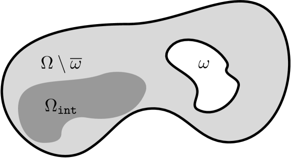
Figure 2: The sets $\omega$, $\Omega\setminus\overline{\omega}$, and $\Omega_{\mathtt{int}}$.

Theorem 3.8.

Let $\alpha\in\mathopen{]}0,1[$ and $T>0$. Let $\Omega$, $\omega$ be as in (1). Let $G$, $f$ be as in (4). Let assumption (13) hold. Let $\phi_{0}$, $u_{0}$, $(\mu_{0},\eta_{0})$ be as in Proposition 3.2. Let $Q_{0}$ and $\Lambda:=(\Lambda_{1},\Lambda_{2})$ be as in Theorem 3.6 and let $\{u_{\phi}\}_{\phi\in Q_{0}}$ be as in Theorem 3.7. Let $\Omega_{\mathtt{int}}$ be a bounded open subset of $\Omega\setminus\overline{\omega}$ such that

$${\overline{\Omega}_{\mathtt{int}}}\subseteq\Omega\setminus\overline{\omega}$$

and let $Q_{\mathtt{int}}\subseteq Q_{0}$ be an open neighborhood of $\phi_{0}$ such that

$$\overline{\Omega_{\mathtt{int}}}\subseteq\Omega\setminus\overline{\omega[\phi]}\quad\forall\phi\in Q_{\mathtt{int}}.$$ (16)

Then the map from $Q_{\mathtt{int}}$ to $C_{0}^{\frac{1+\alpha}{2};1+\alpha}([0,T]\times\overline{\Omega_{\mathtt{int}}})$ that takes $\phi$ to $\left(u_{\phi}\right)_{|[0,T]\times\overline{\Omega_{\mathtt{int}}}}$ is of class $C^{\infty}$.

Proof.

Without loss of generality we can assume that $\Omega_{\mathtt{int}}$ is of class $C^{1,\alpha}$. By Theorem 3.7, definition (7), and Lemma 3.3, for every $\phi\in Q_{\mathtt{int}}$ we have that

$$\begin{split}u_{\phi}(t,x)=u_{\Omega,\omega[\phi]}[\Lambda_{1}[\phi],\Lambda_{2}[\phi]\circ(\phi^{T})^{(-1)}](t,x)=\int_{0}^{t}\int_{\partial\Omega}S_{n}(t-\tau,x-y)\Lambda_{1}[\phi](\tau,y)\,d\sigma_{y}d\tau\\ +\int_{0}^{t}\int_{\phi(\partial\omega)}S_{n}(t-\tau,x-\tilde{y})\Lambda_{2}[\phi]\circ(\phi^{T})^{(-1)}(t,\tilde{y})\,d\sigma_{\tilde{y}}d\tau\\ =\int_{0}^{t}\int_{\partial\Omega}S_{n}(t-\tau,x-y)\Lambda_{1}[\phi](\tau,y)\,d\sigma_{y}d\tau\\ +\int_{0}^{t}\int_{\partial\omega}S_{n}(t-\tau,x-\phi(y))\Lambda_{2}[\phi](\tau,y)\tilde{\sigma}_{n}[\phi](y)\,d\sigma_{y}d\tau\,,\end{split}$$ (17)

for all $(t,x)\in[0,T]\times\overline{\Omega_{\mathtt{int}}}$. Moreover, by (16) we notice that

$$x-y\neq 0\quad\forall(x,y)\in\overline{\Omega_{\mathtt{int}}}\times\partial\Omega\quad\text{and}\quad x-\phi(y)\neq 0\quad\forall(x,y)\in\overline{\Omega_{\mathtt{int}}}\times\partial\omega.$$

Then, by [12, Lemmas A.2, A.3] on the regularity of time-dependent integral operators with non-singular kernels and of superposition operators, by Theorem 3.6, and by Lemma 3.3, we deduce that the integral operators in the right hand side of (17) define $C^{\infty}$ maps from $Q_{\mathtt{int}}$ to $C_{0}^{\frac{1+\alpha}{2};1+\alpha}([0,T]\times\overline{\Omega_{\mathtt{int}}})$ (see also the proof of [13, Theorem 5.6]). The validity of the statement follows. ∎

Since the family of solutions $\{u_{\phi}\}_{\phi\in Q_{0}}$ is built through the Implicit Function Theorem, in Proposition 3.9 below, we deduce the validity of a certain local uniqueness property. In particular, we will prove that if $\tilde{\phi}\in Q_{0}$, $\tilde{u}$ is a solution of problem (5) with $\phi$ replaced with $\tilde{\phi}$, and the trace of $\tilde{u}$ on $[0,T]\times\partial(\Omega\setminus\overline{\omega[\tilde{\phi}]})$ belongs to a certain set, then $\tilde{u}=u_{\tilde{\phi}}$, i.e., $\tilde{u}$ must be the element of the family $\{u_{\phi}\}_{\phi\in Q_{0}}$ with $\phi=\tilde{\phi}$.

Proposition 3.9.

Let $\alpha\in\mathopen{]}0,1[$ and $T>0$. Let $\Omega$, $\omega$ be as in (1). Let $G$, $f$ be as in (4). Let assumption (13) hold. Let $\phi_{0}$, $u_{0}$ be as in Proposition 3.2 and $Q_{0}$ be the neighborhood of $\phi_{0}$ of Theorem 3.6. Then there exists an open neighborhood $U_{0}$ of $(u_{0|[0,T]\times\partial\Omega},u_{0|[0,T]\times\partial\omega})$ in $C_{0}^{\frac{1+\alpha}{2};1+\alpha}([0,T]\times\partial\Omega)\times C_{0}^{\frac{1+\alpha}{2};1+\alpha}([0,T]\times\partial\omega)$ such that the following statement holds:

If $\tilde{\phi}\in Q_{0}$, $\tilde{u}$ is a solution of problem (5) with $\phi$ replaced with $\tilde{\phi}$, and

$$(\tilde{u}_{|[0,T]\times\partial\Omega},\tilde{u}\circ\tilde{\phi}^{T})\in U_{0}\,,$$

then

$$\tilde{u}=u_{\tilde{\phi}}\,,$$

where $\{u_{\phi}\}_{\phi\in Q_{0}}$ is as in Theorem 3.7.

Proof.

Let

$$\begin{split}U_{0}:=\Bigg{\{}\bigg{(}(v^{+}_{\Omega}[\mu]+v^{-}_{\omega[\phi]}[\eta\circ(\phi^{T})^{(-1)}])_{|[0,T]\times\partial\Omega},v^{+}_{\Omega}[\mu]\circ\phi^{T}+v^{-}_{\omega[\phi]}[\eta\circ(\phi^{T})^{(-1)}]\circ\phi^{T}\bigg{)}\colon\\ (\phi,\mu,\eta)\in Q_{0}\times H_{0}\Bigg{\}}\end{split}$$

with $H_{0}$ as in Theorem 3.6. By Theorem 2.1 (iv), $U_{0}$ is an open neighborhood of $(u_{0|[0,T]\times\partial\Omega},u_{0|[0,T]\times\partial\omega})$ in $C_{0}^{\frac{1+\alpha}{2};1+\alpha}([0,T]\times\partial\Omega)\times C_{0}^{\frac{1+\alpha}{2};1+\alpha}([0,T]\times\partial\omega)$. Moreover, Theorem 2.1 (iv) also implies that there exists a unique pair $(\tilde{\mu},\tilde{\eta})\in C_{0}^{\frac{\alpha}{2};\alpha}([0,T]\times\partial\Omega)\times C_{0}^{\frac{\alpha}{2};\alpha}([0,T]\times\partial\omega)$ such that

$$\begin{split}(\tilde{u}_{|[0,T]\times\partial\Omega},\,&\tilde{u}\circ\tilde{\phi}^{T})\\ &=\bigg{(}(v^{+}_{\Omega}[\tilde{\mu}]+v^{-}_{\omega[\tilde{\phi}]}[\tilde{\eta}\circ(\tilde{\phi}^{T})^{(-1)}])_{|[0,T]\times\partial\Omega},v^{+}_{\Omega}[\tilde{\mu}]\circ\tilde{\phi}^{T}+v^{-}_{\omega[\tilde{\phi}]}[\tilde{\eta}\circ(\tilde{\phi}^{T})^{(-1)}]\circ\tilde{\phi}^{T}\bigg{)}\,.\end{split}$$

Since $(\tilde{u}_{|[0,T]\times\partial\Omega},\tilde{u}\circ\tilde{\phi}^{T})\in U_{0}$, then $(\tilde{\mu},\tilde{\eta})\in H_{0}$. Since $\tilde{u}$ is a solution of problem (5) with $\phi$ replaced with $\tilde{\phi}$, then

$$\mathcal{M}[\tilde{\phi},\tilde{\mu},\tilde{\eta}]=0\,.$$

As a consequence, since $(\tilde{\phi},\tilde{\mu},\tilde{\eta})\in Q_{0}\times H_{0}$, by Theorem 3.6 we have

$$(\tilde{\mu},\tilde{\eta})=(\Lambda_{1}[\tilde{\phi}],\Lambda_{2}[\tilde{\phi}])\,,$$

which implies that $\tilde{u}=u_{\tilde{\phi}}$. ∎

4 Some remarks on the linear case

The results that we have obtained for the study of the nonlinear problem clearly hold also for the linear case, where the analysis simplifies and where we can easily consider the dependence also on the Neumann datum.

So let $\alpha\in\mathopen{]}0,1[$, $T>0$ and let $\Omega$, $\omega$ be as in (1). Then, for all $(\phi,\gamma,f)\in\mathcal{A}^{\Omega}_{\partial\omega}\times C^{\frac{\alpha}{2};\alpha}([0,T]\times\partial\omega)\times C_{0}^{\frac{\alpha}{2};\alpha}([0,T]\times\partial\Omega)$, we may consider the following linear mixed boundary value problem for a function $u\in C_{0}^{\frac{1+\alpha}{2};1+\alpha}([0,T]\times(\overline{\Omega}\setminus\omega[\phi]))$:

$$\begin{cases}\partial_{t}u-\Delta u=0&\quad\text{in }]0,T]\times(\Omega\setminus\overline{\omega[\phi]}),\\ \frac{\partial}{\partial\nu_{\Omega}}u(t,x)=f(t,x)&\quad\forall(t,x)\in[0,T]\times\partial\Omega,\\ \frac{\partial}{\partial{\nu_{\omega[\phi]}}}u(t,x)+\gamma(t,\phi^{(-1)}(x))u(t,x)=0&\quad\forall(t,x)\in[0,T]\times\partial\omega[\phi],\\ u(0,\cdot)=0&\quad\text{in }\overline{\Omega}\setminus\omega[\phi]\,.\end{cases}$$ (18)

As is well known, for each $(\phi,\gamma,f)\in\mathcal{A}^{\Omega}_{\partial\omega}\times C^{\frac{\alpha}{2};\alpha}([0,T]\times\partial\omega)\times C_{0}^{\frac{\alpha}{2};\alpha}([0,T]\times\partial\Omega)$ problem (18) has a unique solution in $C_{0}^{\frac{1+\alpha}{2};1+\alpha}([0,T]\times(\overline{\Omega}\setminus\omega[\phi]))$, which we denote by $u[\phi,\gamma,f]$.

For each $(\phi,\gamma)\in\mathcal{A}^{\Omega}_{\partial\omega}\times C^{\frac{\alpha}{2};\alpha}([0,T]\times\partial\omega)$, one might be interested in the Neumann-to-Dirichlet operator $\mathrm{NtD}_{(\phi,\gamma)}$, which maps the Neumann datum $f\in C_{0}^{\frac{\alpha}{2};\alpha}([0,T]\times\partial\Omega)$ to the trace $u[\phi,\gamma,f]_{|[0,T]\times\partial\Omega}\in C_{0}^{\frac{1+\alpha}{2};1+\alpha}([0,T]\times\partial{\Omega})$ of the solution on $[0,T]\times\partial\Omega$. The map $\mathrm{NtD}_{(\phi,\gamma)}$ is a linear and continuous operator from $C_{0}^{\frac{\alpha}{2};\alpha}([0,T]\times\partial\Omega)$ to $C_{0}^{\frac{1+\alpha}{2};1+\alpha}([0,T]\times\partial\Omega)$, i.e., $\mathrm{NtD}_{(\phi,\gamma)}\in\mathcal{L}(C_{0}^{\frac{\alpha}{2};\alpha}([0,T]\times\partial\Omega),C_{0}^{\frac{1+\alpha}{2};1+\alpha}([0,T]\times\partial\Omega))$. Such an operator can be useful in applications. For instance, in Nakamura and Wang [30, 31], the Neumann-to-Dirichlet operator is employed for the reconstruction of an unknown cavity with Robin boundary conditions inside a heat conductor. Here, in particular, we aim to understand the regularity of the map

$$\mathcal{A}^{\Omega}_{\partial\omega}\times C^{\frac{\alpha}{2};\alpha}([0,T]\times\partial\omega)\ni(\phi,\gamma)\mapsto\mathrm{NtD}_{(\phi,\gamma)}\in\mathcal{L}(C_{0}^{\frac{\alpha}{2};\alpha}([0,T]\times\partial\Omega),C_{0}^{\frac{1+\alpha}{2};1+\alpha}([0,T]\times\partial\Omega))\,.$$

To achieve our objective, we can follow the approach used in the nonlinear case.

So, let $\alpha\in\mathopen{]}0,1[$, $T>0$ and let $\Omega$, $\omega$ be as in (1). Let $\mathcal{M}=(\mathcal{M}_{1},\mathcal{M}_{2})$ be the map from $\mathcal{A}^{\Omega}_{\partial\omega}\times C^{\frac{\alpha}{2};\alpha}([0,T]\times\partial\omega)\times C_{0}^{\frac{\alpha}{2};\alpha}([0,T]\times\partial\Omega)\times C_{0}^{\frac{\alpha}{2};\alpha}([0,T]\times\partial\Omega)\times C_{0}^{\frac{\alpha}{2};\alpha}([0,T]\times\partial\omega)$ to $C_{0}^{\frac{\alpha}{2};\alpha}([0,T]\times\partial\Omega)\times C_{0}^{\frac{\alpha}{2};\alpha}([0,T]\times\partial\omega)$ defined by

$$\mathcal{M}_{1}[\phi,\gamma,f,\mu,\eta] :=\left(\frac{1}{2}I+W^{\ast}_{\partial\Omega}\right)[\mu]+\nu_{\Omega}\cdot\nabla v^{-}_{\omega[\phi]}[\eta\circ(\phi^{T})^{(-1)}]-f,$$

$$\mathcal{M}_{2}[\phi,\gamma,f,\mu,\eta] :=\left(-\frac{1}{2}I+W^{\ast}_{\partial\omega[\phi]}\right)[\eta\circ(\phi^{T})^{(-1)}]\circ\phi^{T}+\left({\nu_{\omega[\phi]}}\circ\phi\right)\cdot\nabla v^{+}_{\Omega}[\mu]\circ\phi^{T}$$

$$\quad+\gamma\Big{(}v^{+}_{\Omega}[\mu]_{|[0,T]\times\partial\omega[\phi]}\circ\phi^{T}+V_{\partial\omega[\phi]}[\eta\circ\phi^{(-1)}]\circ\phi^{T}\Big{)},$$

for all $(\phi,\gamma,f,\mu,\eta)\in\mathcal{A}^{\Omega}_{\partial\omega}\times C^{\frac{\alpha}{2};\alpha}([0,T]\times\partial\omega)\times C_{0}^{\frac{\alpha}{2};\alpha}([0,T]\times\partial\Omega)\times C_{0}^{\frac{\alpha}{2};\alpha}([0,T]\times\partial\Omega)\times C_{0}^{\frac{\alpha}{2};\alpha}([0,T]\times\partial\omega)$. From the definition of $\mathcal{M}$, we readily deduce the following:

Proposition 4.1.

Let $\alpha\in\mathopen{]}0,1[$ and $T>0$. Let $\Omega$, $\omega$ be as in (1). Let

$$(\phi,\gamma,f)\in\mathcal{A}^{\Omega}_{\partial\omega}\times C^{\frac{\alpha}{2};\alpha}([0,T]\times\partial\omega)\times C_{0}^{\frac{\alpha}{2};\alpha}([0,T]\times\partial\Omega)\,.$$

Then

$$u[\phi,\gamma,f]=(v^{+}_{\Omega}[\mu]+v^{-}_{\omega[\phi]}[\eta\circ(\phi^{T})^{(-1)}])_{|[0,T]\times(\overline{\Omega}\setminus{\omega[\phi]})}\,,$$

where $(\mu,\eta)$ is the unique solution in $C_{0}^{\frac{\alpha}{2};\alpha}([0,T]\times\partial\Omega)\times C_{0}^{\frac{\alpha}{2};\alpha}([0,T]\times\partial\omega)$ of equation

$$\mathcal{M}[\phi,\gamma,f,\mu,\eta]=(0,0).$$ (19)

Since the solutions of equation (19) play a relevant role, for each $(\phi,\gamma,f)\in\mathcal{A}^{\Omega}_{\partial\omega}\times C^{\frac{\alpha}{2};\alpha}([0,T]\times\partial\omega)\times C_{0}^{\frac{\alpha}{2};\alpha}([0,T]\times\partial\Omega)$, we denote by

$$(\mu[\phi,\gamma,f],\eta[\phi,\gamma,f])$$

the unique solution in $C_{0}^{\frac{\alpha}{2};\alpha}([0,T]\times\partial\Omega)\times C_{0}^{\frac{\alpha}{2};\alpha}([0,T]\times\partial\omega)$ of equation (19). In view of Proposition 4.1, to study the regularity of

$$(\phi,\gamma,f)\mapsto u[\phi,\gamma,f]\,,$$

we can start by understanding the regularity of

$$(\phi,\gamma,f)\mapsto(\mu[\phi,\gamma,f],\eta[\phi,\gamma,f])\,.$$

We do so in the following theorem, which can be proved by simplifying the arguments employed in Proposition 3.5 and Theorem 3.6.

Theorem 4.2.

Let $\alpha\in\mathopen{]}0,1[$ and $T>0$. Let $\Omega$, $\omega$ be as in (1). Then the map $(\mu[\cdot,\cdot,\cdot],\eta[\cdot,\cdot,\cdot])$ from $\mathcal{A}^{\Omega}_{\partial\omega}\times C^{\frac{\alpha}{2};\alpha}([0,T]\times\partial\omega)\times C_{0}^{\frac{\alpha}{2};\alpha}([0,T]\times\partial\Omega)$ to $C_{0}^{\frac{\alpha}{2};\alpha}([0,T]\times\partial\Omega)\times C_{0}^{\frac{\alpha}{2};\alpha}([0,T]\times\partial\omega)$ which takes the triple $(\phi,\gamma,f)$ to the the unique solution $(\mu[\phi,\gamma,f],\eta[\phi,\gamma,f])$ of equation (19) in $C_{0}^{\frac{\alpha}{2};\alpha}([0,T]\times\partial\Omega)\times C_{0}^{\frac{\alpha}{2};\alpha}([0,T]\times\partial\omega)$ is of class $C^{\infty}$.

Then, by the representation formula of Proposition 4.1 and the smoothness result of Theorem 4.2, we can prove that the trace of $u[\phi,\gamma,f]$ on $[0,T]\times\partial\Omega$ depends smoothly upon the triple $(\phi,\gamma,f)$.

Theorem 4.3.

Let $\alpha\in\mathopen{]}0,1[$ and $T>0$. Let $\Omega$, $\omega$ be as in (1). Then the map from $\mathcal{A}^{\Omega}_{\partial\omega}\times C^{\frac{\alpha}{2};\alpha}([0,T]\times\partial\omega)\times C_{0}^{\frac{\alpha}{2};\alpha}([0,T]\times\partial\Omega)$ to $C_{0}^{\frac{1+\alpha}{2};1+\alpha}([0,T]\times\partial{\Omega})$ that takes $(\phi,\gamma,f)$ to $u[\phi,\gamma,f]_{|[0,T]\times\partial\Omega}$ is of class $C^{\infty}$.

Proof.

By Proposition 4.1 and Theorem 4.2, for every $(\phi,\gamma,f)\in\mathcal{A}^{\Omega}_{\partial\omega}\times C^{\frac{\alpha}{2};\alpha}([0,T]\times\partial\omega)\times C_{0}^{\frac{\alpha}{2};\alpha}([0,T]\times\partial\Omega)$ we have that

$$\begin{split}u[\phi,\gamma,f]_{|[0,T]\times\partial\Omega}(t,x)=&\int_{0}^{t}\int_{\partial\Omega}S_{n}(t-\tau,x-y)\mu[\phi,\gamma,f](\tau,y)\,d\sigma_{y}d\tau\\ &+\int_{0}^{t}\int_{\partial\omega}S_{n}(t-\tau,x-\phi(y))\eta[\phi,\gamma,f](\tau,y)\tilde{\sigma}_{n}[\phi](y)\,d\sigma_{y}d\tau\,,\end{split}$$ (20)

for all $(t,x)\in[0,T]\times\partial\Omega$. Then, by [12, Lemmas A.2, A.3] on the regularity of time-dependent integral operators with non-singular kernels and of superposition operators, by Theorems 2.1 and 4.2, and by Lemma 3.3, we deduce that the integral operators in the right hand side of (20) define $C^{\infty}$ maps from $\mathcal{A}^{\Omega}_{\partial\omega}\times C^{\frac{\alpha}{2};\alpha}([0,T]\times\partial\omega)\times C_{0}^{\frac{\alpha}{2};\alpha}([0,T]\times\partial\Omega)$ to $C_{0}^{\frac{1+\alpha}{2};1+\alpha}([0,T]\times\partial{\Omega})$. The validity of the statement follows. ∎

Then, by Theorem 4.3, we deduce that the function $(\phi,\gamma)\mapsto\mathrm{NtD}_{(\phi,\gamma)}$ is of class $C^{\infty}$.

Corollary 4.4.

Let $\alpha\in\mathopen{]}0,1[$ and $T>0$. Let $\Omega$, $\omega$ be as in (1). Then the map from $\mathcal{A}^{\Omega}_{\partial\omega}\times C^{\frac{\alpha}{2};\alpha}([0,T]\times\partial\omega)$ to $\mathcal{L}(C_{0}^{\frac{\alpha}{2};\alpha}([0,T]\times\partial\Omega),C_{0}^{\frac{1+\alpha}{2};1+\alpha}([0,T]\times\partial{\Omega}))$ that takes $(\phi,\gamma)$ to $\mathrm{NtD}_{(\phi,\gamma)}$ is of class $C^{\infty}$.

Proof.

By Theorem 4.3, if $f_{0}\in C_{0}^{\frac{\alpha}{2};\alpha}([0,T]\times\partial\Omega)$ is fixed, then the map which takes the pair $(\phi,\gamma)$ to the partial differential

$$\partial_{f}u[\phi,\gamma,f_{0}]_{|[0,T]\times\partial\Omega}\in\mathcal{L}(C_{0}^{\frac{\alpha}{2};\alpha}([0,T]\times\partial\Omega),C_{0}^{\frac{1+\alpha}{2};1+\alpha}([0,T]\times\partial{\Omega}))$$

is of class $C^{\infty}$. Since $u[\phi,\gamma,f]$ is linear in $f$, we deduce that

$$\partial_{f}u[\phi,\gamma,f_{0}]_{|[0,T]\times\partial\Omega}=u[\phi,\gamma,\cdot]_{|[0,T]\times\partial\Omega}\,,$$

and thus the validity of the statement follows. ∎

Acknowledgment

The authors are members of the “Gruppo Nazionale per l’Analisi Matematica, la Probabilità e le loro Applicazioni” (GNAMPA) of the “Istituto Nazionale di Alta Matematica” (INdAM). The authors acknowledge the support of the project funded by the EuropeanUnion - NextGenerationEU under the National Recovery and Resilience Plan (NRRP), Mission 4 Component 2 Investment 1.1 - Call PRIN 2022 No. 104 of February 2, 2022 of Italian Ministry of University and Research; Project 2022SENJZ3 (subject area: PE - Physical Sciences and Engineering) “Perturbation problems and asymptotics for elliptic differential equations: variational and potential theoretic methods”. M.D.R., P.L., and P.M. also acknowledge the support of the INdAM GNAMPA Project codice CUP_E53C22001930001 “Operatori differenziali e integrali in geometria spettrale”. P.M. and R.M. also acknowledge the support from EU through the H2020-MSCA-RISE-2020 project EffectFact, Grant agreement ID: 101008140. Part of this work was done while R.M. was visiting C3M - Centre for Computational Continuum Mechanics (Slovenia). R.M. wishes to thank C3M for the kind hospitaliy.

References

[1]
V. Bacchelli, M. Di Cristo, E. Sincich, and S. Vessella,
A parabolic inverse problem with mixed boundary data. Stability estimates for the unknown boundary and impedance, Trans. Amer. Math. Soc.366 (2014), no.8, 3965–3995.
[2]
M. Biegert and M. Warma, The heat equation with nonlinear generalized Robin boundary conditions, J. Differential Equations247 (2009), no.7, 1949–1979.
[3]
R.M. Brown, The method of layer potentials for the heat equation in Lipschitz cylinders, Amer. J. Math.111 (1989), no.2, 339–379.
[4]
R.M. Brown, The initial-Neumann problem for the heat equation in Lipschitz cylinders, Trans. Amer. Math. Soc.320 (1990), no.1, 1–52.
[5]
R. Chapko, R. Kress, and J. R. Yoon, On the numerical solution of an inverse boundary value problem for the heat equation, Inverse Problems14 (1998), 853–867.
[6]
R. Chapko, R. Kress, and J. R. Yoon, An inverse boundary value problem for the heat equation: the Neumann condition, Inverse Problems15 (1999), 1033–1046.
[7]
A. Charalambopoulos, On the Fréchet differentiability of boundary integral operators in the inverse elastic scattering problem, Inverse Problems11 (1995), 1137–1161.
[8]
M. Costabel, Boundary integral operators for the heat equation, Integral Equations Operator Theory13 (1990), no.4, 498–552.
[9]
M. Costabel and F. Le Louër, Shape derivatives of boundary integral operators in electromagnetic scattering. Part I: Shape differentiability of pseudo-homogeneous boundary integral operators, Integral Equations Operator Theory72 (2012), 509–535.
[10]
M. Dalla Riva and M. Lanza de Cristoforis, A perturbation result for the layer potentials of general second order differential operators with constant coefficients, J. Appl. Funct. Anal.5 (2010), no. 1, 10–30.
[11]
M. Dalla Riva, M. Lanza de Cristoforis, and P. Musolino, Singularly Perturbed Boundary Value Problems: A Functional Analytic Approach, Springer Nature, Cham, 2021.
[12]
M. Dalla Riva and P. Luzzini, Regularity of layer heat potentials upon perturbation of the space support in the optimal Hölder setting, Differ. Integral Equ.36 (2023), no. 11-12, 971–1003.
[13]
M. Dalla Riva, P. Luzzini, R. Molinarolo, and P. Musolino,
Multi-parameter perturbations for the space-periodic heat equation, Commun. Pure Appl. Anal.23 (2024), no.2, 144–164.
[14]
M. Dalla Riva, R. Molinarolo, and P. Musolino, Existence results for a nonlinear nonautonomous transmission problem via domain perturbation, Proc. Roy. Soc. Edinburgh Sect. A152 (2022), no.6, 1451–1476.
[15]
K. Deimling, Nonlinear Functional Analysis, Springer-Verlag, Berlin, 1985.
[16]
A. Friedman, Partial differential equations of parabolic type, Courier Dover Publications, 2008.
[17]
D. Gilbarg and N.S. Trudinger, Elliptic partial
differential equations of second order, Reprint of the 1998 edition. Classics in Mathematics. Springer-Verlag, Berlin, 2001.
[18]
H. Haddar and R. Kress, On the Fréchet derivative for obstacle scattering with an impedance boundary condition, SIAM J. Appl. Math.65 (2004), no. 1, 194–208.
[19]
F. Henríquez and C. Schwab, Shape holomorphy of the Calderón projector for the Laplacian in , Integral Equations Operator Theory93 (2021), no. 4, Paper No. 43, 40 pp.
[20]
A. Henrot and M. Pierre, Shape variation and optimization. A geometrical analysis, EMS Tracts Math., 28 European Mathematical Society (EMS), Zürich, 2018.
[21]
F. Hettlich, Fréchet derivatives in inverse obstacle scattering, Inverse Problems11 (1995), no. 2, 371–382.
[22]
F. Hettlich and W. Rundell, Identification of a discontinuous source in the heat equation, Inverse Problems17 (2001), no.5, 1465–1482.
[23]
A. Kirsch, The domain derivative and two applications in inverse scattering theory, Inverse Problems9 (1993), no. 1, 81–96.
[24]
O. A. Ladyženskaja, V.A. Solonnikov, and N.N. Ural’ceva, Linear and quasilinear equations of parabolic type. (Russian) Translated from the Russian by S. Smith. Translations of Mathematical Monographs, 23 American Mathematical Society, Providence, R.I. 1968.
[25]
M. Lanza de Cristoforis, Perturbation problems in potential theory, a functional analytic approach, J. Appl. Funct. Anal.2 (2007), no. 3, 197–222.
[26]
M. Lanza de Cristoforis and P. Luzzini, Time dependent boundary norms for kernels and regularizing properties of the double-layer heat potential, Eurasian Math. J.8 (2017), no. 1, 76–118.
[27]
M. Lanza de Cristoforis and P. Luzzini, Tangential derivatives and higher order regularizing properties of the double-layer heat potential, Analysis (Berlin), 8 (2019), no. 4, 167–193.
[28]
M. Lanza de Cristoforis and L. Rossi, Real analytic dependence of simple and double-layer potentials upon perturbation of the support and of the density, J. Integral Equations Appl.16 (2004), no. 2, 137–174.
[29]
G.M. Lieberman, Second order parabolic differential equations, World Scientific Publishing Co., Inc., River Edge, NJ, 1996.
[30]
G. Nakamura and H. Wang, Reconstruction of an unknown cavity with Robin boundary condition inside a heat conductor, Inverse Problems31(2015), no.12, 125001, 31 pp.
[31]
G. Nakamura and H. Wang, Numerical reconstruction of unknown Robin inclusions inside a heat conductor by a non-iterative method, Inverse Problems33 (2017), no.5, 055002, 22 pp.
[32]
A.A. Novotny and J. Sokołowski, Topological derivatives in shape optimization, Interaction of Mechanics and Mathematics, Springer, Heidelberg, 2013.
[33]
J. Pinto, F. Henríquez, and C. Jerez-Hanckes, Shape holomorphy of boundary integral operators on multiple open arcs, J. Fourier Anal. Appl.30 (2024), no.2, Paper No. 14, 51 pp.
[34]
R. Potthast, Fréchet differentiability of boundary integral operators in inverse acoustic scattering, Inverse Problems10 (1994), no. 2, 431–447.
[35]
R. Potthast, Fréchet differentiability of the solution to the acoustic Neumann scattering problem with respect to the domain, J. Inverse Ill-Posed Probl.4 (1996), no. 1, 67–84.
[36]
J. Sokołowski and J.-P. Zolésio, Introduction to shape optimization. Shape sensitivity analysis, Vol. 16 of Springer Series in Computational Mathematics, Springer-Verlag, Berlin, 1992.
[37]
T. Valent, Boundary value problems of finite elasticity. Local theorems on existence, uniqueness, and analytic dependence on data, Springer Tracts in Natural Philosophy, 31. Springer-Verlag, New York, 1988.