Quantum Algorithm for a Stochastic Multicloud Model

Abstract

Quantum computers have attracted much attention in recent years. This may be because the development of the actual quantum machine is accelerating. Research on how to use quantum computers is active in the fields such as quantum chemistry and machine learning, where vast amounts of computation are required. However, in weather and climate simulations, less research has been done despite similar computational demands. In this study, a quantum computing algorithm was applied to a problem of the atmospheric science to demonstrate that it can achieve the same simulations as a conventional algorithm designed for the classical computers. More specifically, the stochastic nature of a multi-cloud model was reproduced by utilizing probabilistic outputs of computed quantum states. Our results demonstrate that quantum computers can suitably solve some problems in atmospheric and oceanic phenomena, in which stochasticity is widely inherent.

Geophysical Research Letters

Department of Earth and Planetary Science, Graduate School of Science, The University of Tokyo, Tokyo, Japan

Kazumasa Uenokazumasa-e67@eps.s.u-tokyo.ac.jp

A quantum computing algorithm was applied to solve a problem of atmospheric convection.

This quantum computing algorithm can be used to perform stochastic simulations such as those performed by classical Monte Carlo simulations.

The magnitude of fluctuation in the percentage of each cloud type depends on the number of shots in the proposed quantum algorithm.

Plain Language Summary

Quantum computers are based on quantum mechanics, and are expected to allow calculations that cannot be done by conventional computers. However, the way to use the quantum computers in the atmospheric and oceanic fields is unknown. We propose a way to use quantum computers in the atmospheric and oceanic fields and investigate their usability. The target of this study is stochastic behavior of clouds, and we successfully obtain the fluctuating behavior by the proposed quantum algorithm. Our results suggest that quantum computers can be used to represent the stochastic behavior of atmospheric and oceanic phenomena.

1 Introduction

Quantum computers are now gaining interest around the world. This trend can be seen especially in quantum chemistry [<]e.g.,¿Bauer2020,Cao2019,Motta2022, optimization [<]e.g.,¿Grover1996,Hastings2018,Moll2018, and quantum machine learning [<]e.g.,¿Biamonte2017,Mitarai2018. Recent research on the quantum algorithms may be divided into two groups. One is the research on noisy intermediate scale quantum (NISQ) algorithms. The NISQ computers are quantum computers that we can access at present, but are threatened by noise since they do not have a tolerance for errors. Despite this lack of error tolerance, they are expected to calculate the problems that we have not solved on classical computers. The other is algorithms of fault-tolerant quantum computers (FTQC). The FTQC will be equipped with millions of qubits and can eliminate the effects of errors. These days many types of research are conducted also in the fields of machine development and error correction.

In the field of weather and climate science, however, little research has been done on the usage of quantum computers. One possible reason is that we know less about the problem types that are suitably applicable to quantum computers. Tennie2023 have argued that encoding and calculating enormous variables in the weather and climate simulations are well-suited for quantum computers. However, due to the readout problems, such usage does not seem to work currently.

Parameterizations used in atmospheric and oceanic models to incorporate influences of unresolved phenomena may be a problem that can circumvent limitations due to the readout problem. Typically, the input and output values in parameterizations are the cell means. The atmospheric radiation, for example, takes much computational cost for the accurate calculation when the Monte Carlo method is used [Marshak  Davis (2005)]. If an efficient quantum algorithm for the radiation processes is developed, the computational cost will be reduced, and the calculation will be more precise.

Stochasticity is also essential for an efficient use of quantum computers as Tennie2023 noted. Berner2017 argued that stochastic parameterizations are essential for improving the predictability of weather and climate models because they can represent variabilities of subgrid-scale states. They argued that employing stochastic and statistical approaches can partly represent the uncertainty of climate and weather systems. As a method to include complementing variabilities, a superparameterization was suggested by Grabowski1999, but they require further more computational time than ordinary parameterizations. If an efficient quantum algorithm is obtained to calculate the probability changes of subgrid-scale phenomena, it will be helpful for weather and climate predictions.

We investigated the applicability of quantum algorithms to atmospheric and oceanic problems. The stochastic behavior of clouds was chosen as the target. We used the stochasticity of quantum computers to represent the stochastic aspects of clouds. A stochastic multi-cloud model [Khouider . (2010)] was chosen for the application.

2 Stochastic Multicloud Model and Quantum Algorithm

2.1 Stochastic Multicloud Model

A brief summary of the Stochastic Multicloud Model (SMCM) proposed by Khouider2010 is as follows. In the SMCM, the computing domain is subdivided into a lattice. Developments and decays of clouds are assigned to each lattice site. The lattice scale is usually $O(1)$-km. Each lattice site is independent of the others and only depends on the environment. Here, the environment means the states of the original domain. In addition to the state of clear sky, three types of clouds are represented within each lattice site: congestus cloud, deep convective cloud, and stratiform anvil. The states of each lattice are indexed as

$$X_{t}^{i}=\begin{cases}0&\text{if the $i_{th}$ site is clear sky,}\\ 1&\text{if the $i_{th}$ site is occupied by the congestus cloud,}\\ 2&\text{if the $i_{th}$ site is occupied by the deep convective cloud,}\\ 3&\text{if the $i_{th}$ site is occupied by the stratiform anvil,}\end{cases}$$ (1)

where $i=1,\ldots,N$ is the $i_{th}$ lattice site, $N$ is the number of lattice sites in the original grid, and $t$ is time.

The time evolution of each site is assumed to obey a Markov process, which is a continuous-time stochastic process. In the Markov process, only the current lattice state affects the state one step later. The state change is represented by transition probabilities, which are defined as follows:

$$\begin{split}P_{lk}^{i}&=Prob\{X_{t+\Delta t}^{i}=k|X_{t}^{i}=l\}\\ &=\begin{cases}R_{lk}^{i}\Delta t+o(\Delta t)&\text{for}\ l,k=0,1,2,3,\text{and}\ l\neq k,\\ 1-\sum_{k=0,k\neq l}^{3}P_{lk}^{i}&\text{for}\ l,k=0,1,2,3,\text{and}\ l=k,\end{cases}\end{split}$$ (2)

where $l$ and $k$ are states of $i_{th}$ lattice site on time levels $t=t$ and $t=t+\Delta t$ respectively, $\Delta t>0$ is a small time increment, the $R_{lk}^{i}$ are transition rates, and $o(\Delta t)$ means higher order infinitesimals of $\Delta t$. Here, $R_{lk}^{i}$ is assumed to depend on the Convective Available Potential Energy (CAPE) and dryness degree of the environment. Some intuitive interaction rules are applied to determine the form of $R_{lk}^{i}$. For example, it is reasonable to assume that clear sky sites are unlikely to become stratiform anvil sites within a short time increment. See Khouider2010 for details on the rules. The final forms of $R_{lk}^{i}$ are expressed as follows:

$$R_{01} =\frac{1}{\tau_{01}}\Gamma(C)\Gamma(D), R_{02} =\frac{1}{\tau_{02}}\Gamma(C)(1-\Gamma(D)),$$

$$R_{10} =\frac{1}{\tau_{10}}\Gamma(D), R_{12} =\frac{1}{\tau_{12}}\Gamma(C)(1-\Gamma(D)),$$

$$R_{20} =\frac{1}{\tau_{20}}(1-\Gamma(C)), R_{23} =\frac{1}{\tau_{23}},\qquad R_{30}=\frac{1}{\tau_{30}},$$

$$R_{03} =R_{13}=R_{21}=R_{31}=R_{32}=0,$$

where $\tau_{lk}$ is the time scale of formation or decay of each cloud type or conversion of one cloud type to another, and $C$ and $D$ are CAPE and dryness ratio, respectively. $\Gamma$ is a function expressed by

$$\Gamma(x)=\begin{cases}1-e^{-x}&\text{if $x>0$,}\\ 0&\text{otherwise.}\end{cases}$$ (3)

The values of $\tau_{lk}$ are listed in Table 1. The fractions of each state in the original domain are denoted as $\sigma_{cs}$ for clear sky, $\sigma_{c}$ for congestus cloud, $\sigma_{d}$ for deep convective cloud, and $\sigma_{s}$ for stratiform anvil, respectively. We compute the time variation of these state fractions.

Two reference solutions are created by conventional algorithms to verify the correctness of the solution obtained by our new quantum algorithm. One is by a deterministic calculation as follows:

$$\begin{pmatrix}\sigma_{cs}^{t+\Delta t}\\ \sigma_{c}^{t+\Delta t}\\ \sigma_{d}^{t+\Delta t}\\ \sigma_{s}^{t+\Delta t}\\ \end{pmatrix}=\begin{pmatrix}P_{00}&P_{10}&P_{20}&P_{30}\\ P_{01}&P_{11}&P_{21}&P_{31}\\ P_{02}&P_{12}&P_{22}&P_{32}\\ P_{03}&P_{13}&P_{23}&P_{33}\\ \end{pmatrix}\begin{pmatrix}\sigma_{cs}^{t}\\ \sigma_{c}^{t}\\ \sigma_{d}^{t}\\ \sigma_{s}^{t}\\ \end{pmatrix},\qquad P_{lk}=\frac{1}{N}\sum_{i=1}^{N}P_{lk}^{i}.$$ (4)

The other is by a Monte Carlo calculation. The acceptance-rejection algorithm is used for the Monte Carlo calculations in the same way as Khouider2010.

2.2 Quantum Algorithm

Our quantum algorithm for calculating the SMCM is described. The calculations are performed in the form of (4), but some constraints are needed on quantum computing systems. In quantum computing systems, vectors must be normalized, and operators must be in the form of unitary matrices. In (4), the normalization of the state fraction vector is straightforward. However, the operator matrix is not always unitary. To solve this problem, we used the method of the linear combination of unitaries (LCU), as described by Xin2020. Denote the matrix in the right-hand side of (4) as $A$. $A$ is a normalized matrix satisfying $\|A\|\leq 1$, where $\|*\|$ represents the operator norm of a matrix. Thus, $A$ can be decomposed into the symmetric and asymmetric matrices as

$$B=\frac{1}{2}\left(A+A^{{\dagger}}\right),\qquad C=\frac{1}{2i}\left(A-A^{{\dagger}}\right),$$ (5)

where $A^{{\dagger}}$ is the adjoint matrix of $A$. By introducing unitary matrices $F_{1},F_{2},F_{3},$ and $F_{4}$ as

$$\begin{split}F_{1}&=B+i\sqrt{I-B^{2}},\qquad F_{2}=B-i\sqrt{I-B^{2}},\\ F_{3}&=iC-\sqrt{I-C^{2}},\qquad F_{4}=iC+\sqrt{I-C^{2}},\end{split}$$ (6)

$B$ and $C$ can be rewritten as

$$B=\frac{1}{2}\left(F_{1}+F_{2}\right),\quad\text{and}\quad C=\frac{1}{2}\left(F_{3}+F_{4}\right).$$ (7)

From (5) and (7), $A$ can be expressed in a summation of unitary matrices as

$$A=\frac{1}{2}\left(F_{1}+F_{2}+F_{3}+F_{4}\right).$$ (8)

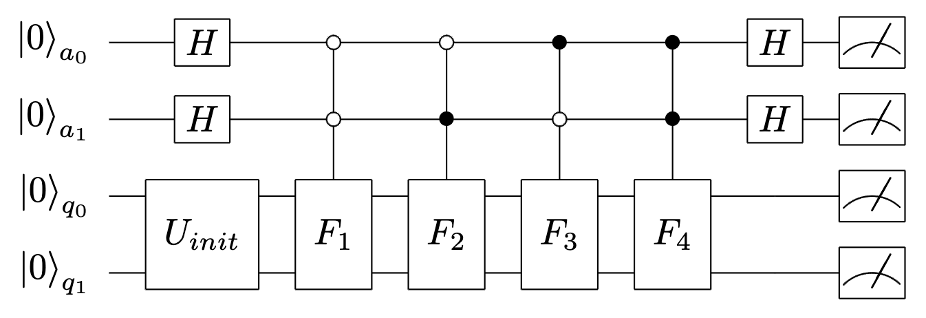
Figure 1: Quantum circuit for the Stochastic Multicloud Model (SMCM). Horizontal lines express qubits, and boxes are operations of unitary matrices for these qubits. $H$ is the hadamard gate, $U_{init}$ is an initializing unitary gate, and $F_{1},F_{2},F_{3},$ and $F_{4}$ are controlled unitary gates. The right boxes with meters mean observation. In order to obtain the cloud fraction values, calculations of this circuit must be conducted again and again.

Figure 1 is the quantum circuit we made for the SMCM. The top two qubits are ancilla qubits ($a_{0},a_{1}$), which are extra bits for the calculation. The main calculation is conducted on the bottom two qubits ($q_{0},q_{1}$). All qubits are initialized as 0. First, we create superposition states by operating the Hadamard gates on the ancilla qubits. At the same stage, we initialize the main qubits by operating $4\times 4$ unitary matrix that holds the normalized cloud fraction vector on the first column, that is,

$$U_{init}=\frac{1}{\sqrt{\sigma_{cs}^{2}+\sigma_{s}^{2}+\sigma_{d}^{2}+\sigma_{s}^{2}}}\begin{pmatrix}\sigma_{cs}&*&*&*\\ \sigma_{c}&*&*&*\\ \sigma_{d}&*&*&*\\ \sigma_{s}&*&*&*\end{pmatrix}.$$ (9)

The qubit states denoted by $\ket{\pi_{1}}$ after this operation can be written as

$$\ket{\pi_{1}}=\frac{1}{2}\left(\ket{00}_{a_{0}a_{1}}+\ket{01}_{a_{0}a_{1}}+\ket{10}_{a_{0}a_{1}}+\ket{11}_{a_{0}a_{1}}\right)\otimes\ket{\sigma}_{q_{0}q_{1}},$$ (10)

where $\otimes$ is the Kronecker product, and $\ket{\sigma}$ is the cloud fraction ket vector with four components, that is,

$$\ket{\sigma}=\frac{1}{\sqrt{\sigma_{cs}^{2}+\sigma_{s}^{2}+\sigma_{d}^{2}+\sigma_{s}^{2}}}\begin{pmatrix}\sigma_{cs}\\ \sigma_{c}\\ \sigma_{d}\\ \sigma_{s}\end{pmatrix}.$$ (11)

Next, controlled unitary gates are operated on each state as

$$\ket{\pi_{2}}=\frac{1}{2}\left(\ket{00}_{a_{0}a_{1}}\otimes F_{1}\ket{\sigma}_{q_{0}q_{1}}+\ket{01}_{a_{0}a_{1}}\otimes F_{2}\ket{\sigma}_{q_{0}q_{1}}\right.\\ \left.+\ket{10}_{a_{0}a_{1}}\otimes F_{3}\ket{\sigma}_{q_{0}q_{1}}+\ket{11}_{a_{0}a_{1}}\otimes F_{4}\ket{\sigma}_{q_{0}q_{1}}\right).$$ (12)

Finally, the Hadamard gates are operated on the ancilla qubits again to obtain the next step $\sigma$ which is encoded in the state where the ancilla qubits are $\ket{00}$. This state can be written as

$$\ket{\pi_{3}}=\frac{1}{2}\ket{00}_{a_{0}a_{1}}\otimes\left(F_{1}+F_{2}+F_{3}+F_{4}\right)\ket{\sigma}_{q_{0}q_{1}}+\ket{\lambda}_{a_{0}a_{1}q_{0}q_{1}},$$ (13)

where $\ket{\lambda}$ is a state that we are not interested in. When we observe the quantum states calculated as $\ket{\pi_{3}}$, we obtain 4-bit strings representing classical states. We derive a statistical distribution through sampling, which allows us to estimate cloud fraction states. In this approach, repeated calculations are necessary at each time step. The number of repetitions is called the shot number.

We used qiskit Aer [Qiskit contributors (2023)] simulator to compute the above algorithm. Simulation settings are similar to those described by Khouider2010. The initial fractions of $\sigma_{cs},\sigma_{c},\sigma_{d},$ and $\sigma_{s}$ were set equally at 0.25. The values of CAPE, $C=0.25$, and dryness, $D=0.75$, are used throughout the entire duration of the simulation. The integration is performed over 100 hours. Until this time, the cloud fractions reached their quasi-equilibrium states (Figure 2).

3 Results

Figure 2 displays the time evolutions of the fractions of states observed in the SMCM simulations. In the deterministic simulation, the fractions reach their equilibrium values within the first 10 hours. The equilibrium values are as follows: $\sigma_{cs}=0.46,\sigma_{c}=0.26,\sigma_{d}=0.10,$ and $\sigma_{s}=0.17$, respectively. In the case of using the classical Monte Carlo algorithm (Figure 2a), the results fluctuate around the deterministic results. These results are qualitatively similar to the results of Khouider2010. In the case of using the quantum algorithm (Figure 2b), the results are similar to that obtained with the classical Monte Carlo simulation. The transition behaviors observed in both simulations using the classical Monte Carlo and quantum algorithms closely follow the result of the deterministic simulation.

To determine the parameter that influences the fluctuation magnitudes, we conducted the same experiment with different parameter settings. Figure 3 illustrates the dependency of fluctuation magnitudes on (a) the number of lattice sites in the classical Monte Carlo simulation and (b) the shot number in the quantum algorithm. The larger the number of lattice sites in the classical Monte Carlo simulation, or the larger the number of lattice sites in the quantum simulation, the fewer the fluctuations observed. These results are consistent with the central-limit theorem. Approximately $10^{5}$ shots are required in the simulation using the quantum algorithm to achieve results similar to those obtained from the classical Monte Carlo calculation, which uses $3\times 10^{3}$ lattice sites. Why is there a difference in the number of samples required between the quantum simulation and the classical Monte Carlo simulation? The reason for the fact that the quantum algorithm needs larger sample size to obtain similar fluctuations may be explained as follows. The simulation using the quantum algorithm samples from $2^{4}$ possible states. In addition, if we rewrite the final quantum states shown in (13) as

$$\ket{\pi_{3}}=\sqrt{p_{0}}\ket{00}_{a_{0}a_{1}}\otimes\ket{\sigma}_{q_{0}q_{1}}+\sqrt{1-p_{0}}\ket{\lambda}_{a_{0}a_{1}q_{0}q_{1}}.$$ (14)

Then, the actual number of samples for the 4 states is approximately $p_{0}N$, where $p_{0}$ is the probability of obtaining the states of interest, and $N$ is the total number of shots. In our experiment, $p_{0}$ is approximately 0.25 , which significantly influences the gap in the number of samples between the classical Monte Carlo simulation and the quantum simulation. We can increase $p_{0}$ larger by using amplitude amplification; however, this method results in greater gate complexity.

4 Discussion and Conclusions

We found an atmospheric science problem to which a quantum algorithm was applicable, and actually configured a quantum circuit to compute it successfully. We implemented the algorithm on quantum circuits using Qiskit. The Qiskit transpiler decomposed these circuits into native circuits with a depth of $O(1000)$. We can roughly estimate the computation cost by multiplying this gate depth by the number of shots. It is important to note that the size of fluctuations in our algorithm is not dependent on the gate depth but is exponentially dependent on the number of shots.

Although the quantum computer cannot take full advantage of its potential in the current usage, the results of this study suggest two promising possibilities. The first is matrix calculations of transition probabilities. Probability distributions typically involve multiple dimensions, making their time development challenging to compute. Although this study tested only four states, expanding to a larger number of states could potentially reduce computational costs compared to classical computers. We expect that we could find suitable applications in the cloud droplet formation processes in weather and climate computations. The second possibility involves utilizing probabilistic outputs from computed quantum states. It may be feasible to model atmospheric phenomena where there is only one realization state that is determined according to a probability distribution.

We hope that this research will promote further studies on the usage of quantum computers in weather and climate science.

	description	value
$\tau_{01}$	decay of congestus	1 hour
$\tau_{10}$	decay of congestus	5 hours
$\tau_{12}$	conversion of congestus to deep	1 hour
$\tau_{02}$	formation of deep	2 hours
$\tau_{23}$	conversion of deep to stratiform	3 hours
$\tau_{20}$	decay of deep	5 hours
$\tau_{30}$	decay of stratiform	5 hours

Table 1: The values of $\tau_{lk}$, used in this calculation. These values correspond to case 1 of Khouider2010.

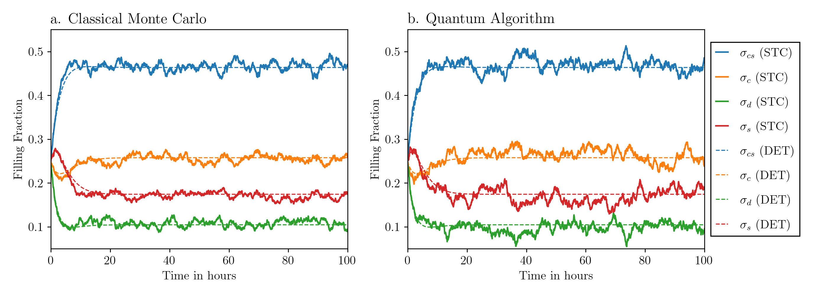
Figure 2: Time evolution of the fractions of clear sky and cloud types. In both panels, the dashed lines represent the results of the same deterministic simulation. The solid lines illustrate the results of the stochastic simulations for (a) the classical Monte Carlo algorithm, and for (b) the quantum algorithm.

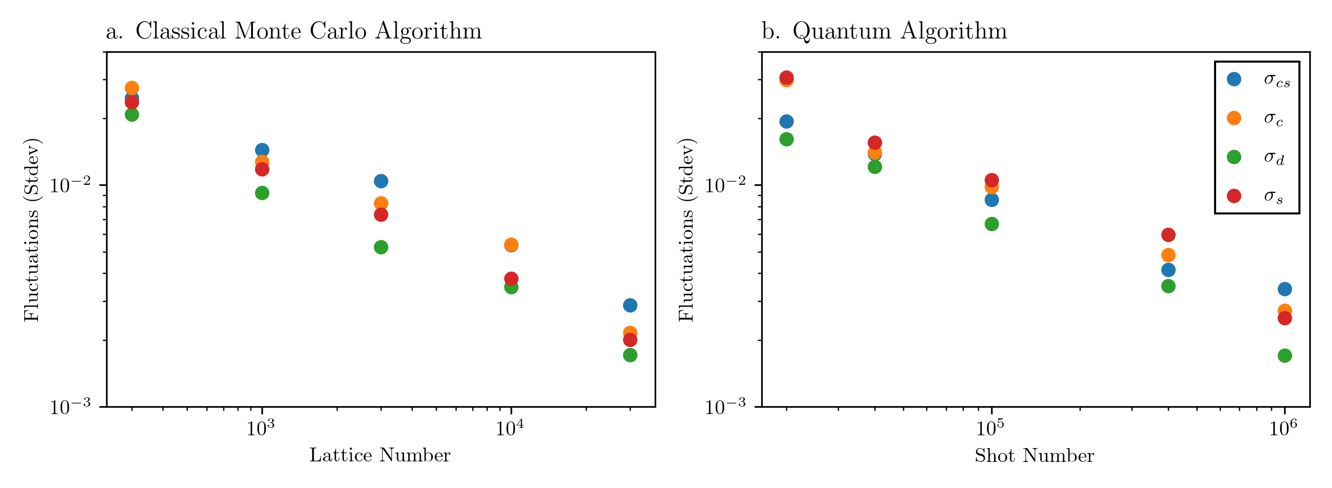
Figure 3: The degrees of fluctuations around the equilibrium states obtained by the deterministic simulation. The root-mean-squares of the stochastic values minus the deterministic value are plotted against (a) the number of lattice sites in the classical Monte Carlo algorithm, and against (b) the shot numbers in the quantum algorithm.

Open Research Section

No data sets were used or generated in this work. Code used to create and plot the results is available at GitHub (https://github.com/kazumasa-ueno/smcm_qc.git) and Zenodo (https://doi.org/10.5281/zenodo.11894586).