Full-ECE: A Metric For Token-level Calibration
on Large
Language Models
Abstract
Deep Neural Networks (DNNs) excel in various domains but face challenges in providing accurate uncertainty estimates, which are crucial for high-stakes applications. Large Language Models (LLMs) have recently emerged as powerful tools, demonstrating exceptional performance in language tasks. However, traditional calibration metrics such as Expected Calibration Error (ECE) and classwise-ECE (cw-ECE) are inadequate for LLMs due to their vast vocabularies, data complexity, and distributional focus. To address this, we propose a novel calibration concept called full calibration and introduce its corresponding metric, Full-ECE. Full-ECE evaluates the entire predicted probability distribution, offering a more accurate and robust measure of calibration for LLMs.
1 Introduction
Deep Neural Networks(DNNs) have achieved remarkable success across various domains, demonstrating superior performance in many tasks. Despite these impressive achievements, a critical challenge remains: the calibration of these models’ predictions. Calibration refers to the model’s ability to provide uncertainty estimates that accurately reflect the true likelihood of its predictions being correct. In many high-stakes applications such as healthcare Leibig et al. (2017); Dolezal et al. (2022), self-driving Michelmore et al. (2020), and protein engineering Greenman et al. (2023), it is not sufficient for a model to be highly accurate; it must also provide reliable estimates of uncertainty to ensure safety and robustness.
Large Language Models Achiam et al. (2023); Touvron et al. (2023); Brown et al. (2020) have recently emerged as powerful tools in the DNN area, demonstrating exceptional performance in a wide array of language tasks. It is essential to ensure that these models are well-calibrated at the token level. Token-level calibration refers to the alignment of the predicted probability distribution for each token with the true distribution observed in the corpus. This ensures that the probabilities assigned to each token reflect their actual occurrence likelihoods. Token-level calibration differs from traditional classification task calibration in several aspects:
-
1.
Vocabulary Size: Token-level calibration deals with a vast number of classes, typically in the hundreds of thousands according to the vocabulary size, vastly surpassing traditional classification tasks.
-
2.
Data Complexity and Imbalance: LLMs are trained on datasets containing tens of billions of tokens, introducing significant complexity and diversity compared to standard datasets. Moreover, token-level calibration grapples with highly imbalanced token distributions, posing additional challenges.
-
3.
Distribution Focus: Traditional calibration methods focus on the top-1 prediction. In contrast, token-level calibration for LLMs must account for the entire probability distribution across all tokens, as inference involves sampling from this distribution, making every token’s probability significant.
These distinctions underscore the inadequacy of traditional calibration metrics like Expected Calibration Error (ECE) Naeini et al. (2015) and classwise-ECE (cw-ECE) Kull et al. (2019) when applied to LLMs. ECE primarily considers the probability of the most likely token, which, although suitable for traditional classification tasks, fails to capture the nuances of the token distribution in LLMs. In contrast, cw-ECE evaluates calibration across each class but struggles with the extreme class imbalance and the sheer number of classes in LLMs. As the vocabulary size increases, the frequency of many tokens diminishes, making it challenging to obtain reliable calibration metrics based on these rare tokens.
To address these challenges, we propose a novel calibration concept called full calibration and introduce its corresponding metric, Full-ECE. Full-ECE evaluates the calibration of the entire predicted probability distribution, encompassing all tokens rather than focusing on the top-1 prediction. This comprehensive approach ensures that the calibration metric is robust to imbalances and vast class count of LLMs, providing a more accurate measure of LLMs’ calibration.
2 Background
Calibration refers to the process of adjusting the predictive probabilities of a model so that they reflect the true likelihood of outcomes. For example, if a model predicts an event with a probability of 70%, that event should occur approximately 70% of the time in the long run. The existing concepts of calibration can mainly be divided into two types: confidence calibration and classwise calibration.
To introduce these two types of calibration, we first need to explain some fundamental concepts. Let denote the probability distribution of data. A dataset consists of finite pairs where is a data instance and is the ground-truth class label of . A model takes in the instance and output its prediction vector . Let denote the -th dimension of .
2.1 Confidence Calibration
In confidence calibration, the index corresponding to the maximum value in the model’s predicted probability distribution is taken as the model’s prediction, and the associated probability value is considered as the model’s confidence. A model is confidence-calibrated if for any confidence ,
| (1) |
A widely used metric for evaluating confidence calibration is the ECE Naeini et al. (2015), which is defined as the expected absolute difference between the model’s confidence and its accuracy:
| (2) |
Since we only have finite samples, ECE cannot be directly calculated using the definition provided above. In practical calculations, we replace the above definition with a discretized version of ECE in which the interval is divided into equispaced bins. Let denote the indices of samples with confidences belonging to the -th bin (i.e. ). The accuracy of this bin is . The average confidence of this bin is . The discretized version of ECE is defined as
| (3) |
where is the number of samples in the dataset.
2.2 Classwise Calibration
Classwise calibration is concerned with calibrating the predicted probabilities for each individual class in a multi-class classification problem. It ensures that the predicted probabilities across different classes are accurate and properly calibrated. A model is classwise-calibrated if for any class and any probability ,
| (4) |
Similar to ECE for confidence calibration, the cw-ECE Kull et al. (2019) for classwise calibration is defined as
| (5) |
where is computed on the -th class:
| (6) |
The discretized version of cw-ECE is defined as
| (7) |
where denotes the set of indices of samples whose predicted probabilities of the -th class lie in the -th bin, and .
3 Full Calibration: Calibrating the Whole Distribution Predicted by LLMs
As mentioned earlier, ECE considers only the calibration of the most probable class in the probability distribution, while classwise-ECE (cw-ECE) takes into account the calibration of all classes in the probability distribution. However, as shown in Equations (5) and (7), for each class , cw-ECE requires calculating its corresponding ECE metric. ECE is a statistical metric that requires a sufficient number of samples for each class to be calculated accurately. In token-level calibration, it is impossible to ensure that each token appears frequently enough in the test set. We analyzed the distribution of token occurrences in a test set containing 5000 sentences and found that 30% of the tokens do not appear in the dataset at all, and 41% of the tokens appear only 1-10 times. This indicates that 71% of the tokens appear fewer than 10 times, making cw-ECE evaluation inaccurate.
To address the issues of existing calibration metrics, ECE and cw-ECE, in token-level calibration, we propose a new and more suitable calibration concept: full calibration, along with its corresponding calibration metric, Full-ECE.
Unlike confidence calibration, where the index corresponding to the maximum value in the model’s predicted probability distribution is taken as the model’s prediction, full calibration views the model’s output as a process of sampling from the predicted probability distribution. The sampled index is taken as the output token, and its corresponding probability value is considered as its confidence. A model is full-calibrated if for any , the following holds:
| (8) |
Naturally, similar to the definition of ECE, we can define the metric corresponding to full calibration as Full-ECE:
| (9) |
According to Bayes’ theorem and the law of total probability,
| (10) | ||||
Similar to the previously defined discrete ECE and cw-ECE, we divide the probability interval [0,1] of each class into equally spaced bins. Each bin represents the set of indices of samples whose predicted probabilities of the -th class lie in the -th bin. Let represent the sum of the quantities in the -th bin for all classes , i.e. . Base on (9) and (10), Full-ECE can be discretized and represented as
| Full-ECE | (11) |
where
| (12) |
and
| (13) |
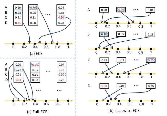
Figures 1 depicts the aggregation methods of ECE, cw-ECE, and Full-ECE for each bin. ECE focuses solely on the highest probability value within each distribution, whereas cw-ECE considers the distribution across all classes , while Full-ECE combines the statistics of different classes within the same bin. This approach addresses the issue in token-level calibration where cw-ECE faces the challenge of having too few samples for many classes.
4 The Robustness of Full-ECE
| 2B params | 7B params | |
|---|---|---|
| RSD of cw-ECE | 40.93% | 44.90% |
| RSD of Full-ECE | 7.56% | 8.36% |
Both Full-ECE and cw-ECE are metrics designed to evaluate the calibration of the entire predicted distribution. From their definitions in the discrete case, it can be observed that both of them require the probability interval [0,1] to be divided into equal-length bins. A robust metric should exhibit lower relative variation as the value of changes. We evaluated the relative standard deviation (RSD) of Full-ECE and cw-ECE for different values of in the set . Our experiments were conducted on two models: a 2-billion parameter GPT model and a 7-billion parameter GPT model trained on 1 trillion tokens. The lower the RSD, the more stable the metric is. The experimental results, shown in Table 1, demonstrate that for both models, the RSD of Full-ECE as varies is significantly lower than that of cw-ECE. Therefore, Full-ECE is more stable across different values of compared to cw-ECE, highlighting its advantage in evaluating token-level calibration in large language models.
5 Continuous Improvement of Full-ECE during LLM Training
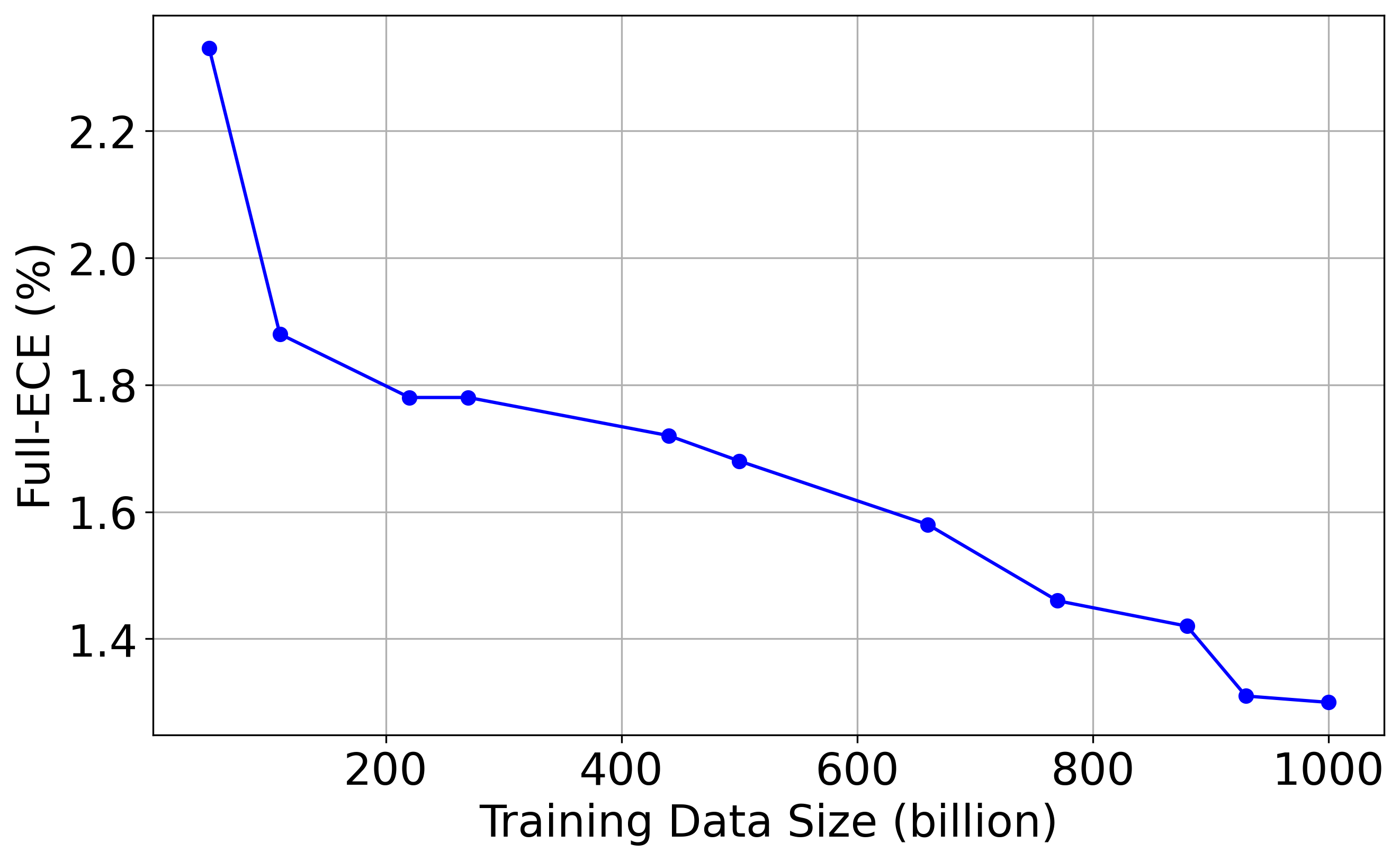
Previously, we demonstrated across different dimensions that Full-ECE is a more suitable metric than ECE and cw-ECE for evaluating uncertainty in LLMs. Another criterion for effective model evaluation is reliability and discriminability, where metrics should consistently improve with model capability. We tested the Full-ECE metric () at different training stages of the Baichuan-2 7BYang et al. (2023) model and observed a consistent downward trend (shown in Figure 2), indicating a continuous improvement in token-level calibration throughout training.
6 Conclusion
We introduce the concept of full calibration and propose its corresponding metric, Full-ECE, to address the challenges in calibrating LLMs. Unlike traditional metrics such as ECE and cw-ECE, Full-ECE evaluates the entire predicted probability distribution across all tokens, From both experimental and theoretical perspectives, we have demonstrated that Full-ECE provides a more robust calibration measure for LLMs operating with vast vocabularies and complex data distributions.
References
- Achiam et al. (2023) Josh Achiam, Steven Adler, Sandhini Agarwal, Lama Ahmad, Ilge Akkaya, Florencia Leoni Aleman, Diogo Almeida, Janko Altenschmidt, Sam Altman, Shyamal Anadkat, et al. Gpt-4 technical report. arXiv preprint arXiv:2303.08774, 2023.
- Brown et al. (2020) Tom Brown, Benjamin Mann, Nick Ryder, Melanie Subbiah, Jared D Kaplan, Prafulla Dhariwal, Arvind Neelakantan, Pranav Shyam, Girish Sastry, Amanda Askell, et al. Language models are few-shot learners. Advances in neural information processing systems, 33:1877–1901, 2020.
- Dolezal et al. (2022) James M Dolezal, Andrew Srisuwananukorn, Dmitry Karpeyev, Siddhi Ramesh, Sara Kochanny, Brittany Cody, Aaron S Mansfield, Sagar Rakshit, Radhika Bansal, Melanie C Bois, et al. Uncertainty-informed deep learning models enable high-confidence predictions for digital histopathology. Nature communications, 13(1):6572, 2022.
- Greenman et al. (2023) Kevin P Greenman, Ava P Amini, and Kevin K Yang. Benchmarking uncertainty quantification for protein engineering. bioRxiv, pp. 2023–04, 2023.
- Kull et al. (2019) Meelis Kull, Miquel Perello Nieto, Markus Kängsepp, Telmo Silva Filho, Hao Song, and Peter Flach. Beyond temperature scaling: Obtaining well-calibrated multi-class probabilities with dirichlet calibration. Advances in neural information processing systems, 32, 2019.
- Leibig et al. (2017) Christian Leibig, Vaneeda Allken, Murat Seçkin Ayhan, Philipp Berens, and Siegfried Wahl. Leveraging uncertainty information from deep neural networks for disease detection. Scientific reports, 7(1):1–14, 2017.
- Michelmore et al. (2020) Rhiannon Michelmore, Matthew Wicker, Luca Laurenti, Luca Cardelli, Yarin Gal, and Marta Kwiatkowska. Uncertainty quantification with statistical guarantees in end-to-end autonomous driving control. In International Conference on Robotics and Automation, 2020.
- Naeini et al. (2015) Mahdi Pakdaman Naeini, Gregory Cooper, and Milos Hauskrecht. Obtaining well calibrated probabilities using bayesian binning. In Proceedings of the AAAI conference on artificial intelligence, volume 29, 2015.
- Touvron et al. (2023) Hugo Touvron, Thibaut Lavril, Gautier Izacard, Xavier Martinet, Marie-Anne Lachaux, Timothée Lacroix, Baptiste Rozière, Naman Goyal, Eric Hambro, Faisal Azhar, et al. Llama: Open and efficient foundation language models. arXiv preprint arXiv:2302.13971, 2023.
- Yang et al. (2023) Aiyuan Yang, Bin Xiao, Bingning Wang, Borong Zhang, Chao Yin, Chenxu Lv, Da Pan, Dian Wang, Dong Yan, Fan Yang, Fei Deng, Feng Wang, Feng Liu, Guangwei Ai, Guosheng Dong, Haizhou Zhao, Hang Xu, Haoze Sun, Hongda Zhang, Hui Liu, Jiaming Ji, Jian Xie, Juntao Dai, Kun Fang, Lei Su, Liang Song, Lifeng Liu, Liyun Ru, Luyao Ma, Mang Wang, Mickel Liu, MingAn Lin, Nuolan Nie, Peidong Guo, Ruiyang Sun, Tao Zhang, Tianpeng Li, Tianyu Li, Wei Cheng, Weipeng Chen, Xiangrong Zeng, Xiaochuan Wang, Xiaoxi Chen, Xin Men, Xin Yu, Xuehai Pan, Yanjun Shen, Yiding Wang, Yiyu Li, Youxin Jiang, Yuchen Gao, Yupeng Zhang, Zenan Zhou, and Zhiying Wu. Baichuan 2: Open large-scale language models. arXiv preprint arXiv:2309.10305, 2023. URL https://arxiv.org/pdf/2309.10305.