LFPLM: A General and Flexible Load Forecasting Framework based on Pre-trained Language Model

Abstract

Accurate load forecasting is essential for maintaining the power balance between generators and consumers, especially with the increasing integration of renewable energy sources, which introduce significant intermittent volatility. With the development of data-driven methods, machine learning and deep learning-based models have become the predominant approach for load forecasting tasks. In recent years, pre-trained language models (PLMs) have made significant advancements, demonstrating superior performance in various fields. This paper proposes a load forecasting method based on PLMs, which offers not only accurate predictive ability but also general and flexible applicability. Additionally, a data modeling method is proposed to effectively transform load sequence data into natural language for PLM training. Furthermore, we introduce a data enhancement strategy that eliminate the impact of PLM hallucinations on forecasting results. The effectiveness of the proposed method has been validated on two real-world datasets. Compared with existing methods, our approach shows state-of-the-art performance across all validation metrics.

I Introduction

Load forecasting has been playing an important role in maintaining the stability of the modern power system[1]. With accurate forecasting results, the power system can maximize the integration of unstable renewable energy sources such as photovoltaic and wind power[2]. In recent years, machine learning and deep learning-based methods have become the mainstream approach for load forecasting tasks due to their outstanding performance[3, 4, 5]. Various networks have been continuously adapted to promote the prediction accuracy, such as eXtreme Gradient Boosting (XGBoost)[6], Random Forest (RF)[7] and Long Short-Term Memory (LSTM)[8].

Beyond the model itself, the quality and distribution of data used for training above models also make a difference to the forecasting accuracy. To ensure the model performs optimally on general task, data modeling and feature engineering strategies designed for specific model are often proposed at the same time. Reference [9] adapts a XGBoost-based scheme for electricity load forecasting through increasing number of features available and converting daily electricity load information into weekly load information. Reference [10] demonstrates the flexibility of RF-based load forecasting associated with expert selection to fit with complex customers behavior. In [11], a residential load forecasting framework based on the LSTM is described with an customer-wise level data analysis. Facing the growing diversity of load data from different scenario, the limited ability of a single model sometimes hardly achieve high-precision predictions. Some research combines several methods together to improve the general performance consequently. The RF and Mean Generating Function is mixed with an adjustable weight parameter for short-term load forecasting[12]. Reference[13] proposes a hybrid methodology to forecast short-term electrical load based on the integration of Convolutional Neural Network(CNN) and LSTM network. Reference [14] illustrates a load forecasting model based on the Temporal Convolutional Network(TCN) and Light-GBM, extending the application to multiple different types of industrial customers.

More recently, pre-trained language models (PLMs) have emerged, demonstrating strong accuracy and flexibility across various research in deep learning field[15, 16]. The Attention mechanism in PLMs models have been proven to be effective in capturing the long-range dependencies in time series data, which is beneficial for load forecasting tasks[17, 18]. Some ongoing research are already applying PLMs to predict time series sequences. Reference [19] introduces a prompt-based learning paradigm for time series forecasting, where user’s own dataset is directly trained on the models. Reference [20] tokenizes the prompts and completes the training by updating the reprogramming layer parameters, while keeping the parameters of large language model static. However, PLMs also have their own limitations that the hallucination is generally inevitable across various downstreams research[21, 22]. In load forecasting tasks, the hallucination may lead to extremely inaccurate predictions or missing values in the output sequence. In [19], the missing rate metric is proposed to evaluate the hallucination, but there is few research on how to effectively solve the hallucination problem in load forecasting tasks.

Hence, this paper proposes a load forecasting framework called LFPLM, leveraging its flexibility and generalizability to achieve more accurate results on multi-time-scale and multi-scenario datasets. Also, the paper introduces a dataset modeling method that enables PLMs to perform effectively. To the best of the authors’ knowledge, our work is the first research that applying PLMs on load forecasting tasks in power system.

The specific contributions of this research are as follows:

1. Propose a general and flexible load forecasting method in power system based on PLMs. The proposed method can be applied to various load forecasting tasks with different time scales.

2. Propose a dataset formulation method that combine language with statistical information to better leverage the predictive capabilities of PLMs.

3. Propose a data enhancement method for solving the the hallucination problems of PLMs by separating numerical sequence with language descriptions.

4. Validate the effectiveness of the proposed method across open-sources and real-world load forecasting datasets with different time scales. Compared with existing load forecasting methods, the superiority and adaptability of the proposed framework is clearly proved.

TABLE I: The example of Dataset based on proposed method

Input Data	$\boldsymbol{L\times d}$	Example	Ground-truth
$X_{text}$	ELFD: 7$\times$1 ICLD: 24$\times$1	The electricity consumption of each day is as follows, 29979,29415,27958,25579,28112,29664,29516kWh. What is the daily consumption of next week?	The electricity consumption of each day is as follows, 22992,21895,26303,28286,28727,26488,24839kWh.
$X_{ts}$	ELFD: 7$\times$1 ICLD: 24$\times$1	The electricity consumption of each day is as follows, 29979,29415,27958,25579,28112,29664, 29516kWh. The maximum value is 32123, the minimun value is 20321, the average value is 28603. What is the daily consumption of next week?	The electricity consumption of each day is as follows, 22992,21895,26303,28286,28727,26488,24839kWh.
$X_{ets}$	ELFD: 7$\times$1 ICLD: 24$\times$1	The electricity consumption of each day is as follows, day one: 29979, day two: 29415, day three: 27958, day four: 25579, day five:28112, day six: 29664, day seven: 29516kWh. The maximum value is 32123, the minimun value is 20321, the average value is 28603. What is the daily consumption of next week?	The electricity consumption of each day is as follows, day one: 22992, day two: 21895, day three: 26303, day four: 28286, day five:28727, day six:26488, day seven: 24839kWh.

• For datasets in other languages, we use Google Translate to generate corresponding input data and Ground-truth in the identical format.

II Dataset Description and Formulation

In this section, we present a method for creating datasets to train LFPLM. Starting with converting numerical data into textual data, we will detail our approaches through which we can effectively fine-tuning the model. Moreover, a technique to address the hallucination phenomenon of PLMs is also introduced. To emphasize, the proposed dataset modeling method is applicable to all load forecasting tasks based on PLMs.

II-A Combine Language with Statistical Information

In common load forecasting tasks, historical load data are always employed as the input for forecasting. The input data are typically modelled into a continuous sequence $X\in\mathbb{R}^{L\times d}$, where $L$ and $d$ represents the length and dimension of the sequence, respectively. Since data is required to be input in text format for LFPLM, we propose a dataset modeling method that convert numerical sequence into natural language expression $X_{text}$ as described below:

$$X_{text}=\{\mathbb{S}(x_{1})\ ...\ \mathbb{S}(x_{i})\}\qquad for\ 1\leq i\leq L\hfill$$ (1)

where $x_{i}$ is the $i$-th data in the input sequence, $\mathbb{R}$ represents the set of real number, $\mathbb{S}$ stands for the transformation from real number to text.

Additionally, to further exploit the advantages of textual expression, we introduce statistical information $X_{stat}$ to enhance the feature dimension of the input data, denoted as $X_{ts}$. The statistical information includes the maximum, minimum, and average values. Specifically, we use the maximum and minimum values within the range of $N_{obs}$ steps before the predicted time to model global features, and represent the local features with the average value of the input sequence.

$$\left\{\begin{array}[]{l}X_{ts}=\{X_{text},X_{stat}\}\hfill\hfill\\ X_{stat}=\{Max(X_{obs}),Min(X_{obs}),\\ \qquad\qquad\qquad Average(X)...\}\hfill\hfill\end{array}\right.$$ (2)

where $X_{ts}$ represents the input with statistical information of PLM, $X_{stat}$ is the statistical information with language descriptions including the maximum, minimum and average value of $X$, $X_{obs}$ demonstrate the historical load data within the range of $N_{obs}$ time-steps before the predicted time.

II-B Separate Numerical Sequence with Language

The causes of hallucination in load forecasting tasks, such as missing data or generating extra data, can be attributed to two primary aspects: 1) during the conversion of numerical data to textual descriptions, the lengths of loaded data stored in string format exhibit inconsistency. 2) the pre-training parameters of PLMs are derived from training on natural language, thereby lacking the capability to effectively recognize purely numerical values.

Taking advantages of PLM’s sensitivity to language descriptions, this section proposes a data enhancement method that separates numerical data with textual information. The enhanced input dataset $X_{ets}$ is constructed based on $X^{*}_{text}$ as shown below:

$$\left\{\begin{array}[]{l}X_{ets}=\{X^{*}_{text},X_{stat}\}\hfill\hfill\\ X^{*}_{text}=\{(t_{1},x_{1})\ ...\ (t_{i},x_{i})\}\qquad for\ 1\leq i\leq L\hfill\\ X_{stat}=\{Max(X_{obs}),Min(X_{obs}),\\ \qquad\qquad\qquad Average(X)...\}\hfill\hfill\end{array}\right.$$ (3)

where $X^{*}_{text}$ is the textual expression of the numerical sequence with time information, $t_{i}$ is the $i$-th corresponding time-steps in textual expression of $x_{i}$.

Given that the output data from LFPLM also exists in text form, the textual ground-truth is necessary for the training process consequently. Following the same process for each input format of $X$, we generate the corresponding ground-truth $Y_{gt}$.

II-C Dataset for Forecasting

To evaluate the generality and accuracy of the proposed methods in load forecasting tasks, we selected the following two real-world datasets at different time scales to perform our research.

II-C1 Electricity Load Forecasting Dataset (ELFD)

This is an open-source dataset available on Kaggle, covering over 40,000 hourly load data for the Panama region from 2015 to 2020. The dataset can be accessed via the following URL on kaggle.com/datasets/saurabhshahane/electricity-load-forecasting/data.

II-C2 Industrial Clients Load Dataset (ICLD)

This real-world dataset comprises around 9000 daily load data on the electricity consumption of the 10 industrial clients from 2018 to 2021. The dataset is collected from a real-world power system in east China.

The distribution of two dataset is visualized in Figure 1. Dataset with detailed examples under the strategies established in this section is shown in Table I. The effectiveness of proposed methods above are validated in Section IV.

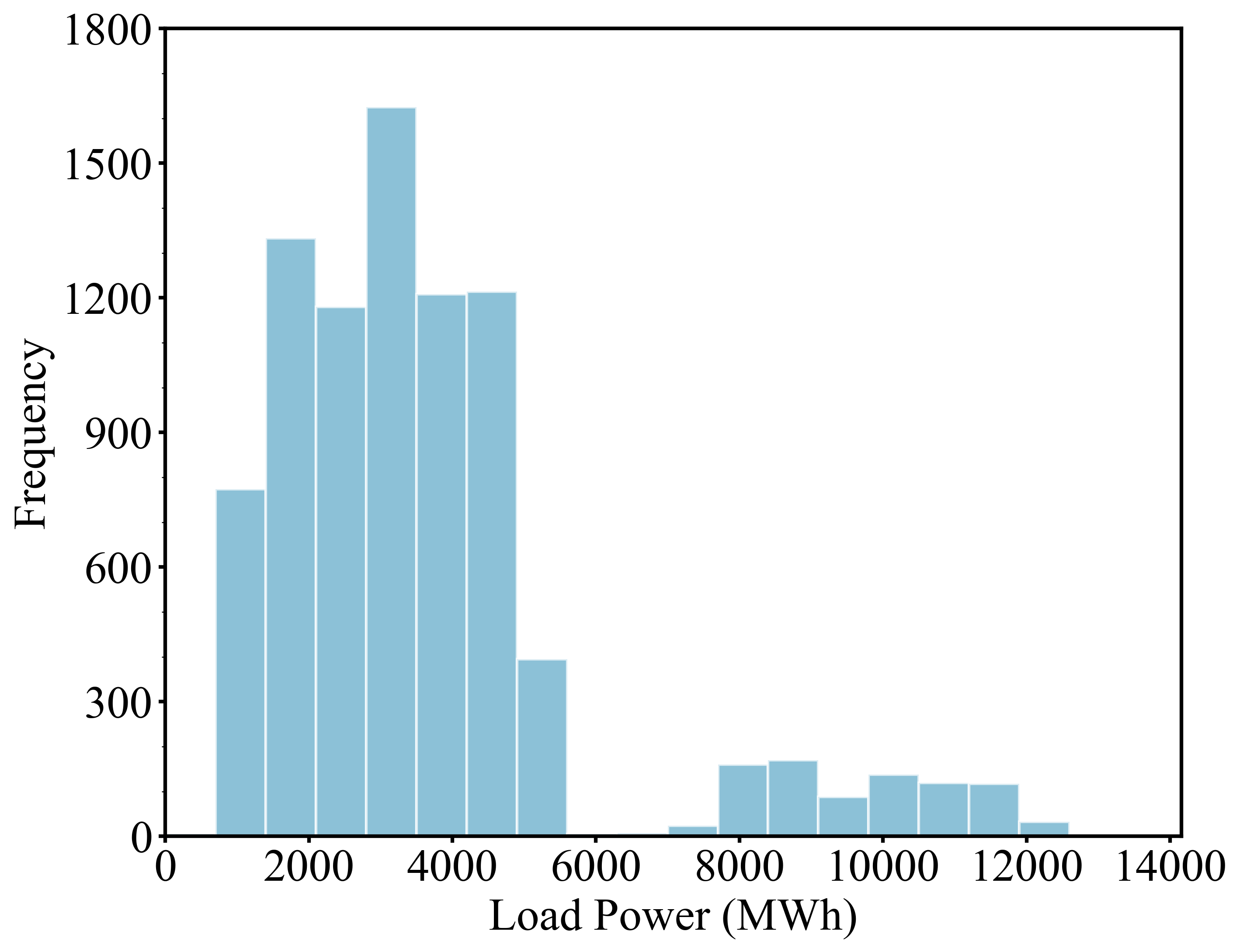
(a) ICLD

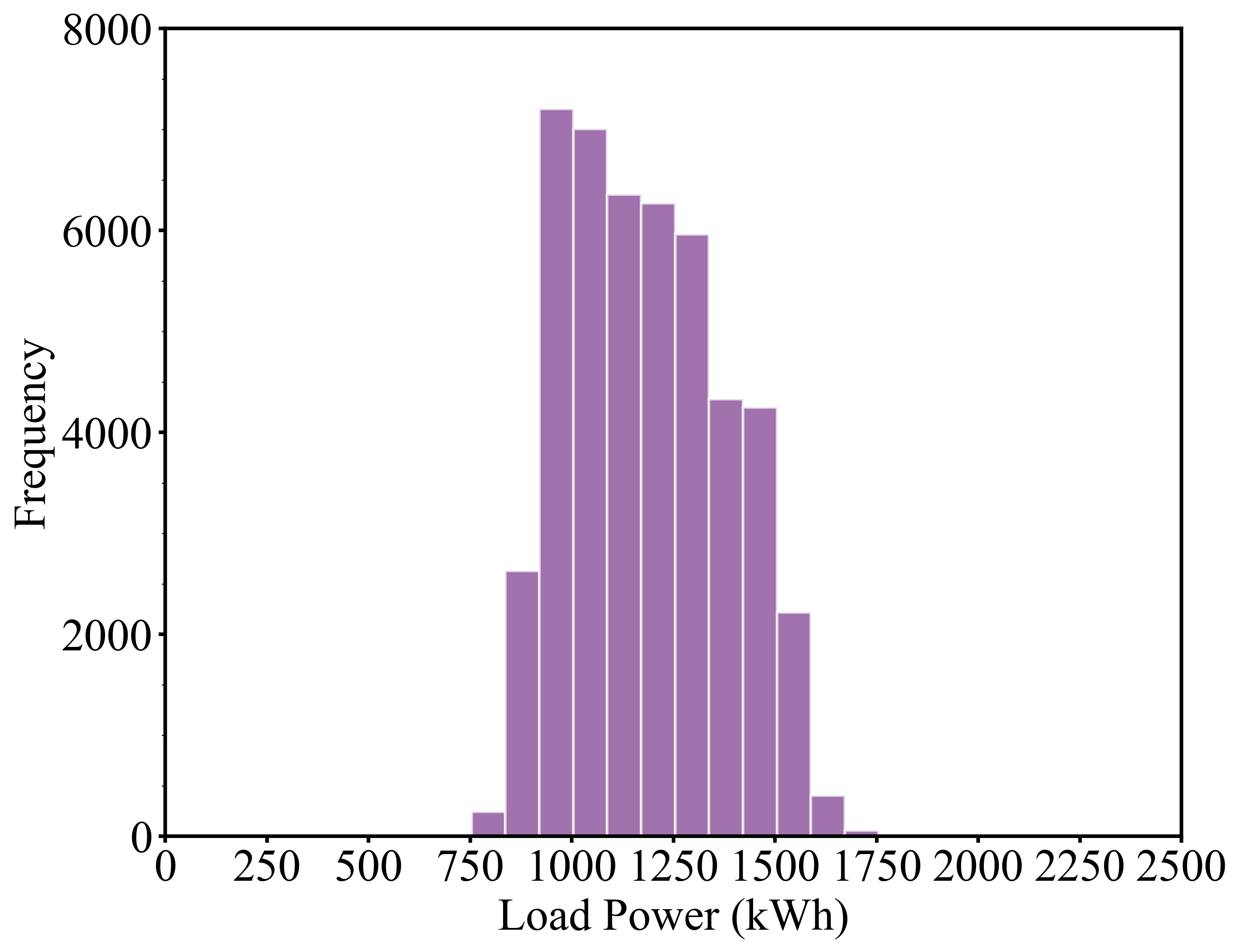
(b) ELFD

Figure 1: Distribution of involved load forecasting datasets

III Proposed Framework

In this section, we provide a detailed introduction to the basic structure of our proposed prediction framework and the PLMs used to complete the prediction task. Additionally, we detail training methods for different PLMs and list the metrics used to evaluate their forecasting results.

III-A PLMs for Load Forecasting

PLMs could be structurally categorized into three types:

TABLE II: The PLM Models used in the Proposed Framework

Model	Pre-trained Language	Access Key	Model Size
BART BART-CN	English Chinese	facebook/bart-base fnlp/bart-base-chinese	558MB 561MB
T5 Mengzi-T5	English Chinese	google-t5/t5-base Langboat/mengzi-t5-base	892MB 990MB
BigBird	English	google/bigbird-pegasus- large-arxiv	2.3GB
BLOOM BLOOM-CN	English Chinese	bigscience/bloom-1b7 Langboat/bloom-1b4-zh	3.4GB 5.6GB

Encoder-Only Models: Represented by BERT[23], these models learn bidirectional context encoders through masked language modeling. The training objective involves randomly masking parts of the text and predicting the masked words. This architecture is mainly suitable for tasks that do not require sequence generation but instead need to encode and process input, such as text classification and sentiment analysis.

Decoder-Only Models: Represented by GPT[24] and BLOOM[25], these models are typically used for sequence generation tasks and known as generative model. It generates sequences directly from the input and perform unsupervised pre-training. However, they require tremendous training data to improve the quality and diversity of generated text.

Encoder-Decoder Models: Represented by T5[26] and BART[27], these models use an encoder to process the input sequence, extracting features and semantic information, and a decoder to generate the corresponding output sequence. Known as sequence-to-sequence model, it experts in handling the relationship between input and output sequences, improving accuracy in tasks like machine translation and dialogue generation.

Depending on the characteristics of load forecasting tasks, we primarily considers PLMs based on Decoder-only and Encoder-Decoder architectures as shown in Table II. Furthermore, PLMs trained in different languages are selected to verify whether the forecasting result is influenced by natural language expression.

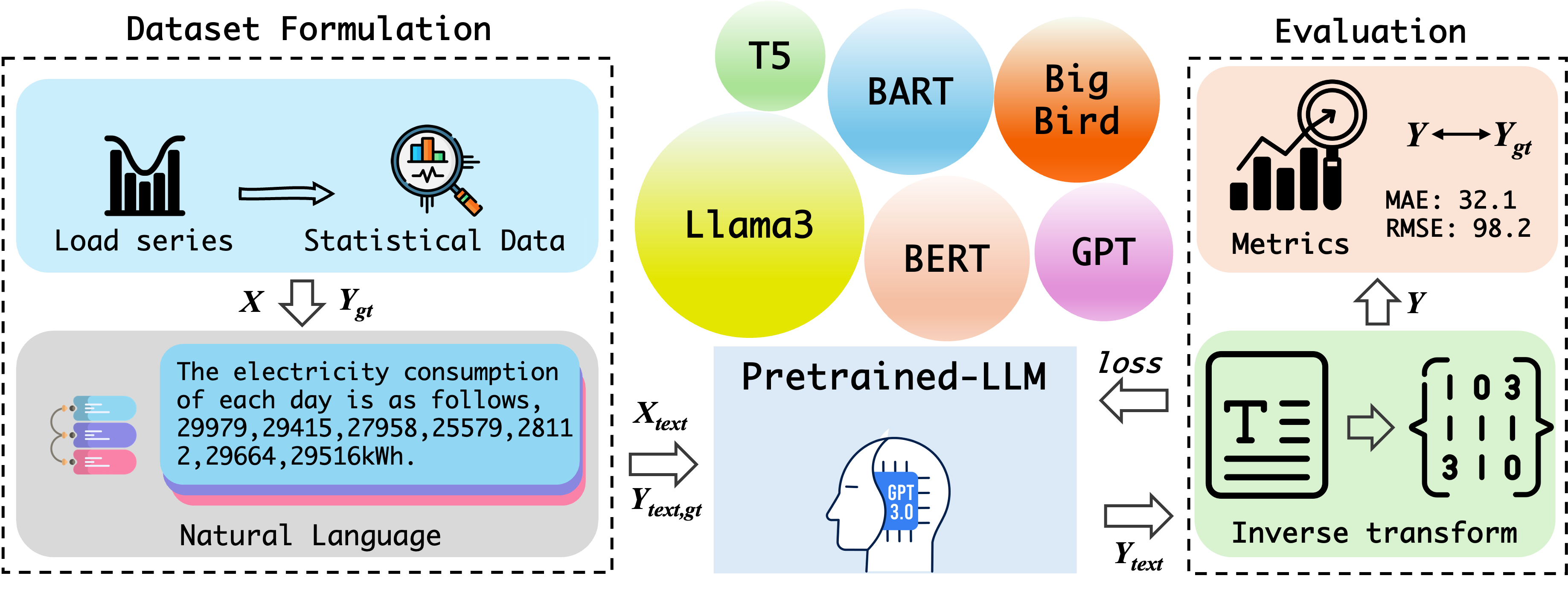
Figure 2: The architecture of the proposed LFPLM framework.

III-B Training Strategies for Different PLMs

The framework of our work is depicted in Figure 2. To fully leverage the pre-trained parameters in large models, we adopt diverse training approaches for various PLMs, aiming to achieve optimal prediction results while maintaining training efficiency.

III-B1 Full Parameter Training

A fully parameterized training method under LFPLM is served to train PLMs (except for BLOOM) with the proposed dataset. Although this approach sacrifices original problem-solving capability for their own pre-trained parameters, it can perform well in load forecasting tasks.

III-B2 Parameter-Efficient Fine-Tuning (PEFT)

Large language models such as BLOOM, pre-trained for general tasks, encode a comprehensive understanding of knowledge within their pre-trained parameters. However, training these models completely on specialized datasets will destroy the distribution pattern of pre-trained parameters, reducing their feasibility in text comprehension. Therefore, we adoption PEFT method with the Low-Rank Adaptation of Large Language Models (LoRA) technique to delicately fine-tune model parameters[28]. In this method, we use low-rank decomposition to simulate parameter changes based on the original model’s parameter distribution, thereby indirectly training a large model with a minimal number of parameters. We process the selected parameter matrix $W_{d\times k}$ from the original model as follows:

$$W_{d\times k}=U_{d\times r}\cdot V_{r\times k}\qquad r\ll d,k$$ (4)

where $r$ is the Low-rank coefficient, $U$ and $V$ are the low-rank matrices.

In our research, the parameters selected for PEFT is the $W_{Q}$, $W_{K}$ and $W_{V}$ metrics in the self-attention layers and the total amount of trainable parameters takes up to 10% of the original model.

III-C Evaluation Method and Metrics

For the model’s prediction results, we mostly care about the accuracy of the numerical sequence within natural language. According to the format setting of ground-truth in Section II, we can easily extract the data sequence from the text, with which we can calculate the forecasting accuracy to analyse the performance of the model.

Hallucination Rate is proposed to evaluate the hallucination in the forecasting results. Together with the Mean Absolute Error (MAE) and Root Mean Square Error (RMSE), three metrics are served as evaluation metrics in our research and defined as follows,

$$H=\frac{n_{h}}{N}$$ (5)

$$MAE=\frac{1}{N}\sum_{i=1}^{N}\left|Y_{i}-Y_{i,gt}\right|$$ (6)

$$RMSE=\sqrt[]{\frac{1}{N}\sum_{i=1}^{N}\left(Y_{i}-Y_{i,gt}\right)^{2}}$$ (7)

where $N$ is the number of samples, $Y_{i}$ is the $i$-th predicted result, $Y_{i,gt}$ is the corresponding ground-truth, $H\in(0,1)$ is the Hallucination Rate and $n_{h}$ is the number of hallucination samples.

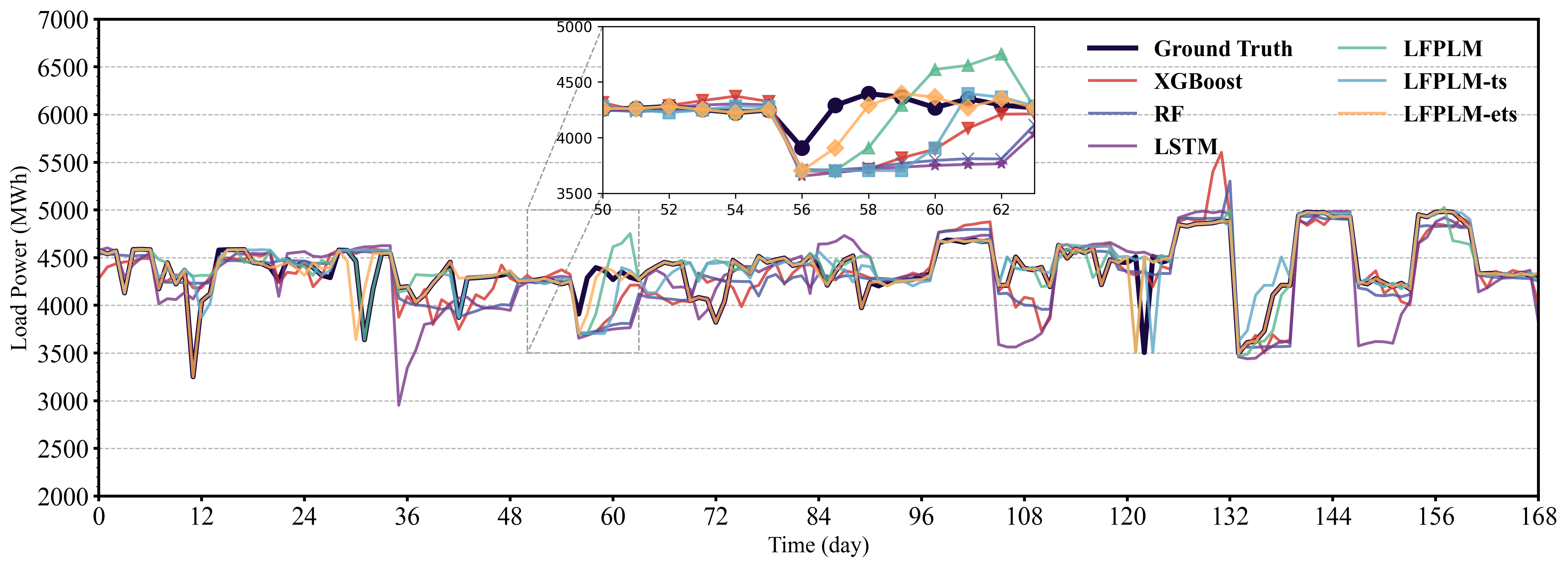
Figure 3: Forecasting results comparison of the proposed method with other models on ICLD.

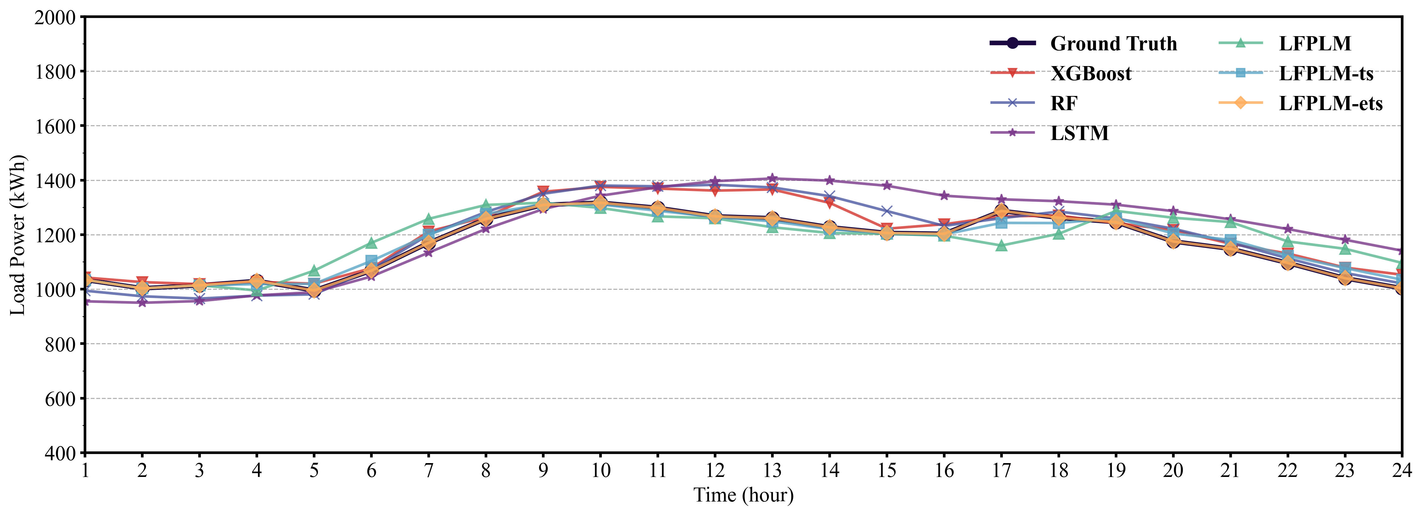
Figure 4: Forecasting results comparison of the proposed method with other models on ELFD.

IV Case study

In this section, we will validate the effectiveness of the proposed methods. Firstly, we will demonstrate the physical environment and hyperparameter configurations employed during training. Secondly, we will apply the LFPLM forecasting framework to two datasets introduced in Section II. Mengzi-T5 model as a representation of PLMs, will undergo an in-depth evaluation of its performance and statistical outcomes compared with traditional methods. Furthermore, the various PLMs mentioned in Section III will be tested to confirm their capabilities in the prediction task.

IV-A Parameters Configuration

Our model is implemented using PyTorch and Transformers from HuggingFace, with all experiments conducted on NVIDIA 4090-24G GPUs. All of our models can be accessed with the Access Key in Table II from HuggingFace Model Hub[29]. The hyperparameters of the proposed framework and comparison methods are shown in Table IV.

TABLE III: Comparison between Different Methods and LFPLM

Method	Input Data	ICLD			ELFD
		Hallucination Rate	MAE	RMSE	Hallucination Rate	MAE	RMSE
XGBoost	$X$	0	130.5	219.5	0	73.5	97.3
Random Forest	$X$	0	122.4	199.5	0	65.5	90.2
LSTM	$X$	0	172.4	294.6	0	67.15	94.37
LFPLM	$X_{text}$	0.035	264.5	2987.1	0.085	6.8	230.6
LFPLM-ts	$X_{ts}$	0.022	79.8	182.4	0.016	5.9	29.8
LFPLM-ets	$X_{ets}$	0	40.6	137.8	0	4.0	17.8

TABLE IV: Hyperparameters of LFPLM and Comparison Methods

Method	Hyperparameters	Value
LFPLM	Per device train batch size Per device eval batch size Gradient accumulation steps Learning rate Metric for best model Early stopping patience Input length of ICLD Output length of ICLD Input length of ELFD Output length of ELFD Random seed LoRA coefficient LoRA alpha LoRA dropout LoRA target modules	16 32 2 $5e^{-5}$ eval_loss 5 7 7 24 24 42 8 8 0 $query\_key\_values$
XGBoost	Number of estimators Learning rate Max depth	160 0.01 10
Random Forest	Number of estimators Max depth	160 10
LSTM	Number of layers Hidden size Dropout rate Batch size Learning rate	10 128 0.2 32 0.001

IV-B Forecasting Results of Different Time-scale Datasets

In the validation sets of ICLD and ELFD, with lengths of 860 and 2670 respectively, we calculate the Hallucination Rate, MAE and RMSE of the predicted data. The hallucination of PLMs may result in missing or excess issues with the results. To ensure the calculation of metrics, we address this problem as follows: 1)missing data is handled by supplementing it with zeros, 2)additional data is removed to keep the same length of all output sequences. We employ Mengzi-T5 model for our LFPLM framework and compare it with traditional methods including XGBoost, Random Forest, and LSTM. As depicted in Table III, the LFPLM method shows state-of-the-art performance compared to three traditional prediction methods. The LFPLM, LFPLM-ts, and LFPLM-ets methods are only different in the input data format corresponding to $X_{text}$, $X_{ts}$, and $X_{ets}$. The prediction results suggest that integrating long-vision statistical information into the data enhances prediction accuracy. To provide a intuitional presentation, forecasting curves of the LFPLM compared with other methods are visualized in Figures 3 and Figure 4.

Notably, the red data in Table III highlights the impact of the hallucination problem within forecasts, particularly in the ICLD dataset, where it results in a significantly higher RMSE than normal values. We confirm that this issue arises from a missing value in the predicted data sequence. With $X_{ets}$ as the input data, the hallucination rate is reduced to zero, and the MAE and RMSE are also significantly improved.

These result demonstrates that without preprocessing the original data, the predictive capability of PLM is under-explored. With the proposed method in Section II, LFPLM can effectively eliminate hallucination and improve the forecasting accuracy.

IV-C Forecasting Results based on Different PLMs Models

We validated the generality of our approach on PLMs with different structures given in Table II. As shown in Table V, the LFPLM-based prediction framework consistently achieves low MAE and RMSE across different PLMs, and the Mengzi-T5 model shows the best prediction performance on both datasets. The results also indicate that models based on pre-training parameters in Chinese and corresponding dataset perform better in prediction tasks. We achieved better forecasting results with two Chinese pre-trained models: Mengzi-T5 and BART-CN.

The BLOOM and BLOOM-CN models, using our proposed data modeling method combined with PEFT, do not perform well in load forecasting tasks. The output of models is inaccurate with a large number of hallucinations, such as The electricity consumption is 1834,133,12699,,- - -,192,, Although the textual part of their outputs can reflect some training information, the numerical outputs exhibit significant distortions. Therefore, the results of these two models are excluded from the statistics.

TABLE V: Comparison between Different PLM backbones

Model	ICLD		ELFD
	MAE	RMSE	MAE	RMSE
T5	135.2	242.9	27.9	75.1
Mengzi-T5	40.6	137.8	4.0	17.8
BART	97.5	216.3	25.5	60.2
BART-CN	60.0	167.5	4.8	23.8
BigBird	99.5	207.6	30.8	73.6
BLOOM	-	-	-	-
BLOOM-CN	-	-	-	-

V Conclusion

In this paper, a general and flexible load forecasting framework based on pre-trained language models is proposed. The following conclusions can be drawn:

1. A dataset formulation approach is established to convert sequence-formatted data into natural language to facilitate PLM training and language descriptions of statistical information is integrated for broaden the input feature dimension.

2. A data enhancement method is accordingly proposed to address the hallucination problem of PLMs in load prediction tasks. With the proper separation of numerical sequence and language descriptions, the hallucination rate is significantly reduced to 0%.

3. The comprehensive predictive performance of LFPLM is validated on two real-world datasets. The MAE of LFPLM is reduced to 40.6 and 4.0 on ICLD and ELFD respectively, demonstrating superior prediction accuracy over existing methods.

In future work, we aim to apply larger language models on load prediction problems. We will focus on establishing datasets and developing training methods suitable for large language models, ensuring reliable load prediction while maximizing the utilization of pre-trained parameters. Besides, the reason why Chinese pre-trained models perform better in load forecasting tasks is still unclear, and we will keep investigating the underlying reasons. Furthermore,we will also explore the potential of PLMs in other power system tasks, such as fault diagnosis and power quality analysis.

References

- [1] P. Kundur, “Power system stability,” Power system stability and control, vol. 10, pp. 7–1, 2007.
- [2] A. S. Brouwer, M. Van Den Broek, A. Seebregts, and A. Faaij, “Impacts of large-scale intermittent renewable energy sources on electricity systems, and how these can be modeled,” Renewable and Sustainable Energy Reviews, vol. 33, pp. 443–466, 2014.
- [3] A. K. Singh, S. Khatoon, M. Muazzam, D. K. Chaturvedi et al., “Load forecasting techniques and methodologies: A review,” in 2012 2nd International Conference on Power, Control and Embedded Systems. IEEE, 2012, pp. 1–10.
- [4] A. Almalaq and G. Edwards, “A review of deep learning methods applied on load forecasting,” in 2017 16th IEEE international conference on machine learning and applications (ICMLA). IEEE, 2017, pp. 511–516.
- [5] S. Fan, L. Chen, and W.-J. Lee, “Machine learning based switching model for electricity load forecasting,” Energy Conversion and Management, vol. 49, no. 6, pp. 1331–1344, 2008.
- [6] T. Chen and C. Guestrin, “Xgboost: A scalable tree boosting system,” in Proceedings of the 22nd acm sigkdd international conference on knowledge discovery and data mining, 2016, pp. 785–794.
- [7] L. Breiman, “Random forests,” Machine learning, vol. 45, pp. 5–32, 2001.
- [8] S. Hochreiter and J. Schmidhuber, “Long short-term memory,” Neural computation, vol. 9, no. 8, pp. 1735–1780, 1997.
- [9] R. A. Abbasi, N. Javaid, M. N. J. Ghuman, Z. A. Khan, S. Ur Rehman, and Amanullah, “Short term load forecasting using xgboost,” in Web, Artificial Intelligence and Network Applications: Proceedings of the Workshops of the 33rd International Conference on Advanced Information Networking and Applications (WAINA-2019) 33. Springer, 2019, pp. 1120–1131.
- [10] A. Lahouar and J. Ben Hadj Slama, “Day-ahead load forecast using random forest and expert input selection,” Energy Conversion and Management, vol. 103, pp. 1040–1051, 2015. [Online]. Available: https://www.sciencedirect.com/science/article/pii/S0196890415006925
- [11] W. Kong, Z. Y. Dong, Y. Jia, D. J. Hill, Y. Xu, and Y. Zhang, “Short-term residential load forecasting based on lstm recurrent neural network,” IEEE transactions on smart grid, vol. 10, no. 1, pp. 841–851, 2017.
- [12] G.-F. Fan, L.-Z. Zhang, M. Yu, W.-C. Hong, and S.-Q. Dong, “Applications of random forest in multivariable response surface for short-term load forecasting,” International Journal of Electrical Power & Energy Systems, vol. 139, p. 108073, 2022.
- [13] S. H. Rafi, S. R. Deeba, E. Hossain et al., “A short-term load forecasting method using integrated cnn and lstm network,” IEEE access, vol. 9, pp. 32 436–32 448, 2021.
- [14] Y. Wang, J. Chen, X. Chen, X. Zeng, Y. Kong, S. Sun, Y. Guo, and Y. Liu, “Short-term load forecasting for industrial customers based on tcn-lightgbm,” IEEE Transactions on Power Systems, vol. 36, no. 3, pp. 1984–1997, 2021.
- [15] H. Wang, J. Li, H. Wu, E. Hovy, and Y. Sun, “Pre-trained language models and their applications,” Engineering, 2022.
- [16] B. Min, H. Ross, E. Sulem, A. P. B. Veyseh, T. H. Nguyen, O. Sainz, E. Agirre, I. Heintz, and D. Roth, “Recent advances in natural language processing via large pre-trained language models: A survey,” ACM Computing Surveys, vol. 56, no. 2, pp. 1–40, 2023.
- [17] H. Zhou, S. Zhang, J. Peng, S. Zhang, J. Li, H. Xiong, and W. Zhang, “Informer: Beyond efficient transformer for long sequence time-series forecasting,” in Proceedings of the AAAI conference on artificial intelligence, vol. 35, no. 12, 2021, pp. 11 106–11 115.
- [18] Y. Qin, D. Song, H. Chen, W. Cheng, G. Jiang, and G. Cottrell, “A dual-stage attention-based recurrent neural network for time series prediction,” arXiv preprint arXiv:1704.02971, 2017.
- [19] H. Xue and F. D. Salim, “Promptcast: A new prompt-based learning paradigm for time series forecasting,” IEEE Transactions on Knowledge and Data Engineering, 2023.
- [20] M. Jin, S. Wang, L. Ma, Z. Chu, J. Y. Zhang, X. Shi, P.-Y. Chen, Y. Liang, Y.-F. Li, S. Pan et al., “Time-llm: Time series forecasting by reprogramming large language models,” arXiv preprint arXiv:2310.01728, 2023.
- [21] Z. Xu, S. Jain, and M. Kankanhalli, “Hallucination is inevitable: An innate limitation of large language models,” arXiv preprint arXiv:2401.11817, 2024.
- [22] H. Ye, T. Liu, A. Zhang, W. Hua, and W. Jia, “Cognitive mirage: A review of hallucinations in large language models,” arXiv preprint arXiv:2309.06794, 2023.
- [23] J. Devlin, M. Chang, K. Lee, and K. Toutanova, “BERT: pre-training of deep bidirectional transformers for language understanding,” CoRR, vol. abs/1810.04805, 2018. [Online]. Available: http://arxiv.org/abs/1810.04805
- [24] A. Radford, J. Wu, R. Child, D. Luan, D. Amodei, and I. Sutskever, “Language models are unsupervised multitask learners,” 2019.
- [25] T. Le Scao, A. Fan, C. Akiki, E. Pavlick, S. Ilić, D. Hesslow, R. Castagné, A. S. Luccioni, F. Yvon, M. Gallé et al., “Bloom: A 176b-parameter open-access multilingual language model,” 2023.
- [26] Z. Zhang, H. Zhang, K. Chen, Y. Guo, J. Hua, Y. Wang, and M. Zhou, “Mengzi: Towards lightweight yet ingenious pre-trained models for chinese,” 2021.
- [27] M. Lewis, Y. Liu, N. Goyal, M. Ghazvininejad, A. Mohamed, O. Levy, V. Stoyanov, and L. Zettlemoyer, “BART: denoising sequence-to-sequence pre-training for natural language generation, translation, and comprehension,” CoRR, vol. abs/1910.13461, 2019. [Online]. Available: http://arxiv.org/abs/1910.13461
- [28] N. Ding, Y. Qin, G. Yang, F. Wei, Z. Yang, Y. Su, S. Hu, Y. Chen, C.-M. Chan, W. Chen et al., “Parameter-efficient fine-tuning of large-scale pre-trained language models,” Nature Machine Intelligence, vol. 5, no. 3, pp. 220–235, 2023.
- [29] T. Wolf, L. Debut, V. Sanh, J. Chaumond, C. Delangue, A. Moi, P. Cistac, T. Rault, R. Louf, M. Funtowicz, and J. Brew, “Huggingface’s transformers: State-of-the-art natural language processing,” CoRR, vol. abs/1910.03771, 2019. [Online]. Available: http://arxiv.org/abs/1910.03771