Joint Distributed Generation Maximization and Radial Distribution Network Reconfiguration

Abstract

This paper studies an optimization problem for joint radial distribution system network reconfiguration and power dispatch for distributed generation (DG) maximization. We provide counterexamples to show that for DG maximization, standard techniques such as interior point method (as in Matpower), linear approximation and second order cone relaxation (e.g., by Jabr et. al. and by Farivar and Low) do not deliver the desired control. Instead, we propose a control decision model based on exact DistFlow equations bypassing relaxation and a solution approach based on spatial branch-and-bound algorithm. We justify our work with comparative studies and numerical demonstrations with benchmarks and a 533-bus real example, performing reconfiguration and power dispatch in a time scale relevant for control center applications.

I Introduction

Distribution networks are generally built in a looped fashion, but operated with one point normally-open in each loop resulting in a radial network. The set of switches to leave open (hence the network configuration) offers a degree-of-freedom that is normally not exploited in the industry. In this paper, we study the joint optimization of network reconfiguration and power control of distributed generation (DG), and we call this the reconfiguration optimal power flow (ROPF) problem, generalizing optimal power flow (OPF). For ROPF, we optimize an appropriate objective subject to network configuration and other common OPF constraints. The ROPF problem can model many active distribution system management applications (e.g., loss minimization, load balancing, renewable energy hosting capacity maximization [1, 2, 3, 4, 5, 6, 7]). However, ROPF is not as widely practiced as OPF in the industry, partially caused by the lack of efficient and reliable computation approaches to solve the problem. Therefore, the computation investigation of ROPF is the focus of this paper.

The discrete decision variables associated with switch status make ROPF more difficult to solve than OPF. Diverse solution methods have been explored. For instance, heuristics and rule-based approaches have been considered due to their ease for online computation (e.g., [1, 7, 8]). To more explicitly search for the optimal solution, the ROPF problem is formulated and solved as an optimization problem, akin to OPF’s solution approach. A variety of methods have been proposed to solve the ROPF optimization problem. Meta-heuristics algorithms (e.g., [9, 10, 6]) are commonly used because of their modeling flexibility and relative ease of use. However, lack of optimality guarantee and unpredictable runtime are major drawbacks of these methods. Alternatively, more direct optimization methods are explored. For instance, [4] used the interior point method, and more recent research activities focus on ROPF optimization models in more specific classes so that more efficient algorithms can be applied. For example, mixed integer linear programming (MILP) models for ROPF and their extensions are extensively studied (e.g., [11, 12, 13, 5, 14]). Since the AC power flow equations are nonlinear, the MILP models are typically derived using some linear approximations of power system physics (e.g., DC power flow equations, linearized DistFlow equations). To balance model fidelity and computation tractability, mixed integer conic programming (MICP) models are proposed (e.g., [2, 15, 16, 17]). The MICP models are typically relaxations of the true ROPF problem in the sense that the feasible set of the former includes that of the latter. The relaxations are desired because they admit efficient solution algorithms often based on quadratic programming and second order cone programming. Successful stories of this approach are numerous (e.g., [2, 16, 18, 19]). However, a central question regarding MICP relaxation models is whether they are tight in the sense that the optimal solutions of the MICP models satisfy the constraints of the original ROPF problem. If not, the dispatch control based on the MICP models may violate operational constraints such as voltage and current limits. For OPF, guarantee of relaxation tightness can be obtained for certain “standard” objectives such as total line (active power) loss minimization, fuel cost minimization and conservation voltage reduction [15]. However, for ROPF, relaxation tightness is established only by numerical demonstrations. In response, this paper points out that for certain cases the MICP relaxation models are indeed not tight, and the resulting control will lead to violations of grid constraints. In particular, for DG maximization (related to renewable energy hosting capacity maximization [19] and curtailment minimization [20]) the MICP relaxation models from [2, 15] are found to be not tight. We support our claim with a simple three-bus counterexample showing all computation details. In addition, we reach the same conclusion when experimenting with ROPF instances derived from benchmarks from Matpower [21] and the REDS repository [7].

To complement the relaxation approach, we develop a ROPF model for radial distribution systems based on the (nonlinear) DistFlow equations [1]. Unlike [2, 15], we do not rely on relaxation and our model exactly describes the ROPF problem at the expense of being in a more difficult problem class: mixed integer program with linear constraints and bilinear equality constraints. To solve our model, we propose to use the spatial branch-and-bound (SBB) algorithm (e.g., [22]) as implemented in Gurobi (version 9 or later). SBB returns optimality gap certificates together with (sub)optimal solutions (if any). In addition, our experiment indicates that SBB is able to obtain high-quality solutions in reasonable amount of time for realistic benchmarks, indicating suitability for control center applications. For example, for a 533-bus real example, ROPF can be performed within 10 minutes when allowing up to four switch status changes.

The rest of this paper is organized as follows: Section II introduces the notation, defines the ROPF optimization model and describes the proposed solution approach. Section III justifies the proposed ROPF model and its solution approach by comparing them with potential alternatives. Section IV illustrates the practical value of the proposed work by considering the renewable energy hosting capacity maximization of a 533-bus distribution network in Sweden.

II Problem Description

II-A Problem Overview

We consider balanced power distribution systems with line shunt elements ignored. The lines are equipped with switches which can be closed or open. The network is built with loop(s) but operates in a radial topology. Power exchange is possible at the slack bus. In addition, load and DG are present in the system. The loads are assumed to be known. The DG sources are interfaced with inverters where both active and reactive power outputs are considered adjustable. By jointly adjusting network configuration and inverter outputs, the ROPF problem considered in this paper seeks to maximize the total distributed active power generation in the system with the following constraints: (a) power system physics (DistFlow equations), (b) network radiality and allowable switch status changes, (c) inverter output bounds, apparent power capacity, power factor and (d) grid constraints (voltage and line current limits).

II-B Notation and Assumptions

• The slack bus is labelled bus 0 with voltage $v_{0}=1\phase{0^{\circ}}$ pu. The remaining buses are labelled $1,2,\ldots,N$. We denote $\mathcal{N}:=\{1,\ldots,N\}$ and $\bar{\mathcal{N}}:=\mathcal{N}\cup\{0\}$.

• For any bus $n\in\bar{\mathcal{N}}$, the voltage is $v_{n}$ and we define $\nu_{n}:=|v_{n}|^{2}$ as the squared magnitude voltage for bus $n$. $\nu_{n}$ is a state decision variable in the ROPF problem.

• For any bus $n\in\mathcal{N}$, the active and reactive power loads are $p^{L}_{n}$ and $q^{L}_{n}$. Their values are assumed to be known.

• For any bus $n\in\mathcal{N}$, the active and reactive power generation are $p^{G}_{n}$ and $q^{G}_{n}$. They are control decision variables of the ROPF problem.

• In a radial network, each bus $n\in\mathcal{N}$ is associated with exactly one line, denoted by line $n$, with reference direction pointing away from bus 0. The current and power flow on the line follow the same reference direction of the line.

• $\pi_{n}\in\bar{\mathcal{N}}$ is the “parent” bus of $n\in\mathcal{N}$ (so that line $n$ goes from $\pi_{n}$ to $n$).

• For any $n\in\bar{\mathcal{N}}$, $c(n)\subseteq\mathcal{N}$ is the set of buses with parent being $n$. That is, $c(n)=\{k\in\mathcal{N}\mid\pi_{k}=n\}$.

• For any bus $n\in\mathcal{N}$, $P_{n}$ is the active power flow from bus $\pi_{n}$ to bus $n$ measured at bus $\pi_{n}$. $Q_{n}$ is defined similarly for reactive power flow. $P_{n}$ and $Q_{n}$ are state decision variables of the ROPF problem.

• Line shunt elements are ignored. For any bus $n\in\mathcal{N}$, $\ell_{n}$ is the squared magnitude current from bus $\pi_{n}$ to bus $n$ (also the value from $n$ to $\pi_{n}$). $\ell_{n}$ is a state decision variable in the ROPF problem.

• For a line $\{n,k\}$ in the reconfigurable network, the series resistance and reactance are $r_{nk}$ and $x_{nk}$ respectively. In addition, the square line current upper limit is denoted by $\overline{\ell}_{nk}$. Note that $r_{nk}=r_{kn}$, $x_{nk}=x_{kn}$ and $\overline{\ell}_{nk}=\overline{\ell}_{kn}$.

• For a reconfigurable network, $\pi_{nk}\in\{0,1\}$ with $(n,k)\in\bar{\mathcal{N}}\times\bar{\mathcal{N}}$ such that $\pi_{nk}=1$ if and only if bus $n$ is the parent of bus $k$ (i.e., $\pi_{k}=n$). $\pi_{nk}$ is a ROPF control decision variable. Also, we define the auxiliary decision variable $\alpha_{nk}=\pi_{nk}+\pi_{kn}$ for $(n,k)\in\bar{\mathcal{N}}\times\bar{\mathcal{N}}$ to encode the switch status of the line between bus $n$ and bus $k$.

II-C ROPF Problem Constraints Derivation

II-C1 DistFlow Equations for Fixed Network Configuration

With fixed network configuration, the physics of distribution systems is described by the DistFlow equations [1]:

$$p^{G}_{n}-p^{L}_{n} =-P_{n}+\sum\limits_{k\in c(n)}P_{k}+r_{n}\ell_{n}, n\in\mathcal{N}$$ (1a)

$$q^{G}_{n}-q^{L}_{n} =-Q_{n}+\sum\limits_{k\in c(n)}Q_{k}+x_{n}\ell_{n}, n\in\mathcal{N}$$ (1b)

$$\nu_{\pi_{n}}-\nu_{n} =2r_{n}P_{n}+2x_{n}Q_{n}-(r_{n}^{2}+x_{n}^{2})\ell_{n}, n\in\mathcal{N}$$ (1c)

$$\nu_{\pi_{n}}\ell_{n} =P_{n}^{2}+Q_{n}^{2}, n\in\mathcal{N}$$ (1d)

where $r_{n}$ and $x_{n}$ are the series resistance and series reactance of line $n$, respectively. The set $c(n)$ is defined in Section II-B.

II-C2 Network Configuration Modelling

We impose bounds on the switch status decision variables $\alpha_{nk}$ defined in Section II-B to indicate always closed and always open switches:

$$\underline{\alpha}_{nk}\leq\alpha_{nk}\leq\overline{\alpha}_{nk},\qquad(n,k)\in\bar{\mathcal{N}}\times\bar{\mathcal{N}}$$ (2)

A network with $N+1$ buses is radial if and only if it is connected and contains exactly $N$ lines. Radiality can be imposed by the (necessary and sufficient) single-commodity flow conditions. Using the parent decision variables $\pi_{nk}$ defined in Section II-B and auxiliary continuous “flow” variables $f_{ij}$ for $(i,j)\in\bar{\mathcal{N}}\times\bar{\mathcal{N}}$, these conditions can be described as

$$\sum\limits_{k\in\bar{\mathcal{N}}}f_{nk}-\sum\limits_{k\in\bar{\mathcal{N}}}f_{kn}=-1, n\in\mathcal{N}$$ (3a)

$$0\leq f_{nk}\leq N\pi_{nk}, (n,k)\in\bar{\mathcal{N}}\times\bar{\mathcal{N}}$$ (3b)

$$\sum\limits_{(n,k)\in\bar{\mathcal{N}}\times\bar{\mathcal{N}}}\pi_{nk}=N.$$ (3c)

(3a) and (3b) specify that one unit of (fictitious) flow should be shipped from the slack bus to each non-slack bus through a directed network whose edges $(n,k)$ satisfy $\pi_{nk}=1$. This condition is the same as network connectedness. Also, (3c) specifies that the network has exactly $N$ edges. Hence, (3) is necessary and sufficient for network radiality. Other conditions guaranteeing network radiality include multi-commodity flow, Miller-Tucker-Zemlin (MTZ), Dantzig-Fulkerson-Johnson (DFJ), Martin [23]. See [24, Section IV-C] for the necessity to properly impose the radiality constraints.

We may wish to restrict the number of switch status changes denoted by $K$. Let parameters $\alpha^{0}_{nk}\in\{0,1\}$ for $(n,k)\in\bar{\mathcal{N}}\times\bar{\mathcal{N}}$ denote the initial network configuration such that $\alpha_{nk}=\alpha_{kn}=1$ if switch $\{n,k\}$ is initially closed and $\alpha_{nk}=\alpha_{kn}=0$ if $\{n,k\}$ is initially open. Then, the desired constraint is

$$\sum\limits_{(n,k)\in\bar{\mathcal{N}}\times\bar{\mathcal{N}}}\!\!\Big{(}\alpha^{0}_{nk}(1-\alpha_{nk})+\alpha_{nk}(1-\alpha^{0}_{nk})\Big{)}\leq 2K.$$ (4)

Note that when a switch is closed another switch must be opened simultaneously to keep the radial network configuration. Therefore, $K$ is typically chosen as an even number.

II-C3 DistFlow Equations for Configurable Network

When the network configuration is parameterized by decision variable $\pi$ (also $\alpha$), certain configuration related terms in (1) should be generalized. For instance, the children set $c(n)$ in (1a) and (1b) is not determined before the problem is solved. Thus, the following modifications are needed in (1a) and (1b)

$$\sum\limits_{k\in c(n)}P_{k}\rightarrow\sum\limits_{k\in\mathcal{N}}\pi_{nk}P_{k},\;\;\sum\limits_{k\in c(n)}Q_{k}\rightarrow\sum\limits_{k\in\mathcal{N}}\pi_{nk}Q_{k},\;\;n\in\mathcal{N}$$

to describe the sum of power flows leaving bus $n\in\mathcal{N}$. Similarly, while line $n$ always points to bus $n$, the parent $\pi_{n}$ (hence the actual line) is not fixed before optimization. The line parameters and parent bus voltage in (1a) to (1d) become

$$r_{n}\rightarrow\sum\limits_{k\in\bar{\mathcal{N}}}\pi_{kn}r_{kn},\;\;x_{n}\rightarrow\sum\limits_{k\in\bar{\mathcal{N}}}\pi_{kn}x_{kn},\;\;\nu_{\pi_{n}}\rightarrow\sum\limits_{k\in\bar{\mathcal{N}}}\pi_{kn}\nu_{k},$$

where $r_{kn}$ and $x_{kn}$ are the series resistance and reactance of line $\{n,k\}$ as defined in Section II-B. Hence, the DistFlow equations for configurable networks become

$$p^{G}_{n}\!-\!p^{L}_{n}=\!-P_{n}\!\!+\!\!\sum\limits_{k\in\mathcal{N}}\pi_{nk}P_{k}\!+\!\!\Big{(}\sum\limits_{k\in\bar{\mathcal{N}}}\pi_{kn}r_{kn}\Big{)}\ell_{n},\;n\!\in\!\mathcal{N}$$ (5a)

$$q^{G}_{n}\!-\!q^{L}_{n}=\!-Q_{n}\!\!+\!\!\sum\limits_{k\in\mathcal{N}}\pi_{nk}Q_{k}\!+\!\!\Big{(}\sum\limits_{k\in\bar{\mathcal{N}}}\!\pi_{kn}x_{kn}\Big{)}\ell_{n},n\!\in\!\mathcal{N}$$ (5b)

$$\sum\limits_{k\in\bar{\mathcal{N}}}\pi_{kn}\nu_{k}-\nu_{n}=2(\sum\limits_{k\in\bar{\mathcal{N}}}\pi_{kn}r_{kn})P_{n}+2(\sum\limits_{k\in\bar{\mathcal{N}}}\pi_{kn}x_{kn})Q_{n}$$

$$\quad-\Big{(}\sum\limits_{k\in\bar{\mathcal{N}}}\pi_{kn}(r_{kn}^{2}+x_{kn}^{2})\Big{)}\ell_{n},\qquad n\in\mathcal{N},$$ (5c)

$$\Big{(}\sum\limits_{k\in\bar{\mathcal{N}}}\pi_{kn}\nu_{k}\Big{)}\ell_{n}=P_{n}^{2}+Q_{n}^{2},\qquad n\in\mathcal{N}.$$ (5d)

Contrary to the fixed configuration setting in (1), the line variables $P_{n}$, $Q_{n}$ and $\ell_{n}$ in (5) do not correspond to a predefined line in the network. These line variables can be associated with any one of the lines incident to bus $n$. The actual association is determined by the values of the $\pi$ variables after the optimization run.

In (5a), the bilinear term $\pi_{nk}P_{k}$ with 0-1 binary variable $\pi_{nk}$ and continuous variable $P_{k}$ can be “linearized” without incurring any approximation. Suppose the continuous variable $P_{k}$ is bounded such that $\underline{P}_{k}\leq P_{k}\leq\overline{P}_{k}$. By introducing auxiliary continuous variable $z$ satisfying

$$\underline{P}_{k}\pi_{nk}\leq z\leq\overline{P}_{k}\pi_{nk},$$ (6a)

$$P_{k}-\overline{P}_{k}(1-\pi_{nk})\leq z\leq P_{k}-\underline{P}_{k}(1-\pi_{nk}),$$ (6b)

the bilinear term $\pi_{nk}P_{k}$ can be replaced by $z$. The claim can be verified as follows: when $\pi_{nk}=0$ the bilinear term $\pi_{nk}P_{k}$ should be zero. In this case, (6a) forces $z$ to be zero while (6b) holds trivially as $P_{k}-\overline{P}_{k}\leq 0\leq P_{k}-\underline{P}_{k}$. On the other hand, when $\pi_{nk}=1$ the bilinear term $\pi_{nk}P_{k}$ should be equal to $P_{k}$. In this case, (6a) holds trivially while (6b) specifies that $z=P_{k}$. Other binary-continuous bilinear terms $\pi_{kn}\ell_{n}$, $\pi_{nk}Q_{k}$ and $\pi_{kn}\nu_{k}$ in (5) can be linearized similarly. However, in (5d) the terms $(\pi_{kn}\nu_{k})\ell_{n}$ remain bilinear even after the linearization of $\pi_{kn}\nu_{k}$. This complicates the solution process of the ROPF problem.

II-C4 Inverter Operational Constraints

The inverter operational constraints are divided into three groups: (a) generation bounds, (b) apparent power rating, and (c) minimum power factor. These requirements are

$$\underline{p}^{G}_{n}\leq p^{G}_{n}\leq\overline{p}^{G}_{n},\quad\underline{q}^{G}_{n}\leq q^{G}_{n}\leq\overline{q}^{G}_{n}, n\in\mathcal{N}$$ (7a)

$$(p^{G}_{n})^{2}+(q^{G}_{n})^{2}\leq(C_{n})^{2}, n\in\mathcal{N}$$ (7b)

$$|q^{G}_{n}|\leq\tan(\cos^{-1}(\text{pf}_{n}))p^{G}_{n}, n\in\mathcal{N}$$ (7c)

where $\underline{p}^{G}_{n}$, $\overline{p}^{G}_{n}$, $\underline{q}^{G}_{n}$, $\overline{q}^{G}_{n}$, $C_{n}$, $\text{pf}_{n}$ are given parameters for active and reactive power generation bounds, inverter apparent power rating and minimum power factor for bus $n$, respectively.

II-C5 Grid Constraints

For operational safety, voltage limits are imposed:

$$\underline{\nu}_{n}\leq\nu_{n}\leq\overline{\nu}_{n},\qquad n\in\bar{\mathcal{N}}$$ (8)

where $\underline{\nu}_{n}$ and $\overline{\nu}_{n}$ are given. Common values are $\sqrt{\underline{\nu}_{n}}=0.95$ pu, $\sqrt{\overline{\nu}_{n}}=1.05$ pu. Also, line current limit constraints are

$$0\leq\ell_{n}\leq\sum\limits_{k\in\bar{\mathcal{N}}}\pi_{kn}\overline{\ell}_{kn},\qquad n\in\mathcal{N}$$ (9)

where $\overline{\ell}_{kn}$ is the given square current upper limit for line $\{k,n\}$. Typically, $\sqrt{\overline{\ell}_{kn}}$ is up to a few hundred amperes.

The linearization of the bilinear terms $\pi_{nk}P_{k}$ in (5a) and $\pi_{nk}Q_{k}$ in (5b) requires variable bounds on the line power flows $P_{k}$ and $Q_{k}$. If these bounds are not provided, they can be derived as follows:

$$-\sqrt{\nu^{U}_{k}{\ell}^{U}_{k}}\leq P_{k}\leq\sqrt{\nu^{U}_{k}{\ell}^{U}_{k}}, k\in\mathcal{N}$$ (10)

$$-\sqrt{\nu^{U}_{k}{\ell}^{U}_{k}}\leq Q_{k}\leq\sqrt{\nu^{U}_{k}{\ell}^{U}_{k}}, k\in\mathcal{N}$$ (11)

where $\nu^{U}_{k}:=\max\limits_{(n,k)\mid\overline{\alpha}_{nk}=1}\overline{\nu}_{n}$ and ${\ell}^{U}_{k}:=\max\limits_{(n,k)\mid\overline{\alpha}_{nk}=1}\overline{\ell}_{nk}$. The bounds in (10) and (11) follow necessarily from (8) and (9). $P_{k}+jQ_{k}=v_{\pi_{k}}(I_{k})^{*}$ with $v$ and $I$ being the complex voltage and line current. Thus, $|P_{k}|\leq|P_{k}+jQ_{k}|\leq|v_{\pi_{k}}||I_{k}|\leq\sqrt{\nu^{U}_{k}{\ell}^{U}_{k}}$. This establishes (10). The same argument shows (11).

II-D DG maximizing ROPF Model and Solution Approach

Maximizing the total DG active power output, the ROPF problem studied in this paper can be summarized as

$$\begin{split}\underset{\begin{subarray}{c}\nu,\ell,p^{G},q^{G},P,Q,\pi,\alpha\end{subarray}}{\text{maximize}}&\quad\sum\limits_{n\in\mathcal{N}}p^{G}_{n}\\ \text{subject to}&\quad\text{\eqref{eqn:alpha_bounds} to \eqref{eqn:DistFlow_reconfig}, \eqref{eqn:inverter} to \eqref{eqn:l_limit_heterogeneous}}\end{split}$$ (12)

In (12), the decision variables without subscripts denote the vectors or matrices stacked by the corresponding variables for individual buses or lines (e.g., $p^{G}$ is the $N$-vector of all $p^{G}_{n}$ for $n\in\mathcal{N}$). $\nu,\ell,p^{G},q^{G},P,Q$ are continuous vector variables, while $\pi$ and $\alpha$ are 0-1 binary matrix variables. Except for (5d), all constraints can be rewritten as linear equalities or inequalities (cf. (6)). In contrast, even after linearization (5d) involves bilinear equality constraints because of the product of continuous variables $\nu_{k}$ and $\ell_{n}$. Thus, problem (12) is a mixed integer linear program with additional (typically non-convex) bilinear equality constraints. This problem is more general (but more difficult) than mixed integer linear program which is common in the literature.

Gradient-based local optimization methods (e.g., interior point method) and meta-heuristics (e.g., ant colony optimization) are common solution methods for (12). However, we propose to use the SBB (i.e., spatial branch-and-bound) algorithm. We call the approach to solve (12) using SBB our “proposed method”. Our choice is motivated by the following relative advantages: (a) SBB returns (sub)optimal solutions together with certificates of degree of optimality, (b) SBB directly uses the model and its structure in the search of optimal solutions, and (c) for realistically sized benchmark instances of (12) in Section III and Section IV, the proposed method returns dispatch control decisions with certifiable optimality in a few minutes, making it suitable even for control center operations.

An alternative to (12) is to replace the bilinear equalities in (5d) with inequalities, leading to a relaxation [15] as

$$\!\!\!\!\underset{\begin{subarray}{c}\nu,\ell,p^{G},q^{G},P,Q,\pi,\alpha\end{subarray}}{\text{maximize}} \quad\sum\limits_{n\in\mathcal{N}}p^{G}_{n}$$ (13a)

subject to (2) to (5) except for (5d), (7) to (9) and

$$\Big{(}\sum\limits_{k\in\bar{\mathcal{N}}}\pi_{kn}\nu_{k}\Big{)}\ell_{n}\geq P_{n}^{2}+Q_{n}^{2},\;\;n\in\mathcal{N}$$ (13b)

Unlike (5d), the rotated second order cone inequalities in (13b) are easier to handle computationally (e.g., [25, p. 197]). This allows (13) to be categorized as a mixed integer conic program, which becomes a convex problem when all integer variables are fixed (e.g., during branch-and-bound calculations). This is the main advantage of (13). However, a major question regarding (13) is whether it is tight in the sense that (13b) hold as equalities at optimality. If (13) is not tight, the control decisions usually lead to violations of grid constraints (e.g., voltage and/or current limits) as the DistFlow equations are not satisfied. When replacing the objective in (13) with “standard” ones (e.g., total line loss minimization, quadratic fuel cost minimization with nonnegative coefficients, conservation voltage reduction), (13) appears to be tight as demonstrated in [16, 2, 17]. When $K=0$ (i.e., OPF) (13) can be shown to be tight for the standard objectives under some additional assumptions (e.g., [15]). However, with DG maximization as studied in this paper no theoretical guarantee of the tightness of (13) has been shown even for $K=0$. While [19] demonstrated through a numerical case study that a version of (13) with more operational considerations delivered sensible control decisions (tightness of (13) was not examined in [19]), in Section III-D we provide a simple three-bus counterexample to show that (13) is not tight and the resulting control will lead to grid constraint violations (this also agrees with the observations in [26]). Hence, tightness of (13) should not be taken for granted and similar extensions of conic relaxation should be studied with care. This motivates us to keep (5d) as equalities in (12) in our proposed method. The computation aspects of (12) will be discussed in greater detail in Section III.

III Illustration and Justification

To justify necessity, we compare the proposed method with potential alternatives to solve the ROPF problem (12) for distribution system benchmarks listed in Table I.

TABLE I: Distribution system benchmark data

name	# of buses	# of tie-switches	# of DG	source
33bw	33	5	2	[1, 21]
118zh	118	15	10	[21]
136ma	136	21	7	[27, 21]
REDS 29+1	30	1	4	[7]
REDS 83+11	84	13	4	[7, 9]
REDS 135+1	136	21	4	[7, 27]
REDS 201+3	202	15	5	[27, 7]
REDS 873+7	874	27	5	[7]

The topology, line parameters and load data of the benchmarks can be found in the respective sources in Table I. For each benchmark we add DG sources in the system (location details omitted). The rating of each DG source is 10 MVA for all benchmarks except for REDS 873+7 where the rating is 50 MVA (large enough to prevent the capacity constraint (7b) from being active). We note that 136ma and 135+1 are in fact the same network with different DG locations.

For each bus the active power generation lower and upper limits in (7a) are zero and the DG source apparent power rating, respectively. On the other hand, in (7a) reactive power generation is not sign-restricted, and its absolute value is no greater than the DG rating. For (7c), the minimum power factor is 0.9 for all DG sources. Unless specified otherwise, for all buses the voltage lower and upper limits in (8) are $0.95$ pu and $1.05$ pu, respectively. The current upper limit in (9), on the other hand, varies from line to line. The values are in the order of a few hundred amperes. We also consider a variant of 33bw with line current rating enlarged to 600 A for all lines.

All computation in this section is performed on a PC with a 24-core Intel i9-12900K CPU at 3.2 GHz and 64 GB of RAM. The ROPF problem in (12) is solved with Gurobi 10.0.1 (with parameter “non-convex” set to 2) and we use AMPL to implement the optimization models. Gurobi is called with its default parameter values (e.g., target optimality gap 0.01%).

III-A Reconfiguration with the 33-bus Benchmark

We consider the 33-bus benchmark 33bw described in Table I. The topology, the locations of the two DG sources and the line current ratings are shown in Fig. 1.

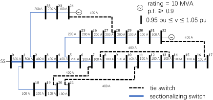
Figure 1: 33-bus distribution system from [1] with five tie-switches (dashed lines). Line width is proportional to current rating labeled next to the line.

We first attempt to solve the reconfiguration problem in (12) maximizing the total DG output with $K=0$ (i.e., OPF with original network topology). The instance is infeasible due to voltage restrictions. However, if we relax the voltage lower limit from 0.95 pu to 0.9 pu, the instance becomes feasible and the voltages from bus 12 to bus 17 (towards the end of the feeder) are below 0.95 pu. Next, we solve (12) with $K=2$ (i.e., one switch opened and another switch closed) with the usual voltage limits of 0.95 pu and 1.05 pu. The result is shown in Fig. 2, with a total DG output of 4.33 MW.

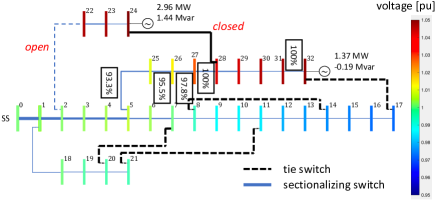
Figure 2: Reconfiguration with $K=2$ (line {2, 22} opened and line {24, 28} closed). Bus color shows the voltage level and the percentage of current rating of bottleneck lines are shown. Total DG output is 4.33 MW.

In this reconfiguration, switch $\{2,22\}$ is opened while switch $\{24,28\}$ is closed. This raises the voltages from bus 5 to bus 17, satisfying the lower limit of 0.95 pu (e.g., the voltage at bus 17 is 0.972 pu). If we re-solve (12) with $K=4$, the result is shown in Fig. 3, with total DG output increased to 5.67 MW.

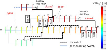
Figure 3: Reconfiguration with $K=4$ (lines {2, 22}, {28, 29} opened, and lines {24, 28}, {17, 32} closed). Bus color shows the voltage level and the percentage of current rating of bottleneck lines are shown. Total DG output is 5.67 MW.

With $K=4$, switch $\{28,29\}$ is opened while switch {17, 32} is closed, in addition to the topology adjustments made in the case of $K=2$. This prevents the two DG sources from sharing the path segment between bus 5 and bus 28, which is the bottleneck for $K=2$. If we further increase $K=6$ in (12), the outcome is to open {10, 11} and close {11, 21}, cutting short the feeder from bus 0 to bus 17. This increases the total DG output to 5.72 MW.

The aforementioned results help us to identify the segment between bus 5 and bus 28 to be the bottleneck. If we increase the current ratings of these four lines (e.g., due to dynamic line rating), we expect the DG output to further increase. Indeed, if the ratings are increased from 200 A to 300 A, then for $K=0,2,4,6$ the total DG outputs are, respectively, 0 MW (infeasible instance), 5.44 MW, 6.68 MW, and 6.77 MW.

III-B Computation Time Evaluation

The elapsed runtime to solve the benchmark instances is summarized in Table II.

TABLE II: Runtime [s] to achieve 0.01% optimality gap, or optimality gap [%] after one-hour runtime, for benchmark instances of (12)

name	$K=0$	$K=2$	$K=4$	$K=6$	$K=8$
33bw	N/A	1.56s	1.69s	2.21s	4.06s
118zh	0.82s	20.18s	28.7s	105.5s	275.74s
136ma	0.14s	4.88s	12s	15.35s	58.16s
REDS 29+1	0.12s	0.62s	0.61s	0.63s	1.38s
REDS 83+11	N/A	N/A	0.42s	2.33s	3.32s
REDS 135+1	0.12s	4.46s	19.82s	235.7s	1.99%
REDS 201+3	0.7s	13.43s	41.11s	88.76s	280.96s
REDS 873+7	5s	265s	1337s	3.38%	4.54%

In the table, N/A means that the instance is infeasible. In addition, for REDS 135+1 with $K=8$ and REDS 873+7 with $K=6$ and $K=8$ the table entries show the percentage optimality gap after time limit of one hour. In general, runtime increases as the network size and $K$ increase. However, there are exceptions as REDS 135+1 appears to be difficult for $K=8$ (cf. 136ma with $K=8$ differing only in DG locations), whereas REDS 83+11 is easy (even with $K=26$ the runtime is 11.8s, not shown in Table II). Despite some irregularities in the runtime pattern, we conclude that the proposed method can reliably obtain guaranteed optimal DG set points and network configuration for moderately-sized instances (e.g., networks up to few hundred buses and $K\leq 6$). However, discretion is needed when attempting to solve larger instances. Nevertheless, typically the marginal benefit diminishes rapidly with increasing $K$ [2]. Furthermore, despite not being able to solve large instances to optimality, the proposed method can return suboptimal solutions with certified optimality gap. Runtime to achieve 5% optimality gap for the benchmarks is summarized in Table III.

TABLE III: Runtime to achieve 5% optimality gap for benchmark instances of (12)

name	$K=0$	$K=2$	$K=4$	$K=6$	$K=8$
33bw	N/A	1.14s	1.32s	1.88s	3.92s
118zh	0.31s	14.28s	23.94s	61.93s	119.42s
136ma	0.14s	3.23s	10.87s	14.93s	37.22s
REDS 29+1	0.11s	0.61s	0.61s	0.63s	0.63s
REDS 83+11	N/A	N/A	0.27s	1.49s	3.04s
REDS 135+1	0.11s	3.09s	8.80s	5.96s	91.74s
REDS 201+3	0.30s	12.89s	39.41s	84.63s	241.36s
REDS 873+7	0.58s	86.87s	482.4s	1109s	1854s

III-C Comparison with Local Optimization Solvers

In this part of case study, we compare the OPF results by solving (12) with $K=0$ and by using Matpower 7.1’s OPF subroutine runopf.m. The Matpower OPF formulation is based on the AC power flow equations (voltage phasors in polar coordinates) instead of the DistFlow equations in (1) in the proposed model. To maximize the total DG output, the Matpower OPF cost function is set to $\sum_{n}c^{0}_{n}+c^{1}_{n}p_{n}^{G}+c^{2}_{n}(p_{n}^{G})^{2}$ with $c^{0}_{n}=c^{2}_{n}=0$ and $c^{1}_{n}=-1$ for all $n\in\mathcal{N}$. This is not the typical positive quadratic cost function. We run Matpower with the default options (e.g., flat start initial guess) and with two optimization solver choices: (a) MIPS interior point method and (b) Matlab’s fmincon active set method. For the feasible instances in Table II, Matpower OPF solves the benchmark OPF instances with relative ease except that MIPS fails to converge for the 201+3 case. However, Matpower OPF does not provide the optimality guarantee available in the proposed method. Furthermore, Matpower OPF results are sensitive to problem instance data and algorithmic choices. For example, if we increase line current ratings to 600 A for all lines and slightly decrease the DG ratings to 8 MW, the OPF instance for the 33bw benchmark becomes feasible but the Matpower OPF results vary greatly depending on the solver choice and initial guess strategy. Table IV shows the DG maximization results, where the Matpower initial guess strategies include: 0 for flat start, 1 for ignoring the system state (i.e., voltages and generation) in the Matpower case, 2a and 2b for using the system state in the Matpower case (without and with update by first solving (12)) and 3a and 3b for solving power flow and using the resulting state (without and with update by first solving (12)). Table IV indicates that local optimization methods implemented in Matpower cannot reliably solve the DG maximization problem. On the other hand, the proposed method yields the desired DG value of 10.45 MW. Further, we note that the difficulty exhibited in Table IV is intrinsic to the DG maximization objective (as in (12)). If we instead minimize $\sum_{n}c^{0}_{n}+c^{1}_{n}p_{n}^{G}+c^{2}_{n}(p_{n}^{G})^{2}$ with $c^{0}_{n}=c^{2}_{n}=0$ and $c^{1}_{n}=1$ (instead of $-1$) for all $n$, Matpower can reliably obtain the minimum total DG of 1.93 MW using both MIPS and fmincon for all choices of initial guess strategies.

TABLE IV: 33bw 600 A, Matpower OPF, max DG output

initial guess strategy	0	1	2a
MIPS	9.45 MW	9.45 MW	9.45 MW
fmincon	10.44 MW	10.44 MW	fail
initial guess strategy	2b	3a	3b
MIPS	10.44 MW	9.43 MW	10.44 MW
fmincon	fail	8.78 MW	fail

III-D Comparing Mixed Integer Conic Programming Relaxation

In this part of case study, we evaluate the mixed integer conic relaxation approach in (13). A central question regarding the use of (13) is whether (13) is tight (i.e., (13b) are satisfied as equalities at optimality). Here we present a counterexample: Consider the OPF problem for the three-bus example in Fig. 4.

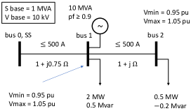
Figure 4: 3-bus distribution system example demonstrating failure of the relaxation approach. The voltage at bus 0 is 1 pu.

We use Gurobi to solve (12) and (13) with $K=0$ (using the same AMPL code except for the difference between (5d) and (13b) and the Gurobi “non-convex” option setting). The results are summarized in Table V, showing different values of DG outputs highlighted in red (indicating failure of conic relaxation).

TABLE V: Per unit OPF results for Fig. 4 by (12) and (13)

Bilinear program in (12)
bus	$\nu$	$\ell$	$p^{G}$	$q^{G}$	$P$	$Q$
1	1.1025	25	7.7518	0.39754	$-4.9991$	0.092606
2	1.0964	0.2645	0	0	0.50264	$-0.19736$
Conic relaxation in (13)
bus	$\nu$	$\ell$	$p^{G}$	$q^{G}$	$P$	$Q$
1	1.1025	25	7.9991	0.64489	$-4.9991$	0.092606
2	1.0915	25	0	0	0.75	0.049999

With the problem data in Fig. 4 and the variable values in Table V, we can verify that the solutions of (12) and (13) satisfy all constraints in the respective problems. For example, the reactive power balance equation in (1b) for bus 1 for (12) is $q^{G}_{1}-q^{L}_{1}=0.39754-0.5=-0.10246=(-1)\times 0.092606+(-0.19736)+0.0075\times 25=-Q_{1}+Q_{2}+x_{01}\ell_{1}$. The analogous equation holds for the solution of (13) as well: $q^{G}_{1}-q^{L}_{1}=0.64489-0.5=0.14489=(-1)\times 0.092606+0.049999+0.0075\times 25=-Q_{1}+Q_{2}+x_{01}\ell_{1}$. However, while equation (5d) at bus 2 holds for the solution of (12): $\nu_{1}\ell_{2}=1.1025\times 0.2645=0.2916=0.50264^{2}+{(-0.19736)}^{2}=P_{2}^{2}+Q_{2}^{2}$, (13b) remains an inequality instead of equality for the solution of (13): $\nu_{1}\ell_{2}=1.1025\times 25=27.5625>0.565=0.75^{2}+0.049999^{2}=P_{2}^{2}+Q_{2}^{2}$. Indeed, a posterior load flow analysis based on $(p^{G},q^{G})$ from (13) reveals that the bus voltages are 1, 1.0539 and 1.0511 per unit, respectively. Similarly, the currents for the lines are 522.53 A and 51.235 A. The voltage and current upper limits are both violated by the solution of conic relaxation. The aforementioned comparison is repeated for all benchmarks in Table I. The conic relaxation solutions fail to satisfy equality (5d) in all cases, and result in voltage and current violations.

The objective functions in (12) and (13) have a significant impact on the tightness of conic relaxation. For instance, if we instead minimize the total line loss (as in [2, 16]), then the solutions of (13) also solve (12) for all benchmark instances in Table I, except for the instances not achieving convergence within the time limit of one hour. Following [28], we consider the trade-off between DG maximization and line loss minimization by minimizing in (12) and (13) the following weighted sum objective:

$$\rho\sum\limits_{n\in\mathcal{N}}\big{(}\sum\limits_{k\in\bar{\mathcal{N}}}\pi_{kn}r_{kn}\big{)}\ell_{n}-(1-\rho)\sum\limits_{n\in\mathcal{N}}p^{G}_{n}$$ (14)

where $0\leq\rho\leq 1$ is an algorithmic parameter for trade-off. With $\rho$ increasing from 0 to 1, the minimization of (14) transitions from DG maximization to loss minimization. By solving (12) and (13) with (14) and running a posterior load flow analysis based on the resulting DG set points and network configuration, the trade-off can be visualized. Fig. 5 shows the Pareto curves for the 33bw benchmark with universal line rating of 600 A and $K=6$.

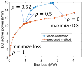
Figure 5: Pareto curves of 33bw benchmark (600A line rating) due to the proposed model in (12) and conic relaxation in (13)

For $\rho>0.5$, the two Pareto curves coincide since the conic relaxation solution satisfies (5d). However, when $\rho\leq 0.5$ conic relaxation fails, and conic relaxation no longer depicts the true trade-off. The extra “DG output” of conic relaxation is paid by violating the voltage and current limits. We note that the part of the Pareto curve of the proposed method for $\rho\leq 0.5$ is in fact not obtained by solving (12) with (14) but rather by maximizing DG as in (12) with an additional constraint upper bounding total line loss.

III-E Comparison with Linearized DistFlow Approximation

We evaluate a variant of (12) by replacing the DistFlow equations in (5) with its linear approximation (i.e., LinDistFlow equations [1]). The LinDistFlow variant ignores the loss-related terms multiplying $\ell_{n}$ in (5a), (5b) and (5c). Also, equation (5d) is dropped. Substituting the DistFlow equations with the LinDistFlow equations changes (12) to a mixed integer linear program, which is easier to solve. However, the voltage variables in the LinDistFlow variant overestimate the true voltages (e.g., [29, eq. (2a) and (3)]). This may lead to false voltage lower limit satisfaction. Further, since the squared current term $\ell$ is missing it is not possible to directly impose current upper limit constraints. Indeed, for our benchmark instances severe violation of current upper limit is experienced. To counter this, a surrogate current upper limit constraint can be imposed, similar to (5d), as

$$\Big{(}\sum\limits_{k\in\bar{\mathcal{N}}}\pi_{kn}\nu_{k}\Big{)}\Big{(}\sum\limits_{k\in\bar{\mathcal{N}}}\pi_{kn}\overline{\ell}_{kn}\Big{)}\geq P_{n}^{2}+Q_{n}^{2},\quad n\in\mathcal{N}$$ (15)

In (15) the product in the left-hand-side can be simplified using the linearization technique illustrated in (6). Below we call LinDistFlow the variant of (12) with LinDistFlow equations and (15). The inclusion of (15) relieves some undervoltage and overcurrent issues. However, this is not enough. For instance, for the 33bw benchmark with 600 A line rating and $K=2$, the actual voltages by a posterior load flow analysis and the voltages perceived to be true by the LinDistFlow optimization model (i.e., $(\nu)^{1/2}$) are very different as indicated by Fig. 6.

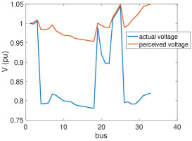
Figure 6: Benchmark 33bw (600 A line rating): actual voltage profile by a posterior load flow analysis and voltage profile perceived to be true by the LinDistFlow optimization model

Also, current upper limits are violated in multiple lines (worst case violation being 115% of rating) despite the surrogate constraint in (15). For LinDistFlow with $K=4$ the result is even more extreme. The load flow analysis by Matpower fails to converge. In contrast, solving (12) for the 33bw 600 A benchmark with $K=2$ and $K=4$, respectively, leads to constraint-abiding control with guaranteed optimality.

III-F Comparison with Equivalent Formulation by Jabr et. al.

We compare the proposed method with the reconfiguration formulation adopted from [2] by changing the objective from total line loss minimization to DG maximization. Almost all constraints in [2] are linear except

$$2u^{(n,k)}u^{(k,n)}\geq R_{nk}^{2}+T_{nk}^{2},\quad\text{$\{n,k\}$ is a line}$$ (16)

In (16), all symbols are continuous decision variables and hence (16) are rotated second order cone inequalities. In fact, (16) is a relaxation. The model in [2] is equivalent to (12) only when (16) hold as equalities. Similar to conic relaxation discussed in Section III-D, when minimizing a “standard” objective such as total line loss the inequalities in (16) are often satisfied as equalities at optimality. However, for DG maximization (16) remain inequalities and the resulting control violates voltage and current limits. For example, for the 33bw benchmark with 600 A line rating, solving the formulation in [2] with $K=4$ leads to voltage violation up to 1.25 pu and current violation up to 137% of line rating. To rectify the situation, we can impose (16) as equalities. However, imposing (16) as equalities renders the formulation in [2] very difficult to solve. For instance, for 33bw with a 300-second time limit Gurobi terminates with optimality gap of 256%, 287%, 342% and 205% for $K=2,4,6,8$, respectively (cf. Table II).

IV Case Study - Real Network

IV-A 533-bus Distribution System Description

In this section, the ROPF problem (12) is applied to a real medium voltage distribution system in southern Sweden: the 533-bus network described in [30]. With the expansion of distributed energy resources (DERs), many DSOs wish to assess to what extent DERs can be integrated in their systems without violating operational limits. This is referred to as performing a hosting capacity (HC) analysis. In [31], four operational limits that constrain the HC in distribution networks are outlined – voltage, overloading, protection and harmonics. With our proposed method we are imposing voltage and current limits, thereby dealing with the first two. Protection is partly included by requiring radial operation, but no further protection limits (i.e. short-circuit current) are set up. The system is assumed to be three-phase balanced without overtones, thus harmonics mitigation is not considered. Within these limits, the HC can be assessed and enhanced, using e.g. network reconfiguration, and our proposed ROPF method does this jointly.

The network in [30] operates at 12 kV with a smaller part at 135 kV, covers about 20$\times$30 km and serves about 30,000 inhabitants plus an industrial area. It is connected to the regional 135 kV grid at a single feed-in station, modeled as a slack bus. A system overview is seen in Fig. 7.

Figure 7: Map of the 533-bus distribution system. The width of each line is proportional to its rated current.

The system contains 533 nodes and 577 lines, thus radial operation (3c) requires that 45 lines are always disconnected. Although a disconnected line might still be energized, the existence of an open point renders the entire line topologically switched off. The normal radial topology, used as base case ($K=0$) for subsequent simulations, can be seen in Fig. 8.

The existing wind and solar DG capacity amounts to 34.5 MW, installed at 262 nodes with capacities ranging from 3 kW to 2 MW per node. To avoid curtailment of already existing DG in the system, production from existing DG is embedded in $p^{L}_{n}$ by subtracting hourly generation from hourly load to obtain the net load data for each node. In the year 2022, the total net load in the system varied from 44.6 MW in Dec 16, 08:00 to -4.8 MW in Jul 10, 14:00. The latter will be referred to as the minimum net load hour.

The voltage constraints in (8) are set to $\sqrt{\underline{\nu_{n}}}=0.95$ pu and $\sqrt{\overline{\nu_{n}}}=1.05$ pu, whereas the current constraints $\overline{\ell_{kn}}$ in (9) are set individually for each line, according to their respective rated currents. All system data was provided by the DSO. In the real network, there are often several line segments and conductor types connecting two substations, while in the model these are aggregated to single lines with equivalent rated currents and impedances. A full description of this aggregation procedure can be found in [30]. Once the aggregation has been made, the single lines have rated phase currents ranging from 93-1200 A, phase resistances from 0.003-1.86 $\Omega$ and phase reactances from 0.001-0.73 $\Omega$.

Furthermore, the real network is a three-phase system, whereas the optimization algorithm is designed for single-phase. Since the system is assumed to be three-phase balanced, this was managed by dividing all loads and generation capacities by a factor three, effectively treating each phase as a separate system. After simulations were run, the actual power flows were obtained by multiplying all power values post-optimization with a factor three.

The final Matpower-model of the 533-bus system can be found at github.com/MATPOWER/matpower/blob/master/data/case533mt_lo.m with net load values from the minimum net load hour.

IV-B Reconfiguration with 533-bus Example

The ROPF problem in (12) is solved for the 533-bus system through two separate case studies. The first study involves the construction of a multiple node generation scenario, representing a potential future expansion of wind power. The second study is a spatially comprehensive DG expansion site analysis, where additional DG capacity is added only to a single node in the system at the time, but iterating through the entire system, to see how high the HC is in each specific location and how much it can be increased through network reconfiguration.

In both the wind scenario and the DG expansion site analysis, the problem is solved with the minimum net load hour of 2022 as load input. The minimum net load hour is considered to be a good worst-case scenario, since bus voltages throughout the network are high during this hour and overvoltage is frequently the HC limiting factor.

IV-B1 Wind scenario

In the wind scenario, DG units of 2 MW are added to 21 rural nodes in clusters of up to four units. The placement of these clusters can be seen in Fig. 8. The clusters are added without grid expansion or reinforcement, to determine the HC of the existing grid, before and after reconfiguration. Note that the 21 wind units are the only $p^{G}_{n}$ in the optimization, since existing DG is embedded in $p^{L}_{n}$.

Figure 8: Setup of the wind scenario in the normal radial topology. Green circles display the 21 nodes where additional DG units of 2 MW have been placed.

Solving (12) for this generation setup, $\sum_{n}p^{G}_{n}=17.6$, $19.2$ and $19.3$ MW for $K=0$, $2$ and $4$ respectively. As an initial observation, the added DG capacity of $21\times 2=42$ MW is significantly curtailed both with and without reconfiguration. With $K=2$, the HC increases by 1.6 MW (or 9.1%) compared to the normal topology. This increase is due to a pair of switch events that divides a cluster of four units in the southeast on two separate feeder lines, in contrast to the normal topology where they share a common feeder that turns out to be a bottleneck (see Fig. 9 and Fig. 10). If four switch events are allowed ($K=4$), the algorithm returns the same first pair of switch events as with $K=2$, but also another pair of switch events closer to the distribution station LF. This has a more limited effect, increasing HC by only 0.1 MW from $K=2$.

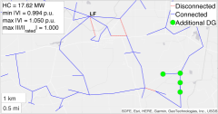
Figure 9: Wind scenario in the normal radial topology ($K=0$), zoomed in at the southeastern part of the network.

Figure 10: Wind scenario after reconfiguration ($K=2$),
the black arrows indicate where switch events occurred.

IV-B2 DG expansion site analysis

In the DG expansion site analysis, additional DG capacity is added to a single node one at a time. This added capacity is large enough for the apparent power rating of the unit to not be an active constraint in (7b), allowing us to identify the HC of the grid. After adding DG to a single node, (12) is solved with $K=0$, $2$ and $4$, to enable a comparison of the HC before and after reconfiguration. This procedure is repeated for all 532 non-slack nodes in the system, sometimes referred to as the iterative or detailed method [32]. No single optimization took more than 10 mins, which is considered reasonable for a site analysis.

In Fig. 11, the results from the $532\times 3$ optimizations in the DG expansion site analysis can be seen. The $x,y$-value indicates the location of a node in the network and the bar height is the HC at that node in MW. The blue part of each bar is the HC in the normal radial topology, whereas the red and yellow part is the additional HC including reconfiguration with $K=2$ and $4$ respectively.

Figure 11: 3D bar chart displaying the HC at each node. The blue, red and yellow parts are with $K=0$, $2$ and $4$ respectively.

Tall bars in Fig. 11 indicate a high HC, typically found at distribution substations or large industry nodes. On average, the HC is also higher at urban nodes than at rural. A large share of red or yellow in a bar indicates that the HC at that node can be improved substantially by reconfiguration. A large share of the urban nodes, but also some rural, exhibit this substantial increase in HC from reconfiguration.

In Fig. 12, these relative HC improvements from network reconfiguration are presented explicitly. The figure displays how many of the nodes, $x\%$, that exhibit a relative HC increase of $y\%$ or higher from reconfiguration.

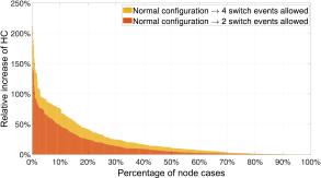
Figure 12: Share of nodes, $x\%$, that exhibit a HC increase of $y\%$ or higher from reconfiguration. Red depict the increase from $K=0$ to $K=2$, yellow from $K=0$ to $K=4$.

Fig. 12 shows that the potential to enhance the HC through network reconfiguration varies considerably between nodes. The location of a node, and the network topology in its vicinity, has a significant effect on the benefit that can be achieved from reconfiguration. The greatest increase from $K=0$ to $K=4$ is as high as 212% for a single node. Meanwhile, the median increase from $K=0$ to $K=4$ is only about 11%.

IV-C Discussion of 533-bus Example

The results from this section show that our proposed method can be used to address relevant problems that many DSOs today are facing. The wind scenario shows that the ROPF method can return new, more beneficial topologies for DG expansion. All else equal, our proposed method can thus reduce the need for costly network expansion/reinforcement. The DG expansion site analysis demonstrates how our proposed method can be used to assess and enhance the HC at specific sites. In particular, this can be done with reconfiguration taken into account, adding an additional feature to classic OPF.

Due to local variations and other complicating factors, it is far from certain that the HC is always most limited during the minimum net load hour. The results from this section should thus be interpreted as proof of concept and areas of use of our proposed method, rather than as a comprehensive HC analysis of this particular system.

V Conclusion

DG maximization is more difficult than loss reduction for network reconfiguration as the former objective renders standard techniques such as local optimization, conic relaxation and linearization approximation ineffective, thus raising caution against their over-generalization and highlighting the importance of decision models featuring exact AC power flow equations (or equivalents). With today’s optimization technology, the DG maximization problem can be handled reasonably well for moderately sized networks in a time scale relevant for control center applications. The ability to handle exact AC power flow constraints helps not only in network reconfiguration but also in parameter estimation, fault detection and contingency analysis. However, experiments are needed to evaluate the computation performance in these use cases. On another note, the DistFlow equations appear to be “easier constraints” than other equivalents such as AC power flow equations and the expression in [2]. The effect of problem formulations on branch-and-bound algorithm performance is not well understood. Insights on the effect are highly desirable.

References

- [1] M. E. Baran and F. F. Wu, “Network reconfiguration in distribution systems for loss reduction and load balancing,” IEEE Power Engineering Review, vol. 9, no. 4, pp. 101–102, 1989.
- [2] R. A. Jabr, R. Singh, and B. C. Pal, “Minimum loss network reconfiguration using mixed-integer convex programming,” IEEE Transactions on Power systems, vol. 27, no. 2, pp. 1106–1115, 2012.
- [3] Y. Song, Y. Zheng, T. Liu, S. Lei, and D. J. Hill, “A new formulation of distribution network reconfiguration for reducing the voltage volatility induced by distributed generation,” IEEE Transactions on Power Systems, vol. 35, no. 1, pp. 496–507, 2019.
- [4] F. Capitanescu, L. F. Ochoa, H. Margossian, and N. D. Hatziargyriou, “Assessing the potential of network reconfiguration to improve distributed generation hosting capacity in active distribution systems,” IEEE Transactions on Power Systems, vol. 30, no. 1, pp. 346–356, 2014.
- [5] T. Yang, Y. Guo, L. Deng, H. Sun, and W. Wu, “A linear branch flow model for radial distribution networks and its application to reactive power optimization and network reconfiguration,” IEEE Transactions on Smart Grid, vol. 12, no. 3, pp. 2027–2036, 2020.
- [6] Y.-Y. Fu and H.-D. Chiang, “Toward optimal multiperiod network reconfiguration for increasing the hosting capacity of distribution networks,” IEEE Transactions on Power Delivery, vol. 33, no. 5, 2018.
- [7] C. Ababei and R. Kavasseri, “Efficient network reconfiguration using minimum cost maximum flow-based branch exchanges and random walks-based loss estimations,” IEEE Transactions on Power Systems, vol. 26, no. 1, pp. 30–37, 2010.
- [8] K. W. Hedman, S. S. Oren, and R. P. O’Neill, “A review of transmission switching and network topology optimization,” in 2011 IEEE power and energy society general meeting. IEEE, 2011, pp. 1–7.
- [9] C.-T. Su and C.-S. Lee, “Network reconfiguration of distribution systems using improved mixed-integer hybrid differential evolution,” IEEE Transactions on power delivery, vol. 18, no. 3, pp. 1022–1027, 2003.
- [10] D. Zhang, Z. Fu, and L. Zhang, “An improved ts algorithm for loss-minimum reconfiguration in large-scale distribution systems,” Electric power systems research, vol. 77, no. 5-6, pp. 685–694, 2007.
- [11] E. R. Ramos, A. G. Expósito, J. R. Santos, and F. L. Iborra, “Path-based distribution network modeling: application to reconfiguration for loss reduction,” IEEE Transactions on power systems, vol. 20, no. 2, pp. 556–564, 2005.
- [12] E. B. Fisher, R. P. O’Neill, and M. C. Ferris, “Optimal transmission switching,” IEEE Transactions on Power Systems, vol. 23, no. 3, pp. 1346–1355, 2008.
- [13] H. Ergun, D. Van Hertem, and R. Belmans, “Transmission system topology optimization for large-scale offshore wind integration,” IEEE Transactions on Sustainable Energy, vol. 3, no. 4, pp. 908–917, 2012.
- [14] M. K. Singh, S. Taheri, V. Kekatos, K. P. Schneider, and C.-C. Liu, “Joint grid topology reconfiguration and design of watt-var curves for ders,” in 2022 IEEE Power & Energy Society General Meeting (PESGM). IEEE, 2022, pp. 1–5.
- [15] M. Farivar and S. H. Low, “Branch flow model: Relaxations and convexification – Part I,” IEEE Transactions on Power Systems, vol. 28, no. 3, pp. 2554–2564, 2013.
- [16] J. A. Taylor and F. S. Hover, “Convex models of distribution system reconfiguration,” IEEE Transactions on Power Systems, vol. 27, no. 3, pp. 1407–1413, 2012.
- [17] B. Kocuk, S. S. Dey, and X. A. Sun, “New formulation and strong misocp relaxations for ac optimal transmission switching problem,” IEEE Transactions on Power Systems, vol. 32, no. 6, pp. 4161–4170, 2017.
- [18] C. Lee, C. Liu, S. Mehrotra, and Z. Bie, “Robust distribution network reconfiguration,” IEEE Transactions on Smart Grid, vol. 6, no. 2, pp. 836–842, 2014.
- [19] J. M. Home-Ortiz, L. H. Macedo, R. Vargas, R. Romero, J. R. S. Mantovani, and J. P. Catalão, “Increasing res hosting capacity in distribution networks through closed-loop reconfiguration and volt/var control,” IEEE Transactions on Industry Applications, vol. 58, no. 4, pp. 4424–4435, 2022.
- [20] M. Čičić, C. Vivas, C. C. de Wit, and F. Rubio, “Optimal renewable energy curtailment minimization control using a combined electromobility and grid model,” in IFAC 2023-The 22nd World Congress of the International Federation of Automatic Control, 2023.
- [21] R. D. Zimmerman, C. E. Murillo-Sánchez, and R. J. Thomas, “Matpower: Steady-state operations, planning, and analysis tools for power systems research and education,” IEEE Transactions on power systems, vol. 26, no. 1, pp. 12–19, 2010.
- [22] R. Horst and H. Tuy, Global optimization: Deterministic approaches. Springer Science & Business Media, 2013.
- [23] K. C. Sou and J. Lu, “Relaxed connected dominating set problem for power system cyber–physical security,” IEEE Transactions on Control of Network Systems, vol. 9, no. 4, pp. 1780–1792, 2022.
- [24] K. C. Sou and K. Girón, “Joint renewable generation maximization and radial distribution network reconfiguration,” in 2022 IEEE PES Innovative Smart Grid Technologies-Asia (ISGT Asia), pp. 16–20.
- [25] S. P. Boyd and L. Vandenberghe, Convex optimization. Cambridge university press, 2004.
- [26] W. Wei, J. Wang, N. Li, and S. Mei, “Optimal power flow of radial networks and its variations: A sequential convex optimization approach,” IEEE Transactions on Smart Grid, vol. 8, no. 6, pp. 2974–2987, 2017.
- [27] M. A. Guimaraes and C. A. Castro, “Reconfiguration of distribution systems for loss reduction using tabu search,” in IEEE Power System Computation Conference (PSCC), vol. 1, 2005, pp. 1–6.
- [28] R. Cadjenovic and D. Jakus, “Maximization of distribution network hosting capacity through optimal grid reconfiguration and distributed generation capacity allocation/control,” Energies, vol. 13, no. 20, p. 5315, 2020.
- [29] K. C. Sou and H. Sandberg, “Resilient scheduling of control software updates in radial power distribution systems,” IEEE Transactions on Control of Network Systems, 2023. [Online]. Available: https://doi.org/10.1109/TCNS.2023.3338254
- [30] G. Malmer and L. Thorin, “Network reconfiguration for renewable generation maximization,” Master’s thesis, Lund University, 2023.
- [31] S. M. Ismael, S. H. Abdel Aleem, A. Y. Abdelaziz, and A. F. Zobaa, “State-of-the-art of hosting capacity in modern power systems with distributed generation,” Renewable Energy, vol. 130, pp. 1002–1020, 2019.
- [32] S. Stanfield, S. Safdi, S. Mihaly, and L. Weinberger, “Optimizing the grid: A regulator’s guide to hosting capacity analyses for distributed energy resources,” Interstate Renewable Energy Council, Tech. Rep., 2017.