Deep-Learning-Based Channel Estimation for Distributed MIMO with 1-bit Radio-Over-Fiber Fronthaul
Abstract
We consider the problem of pilot-aided, uplink channel estimation in a distributed massive multiple-input multiple-output (MIMO) architecture, in which the access points are connected to a central processing unit via fiber-optical fronthaul links, carrying a two-level-quantized version of the received analog radio-frequency signal. We adapt to this architecture the deep-learning-based channel-estimation algorithm recently proposed by Nguyen et al. (2023), and explore its robustness to the additional signal distortions (beyond -bit quantization) introduced in the considered architecture by the automatic gain controllers (AGCs) and by the comparators. These components are used at the access points to generate the two-level analog waveform from the received signal. Via simulation results, we illustrate that the proposed channel-estimation method outperforms significantly the Bussgang linear minimum mean-square error channel estimator, and it is robust against the additional impairments introduced by the AGCs and the comparators.
I Introduction
In distributed massive multiple-input multiple-output (MIMO), a large number of remotely located access points (APs) serve a much smaller number of user equipments (UEs) in a coordinated way. Coordination is enabled by a central processing unit (CPU), which is connected to the APs via fronthaul links. With such an architecture, one can exploit macro-diversity and mitigate path-loss variations compared to co-located massive MIMO architectures. This yields a more uniform quality of service [1].
In the analysis of distributed MIMO systems, it is often assumed that the APs are equipped with local oscillators, which are used for up- and down-conversion, and that samples of the base-band (BB) signals are exchanged between the APs and the CPU over the fronthaul links. However, these local oscillators need to be synchronized for reciprocity-based joint coherent downlink beamforming to work, which may be costly or even unfeasible in certain deployments [2].
To solve this issue, an alternative architecture has been proposed in the literature (see, e.g., [3, 4, 5, 6, 7]), in which up- and down-conversion are performed digitally at the CPU. This, however, implies that radio frequency (RF) signals need to be exchanged over the fronthaul links. To limit complexity and fronthaul requirements, in the architecture proposed in [3, 4, 5, 6, 7], only a two-level representation of the RF signal is exchanged over the fronthaul link. This implies that quantizers with just a single-bit resolution can be deployed at the CPU. The testbed measurements reported in, e.g., [6, 7] demonstrate that satisfactory performance can be achieved despite the nonlinearities introduced by this architecture, provided that the -bit quantizers at the CPU operate at a sufficiently high sampling rate—roughly two orders of magnitude larger than the bandwidth of the transmitted signal.
This paper focuses on the problem of acquiring accurate channel estimates via uplink pilot transmission, to enable reciprocity-based coherent downlink beamforming. The problem of channel estimation in the presence of the impairments caused by -bit quantization is well-studied in the literature, although most works focus on the scenario in which sampling is performed on the BB signal and not the RF signal. Relevant contributions involve the derivation of the linear minimum mean-squared error (LMMSE) estimator via Bussgang decomposition [8] as well as of methods for the efficient evaluation of the maximum a posteriori and maximum likelihood (ML) channel estimators, by exploiting the convexity of the log-likelihood functions [9, 10]. More recently, several methods relying on deep neural networks have been proposed in the literature (see, e.g., [11] and references therein).
In this paper, we will focus on the machine-learning algorithm proposed in [11], where deep unfolding of the iterations of a first-order optimization method is used to tackle the ML channel-estimation problem. Specifically, we adapt the algorithm proposed in [11] to the 1-bit radio-over-fiber fronthaul architecture considered in this paper. Our extension accounts for the real-valued nature of the sampled signals, and for oversampling and dithering. Furthermore, we analyze the robustness of the resulting algorithm to the additional impairments introduced in our architecture by the automatic gain controller (AGC), which limits the range of the received signal power at which dithering is effective, and by the comparator, which introduces random bit flips when the difference between the signals at its input ports is small.
II System Model
II-A Distributed MIMO with 1-Bit Radio-Over-Fiber Fronthaul
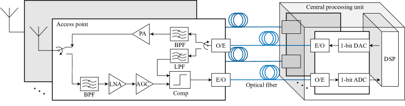
In Fig. 1, we illustrate the key components of the distributed MIMO architecture with 1-bit radio-over-fiber fronthaul, and single-antenna APs, described in [6, 7].
Downlink
In the downlink, modulated and precoded BB signals intended for the UEs are up-converted digitally to the carrier frequency at the CPU, and then band-pass (BP) sigma-delta modulated. This yields an oversampled binary representation of the RF signals. Sigma-delta modulation relies on oversampling and noise shaping to place the quantization distortion outside the bandwidth of the desired signal [12]. Analog signals are then generated via 1-bit digital-to-analog converters (DACs). Subsequently, these signals are converted into the optical domain by electrical-to-optical (E/O) converters and conveyed to the desired APs via optical fibers. A reconstruction band-pass filter (BPF) at the AP suppresses the out-of-band distortion produced by the sigma-delta modulator and recovers the underlying (unquantized) RF waveform, which is then transmitted over the single antenna of each AP.
Uplink
The signal received at the antenna port of each AP is fed to a BPF and then passed through a low noise amplifier (LNA) and an AGC. The output of the AGC is fed to the positive differential input port of a comparator (denoted in the figure by “Comp”). The negative differential input port of the comparator is fed with a dither signal, which is provided to the AP via the downlink fiber-optical fronthaul. Specifically, this dither signal is generated digitally at the CPU, sigma-delta modulated, and recovered at the AP via a low-pass filter (LPF). The AGC has the important function to regulate the power of the received signal, in order to make dithering effective. The output of the comparator is converted into the optical domain and then conveyed to the CPU, where it is converted back to the electrical domain and then digitalized via a -bit analog-to-digital converter (ADC). The resulting samples are then digitally down-converted and further processed at the digital signal processing (DSP) unit.
II-B Pilot-Aided Channel Estimation: a Mathematical Model
We next consider the problem of uplink pilot-based channel estimation in the distributed MIMO architecture described in Fig. 1, and provide a mathematical model for the received signal, which we will use in Section III to generalize the channel-estimation algorithm proposed in [11].
To keep the notation compact, we will focus on the problem of estimating the channel between one arbitrary AP and UEs.111The mathematical model we provide in this section can be readily extended to the joint estimation of the channel between an arbitrary number of APs and UEs. However, such generalization appears to be superfluous, since, in distributed MIMO, the channels corresponding to different APs are typically assumed to be independent.
We assume that the UEs transmit pilot signals of bandwidth , centered at a frequency . We let denote the sampling rate at the ADCs and also assume that pilot transmission involves signals (where, as we shall see, is related to the number of pilot symbols transmitted per UE) of duration seconds, for some integer . Under these assumptions, we can write the resulting samples at the output of the -bit ADC as
| (1) |
Here, the matrix contains the samples of the discrete-time RF signal received at the AP (after the BPF), taken at the sampling frequency ; the matrix contains the samples of the dither signal added at the AP; finally, denotes the sign function, which models -bit quantization, and is applied entrywise to the matrix . For analytical convenience, we shall model the entries of the dither-signal matrix as independent random variables. Furthermore, we model as
| (2) |
where the -dimensional vector , whose th entry is given by , , models the up-conversion operation, and is the complex envelope of the discrete-time received signal.
We let , and assume for simplicity that is an odd integer. Furthermore, we define the following set:
| (3) |
To account for oversampling, we model as
| (4) |
Here, the matrix contains the channel coefficients (expressed in the frequency domain) that need to be estimated; the matrix contains the pilot symbols, which we assume have power ; the matrix , whose entries are drawn independently from a distribution, denotes the additive Gaussian noise; finally, the matrix is a truncated inverse discrete Fourier transform (IDFT) matrix, obtained by removing all columns of a IDFT matrix whose indices do not belong to the set defined in (3). Note that, in our notation, the oversampling ratio is given by .
It will turn out convenient to vectorize the matrix in (1). Specifically, we set . Similarly, we vectorize also , , , , and , obtaining the vectors , , , , and . Using this notation, we can equivalently express (2) and (4) as
| (5) |
and
| (6) |
Here, , , and , where indicates the Kronecker product. To summarize, we can compactly express the output signal in vectorized form as
| (7) |
III Deep-Learning-Based Channel Estimation
III-A Maximum-Likelihood Channel Estimation
We start by noting that the input–output relation (7) contains two random vectors, i.e., and . The entries of are correlated, which makes calculating the ML estimator mathematically difficult. To work around this problem, we ignore the additive noise vector while deriving the ML solution to the channel estimation problem.222The impact of this assumption will be discussed in Section V. Let
| (8) |
Then, by ignoring , we can write (7) as
| (9) |
Let be the conditional probability of in (9) given . Then the ML channel estimate is given by
| (10) | |||||
Here, denotes the cumulative distribution function of the normal distribution, , and denote the upper and lower thresholds of the quantization bin to which the th entry of the vector belongs.
It is now crucial to realize that the optimization problem in (10) is convex [11], [13], [10]. Let be the objective function in (10). Since is convex, we can solve (10) via an iterative gradient descent algorithm. However, the gradient of is undefined at certain points [11]. In addition, a lack of a closed-form expression for makes the optimization process more involved. To address these problems, we follow [11] and approximate as
| (11) |
with . Using (11), we can approximate as
| (12) | |||||
To perform iterative gradient descent on , we need to compute the vector-valued Wirtinger derivative [14, Cor. 5.0.1]
| (13) | |||||
Note that
| (14) | |||||
| (15) | |||||
where is applied element-wise to its vector-valued input.
We can now write the iterative gradient descent algorithm for minimizing the objective function as
| (16) |
where is the current iteration index and is the step size.
III-B Structure of the deep neural network (DNN)
Following [11], we use the deep unfolding technique [15] to implement each iteration of (16) as a DNN layer. Each layer of the network receives and calculates the gradient in (16) as
| (17) |
where and are the trainable parameters in the th layer. Note that the constants and in (15) are absorbed into the trainable parameters in (17). Training and corresponds to learning the step size and controlling the accuracy of the approximation in (11).
IV Refined System Model
As pointed out in [7, Figs. 11 and 12], the input/output relation in (7) does not match measurement results, since it ignores the impact of the AGC in the architecture presented in Fig. 1, as well as the distortion introduced by the comparator. In this section, we enhance the system model in (7) to include the effect of these two components.
AGC
The AGC is implemented in [7] via a feedback-controlled variable gain amplifier, which maintains the output power at within a dynamic range. Specifically, the maximum gain of the AGC is . Let be the average power of . We model the variable gain in introduced by the AGC as
| (18) |
The input to the comparator can then be modeled as , where .
Comparator
As discussed in [7], the comparator in Fig. 1 produces a lowpass-filtered version of a two-level waveform, because of its bandwidth limitations. As illustrated in [7, Fig. 12], when the synthesized waveform deviates significantly from the expected two-level waveform, the bits at the output of the ADCs are essentially generated at random, due to limitations in the decision circuitry. Typically, this occurs whenever the magnitude of the signal at the input of the comparator is small. To model this effect, we let be a diagonal matrix whose diagonal entries are drawn uniformly at random from the set if the corresponding entry of the vector is smaller in absolute value than a threshold , and are set to otherwise. In our simulations, we set , because this value matches the measurements reported in [7].
To summarize, in the proposed refined system model, the input–output relation (7) is replaced by
| (19) |
V Simulation Results
Simulation Parameters
Throughout this section, we assume that a single UE () transmits pilot symbols with power to the AP. We also assume that MHz, GHz, GS/s, , and . Finally, we let . The DNN used for channel estimation consists of layers. Denoting , we take as loss function the norm of . We use the Adam optimizer [16] with a learning rate that starts at and is multiplied by after every training epochs. The size of each training batch is , and the number of training epochs is . The performance metric used to evaluate and compare the channel estimation performance is the normalized mean square error (NMSE) averaged over channel realizations. The initial values for and are and , respectively. Furthermore, .
In Table I, we summarize the three different system models that are used for evaluating the performance of the proposed channel estimation algorithm.
Impact of Dithering
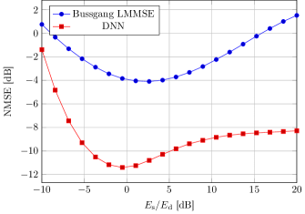
We start by considering Model 1, where we ignore the additive noise , and investigate the impact of the dither signal on the NMSE. The network is trained for values, uniformly spaced in the interval . The results are shown in Fig. 2. We see that, for Model 1, the proposed DNN-based channel estimator outperforms the Bussgang LMMSE estimator by at least , and that for our algorithm, the NMSE is minimized when . At this optimal value of , the performance gain of the proposed DNN-based channel estimator is around .
Impact of Additive Noise
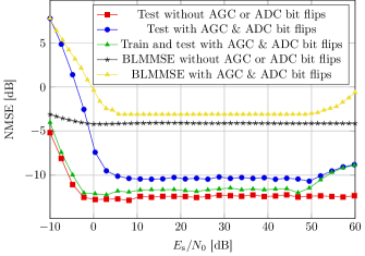
Next, we evaluate the test performance of a DNN trained at the optimal value in Fig. 2 using Model 1, for the case in which the test samples are generated according to Model 2. In Fig. 3 we show the NMSE as a function of . We observe that ignoring the additive noise during the training phase of the DNN (red curve) does not degrade its performance when noise is present. Indeed, the achieved NMSE value is in agreement with the optimal value reported in Fig. 2 for sufficiently large . We also observe that our DNN-based ML estimator outperforms the Bussgang LMMSE (black curve) by around when additive noise is present.
Impact of AGC and Random Bit Flips
Next, we investigate the impact of the additional impairments described in Section IV. We consider two additional scenarios: i) We test the trained DNN at the optimal obtained from Fig. 2 using Model 1 on a dataset generated from Model 3. ii) We train the DNN on datasets generated using Model 3, by considering values, spaced uniformly in the interval ; the ratio is still chosen according to Fig. 2. Then, we test each trained DNN on a new dataset generated from Model 3 using the same .
The NMSE achieved for these two additional scenarios is also shown in Fig. 3. We first notice that the DNN network trained on the dataset that does not take into account the effects of the AGC and ADC random bit flips (blue curve) performs poorly when is below or above . Indeed, in agreement with (18), outside this interval, the AGC cannot enforce the optimal signal-to-dither ratio. Furthermore, within the dynamic range of the AGC, we still see around performance degradation compared to the case when Model 2 is used (red curve), due to the effect of the random bit flips. Nevertheless, its performance is still superior to the one achievable using the Bussgang LMMSE (yellow curve) for the same scenario.
Interestingly, we also see that if we train the DNN on data generated according to the refined input–output relation (19) (green curve), the performance is significantly increased, despite the DNN possessing only trainable parameters, and despite the impairments not been explicitly modeled when deriving the gradient update step.
VI Conclusions
We have considered the problem of pilot-based uplink channel estimation in the distributed MIMO -bit radio-over-fiber architecture recently demonstrated in [7]. Specifically, we have adapted to this architecture the deep-unfolding-based ML channel estimation algorithm recently proposed in [11], and analyzed its robustness to the additional impairments introduced in the considered architecture by the AGC (dynamic range) and the comparator (random bit flips). In future works, we will measure over-the-air the performance achievable with the proposed algorithm using the testbed described in [7], and explore additional data-driven methods for channel estimation and data detection.
References
- [1] Ö. T. Demir, E. Björnson, and L. Sanguinetti, Foundations of user centric cell-free massive MIMO, ser. Foundations and Trends in Signal Processing. now Publishers, 2020, vol. 14, no. 3-4.
- [2] E. G. Larsson, “Massive synchrony in distributed antenna systems,” IEEE Trans. Signal Process., pp. 855–866, Jan. 2024.
- [3] R. F. Cordeiro, A. Prata, A. S. Oliveira, J. M. Vieira, and N. B. De Carvalho, “Agile all-digital RF transceiver implemented in FPGA,” IEEE Trans. Microw. Theory Techn., vol. 65, no. 11, pp. 4229–4240, Nov. 2017.
- [4] J. Wang, Z. Jia, L. A. Campos, and C. Knittle, “Delta-Sigma modulation for next generation fronthaul interface,” J. Lightw. Technol., vol. 37, no. 12, pp. 2838–2850, Jun. 2019.
- [5] C.-Y. Wu, H. Li, O. Caytan, J. Van Kerrebrouck, L. Breyne, J. Bauwelinck, P. Demeester, and G. Torfs, “Distributed multi-user MIMO transmission using real-time Sigma- Delta-over-fiber for next generation fronthaul interface,” J. Lightw. Technol., vol. 38, no. 4, pp. 705–713, Feb. 2020.
- [6] I. C. Sezgin, L. Aabel, S. Jacobsson, G. Durisi, Z. S. He, and C. Fager, “All-digital, radio-over-fiber, communication link architecture for time-division duplex distributed antenna system,” J. Lightw. Technol., vol. 39, no. 9, pp. 2769–2779, Feb. 2021.
- [7] L. Aabel, S. Jacobsson, M. Coldrey, F. Olofsson, G. Durisi, and C. Fager, “A TDD distributed MIMO testbed using a 1-bit radio-over-fiber fronthaul architecture,” IEEE Trans. Microw. Theory Tech., 2024.
- [8] Y. Li, C. Tao, G. Seco-Granados, A. Mezghani, A. L. Swindlehurst, and L. Liu, “Channel estimation and performance analysis of one-bit massive MIMO systems,” IEEE Trans. Signal Process., vol. 65, no. 15, pp. 4075–4089, Aug. 2017.
- [9] J. Choi, J. Mo, and R. W. Heath Jr, “Near maximum-likelihood detector and channel estimator for uplink multiuser massive MIMO systems with one-bit ADCs,” IEEE Trans. Commun., vol. 64, no. 5, pp. 2005–2018, May 2016.
- [10] C. Studer and G. Durisi, “Quantized massive MU-MIMO-OFDM uplink,” IEEE Trans. Commun., vol. 64, no. 6, pp. 2387–2399, Jun. 2016.
- [11] L. V. Nguyen, D. H. N. Nguyen, and A. L. Swindlehurst, “Deep learning for estimation and pilot signal design in few-bit massive MIMO systems,” IEEE Trans. Wireless Commun., vol. 22, no. 1, pp. 379–392, Jan. 2023.
- [12] S. Pavan, R. Schreier, and G. C. Temes, Understanding Delta-Sigma Data Converters, 2nd ed., R. Jacob Baker, Ed. Hoboken, NJ, USA: John Wiley & Sons, 2017.
- [13] J. W. Pratt, “Concavity of the log likelihood,” Journal of the American Statistical Association, vol. 76, no. 373, pp. 103–106, 1981.
- [14] R. Hunger, “An introduction to complex differentials and complex differentiability,” 2007. [Online]. Available: https://mediatum.ub.tum.de/doc/631019/631019.pdf
- [15] J. R. Hershey, J. L. Roux, and F. Weninger, “Deep unfolding: Model-based inspiration of novel deep architectures,” arXiv:1412.6980, 2009. [Online]. Available: https://arxiv.org/abs/1409.2574
- [16] D. P. Kingma and J. Ba, “Adam: A method for stochastic optimization,” in Int. Conf. Learning Representation (ICLR), San Diego, CA, USA, 2015.