Brownian Gaussian Unitary Ensemble: non-equilibrium dynamics, efficient -design and application in classical shadow tomography
Abstract
We construct and extensively study a Brownian generalization of the Gaussian Unitary Ensemble (BGUE). Our analysis begins with the non-equilibrium dynamics of BGUE, where we derive explicit analytical expressions for various one-replica and two-replica variables at finite and . These variables include the spectral form factor and its fluctuation, the two-point function and its fluctuation, out-of-time-order correlators (OTOC), the second Rényi entropy, and the frame potential for unitary 2-designs. We discuss the implications of these results for hyperfast scrambling, emergence of tomperature, and replica-wormhole-like contributions in BGUE. Next, we investigate the low-energy physics of the effective Hamiltonian for an arbitrarily number of replicas, deriving long-time results for the frame potential. We conclude that the time required for the BGUE ensemble to reach -design is linear in , consistent with previous findings in Brownian SYK models. Finally, we apply the BGUE model to the task of classical shadow tomography, deriving analytical results for the shadow norm and identifying an optimal time that minimizes the shadow norm, analogous to the optimal circuit depth in shallow-circuit shadow tomography.
Keywords:
Brownian GUE, hyper-fast scrambling, tomperature, replica wormhole, complexity, efficient -design, classical shadow tomography1 Introduction
Motivation
In recent work by Chen et al. Chen:2024lxk , an efficient approximation of a -design of the Haar random unitary ensemble was explored using an Hamiltonian drawn from the Gaussian Unitary Ensemble (GUE) mehta2004random . Due to energy conservation, cannot approach a -design until a parametrically long time, which scales with some power of Cotler2017ChaosComplexityRMT ; Roberts2017ChaosByDesign . To overcome this obstacle, the authors proposed splitting the evolution into two ranges, where the system evolves under different GUE Hamiltonians in each range. Specifically, they considered the construction , where and are independently drawn from GUE. A key feature of this approach is that and generally do not commute, causing the spectrum of to mix quickly and distribute uniformly on the unit circle. This suggests that might approach the Haar measure much faster on a timescale independent of Chen:2024lxk ; Chen:2024ngb (though dependent on ).
We extend this idea by further dividing into ranges, with each range evolving under a Hamiltonian independently drawn from GUE, forming . As , this approach effectively creates a Brownian model, which we refer to as the Brownian Gaussian Unitary Ensemble (BGUE).
In this paper, we explore BGUE in detail. We first investigate several exactly solvable results for its non-equilibrium dynamics at finite and . We then determine the time required for BGUE to approximate the Haar random ensemble, measured by -design. Finally, we apply the BGUE model to classical shadow tomography, providing analytical results for the shadow norm and identifying an optimal time that minimizes it, akin to the optimal circuit depth in shallow-circuit shadow tomography schemes.
Model Considered
We consider an random Brownian Hamiltonian , where the matrix elements are zero-mean Gaussian random variables with the covariance:
| (1) |
All higher-order correlators satisfy Wick’s theorem. The evolution operator is defined as .
Summary of Results
In section 2, we explore the non-equilibrium properties of BGUE. We calculate and exactly, providing explicit analytical expressions for various one-replica and two-replica variables as functions of arbitrary and . These variables include the spectral form factor (SFF) (18), two-point functions (19), fluctuations of SFF (20), fluctuations of two-point functions (22), out-of-time-order correlators (OTOC) (26), the second Rényi entropy (28), and the frame potential for unitary 2-designs (32).
Our findings reveal that BGUE exhibits hyperfast scrambling and the emergence of tomperature SusskindLin2022nss . We also discuss the replica-wormhole-like contribution in BGUE, leading to a non-decaying two-point function as Saad:2019pqd ; JuanMaldacena_2003 and non-vanishing fluctuations of the two-point function with a zero mean value Stanford:2020wkf .
In section 3, we examine the complexity of BGUE, determining the time required for BGUE to approximate the Haar ensemble in terms of -design dankert2005efficient ; PhysRevA80012304 ; Gross_2007 ; 4262758 ; Cotler2017ChaosComplexityRMT ; Roberts2017ChaosByDesign . In section 3.1, we study the low-energy eigen-wavefunctions, spectrum, and degeneracy of the effective imaginary-time evolution operator on -replicated contours. Based on these results, in section 3.2, we obtain the frame potential for large but finite (62) for arbitrary , and the corresponding time (63) needed to approach a unitary -design. This timescale is linear in , consistent with previous studies on the Brownian Sachdev-Ye-Kitaev (SYK) model Sachdev2015 ; Maldecena2016 ; Jian:2022pvj . In appendix A, we derive a subset of the high-energy spectrum.
In section 4, we apply BGUE to classical shadow tomography Huang2020 , obtaining analytical results for the shadow norm (77) and identifying an optimal time (78) when the observable includes both diagonal and off-diagonal parts. This optimal time parallels the optimal circuit depth in shallow-circuit shadow tomography PhysRevLett.130.230403 ; PhysRevResearch.5.023027 .
Note Added.
After completing this work, we noted the appearance of reference Guo:2024zmr on arXiv, which also studies the complexity of the BGUE model in their section 4. While we agree on results regarding the frame potential and -design using different approaches, reference Guo:2024zmr focuses on the concept and formalism of complexity in more generic Brownian models, including the Brownian Sachdev-Ye-Kitaev (SYK) model. Our work emphasizes on BGUE itself, examining many non-equilibrium properties and its applications in some quantum information tasks.
2 Non-equilibrium dynamics: exact results for one/two-replica variables
In this section, we investigate various aspects of the non-equilibrium dynamics of BGUE. For spectral properties, we study the Spectral Form Factor (SFF) and its fluctuation Cotler2017BHandRMT . For correlation functions and scrambling behavior Maldacena2016bound ; YasuhiroSekino2008 ; Maldecena2016 , we examine the two-point function and its fluctuation, as well as OTOC Maldecena2016 ; Roberts2018 ; Qi2019 ; Lucas2019 . Additionally, we study the second Rényi entropy of pure product states evolved under BGUE as a measure of entanglement generation RQC1 ; RQC2 ; RQC3 .
These quantities depend on one or two replicas of ; therefore, it is beneficial to first derive the averaged evolution operators on two/four contours: and . This calculation scheme is similar to random tensor network models RQC5 and random unitary circuit models RQC1 ; RQC2 ; RQC3 ; RQC4 ; RQC6 extensively studied in previous literature concerning scrambling dynamics RQC1 ; RQC2 , Measurement Induced Phase Transition (MIPT) koh2022experimental ; li2022cross ; MIPT1 ; MIPT10 ; MIPT2 ; MIPT24 ; MIPT3 ; MIPT30 ; MIPT5 ; MIPT7 ; noel2022measurement , and the holographic theory of gravity Milekhin:2023bjv ; Stanford:2023npy ; Open1 . A common feature of these models is that, due to the Brownian property, Hamiltonians (for continuous time evolution) or unitaries (for discrete time evolution) at different times are uncorrelated, meaning that the average taken at different times factorizes. For generic -replica observables in BGUE, we ultimately obtain an imaginary time evolution on -contours:
| (2) |
where is a Hermitian operator acting on -contours. We make four further comments that might help readers better interpret equation (2):
-
1.
Time translation invariance of : Although a single realization of BGUE lacks time translation invariance, it is restored after averaging.
-
2.
satisfies an ODE: Namely . This is due to the Markovian property of Brownian models. For a static random Hamiltonian like GUE or SYK-model Maldecena2016 , we expect a more complicated differential-integral equation (the Schwinger-Dyson equation for SYK).
-
3.
is not unitary: This is because a linear superposition of unitary matrices is generally not unitary.
-
4.
is Hermitian: This follows from two reasons: the time-translation symmetry of the ensemble and the zero mean of , where the latter implies an additional symmetry .
Prepared with this high-level outline of the calculation structure, we explicitly derive and in section 2.1, and then apply these results to calculate observables in sections 2.2 and 2.3.
2.1 Averaged evolution operator on one and two replica space
We first need to set up some notation. For -replica (equivalently -contour) variables, we use to denote the forward contour and to denote the backward contour. Similarly, we use to denote the Hamiltonians on the corresponding contours. Using the definition of BGUE in equation (1), we obtain three important results:
| (3) | ||||
| (4) | ||||
| (5) |
where is defined through the regularization of (or equivalently interpreted as Trotterization of continuous time into discrete time). Here, is the SWAP operator between the contours, and is the unnormalized projector (we mean that the state is unnormalized: ) onto the maximally entangled state linking and .
Armed with equations (3), (4), and (5), we are now ready to calculate :
| (6) | ||||
where we expand the exponential and drop the linear-in- term since has zero mean. We find that:
| (7) |
Exponentiating to obtain is challenging for generic . This is because are the generators of a non-trivial algebra, which is a sub-algebra of the partition algebra enwiki:1170404101 . Therefore, the task of exponentiating is equivalent to finding the corresponding representation of this algebra.
Fortunately, for the special case of , we can calculate exactly, using the idea of Krylov space described below.
Two-contour averaged evolution operator.
According to equation (7), is very simple:
| (8) |
Using the property , we obtain:
| (9) |
A quick consistency check is to calculate using , which is realized by .
We also notice that when , matches the expectation from the Haar random ensemble. This suggests that our BGUE smoothly interpolates between the identity unitary and the Haar ensemble through time evolution. We will see more evidence of this in higher replicas.
Four-contour averaged evolution operator.
Next, we need to exponentiate , which is more complicated than exponentiating . The trick is to notice that the Krylov space Parker2019 ; Bhattacharyya2023 ; Erdmenger2023 ; Kar2022 ; Liu2023 ; Tang:2023ocr ; Tang:2024xgg ; Nandy:2024htc of , defined as polynomials of , , is finite-dimensional. This is because the product of links are still links, and there are a total of types of links, corresponding to the 24 permutation elements of . Further dimension reduction can be made by noting the symmetry of : permutation of four contours and Hermiticity. We group all 24 link operators into 8 categories, serving as the basis of the Krylov space, namely :
| (11) | ||||
In these diagrams, the contours are arranged in the order from top to bottom (see diagram of in (11)). We note that . We also define . We can work out the matrix representation of on this basis. Define , the representation matrix is explicitly given by:
| (12) |
From the form of , we immediately observe the following:
-
1.
Steady correlation patterns: , meaning that these two bases are stationary. They directly correspond to the correlation patterns of the Haar ensemble enwiki:1183923474 ; Collins_2022 ; Gu2013MomentsOR ; zhang2015matrix ; Czech:2023rbh , which persist in the limit.
-
2.
Transient correlation patterns: The off-diagonal entries of are suppressed by large , so for large , only the diagonal entries (contributed solely from , with only contributing to off-diagonals) are significant, which are of order one. Therefore, the diagonals are all negative for , indicating that these correlation patterns eventually fade away. This holds for general . The correlation patterns connecting the left () and right boundary () will fade away, leaving only left/left or right/right patterns, which sum up to be the projectors of the Haar ensemble. This conjecture for general will be further clarified in section 3.1.
-
3.
Pseudo-Hermicity: is a Hermitian operator, but its representation matrix is non-Hermitian. This is because the basis is not orthogonal, making pseudo-Hermitian.
Knowing the matrix and the column vector , we have:
| (13) |
where is interpreted as the pseudo-inverse of , since itself is not invertible due to two zero modes.
It is instructive to study the spectrum of . The eight eigenvalues are given by:
| (14) |
We see that the eigenvalues are expected since the four-contour evolution is schematically the square of two-contour evolution, where the latter has modes, so its square naturally includes modes. The new modes are , which have non-trivial -dependence. This effect is non-perturbative.
Denoting as the eigenvector matrix of (each column of is a left-eigenvector of , which does not need to be orthogonal) and as the diagonal matrix of eigenvalues of , we can easily exponentiate , and the final result is:
| (15) |
The time-dependent coefficients in front of each correlation pattern are given explicitly by:
| (16) |
where we express it in a compact way by decomposing it into five distinct modes.
We can perform some explicit sanity checks: (1) the first column of the coefficient matrix in (16) shows that only are non-zero at . The two non-zero entries of first column, and , coincide with the correct Weingarten functions of the Haar ensemble; (2) one can check that the normalization is correct by noting that we should have , which is realized by ; (3) At , only and other coefficients are zero.
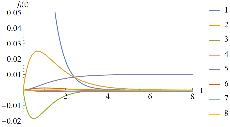
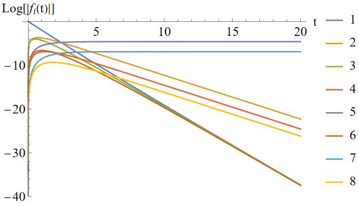
In figure 1, we plot the correlation pattern coefficient as a function of time. We see that some transient correlation patterns that connect the left-boundary condition and right-boundary condition may appear at intermediate times. However, they eventually die out at long real-time, leaving only and :
| (17) |
This means that equals the prediction of the Haar ensemble enwiki:1183923474 ; Collins_2022 ; Gu2013MomentsOR ; zhang2015matrix ; Czech:2023rbh . In section 3.1, we will show that equals the Haar’s prediction for arbitrary .
2.2 One-replica observables
Spectral Form Factor.
The spectral form factor (SFF) is given by:
| (18) |
which smoothly interpolates between the identity and Haar ensemble. We see that at the timescale , the two terms become comparable, and SFF is of order one.
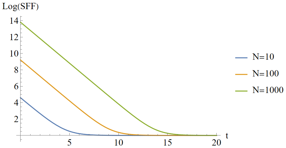
Similar to the Brownian SYK, SFF in BGUE monotonically decreases with time, and there is no linear ramp as in the static GUE or static SYK model Cotler2017BHandRMT . In figure 2, we plot SFF with respect to time.
Two-point function.
Consider the following two-point function:
| (19) |
which smoothly interpolates between and . This indicates that the correlation connecting the left and right of the contour gradually dies out at the timescale .
It is helpful to compare this with the result of BDSSYK (Brownian Double-Scaled-SYK), whose two-point function has the form of Milekhin:2023bjv ; Stanford:2023npy . There are several immediate remarks:
-
1.
Emergence of tomperature in BGUE. The emergence of a timescale in infinite temperature (Brownian has no energy conservation) is like tomperature SusskindLin2022nss .
-
2.
Replica-wormhole in BGUE. There is no replica wormhole in BDSSYK. This is because we already take the infinite dimension limit, and all higher topological changes are suppressed. In our BGUE model, the non-decaying part of the two-point function Stanford:2020wkf ; Saad:2019pqd ; JuanMaldacena_2003 is reminiscent of the replica wormhole Penington2022 ; Almheiri2020 .
-
3.
Dependence on matter scaling dimension. In BDSSYK, the scaling dimension of matter chords, , appears in the exponent, which affects the timescale explicitly. In BGUE, the matter operators only appear as the boundary condition, and the damping mode only depends on . BGUE is recovered as a special limit in BDSSYK by taking the -parameter to zero.
2.3 Two-replica observables
Fluctuation of spectral form factor.
| (20) | ||||
We notice that , which is reasonable, and . We can also fix and scale to infinity:
| (21) |
Therefore, the maximal value of variance is of order , and the timescale for reaching this maximal fluctuation is of order one.
A more physical way of quantifying the size of the fluctuation is to calculate the relative variance: , which is shown in figure 3. We see that for , , and for , . This is consistent with the case in GUE or SYK, where the fluctuation in the plateau regime is large compared to the dip regime Cotler2017BHandRMT .

Fluctuation of two-point functions.
In general, the expression for the fluctuation of the two-point function is complicated, as calculating involves many contour pairings, where each of the terms will contribute respectively as: , , , , , , , . To simplify the expression, we consider three cases:
-
1.
Case 1: , where we imagine are Pauli operators on different spatial sites. In this case, we have , meaning the average two-point function vanishes.
-
2.
Case 2: , where we imagine are Pauli operators on the same spatial site, but with different flavors. In this case, we have , meaning the average two-point function vanishes.
-
3.
Case 3: , where we consider the auto-correlation of a Pauli operator. In this case, we have .
The variance of these three types of correlation functions is given by:
| (22) | ||||
We notice that the variance is of order one at arbitrary . This finite variance is non-trivial for and , since their average values vanish. This non-zero variance with zero mean is due to the effect of the replica wormhole, as indicated in Stanford:2020wkf .
These three fluctuations are shown in figure 4, where we see that at intermediate times, the behavior of fluctuation depends on whether commute or anti-commute, and also on whether are the same or not. This originates from terms like , whose coefficients are non-zero only at intermediate times.
We also notice that the initial growth of variance differs in the three cases. To see this, we may work out the Taylor expansion at short times:
| (23) | ||||
It is interesting to see that for , the variance grows linearly while the others grow quadratically. It is also interesting to observe that the first two coefficients are independent of .
We can also work out the limit where goes to infinity while keeping fixed, where the variance is of order one:
| (24) | ||||
Out-of-Time-Ordered Correlator (OTOC)
Assuming , the relation between (anti)commutator-squared and OTOC is given by:
| (25) |
where we choose (anti)commutator and (plus)minus sign on RHS if at the initial time (anti)commute with each other. The commutator of three cases is given by:
| (26) | ||||
We may take while keeping finite:
| (27) | ||||
We note that OTOC and commutators still have non-trivial dynamics in the infinite limit. This hyper-fast scrambling behavior Susskind2021omt ; Susskind2021dfc ; Susskind2021esx ; Susskind2022fop ; Susskind2022dfz ; SusskindLin2022nss ; Susskind2022bia ; Susskind2023hnj ; Susskind2023rxm is consistent with other Brownian models such as BDSSYK Milekhin:2023bjv ; Stanford:2023npy . This is opposed to static SYK, where the timescale for scrambling is Maldecena2016 , meaning no scrambling dynamics will occur at infinite . The behavior of commutators is shown in figure 4.
Second Rényi Entropy
Consider we evolve the system from a pure product state. At time , we consider the sub-system with Hilbert space dimension . The second Rényi entropy (actually we first average over the purity, and then take the log) is given by:
| (28) |
We see that the system approaches the Page curve of the Haar random ensemble at order one time, consistent with studies in the scrambling phase of MIPT in (0+1)-dimensional models koh2022experimental ; li2022cross ; MIPT1 ; MIPT10 ; MIPT2 ; MIPT24 ; MIPT3 ; MIPT30 ; MIPT5 ; MIPT7 ; noel2022measurement .
We can also study the velocity of entropy growth at the initial time:
| (29) |
We see that the coefficient of approaches for arbitrary in the infinite limit, and the coefficient of vanishes in the infinite limit. This shows that in the infinite limit, the linear-in-time growth rate of entropy for all subsystems is the same:
| (30) |
Frame potential for unitary two-design
Given any ensemble of unitary matrices, the frame potential Scott_2008 ; Gross_2007 ; hunterjones2019unitary ; PRXQuantum.2.030316 ; Jian:2022pvj ; Cotler2017ChaosComplexityRMT ; Roberts2017ChaosByDesign , relevant to -designs, is defined as:
| (31) |
where and are drawn independently from the same ensemble .
Frame potential naturally measures whether is ’dispersed’ or ’concentrated’. Consider an extreme case where the ensemble consists of only one element with probability one. In this case, the forward evolution perfectly cancels the backward evolution, leading to , which results in the maximal possible value of the frame potential. On the other hand, if is dispersed, then two independently drawn samples and are likely to be very different, meaning that will be very small. The most ’dispersed’ ensemble is the Haar ensemble, indicating that is the smallest among all .
In our case, we can calculate , which is relevant for comparing 2-designs. For the identity ensemble (an ensemble whose single element is the identity matrix), and for the Haar random ensemble we have .
The formula for the frame potential of BGUE is , which is the square of the average spectral form factor. The explicit formula is given by:
| (32) | ||||
which smoothly interpolate between and . In section 3.2, we obtain the frame potential for arbitrary up to the second excited states of . For , the second excited states are already the highest energy states.
3 Approaching -design for arbitrarily many replicas
In this section, we are interested in how approaches the Haar ensemble’s prediction for large but finite . Therefore, in section 3.1, we focus on the low-energy spectrum (up to the family of second excited states) of , which governs the long-time behavior of . Using this spectral information, in section 3.2, we calculate the frame potential and estimate a lower bound on the time needed to approach an -approximated -design.
Recall there are -replicas with forward-moving contours labeled by and backward-moving contours labeled by . The Hilbert space is . The averaged evolution operator is defined by:
| (33) |
The Lindbladian is given by:
| (34) | ||||
3.1 Low energy spectrum
3.1.1 Ground states
In this section, we show that the ground state energy of is zero, with degeneracy . The ground state manifold is spanned by permutation matrix elements. The projector onto the ground state manifold equals the prediction of the Haar average, indicating that approaches the Haar ensemble as .
To be precise, the ground state of is labeled by a permutation element :
| (35) |
where is the basis label on the individual Hilbert space of each contour. A diagrammatic example for is:
| (36) |
In these diagrams, the -contours are arranged from up to down in the order of (see the label in (36) for example). Notice that in section 2, the diagram for equation (11) for , the contour is ordered as from up to down.
Now, we are ready to show that is indeed the eigenstate of with zero energy. Let’s act on . One kind of term coming from is:
| (37) |
Here, to simplify the diagram like (36), we use black lines to indicate the links that are relevant for calculation, and a gray background to represent the other links that are not involved in this step of the calculation.
| Label | Equation | # |
|---|---|---|
The number of such terms is . So, this contribution cancels the constant part in . The other terms in look like:
| (38) |
They are canceled by the action of and :
| (39) |
We notice that the number of terms matches. Putting everything together, this shows that .
We notice that the set of ground states are not orthogonal. In fact, if we define their Gram matrix as ( counts the number of cycles in permutation element ) and denote its (pseudo)inverse matrix as ( is exactly the Weingarten function enwiki:1183923474 ; Collins_2022 ; Gu2013MomentsOR ; zhang2015matrix ; Czech:2023rbh ), then the ground state manifold projector is given by:
| (40) |
This shows that BGUE evolves and saturates to the Haar ensemble at .
3.1.2 First excited states
In this section, we explicitly construct the wavefunction of the first excited states and show that their energy is with degeneracy .
The first excited states are built upon some modifications of the ground state, where one of the links is broken, and two computational basis indices are glued onto the two broken ends. An example for is:
| (41) |
where label the position of the broken links. Let’s act on , and the five kinds of terms (labeled as ) are recorded in table 1.
Next, we act on , and the four kinds of terms (labeled as ) are recorded in table 2.
| Label | Equation | # |
|---|---|---|
We notice that cancels , cancels , and cancels . Therefore, the surviving terms are and .
Grouping everything together, we obtain:
| (42) | ||||
Notice that belongs to the ground state manifold. Therefore, we may consider a linear superposition to get rid of this term. Define to be an coefficient matrix:
| (43) |
Then we have:
| (44) |
We see that by choosing to be traceless, namely , we obtain that . So we successfully construct the first excited states with eigenvalue .
Next, we aim to determine the degeneracy of the first excited states. There are choices for the traceless matrix , choices for the positions of located at , and choices for . Therefore, we may conclude that the degeneracy is .
We need to show that they are linearly independent. To do so, we analyze the inner product in the large limit. We first notice that when or , the inner product is at most . But for and , the inner product is of order . This shows the Gram matrix is almost block diagonal in the infinite limit. So, the states with or persist to be linearly independent in large but finite by continuity. Next, we consider the inner product within each block:
| (45) |
This is a standard inner product for traceless matrices. So, there are indeed linearly independent choices of .
In summary, this shows that the degeneracy is indeed at large but finite . We expect that some null states will appear if is of order , which reduces degeneracy. This also happens in the ground state manifold, whose degeneracy starts to decrease from when saad2019semiclassical .
3.1.3 Second excited states
In this section, we study the family of second excited states of . The energy spectrum splits into , and their corresponding degeneracy is summarized in table 4.
Similarly, the second excited states are constructed by breaking two links of ground states. An example for is given by:
| (46) |
where label the position of broken links.
Let’s act on . From the experience in ground states and first excited states, we see that the following two kinds of terms in will cancel those in : (1) exchange the ends of two unbroken links; (2) exchange the ends of one unbroken link and one broken link. So, the terms that are not canceled are the following four kinds of terms (labeled as ) recorded in table 3.
| Label | Comes from where? | Equation | # |
|---|---|---|---|
Putting everything together, we obtain:
| (47) | ||||
The four terms on the second and third lines correspond to in table 3. From the diagrams, these states have only one broken link, which belongs to the manifold of the first excited states. To construct eigenstates, we need these four terms to vanish. To achieve this, we define a four-leg tensor and define the linear superposition state:
| (48) |
Eliminating four terms from is equivalent to imposing the following four linear constraints on :
| (49) |
Then, the equation is reduced to:
| (50) | ||||
To make eigenstates, we need to further require that is symmetric/anti-symmetric in its first two indices and symmetric/anti-symmetric in its last two indices. So, we obtain:
| (51) |
Next, we need to count the degeneracy. Similar to the case of the first excited states, the inner product with different positions or different is at most of order . Those states with the same position and permutation element have an inner product of order . Therefore, states with different positions or different permutations are linearly independent in large but finite . So, counting the position and permutation gives degeneracy .
Then, we need to count the degeneracy of , satisfying symmetry conditions and four linear constraints. Notice that under such symmetry of indices, four constraints are satisfied if and only if any one of them is satisfied. We choose as a representative. Since:
| (52) |
where we define to be a state on an auxiliary Hilbert space that leaves the position and permutation fixed and implicit.
Our strategy to construct the wave function under symmetry and constraint is to start with an arbitrary , and then construct the projector that projects onto the subspace respecting symmetry and constraint. Then is what we want. The number of linearly independent basis of equals the rank of projector , namely .
Before constructing projectors corresponding to four symmetry conditions in equation (51), we fix some notation on the auxiliary Hilbert space. The states are diagrammatically represented by:
| (53) |
Define three kinds of projectors and a special state :
| (54) |
where is a symmetric projector and is an anti-symmetric projector. Then, are given by:
| (55) | ||||
One can check that satisfies the symmetry condition and constraint corresponding to . Also, one can check that , which is indeed a properly orthonormalized projector. Picking up factor from the degeneracy of position and permutation, then by evaluating , we can obtain the full degeneracy, which we summarize in table 4.
| Eigenvalue of | Degeneracy |
|---|---|
3.1.4 General excited states in the infinite limit
For general highly excited states, it is challenging to exactly solve the wave function, energy, and degeneracy. However, in the infinite limit, things simplify.
Consider the excited states (), whose wave function is similarly constructed by breaking -links on top of ground states, and then gluing computational basis to broken ends. These states are labeled by . Action of on it will generate four kinds of terms analogous to in table 3. In the infinite limit, are suppressed by while are not. Therefore, :
| (56) | ||||
So, they are eigenstates with energy . The degeneracy of these states is counted to be .
3.2 Approaching -design
Given an ensemble of unitaries acting on Hilbert space with dimension , we can ask how close is to the Haar ensemble. The distance between two ensembles can be measured by comparing their moments. Let be an operator on -copies of Hilbert space: . Then define the following moment map channel Jian:2022pvj :
| (57) |
Then we say that is an -approximated -design if the distance between two channels is smaller than measured in the diamond norm Jian:2022pvj :
| (58) |
Since the diamond norm is usually hard to calculate, we may use the frame potential:
| (59) |
to bound the diamond norm via the following inequality Jian:2022pvj :
| (60) |
The frame potential for the Haar ensemble is given by . In our BGUE case, we find that:
| (61) | ||||
where we use the fact that and . We see that the frame potential only depends on the spectrum and degeneracy of . Therefore, using the results of ground states, first excited states, and second excited states, we can approximate the frame potential in the long-time limit:
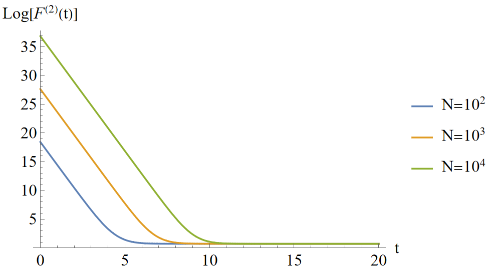
| (62) | ||||
Neglecting second excited states, we obtain the time for BGUE to approach an -approximated -design is:
| (63) |
The linear-in- scaling is consistent with the Brownian SYK result Jian:2022pvj .
One can also use the result in section 3.1.4 to calculate the frame potential in a certain limit: scaling while keeping finite:
| (64) |
Using Laguerre polynomial , we obtain that:
| (65) |
4 Application in classical shadow tomography
4.1 Brief review of classical shadow tomography
The method of classical shadow tomography aims to predict many observables from just a few measurements. The central spirit of this method is: First do measurement, and then ask questions Huang2020 ; Elben2023 ; PhysRevLett.127.030503 ; PhysRevLett.126.190505 .
An illuminating example is: given an unknown single qubit state , we want to predict the expectation values of all three Pauli observables up to error by performing as few measurements as possible. The observation is that since do not commute, we cannot measure them simultaneously. In other words, if we measure to high precision with an error smaller than (e.g., we perform measurements in the -eigenbasis), then the error of predicting would be much larger than . Therefore, instead of measuring in the eigenbasis of many times, we measure in some random directions a few times, so that each measurement can moderately predict all three .
Now, we are ready to formulate the task and method of classical shadow tomography Huang2020 . Consider we are handed an experimental oracle that can produce an unknown state on an -qubit Hilbert space. We want to perform some measurements on , and then predict the expectation value of a set of -observables . The idea is similar: we perform some random measurements on . This is achieved by applying a random unitary ( is a pre-designed ensemble of unitaries) on , and then perform measurements on the computational basis, with the measurement result being . We perform such procedures for times, each time recording a pair .
Define to be the measurement channel:
| (66) |
For a tomographically complete channel Huang2020 , is invertible. Therefore, we obtain:
| (67) |
In practice, we obtain realizations of , therefore an unbiased estimation of is by replacing by a finite sum:
| (68) |
Then we can use to calculate , which is an unbiased estimator of :
| (69) |
The performance or accuracy of is related to the variance of the classical random variable , which is bounded by:
| (70) |
Since one wants to define a quantity that quantifies the variance for generic , which only depends on , not , we can further maximize over or take an average over . Finally, we obtain a max-version or a mean-version of the shadow norm:
| max-version: | (71) | |||
| mean-version: |
We notice that the measurement channel and therefore the shadow norm depends on the choice of random unitary ensemble . Therefore, for a given type of interested , we need to design to make the shadow norm as small as possible, which in turn decreases the number of measurements needed Huang2020 . For example, if is a Pauli string with length , and is an ensemble of shallow circuits with depth (one can imagine that for instance every is a brick-wall circuit with depth-, with every local 2-qubit-gate being Haar-random), then there exists an optimal depth that minimizes the shadow norm PhysRevLett.130.230403 ; PhysRevResearch.5.023027 . See PRXQuantum.5.020304 ; PhysRevLett.130.230403 ; PhysRevResearch.4.013054 ; PhysRevResearch.5.023027 ; Akhtar2023scalableflexible ; PhysRevB.109.094209 ; akhtar2024dualunitary for more schemes of designing and chen2021hierarchy ; 9719827 ; Aharonov2022 for information-theoretical upper/lower bounds that assess the performance of the shadow tomography method.
4.2 Classical shadow tomography using BGUE
In this section, we apply BGUE to the task of classical shadow tomography Huang2020 . We derive explicit analytical results on shadow norm as a function of . We observe that an optimal time exists as a function of the off-diagonal portion of , which minimizes the shadow norm. This phenomenon is analogous to the optimal circuit depth in the shallow-circuit protocol PhysRevLett.130.230403 ; PhysRevResearch.5.023027 .
Let’s start by calculating the measurement channel. The measurement channel acting on the density matrix is defined as:
| (72) |
This can be evaluated exactly using our two-replica result in section 2, using the diagrams in equation (11). The result is given by:
| (73) |
where is the off-diagonal part of and is the traceless diagonal part of . The coefficients are given by:
| (74) | ||||
where is defined in equation (16). The inverse channel can be readily calculated:
| (75) |
Shadow Norm.
Similarly, are the off-diagonal and traceless diagonal part of , respectively. Next, we calculate the (mean-version) shadow norm for a traceless Hermitian operator :
| (76) | ||||
where we used the fact that . Notice that . So, we may define to be the portion of the off-diagonal part and traceless diagonal part inside : , , with the constraint . Thus, the shadow norm in units of the two-norm is given by:
| (77) |
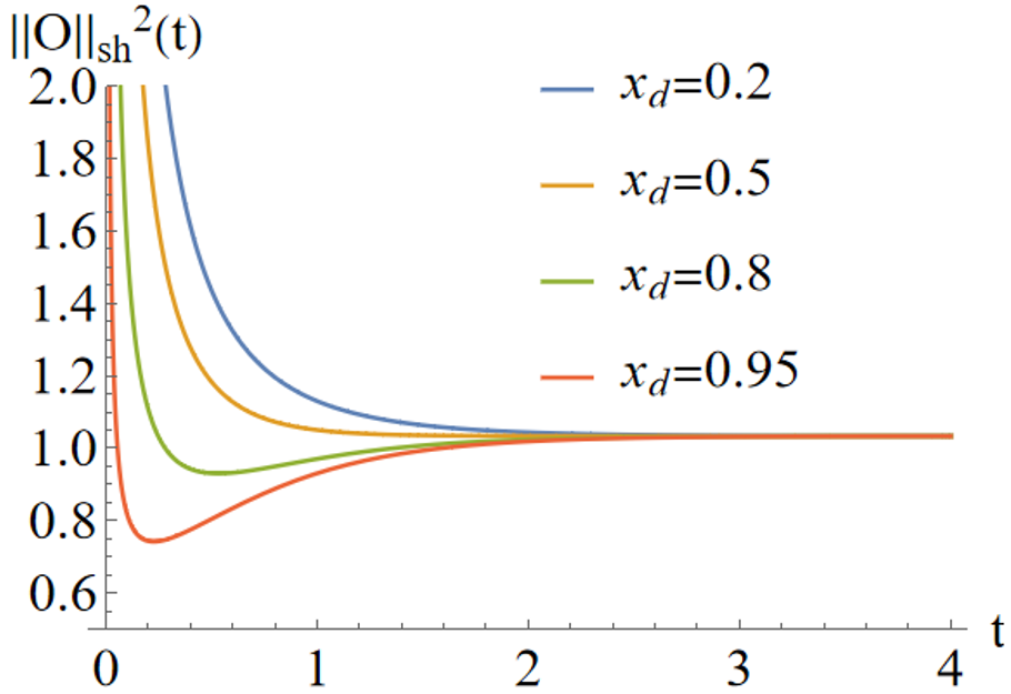
We first analyze the shadow norm of a purely diagonal () or purely off-diagonal operator (). We see that increases with time. This means that the scrambling will decrease the efficiency of predicting the diagonal operator. On the other hand, decreases with time. This means that the scrambling will improve the efficiency of predicting the off-diagonal operator. We notice that , which means in the initial time, we cannot predict the off-diagonal operator at all. This is reasonable since without we are just measuring the computational basis, which only knows about the diagonal entries of the operator. We also notice that as , , approaching the global Haar random result Huang2020 . This is reasonable since Haar randomness is basis independent; therefore, diagonal and off-diagonal should have the same shadow norm. A plot of these phenomena can be found in figure 6.
Optimal Time.
Now, we consider has both and components. It turns out that when , there is an optimal time such that is minimal:
| (78) |
The minimal shadow norm is given by:
| (79) |
This phenomenon is observed in numerical simulations in figure 6. The existence of an optimal time as a function of the off-diagonal portion is analogous to the optimal circuit depth as a function of the Pauli-string’s length in shallow-circuit classical shadow tomography PhysRevLett.130.230403 ; PhysRevResearch.5.023027 .
5 Conclusion
In this study, we have constructed and thoroughly analyzed the Brownian generalization of the Gaussian Unitary Ensemble (BGUE). Our investigation encompassed both the non-equilibrium dynamics, complexity and test of applications in classical shadow tomography, yielding significant insights into its behavior and potential applications in broaden quantum information tasks.
We began the study of non-equilibrium dynamics in BGUE by deriving explicit analytical expressions for various one-replica and two-replica variables at finite and . These variables include the spectral form factor, its fluctuation, the two-point function, the fluctuations of the two-point function, out-of-time-order correlators (OTOC), the second Rényi entropy, and the frame potential for unitary 2-designs.
Our results revealed that BGUE exhibits hyperfast scrambling and the emergence of tomperature. Additionally, we identified replica-wormhole-like contributions, leading to a non-decaying two-point function as and non-vanishing fluctuations of the two-point function with zero mean value.
We further explored the complexity of BGUE, determining the time required for the ensemble to approximate the Haar ensemble in terms of -design. Our findings indicate that the timescale is linear in , consistent with previous studies on the Brownian Sachdev-Ye-Kitaev (SYK) model. In our investigation of the low-energy eigen-wavefunctions, spectrum, and degeneracy of the effective imaginary-time evolution operator on -replicated contours, we derived long-time results for the frame potential, confirming that the time required for BGUE to reach -design is linear in .
In the final section, we applied the BGUE model to classical shadow tomography. We derived analytical results for the shadow norm and identified an optimal time that minimizes the shadow norm, analogous to the optimal circuit depth in shallow-circuit shadow tomography.
There are some possible interesting questions based on our study of BGUE:
-
1.
Exact for three-replica observables. Many interesting observables need three replicas. One relevant example is the max-version shadow norm defined in (71).
-
2.
Application in other quantum information tasks. For example, we can study the quantum causal influence (QCI) Cotler_2019QCI , spacetime entanglement entropy in super-density operator formalism Cotler_2018Superdensity , and channel capacity Hosur_2016 . We are currently exploring these directions.
-
3.
Adding noise and measurement. We can add decoherence and measurement to the scrambling of BGUE, which can be used to study Measurement Induced Phase Transition or Noise Induced Phase Transition extensively studied in recent literature.
-
4.
Brownian generalization of other ensemble. One direct generalization is consider different symmetry class, like Brownian Gaussian Orthogonal Ensemble (BGOE) and Brownian Sympletic Ensemble (BGSE).
In conclusion, our study provides a comprehensive understanding of the non-equilibrium dynamics and complexity of BGUE, demonstrating its scrambling behavior and potential for its applications in quantum information tasks such as classical shadow tomography. The analytical techniques and results presented here lay a foundation for future explorations of Brownian random matrix models and their applications in quantum physics and beyond.
Acknowledgements.
I would like to thank Wanda Hou, Xiao-Liang Qi, Douglas Stanford, Hong-Yi Wang, Jinzhao Wang, Jiuci Xu, Shunyu Yao, Yi-Zhuang You, and Yuzhen Zhang for helpful discussion. I would especially thank Yuzhen Zhang for stimulating conversations on frame potential. I would also thank numerous useful discussions with Hong-Yi Wang on classical shadow tomography. I thank professor Xiao-Liang Qi’s support by National Science Foundation under grant No.2111998 and the Simons Foundation.Appendix A Subset of High Energy Spectrum
In this appendix, we aim to gain a deeper understanding of the generic high-energy spectrum of . Although deriving the general formula for the spectrum and degeneracy by breaking more links on ground states is challenging, we demonstrate a special case where is a subset of the spectrum of , using a different method. To achieve this, we work in an operator basis instead of a state basis.
Consider as an operator on the Hilbert space . is defined by the equal-weight summation of all diagrams with: (1) -lines connecting upper left and upper right; (2) -lines connecting lower left and lower right; (3) -lines connecting upper left and lower left; and (4) -lines connecting upper right and lower right. The number of terms in the summand of is:
| (80) |
| Label | Source | Equation | Count | Mapping of diagrams |
|---|---|---|---|---|
An example of a diagram within the summand of would be:
| (81) |
Another example relates to the calculation of the 2-replica case in the previous section 2: , , and , where is defined in equation (11).
Using equation (12), we find that , , and . We see that the action of is closed in these three bases, which means the vector space defined by forms a three-dimensional representation of .
Motivated by this special result at , in this appendix, we show that the linear space forms a -dimensional representation of . We further show that the representation matrix of is upper-triangular. Therefore, we can determine the eigenvalues from the diagonal entries of the representation matrix, which turn out to be .
Let’s act on . The analysis is similar to that in the second excited states, retaining the four terms recorded in table 5.
Therefore, we see that the action of can either map diagrams in to diagrams in (process ), or map diagrams in to diagrams in (processes ). By the permutation symmetry of and , we conclude that takes to be a linear superposition of and :
| (82) | ||||
This shows that the representation matrix of is upper-triangular, and therefore we can determine the eigenvalues from the diagonal entries, as claimed at the beginning of this appendix. We also note that when taking , these equations successfully reproduce the two-replica results.
References
- (1) C.-F. Chen, J. Docter, M. Xu, A. Bouland and P. Hayden, Efficient Unitary T-designs from Random Sums, 2402.09335.
- (2) M. Mehta, Random Matrices, ISSN, Elsevier Science (2004).
- (3) J. Cotler, N. Hunter-Jones, J. Liu and B. Yoshida, Chaos, complexity, and random matrices, Journal of High Energy Physics 2017 (2017) 48.
- (4) D.A. Roberts and B. Yoshida, Chaos and complexity by design, Journal of High Energy Physics 2017 (2017) 121.
- (5) C.-F. Chen, A. Bouland, F.G.S.L. Brandão, J. Docter, P. Hayden and M. Xu, Efficient unitary designs and pseudorandom unitaries from permutations, 2404.16751.
- (6) H. Lin and L. Susskind, Infinite Temperature’s Not So Hot, 2206.01083.
- (7) P. Saad, Late Time Correlation Functions, Baby Universes, and ETH in JT Gravity, 1910.10311.
- (8) J. Maldacena, Eternal black holes in anti-de sitter, Journal of High Energy Physics 2003 (2003) 021.
- (9) D. Stanford, More quantum noise from wormholes, 2008.08570.
- (10) C. Dankert, Efficient simulation of random quantum states and operators, quant-ph/0512217.
- (11) C. Dankert, R. Cleve, J. Emerson and E. Livine, Exact and approximate unitary 2-designs and their application to fidelity estimation, Phys. Rev. A 80 (2009) 012304.
- (12) D. Gross, K. Audenaert and J. Eisert, Evenly distributed unitaries: On the structure of unitary designs, Journal of Mathematical Physics 48 (2007) .
- (13) A. Ambainis and J. Emerson, Quantum t-designs: t-wise independence in the quantum world, .
- (14) S. Sachdev, Bekenstein-hawking entropy and strange metals, Phys. Rev. X 5 (2015) 041025.
- (15) J. Maldacena and D. Stanford, Remarks on the sachdev-ye-kitaev model, Phys. Rev. D 94 (2016) 106002.
- (16) S.-K. Jian, G. Bentsen and B. Swingle, Linear growth of circuit complexity from Brownian dynamics, JHEP 08 (2023) 190 [2206.14205].
- (17) H.-Y. Huang, R. Kueng and J. Preskill, Predicting many properties of a quantum system from very few measurements, Nature Physics 16 (2020) 1050.
- (18) M. Ippoliti, Y. Li, T. Rakovszky and V. Khemani, Operator relaxation and the optimal depth of classical shadows, Phys. Rev. Lett. 130 (2023) 230403.
- (19) H.-Y. Hu, S. Choi and Y.-Z. You, Classical shadow tomography with locally scrambled quantum dynamics, Phys. Rev. Res. 5 (2023) 023027.
- (20) S. Guo, M. Sasieta and B. Swingle, Complexity is not Enough for Randomness, 2405.17546.
- (21) J.S. Cotler, G. Gur-Ari, M. Hanada, J. Polchinski, P. Saad, S.H. Shenker et al., Black holes and random matrices, Journal of High Energy Physics 2017 (2017) 118.
- (22) J. Maldacena, S.H. Shenker and D. Stanford, A bound on chaos, Journal of High Energy Physics 2016 (2016) 106.
- (23) Y. Sekino and L. Susskind, Fast scramblers, Journal of High Energy Physics 2008 (2008) 065.
- (24) D.A. Roberts, D. Stanford and A. Streicher, Operator growth in the syk model, Journal of High Energy Physics 2018 (2018) 122.
- (25) X.-L. Qi and A. Streicher, Quantum epidemiology: operator growth, thermal effects, and syk, Journal of High Energy Physics 2019 (2019) 12.
- (26) A. Lucas, Operator size at finite temperature and planckian bounds on quantum dynamics, Phys. Rev. Lett. 122 (2019) 216601.
- (27) A. Nahum, J. Ruhman, S. Vijay and J. Haah, Quantum entanglement growth under random unitary dynamics, Phys. Rev. X 7 (2017) 031016.
- (28) A. Nahum, S. Vijay and J. Haah, Operator spreading in random unitary circuits, Phys. Rev. X 8 (2018) 021014.
- (29) C.W. von Keyserlingk, T. Rakovszky, F. Pollmann and S.L. Sondhi, Operator hydrodynamics, otocs, and entanglement growth in systems without conservation laws, Phys. Rev. X 8 (2018) 021013.
- (30) P. Hayden, S. Nezami, X.-L. Qi, N. Thomas, M. Walter and Z. Yang, Holographic duality from random tensor networks, Journal of High Energy Physics 2016 (2016) 9.
- (31) T. Zhou and A. Nahum, Entanglement membrane in chaotic many-body systems, Phys. Rev. X 10 (2020) 031066.
- (32) M.P.A. Fisher, V. Khemani, A. Nahum and S. Vijay, Random quantum circuits, 2022. 10.48550/ARXIV.2207.14280.
- (33) J.M. Koh, S.-N. Sun, M. Motta and A.J. Minnich, Experimental realization of a measurement-induced entanglement phase transition on a superconducting quantum processor, 2022.
- (34) Y. Li, Y. Zou, P. Glorioso, E. Altman and M.P.A. Fisher, Cross entropy benchmark for measurement-induced phase transitions, 2022. 10.48550/ARXIV.2209.00609.
- (35) B. Skinner, J. Ruhman and A. Nahum, Measurement-induced phase transitions in the dynamics of entanglement, Phys. Rev. X 9 (2019) 031009.
- (36) M.J. Gullans and D.A. Huse, Dynamical purification phase transition induced by quantum measurements, Phys. Rev. X 10 (2020) 041020.
- (37) Y. Li, X. Chen and M.P.A. Fisher, Quantum zeno effect and the many-body entanglement transition, Phys. Rev. B 98 (2018) 205136.
- (38) S.-K. Jian, C. Liu, X. Chen, B. Swingle and P. Zhang, Measurement-induced phase transition in the monitored sachdev-ye-kitaev model, Phys. Rev. Lett. 127 (2021) 140601.
- (39) C.-M. Jian, Y.-Z. You, R. Vasseur and A.W.W. Ludwig, Measurement-induced criticality in random quantum circuits, Phys. Rev. B 101 (2020) 104302.
- (40) X. Yu and X.-L. Qi, Measurement-induced entanglement phase transition in random bilocal circuits, 2022. 10.48550/ARXIV.2201.12704.
- (41) Y. Li and M.P.A. Fisher, Statistical mechanics of quantum error correcting codes, Phys. Rev. B 103 (2021) 104306.
- (42) Y. Li, X. Chen and M.P.A. Fisher, Measurement-driven entanglement transition in hybrid quantum circuits, Phys. Rev. B 100 (2019) 134306.
- (43) C. Noel, P. Niroula, D. Zhu, A. Risinger, L. Egan, D. Biswas et al., Measurement-induced quantum phases realized in a trapped-ion quantum computer, Nature Physics 18 (2022) 760.
- (44) A. Milekhin and J. Xu, Revisiting Brownian SYK and its possible relations to de Sitter, 2312.03623.
- (45) D. Stanford, S. Vardhan and S. Yao, Scramblon loops, 2311.12121.
- (46) D. Stanford, Z. Yang and S. Yao, Subleading weingartens, Journal of High Energy Physics 2022 (2022) 200.
- (47) Wikipedia contributors, Partition algebra — Wikipedia, the free encyclopedia, 2023.
- (48) D.E. Parker, X. Cao, A. Avdoshkin, T. Scaffidi and E. Altman, A universal operator growth hypothesis, Phys. Rev. X 9 (2019) 041017.
- (49) A. Bhattacharyya, S.S. Haque, G. Jafari, J. Murugan and D. Rapotu, Krylov complexity and spectral form factor for noisy random matrix models, Journal of High Energy Physics 2023 (2023) 157.
- (50) J. Erdmenger, S.-K. Jian and Z.-Y. Xian, Universal chaotic dynamics from krylov space, Journal of High Energy Physics 2023 (2023) .
- (51) A. Kar, L. Lamprou, M. Rozali and J. Sully, Random matrix theory for complexity growth and black hole interiors, Journal of High Energy Physics 2022 (2022) 16.
- (52) C. Liu, H. Tang and H. Zhai, Krylov complexity in open quantum systems, Phys. Rev. Res. 5 (2023) 033085.
- (53) H. Tang, Operator Krylov complexity in random matrix theory, 2312.17416.
- (54) H. Tang, Entanglement entropy in type II1 von Neumann algebra: examples in Double-Scaled SYK, 2404.02449.
- (55) P. Nandy, A.S. Matsoukas-Roubeas, P. Martínez-Azcona, A. Dymarsky and A. del Campo, Quantum Dynamics in Krylov Space: Methods and Applications, 2405.09628.
- (56) Wikipedia contributors, Weingarten function — Wikipedia, the free encyclopedia, 2023.
- (57) B. Collins, S. Matsumoto and J. Novak, The weingarten calculus, Notices of the American Mathematical Society 69 (2022) 1.
- (58) Y. Gu, Moments of random matrices and weingarten functions by yinzheng gu, 2013, https://api.semanticscholar.org/CorpusID:202611603.
- (59) L. Zhang, Matrix integrals over unitary groups: An application of schur-weyl duality, 2015.
- (60) B. Czech, S. Shuai and H. Tang, Entropies and reflected entropies in the Hayden-Preskill protocol, JHEP 02 (2024) 040 [2310.16988].
- (61) G. Penington, S.H. Shenker, D. Stanford and Z. Yang, Replica wormholes and the black hole interior, Journal of High Energy Physics 2022 (2022) 205.
- (62) A. Almheiri, T. Hartman, J. Maldacena, E. Shaghoulian and A. Tajdini, Replica wormholes and the entropy of hawking radiation, Journal of High Energy Physics 2020 (2020) 13.
- (63) L. Susskind, De Sitter Holography: Fluctuations, Anomalous Symmetry, and Wormholes, Universe 7 (2021) 464 [2106.03964].
- (64) L. Susskind, Black Holes Hint Towards De Sitter-Matrix Theory, 2109.01322.
- (65) L. Susskind, Entanglement and Chaos in De Sitter Space Holography: An SYK Example, JHAP 1 (2021) 1 [2109.14104].
- (66) E. Shaghoulian and L. Susskind, Entanglement in De Sitter space, JHEP 08 (2022) 198 [2201.03603].
- (67) L. Susskind, Scrambling in Double-Scaled SYK and De Sitter Space, 2205.00315.
- (68) L. Susskind, De Sitter Space, Double-Scaled SYK, and the Separation of Scales in the Semiclassical Limit, 2209.09999.
- (69) L. Susskind, De Sitter Space has no Chords. Almost Everything is Confined, 2303.00792.
- (70) L. Susskind, A Paradox and its Resolution Illustrate Principles of de Sitter Holography, 2304.00589.
- (71) A.J. Scott, Optimizing quantum process tomography with unitary2-designs, Journal of Physics A: Mathematical and Theoretical 41 (2008) 055308.
- (72) N. Hunter-Jones, Unitary designs from statistical mechanics in random quantum circuits, 2019.
- (73) F.G. Brandão, W. Chemissany, N. Hunter-Jones, R. Kueng and J. Preskill, Models of quantum complexity growth, PRX Quantum 2 (2021) 030316.
- (74) P. Saad, S.H. Shenker and D. Stanford, A semiclassical ramp in syk and in gravity, 2019.
- (75) A. Elben, S.T. Flammia, H.-Y. Huang, R. Kueng, J. Preskill, B. Vermersch et al., The randomized measurement toolbox, Nature Reviews Physics 5 (2023) 9.
- (76) H.-Y. Huang, R. Kueng and J. Preskill, Efficient estimation of pauli observables by derandomization, Phys. Rev. Lett. 127 (2021) 030503.
- (77) H.-Y. Huang, R. Kueng and J. Preskill, Information-theoretic bounds on quantum advantage in machine learning, Phys. Rev. Lett. 126 (2021) 190505.
- (78) M. Ippoliti and V. Khemani, Learnability transitions in monitored quantum dynamics via eavesdropper’s classical shadows, PRX Quantum 5 (2024) 020304.
- (79) H.-Y. Hu and Y.-Z. You, Hamiltonian-driven shadow tomography of quantum states, Phys. Rev. Res. 4 (2022) 013054.
- (80) A.A. Akhtar, H.-Y. Hu and Y.-Z. You, Scalable and Flexible Classical Shadow Tomography with Tensor Networks, Quantum 7 (2023) 1026.
- (81) A.A. Akhtar, H.-Y. Hu and Y.-Z. You, Measurement-induced criticality is tomographically optimal, Phys. Rev. B 109 (2024) 094209.
- (82) A.A. Akhtar, N. Anand, J. Marshall and Y.-Z. You, Dual-unitary classical shadow tomography, 2024.
- (83) S. Chen, J. Cotler, H.-Y. Huang and J. Li, A hierarchy for replica quantum advantage, 2021.
- (84) S. Chen, J. Cotler, H.-Y. Huang and J. Li, Exponential separations between learning with and without quantum memory, in 2021 IEEE 62nd Annual Symposium on Foundations of Computer Science (FOCS), pp. 574–585, 2022, DOI.
- (85) D. Aharonov, J. Cotler and X.-L. Qi, Quantum algorithmic measurement, Nature Communications 13 (2022) 887.
- (86) J. Cotler, X. Han, X.-L. Qi and Z. Yang, Quantum causal influence, Journal of High Energy Physics 2019 (2019) .
- (87) J. Cotler, C.-M. Jian, X.-L. Qi and F. Wilczek, Superdensity operators for spacetime quantum mechanics, Journal of High Energy Physics 2018 (2018) .
- (88) P. Hosur, X.-L. Qi, D.A. Roberts and B. Yoshida, Chaos in quantum channels, Journal of High Energy Physics 2016 (2016) .